Air-to-Air Missile Vector Scoring

Air Force Institute of TechnologyAFIT Scholar

Theses and Dissertations Student Graduate Works

3-22-2012

Air-to-Air Missile Vector ScoringNicholas Sweeney

Follow this and additional works at: https://scholar.afit.edu/etd

Part of the Other Engineering Commons

This Thesis is brought to you for free and open access by the Student Graduate Works at AFIT Scholar. It has been accepted for inclusion in Theses andDissertations by an authorized administrator of AFIT Scholar. For more information, please contact [email protected].

Recommended CitationSweeney, Nicholas, "Air-to-Air Missile Vector Scoring" (2012). Theses and Dissertations. 1160.https://scholar.afit.edu/etd/1160

https://scholar.afit.edu?utm_source=scholar.afit.edu%2Fetd%2F1160&utm_medium=PDF&utm_campaign=PDFCoverPages

https://scholar.afit.edu/etd?utm_source=scholar.afit.edu%2Fetd%2F1160&utm_medium=PDF&utm_campaign=PDFCoverPages

https://scholar.afit.edu/graduate_works?utm_source=scholar.afit.edu%2Fetd%2F1160&utm_medium=PDF&utm_campaign=PDFCoverPages

https://scholar.afit.edu/etd?utm_source=scholar.afit.edu%2Fetd%2F1160&utm_medium=PDF&utm_campaign=PDFCoverPages

http://network.bepress.com/hgg/discipline/315?utm_source=scholar.afit.edu%2Fetd%2F1160&utm_medium=PDF&utm_campaign=PDFCoverPages

https://scholar.afit.edu/etd/1160?utm_source=scholar.afit.edu%2Fetd%2F1160&utm_medium=PDF&utm_campaign=PDFCoverPages

mailto:[email protected]

Air-to-Air Missile

Vector Scoring

THESIS

Nicholas Sweeney, Major, USAF

AFIT/GE/ENG/12-38

DEPARTMENT OF THE AIR FORCEAIR UNIVERSITY

AIR FORCE INSTITUTE OF TECHNOLOGY

Wright-Patterson Air Force Base, Ohio

APPROVED FOR PUBLIC RELEASE; DISTRIBUTION UNLIMITED.

The views expressed in this thesis are those of the author and do not reflect the offi-cial policy or position of the United States Air Force, Department of Defense, or theUnited States Government.

This material is declared a work of the U.S. Government and is not subject to copy-right protection in the United States.

AFIT/GE/ENG/12-38

Air-to-Air MissileVector Scoring

THESIS

Presented to the Faculty

Department of Electrical and Computer Engineering

Graduate School of Engineering and Management

Air Force Institute of Technology

Air University

Air Education and Training Command

In Partial Fulfillment of the Requirements for the

Degree of Master of Science in Electrical Engineering

Nicholas Sweeney, B.S.E.E.

Major, USAF

March 2012

APPROVED FOR PUBLIC RELEASE; DISTRIBUTION UNLIMITED.

AFIT/GE/ENG/12-38


Nicholas Sweeney, B.S.E.E.

Major, USAF

Approved:

Maj Kenneth A. Fisher, PhD (Chairman) date

Dr. Meir Pachter (Member) date

Lt Col Michael J. Stepaniak, PhD(Member)

date

AFIT/GE/ENG/12-38

Abstract

An air-to-air missile vector scoring system is proposed for test and evaluation ap-

plications. Three different linear missile dynamics models are considered: a six-state

constant velocity model and nine-state constant acceleration and three-dimensional

coordinated turn models. All dynamics models include missile position and velocity

in a Cartesian coordinate system, while the nine-state models also include accel-

eration. Frequency modulated continuous wave radar sensors, carefully located to

provide spherical coverage around the target, provide updates of missile kinematic

information relative to a drone aircraft. Data from the radar sensors is fused with

predictions from one of the three missile models using either an extended Kalman

filter, an unscented Kalman filter or a particle filter algorithm.

The performance of all nine model/filter combinations are evaluated through

high-fidelity, six-degree of freedom simulations yielding sub-meter end-game accuracy

in a variety of scenarios. Simulations demonstrate the superior performance of the

unscented Kalman filter incorporating the continuous velocity dynamics model. The

scoring system is experimentally demonstrated through flight testing using commercial

off the shelf radar sensors with a Beechcraft C-12 as a surrogate missile.

iv

Acknowledgements

Numerous exceptional individuals have contributed to the successful completion of

this research. First and foremost, I’d like to thank my family for their patience

through some late nights and encouragement during successes and failures. Next,

I’d like to thank my advisor, Ken Fisher, for his mentorship in guiding this research

and promoting excellence. Additionally, the outstanding instruction of the professors

in the Department of Electrical Engineering was indispensable to accomplishing this

research. Their aptitude for teaching made the most complex concepts simple. Also,

the ANT Center staff provided phenomenal support for this project. I’d like to offer a

special thanks to Jared Kresge whose technical expertise was instrumental in adapting

automotive sensors for a new function. Finally, many talented individuals deserve

acknowledgment for their contributions to successful flight testing. Without the hard

work and incredible troubleshooting skills of the highly dedicated members of the

Have Splash test management team and support personnel, testing on the proposed

missile scoring system would not have been possible.

Nicholas Sweeney

v

Table of ContentsPage

Abstract . . . . . . . . . . . . . . . . . . . . . . . . . . . . . . . . . . . . . iv

Acknowledgements . . . . . . . . . . . . . . . . . . . . . . . . . . . . . . . v

List of Figures . . . . . . . . . . . . . . . . . . . . . . . . . . . . . . . . . ix

List of Tables . . . . . . . . . . . . . . . . . . . . . . . . . . . . . . . . . . xix

List of Abbreviations . . . . . . . . . . . . . . . . . . . . . . . . . . . . . . xxii

I. Introduction . . . . . . . . . . . . . . . . . . . . . . . . . . . . . 11.1 Motivation and Problem Description . . . . . . . . . . . 1

1.2 Assumptions . . . . . . . . . . . . . . . . . . . . . . . . 1

1.3 Problem Approaches . . . . . . . . . . . . . . . . . . . . 2

1.3.1 Global Positioning System . . . . . . . . . . . . 2

1.3.2 Radar Sensors . . . . . . . . . . . . . . . . . . . 31.3.3 Laser Optics . . . . . . . . . . . . . . . . . . . . 3

1.3.4 Infrared Sensors . . . . . . . . . . . . . . . . . . 31.4 Research Contributions . . . . . . . . . . . . . . . . . . 41.5 Thesis Outline . . . . . . . . . . . . . . . . . . . . . . . 5

II. Background . . . . . . . . . . . . . . . . . . . . . . . . . . . . . . 6

2.1 Mathematical Notation . . . . . . . . . . . . . . . . . . . 62.2 Reference Frames . . . . . . . . . . . . . . . . . . . . . . 72.3 Coordinate Transformations . . . . . . . . . . . . . . . . 92.4 Kalman Filter . . . . . . . . . . . . . . . . . . . . . . . 11

2.4.1 Extended Kalman Filter . . . . . . . . . . . . . 142.4.2 Unscented Kalman Filter . . . . . . . . . . . . . 162.4.3 Particle Filter . . . . . . . . . . . . . . . . . . . 19

2.5 Radar Sensor . . . . . . . . . . . . . . . . . . . . . . . . 222.6 Multilateration . . . . . . . . . . . . . . . . . . . . . . . 242.7 Velocity Vector Calculation from Speed Measurements . 27

2.8 Gating and Data Association . . . . . . . . . . . . . . . 28

2.9 Past Research . . . . . . . . . . . . . . . . . . . . . . . . 302.9.1 Missile Tracking . . . . . . . . . . . . . . . . . . 31

2.9.2 Related Estimation Problems . . . . . . . . . . 342.10 Summary . . . . . . . . . . . . . . . . . . . . . . . . . . 37

vi

Page

III. Methodology . . . . . . . . . . . . . . . . . . . . . . . . . . . . . 38

3.1 Aircraft Sensor Configuration . . . . . . . . . . . . . . . 38

3.2 System Model . . . . . . . . . . . . . . . . . . . . . . . 40

3.2.1 Missile Dynamics Models . . . . . . . . . . . . . 40

3.2.2 Observation Model . . . . . . . . . . . . . . . . 453.3 Gating and Data Association Implementation . . . . . . 46

3.4 Target Initialization . . . . . . . . . . . . . . . . . . . . 46

3.5 Nonlinear Kalman Filter Implementation . . . . . . . . . 47

3.5.1 Extended Kalman Filter . . . . . . . . . . . . . 483.5.2 Unscented Kalman Filter . . . . . . . . . . . . . 503.5.3 Particle Filter . . . . . . . . . . . . . . . . . . . 51

3.6 Summary . . . . . . . . . . . . . . . . . . . . . . . . . . 55

IV. Simulations . . . . . . . . . . . . . . . . . . . . . . . . . . . . . . 564.1 Scenarios . . . . . . . . . . . . . . . . . . . . . . . . . . 574.2 Truth Model . . . . . . . . . . . . . . . . . . . . . . . . 594.3 Filter Tuning . . . . . . . . . . . . . . . . . . . . . . . . 60

4.4 Noise Generation . . . . . . . . . . . . . . . . . . . . . 624.5 Dynamics Model Comparison . . . . . . . . . . . . . . . 65

4.6 Filter Comparison . . . . . . . . . . . . . . . . . . . . . 67

4.7 Missile Scoring Performance . . . . . . . . . . . . . . . 68

4.8 Summary . . . . . . . . . . . . . . . . . . . . . . . . . . 73

V. Flight Test . . . . . . . . . . . . . . . . . . . . . . . . . . . . . . 74

5.1 Scoring System Description . . . . . . . . . . . . . . . . 74

5.2 Surrogate Missile . . . . . . . . . . . . . . . . . . . . . 78

5.3 Truth Data . . . . . . . . . . . . . . . . . . . . . . . . . 795.4 Test Execution . . . . . . . . . . . . . . . . . . . . . . . 805.5 Error Calculations . . . . . . . . . . . . . . . . . . . . . 825.6 Bias Reduction . . . . . . . . . . . . . . . . . . . . . . . 855.7 Sensor Maximum Range . . . . . . . . . . . . . . . . . . 86

5.8 Flight Test Predictions . . . . . . . . . . . . . . . . . . 86

5.9 C-12 Position Estimate Error . . . . . . . . . . . . . . . 875.10 C-12 Velocity Estimate Error . . . . . . . . . . . . . . . 97

5.11 Summary . . . . . . . . . . . . . . . . . . . . . . . . . . 102

VI. Conclusions and Recommendations . . . . . . . . . . . . . . . . 1046.1 Summary of Results . . . . . . . . . . . . . . . . . . . . 104

6.2 Future Work . . . . . . . . . . . . . . . . . . . . . . . . 1066.3 Summary . . . . . . . . . . . . . . . . . . . . . . . . . . 109

vii

Page

Appendix A. Simulation Results . . . . . . . . . . . . . . . . . . . . . 110

A.1 Extended Kalman Filter Simulations . . . . . . . . . . . 110A.2 Unscented Kalman Filter Simulations . . . . . . . . . . . 122A.3 Particle Filter Simulations . . . . . . . . . . . . . . . . . 134

Appendix B. Flight Test Results . . . . . . . . . . . . . . . . . . . . . 146

B.1 Sensor Geometry: 90◦ Aspect Angle . . . . . . . . . . . 146




Appendix C. Matlab Code . . . . . . . . . . . . . . . . . . . . . . . . 181

C.1 Description of Software Programs . . . . . . . . . . . . . 181

C.2 Simulation Main Programs . . . . . . . . . . . . . . . . . 182

C.3 Simulation Subprograms . . . . . . . . . . . . . . . . . . 211

Bibliography . . . . . . . . . . . . . . . . . . . . . . . . . . . . . . . . . . 221

viii

List of FiguresFigure Page

2.1. Earth-Fixed Reference Frames [41] . . . . . . . . . . . . . . . . 7

2.2. Earth-Fixed Navigation Reference Frame [41] . . . . . . . . . . 8

2.3. Aircraft Body Reference Frame [41] . . . . . . . . . . . . . . . 9

2.4. Linear Frequency Modulation in an FMCW Radar Sensor . . . 23

2.5. FMCW Sensor Employing Varying Chirp Gradient to Resolve

Range-Velocity Ambiguity . . . . . . . . . . . . . . . . . . . . . 24

2.6. 2D Trilateration [14] . . . . . . . . . . . . . . . . . . . . . . . 25

2.7. Impact of Sensor Geometry on Precision of Position Calculation

[24] . . . . . . . . . . . . . . . . . . . . . . . . . . . . . . . . . 26

2.8. Calculation of 2D Velocity from Speed Measurments [26] . . . . 27

2.9. Comparison of Errors using Three Different Estimation Tech-

niques for 2D Robot Navigation [21] . . . . . . . . . . . . . . . 35

2.10. Procedure for a Robust Kalman Filter [40] . . . . . . . . . . . 36

3.1. Sampling-Importance Resampling Procedure . . . . . . . . . . 54

4.1. Scenario 1: Target Aircraft Non-maneuvering . . . . . . . . . . 57

4.2. Scenario 2: Target Aircraft Performing a 9G Descending Break-

Turn . . . . . . . . . . . . . . . . . . . . . . . . . . . . . . . . 58

4.3. Scenario 3: Target Aircraft Performing a Vertical Climb . . . . 58

4.4. Statistical Properties of Random Sensor Noise Realization Uti-

lized for all Scenario 1 Simulations . . . . . . . . . . . . . . . . 63

4.5. Statistical Properties of Random Missile Initialization Noise Uti-

lized for all Scenarios . . . . . . . . . . . . . . . . . . . . . . . 64

4.6. Unscented Kalman Filter Performance in Air-to-Air Missile Scor-

ing Application with Continuous Velocity Dynamics Model (Tar-

get Aircraft Non-maneuvering) . . . . . . . . . . . . . . . . . . 69



get Aircraft Executing a Defensive Break Turn) . . . . . . . . . 71

ix

Figure Page



get Aircraft Executing a Vertical Climb) . . . . . . . . . . . . . 72

5.1. Sensor Platform Configuration (Simulates Installation Geometry

on an F-16 Drone) . . . . . . . . . . . . . . . . . . . . . . . . . 75

5.2. Actual Sensor Platforms Used in Testing . . . . . . . . . . . . 75

5.3. Sensor Mounting Brackets . . . . . . . . . . . . . . . . . . . . . 76

5.4. Sensor Electrical Wiring Setup . . . . . . . . . . . . . . . . . . 77

5.5. Beechcraft C-12C (Surrogate Missile) . . . . . . . . . . . . . . 78

5.6. Surveyed Sensor Locations . . . . . . . . . . . . . . . . . . . . 79

5.7. C-12 Performing Low-Altitude Flyby Over Sensor Array . . . . 80

5.8. Tower Flyby Line at Edwards AFB, CA . . . . . . . . . . . . . 81

5.9. Data Flow for Flight Test Error Analysis . . . . . . . . . . . . 83

5.10. Radar Sensor Measurement Bias Caused by Aircraft Size and

GLite Location . . . . . . . . . . . . . . . . . . . . . . . . . . . 85

5.11. Comparison of Flight Test Results and Simulation Predictions

for Average Root Sum Square Error in Unscented Kalman Filter

Estimates of C-12 Position (90◦ Drone Aspect Angle) . . . . . 89

5.12. Illustration of False Target Impact on Errors in Unscented Kalman

Filter Position Estimates (Data from Run 11 at 90◦ Drone Aspect

Angle) . . . . . . . . . . . . . . . . . . . . . . . . . . . . . . . 90

5.13. Illustration of False Target Speed Measurements (Data from Run

11 at 90◦ Drone Aspect Angle) . . . . . . . . . . . . . . . . . . 91




5.15. Illustration of Increase in Sensor Measurement Noise as C-12

Approaches Sensor Overflight (Data from Run 1 at 45◦ Drone

Aspect Angle) . . . . . . . . . . . . . . . . . . . . . . . . . . . 94




x

Figure Page






Estimates of C-12 Velocity (90◦ Drone Aspect Angle) . . . . . 98










A.1. Extended Kalman Filter Performance in Air-to-Air Missile Scor-




ing Application with Continuous Acceleration Dynamics Model

(Target Aircraft Non-maneuvering) . . . . . . . . . . . . . . . . 111


ing Application with 3D Coordinated Turn Dynamics Model







(Target Aircraft Executing a Defensive Break Turn) . . . . . . 115




xi

Figure Page






(Target Aircraft Executing a Vertical Climb) . . . . . . . . . . 119




A.10. Unscented Kalman Filter Performance in Air-to-Air Missile Scor-
























xii

Figure Page




A.19. Particle Filter Performance in Air-to-Air Missile Scoring Applica-

tion with Continuous Velocity Dynamics Model (Target Aircraft

Non-maneuvering) . . . . . . . . . . . . . . . . . . . . . . . . . 134

A.20. Particle Filter Performance in Air-to-Air Missile Scoring Appli-

cation with Continuous Acceleration Dynamics Model (Target

Aircraft Non-maneuvering) . . . . . . . . . . . . . . . . . . . . 135


cation with 3D Coordinated Turn Dynamics Model (Target Air-

craft Non-maneuvering) . . . . . . . . . . . . . . . . . . . . . . 136



Executing a Defensive Break Turn) . . . . . . . . . . . . . . . . 138



Aircraft Executing a Defensive Break Turn) . . . . . . . . . . . 139



craft Executing a Defensive Break Turn) . . . . . . . . . . . . . 140



Executing a Vertical Climb) . . . . . . . . . . . . . . . . . . . . 142



Aircraft Executing a Vertical Climb) . . . . . . . . . . . . . . . 143



craft Executing a Vertical Climb) . . . . . . . . . . . . . . . . . 144

xiii

Figure Page

B.1. Air-to-Air Missile Scoring System Performance in Scoring C-12

Surrogate Missile using an Unscented Kalman Filter with Con-

tinuous Dynamics Velocity Model (90◦ Drone Aspect Angle /

Run 1) . . . . . . . . . . . . . . . . . . . . . . . . . . . . . . . 146




Run 2) . . . . . . . . . . . . . . . . . . . . . . . . . . . . . . . 147




Run 3) . . . . . . . . . . . . . . . . . . . . . . . . . . . . . . . 148




Run 4) . . . . . . . . . . . . . . . . . . . . . . . . . . . . . . . 149




Run 5) . . . . . . . . . . . . . . . . . . . . . . . . . . . . . . . 150




Run 6) . . . . . . . . . . . . . . . . . . . . . . . . . . . . . . . 151




Run 7) . . . . . . . . . . . . . . . . . . . . . . . . . . . . . . . 152




Run 8) . . . . . . . . . . . . . . . . . . . . . . . . . . . . . . . 153

xiv

Figure Page




Run 9) . . . . . . . . . . . . . . . . . . . . . . . . . . . . . . . 154




Run 10) . . . . . . . . . . . . . . . . . . . . . . . . . . . . . . . 155




Run 11) . . . . . . . . . . . . . . . . . . . . . . . . . . . . . . . 156




Run 12) . . . . . . . . . . . . . . . . . . . . . . . . . . . . . . . 157




Run 13) . . . . . . . . . . . . . . . . . . . . . . . . . . . . . . . 158




Run 14) . . . . . . . . . . . . . . . . . . . . . . . . . . . . . . . 159




Run 15) . . . . . . . . . . . . . . . . . . . . . . . . . . . . . . . 160




Run 1) . . . . . . . . . . . . . . . . . . . . . . . . . . . . . . . 161

xv

Figure Page




Run 2) . . . . . . . . . . . . . . . . . . . . . . . . . . . . . . . 162




Run 3) . . . . . . . . . . . . . . . . . . . . . . . . . . . . . . . 163




Run 4) . . . . . . . . . . . . . . . . . . . . . . . . . . . . . . . 164




Run 5) . . . . . . . . . . . . . . . . . . . . . . . . . . . . . . . 165




Run 6) . . . . . . . . . . . . . . . . . . . . . . . . . . . . . . . 166




Run 7) . . . . . . . . . . . . . . . . . . . . . . . . . . . . . . . 167




Run 8) . . . . . . . . . . . . . . . . . . . . . . . . . . . . . . . 168




Run 9) . . . . . . . . . . . . . . . . . . . . . . . . . . . . . . . 169

xvi

Figure Page




Run 10) . . . . . . . . . . . . . . . . . . . . . . . . . . . . . . . 170




Run 11) . . . . . . . . . . . . . . . . . . . . . . . . . . . . . . . 171




Run 12) . . . . . . . . . . . . . . . . . . . . . . . . . . . . . . . 172




Run 13) . . . . . . . . . . . . . . . . . . . . . . . . . . . . . . . 173




Run 14) . . . . . . . . . . . . . . . . . . . . . . . . . . . . . . . 174




Run 15) . . . . . . . . . . . . . . . . . . . . . . . . . . . . . . . 175




Run 1) . . . . . . . . . . . . . . . . . . . . . . . . . . . . . . . 176




Run 2) . . . . . . . . . . . . . . . . . . . . . . . . . . . . . . . 177

xvii

Figure Page




Run 3) . . . . . . . . . . . . . . . . . . . . . . . . . . . . . . . 178




Run 4) . . . . . . . . . . . . . . . . . . . . . . . . . . . . . . . 179




Run 1) . . . . . . . . . . . . . . . . . . . . . . . . . . . . . . . 180

xviii

List of TablesTable Page

3.1. Radar Sensor Locations in Aircraft Body Frame . . . . . . . . 40

4.1. Summary of Nonlinear Kalman Filter Tuning Parameters . . . 62

4.2. Comparison of Missile State Estimate Error Standard Deviation

at Impact for Different Dynamics Models using an Extended

Kalman Filter (Scenario 2) . . . . . . . . . . . . . . . . . . . . 65


at Impact for Different Nonlinear Kalman Filters (Scenario 1) 67





4.6. Ensemble Mean Error Statistics for Missile States at Intercept

using an Unscented Kalman Filter with Continuous Velocity Dy-

namics Model (Scenario 1) . . . . . . . . . . . . . . . . . . . . 69







5.1. Slant Range Bins for Error Reporting . . . . . . . . . . . . . . 84

5.2. Maximum Range of COTS Frequency Modulated Continuous

Wave Radar Sensors Versus a C-12 . . . . . . . . . . . . . . . . 86

5.3. C-12 Position Estimate Error per Slant Range Bin using an

Unscented Kalman Filter with Continuous Velocity Dynamics

Model (90◦ Drone Aspect Angle) . . . . . . . . . . . . . . . . 89

5.4. C-12 Position Estimate Error per Slant Range Binusing an Un-

scented Kalman Filter with Continuous Velocity Dynamics Model

(45◦ Drone Aspect Angle) . . . . . . . . . . . . . . . . . . . . 93

xix

Table Page

5.5. C-12 Position Estimate Error per Slant Range Bin using an



5.6. C-12 Velocity Estimate Error per Slant Range Bin using an









A.1. Comparison of Missile State Estimate Mean Error at Impact for

Different Dynamics Models using an Extended Kalman Filter

(Scenario 1) . . . . . . . . . . . . . . . . . . . . . . . . . . . . 113

A.2. Comparison of Missile State Estimate Error Standard Deviation





(Scenario 2) . . . . . . . . . . . . . . . . . . . . . . . . . . . . 117






(Scenario 3) . . . . . . . . . . . . . . . . . . . . . . . . . . . . 121





Different Dynamics Models using an Unscented Kalman Filter

(Scenario 1) . . . . . . . . . . . . . . . . . . . . . . . . . . . . 125

xx

Table Page


at Impact for Different Dynamics Models using an Unscented




(Scenario 2) . . . . . . . . . . . . . . . . . . . . . . . . . . . . 129






(Scenario 3) . . . . . . . . . . . . . . . . . . . . . . . . . . . . 133





Different Dynamics Models using a Particle Filter (Scenario 1) 137


at Impact for Different Dynamics Models using a Particle Filter

(Scenario 1) . . . . . . . . . . . . . . . . . . . . . . . . . . . . 137





(Scenario 2) . . . . . . . . . . . . . . . . . . . . . . . . . . . . 141





(Scenario 3) . . . . . . . . . . . . . . . . . . . . . . . . . . . . 145

xxi

List of AbbreviationsAbbreviation Page

WSEP weapons system evaluation program . . . . . . . . . . . . 1

KF Kalman filter . . . . . . . . . . . . . . . . . . . . . . . . . 2

RCS radar cross section . . . . . . . . . . . . . . . . . . . . . . 2

TOF time of flight . . . . . . . . . . . . . . . . . . . . . . . . . 2

GPS Global Positioning System . . . . . . . . . . . . . . . . . . 2

RF radio frequency . . . . . . . . . . . . . . . . . . . . . . . . 2

IR infrared . . . . . . . . . . . . . . . . . . . . . . . . . . . . 2

3D 3-dimensional . . . . . . . . . . . . . . . . . . . . . . . . . 2

JAMI Joint Advanced Missile Instrumentation . . . . . . . . . . 2

AOA angle-of-arrival . . . . . . . . . . . . . . . . . . . . . . . . 3

LOS line-of-sight . . . . . . . . . . . . . . . . . . . . . . . . . . 4

pdf probability density function . . . . . . . . . . . . . . . . . 13

EKF Extended Kalman Filter . . . . . . . . . . . . . . . . . . . 14

UKF Unscented Kalman Filter . . . . . . . . . . . . . . . . . . 16

PD pulse-doppler . . . . . . . . . . . . . . . . . . . . . . . . . 22

FMCW frequency-modulated continuous wave . . . . . . . . . . . 22

CW Continuous wave . . . . . . . . . . . . . . . . . . . . . . . 22

EM Electromagnetic . . . . . . . . . . . . . . . . . . . . . . . 22

LFM linear frequency modulation . . . . . . . . . . . . . . . . . 23

MAWS missile approach warning system . . . . . . . . . . . . . . 31

MEMS micro-electro-mechnamical system . . . . . . . . . . . . . 31

IMM interacting multiple models . . . . . . . . . . . . . . . . . 32

EIKF extended interval Kalman filter . . . . . . . . . . . . . . . 33

CV constant velocity . . . . . . . . . . . . . . . . . . . . . . . 33

CA constant acceleration . . . . . . . . . . . . . . . . . . . . . 33

xxii

Abbreviation Page

CT three-dimensional coordinated turn . . . . . . . . . . . . . 33

FOGMA first-order Gauss-Markov acceleration . . . . . . . . . . . . 33

FOV field of view . . . . . . . . . . . . . . . . . . . . . . . . . . 34

2D 2-dimensional . . . . . . . . . . . . . . . . . . . . . . . . . 34

RFID radio frequency identification . . . . . . . . . . . . . . . . 34

RMSE root mean square error . . . . . . . . . . . . . . . . . . . . 35

LFM linear frequency modulation . . . . . . . . . . . . . . . . . 35

FSK frequency shift keying . . . . . . . . . . . . . . . . . . . . 35

RKF robust Kalman filter . . . . . . . . . . . . . . . . . . . . . 36

AFB Air Force Base . . . . . . . . . . . . . . . . . . . . . . . . 46

GRDCS Gulf range drone control system . . . . . . . . . . . . . . . 46

SIR sampling-importance resampling . . . . . . . . . . . . . . 53

EPF extended particle filter . . . . . . . . . . . . . . . . . . . . 54

UPF unscented particle filter . . . . . . . . . . . . . . . . . . . 54

WGS 84 World Geodetic System 1984 . . . . . . . . . . . . . . . . 59

RSS Root Sum Square . . . . . . . . . . . . . . . . . . . . . . . 68

ECU electronic control unit . . . . . . . . . . . . . . . . . . . . 74

CAN controller-area network . . . . . . . . . . . . . . . . . . . . 74

PCMCIA Personal Computer Memory Card International Association 77

GAINR GPS Aided Inertial Navigation Reference . . . . . . . . . 79

GLite GAINR Lite . . . . . . . . . . . . . . . . . . . . . . . . . . 79

IMU inertial measurement unit . . . . . . . . . . . . . . . . . . 79

AGL above ground level . . . . . . . . . . . . . . . . . . . . . . 80

KIAS knots indicated airspeed . . . . . . . . . . . . . . . . . . . 81

AA aspect angle . . . . . . . . . . . . . . . . . . . . . . . . . . 82

TSPI time space position information . . . . . . . . . . . . . . . 83

xxiii

Air-to-Air Missile

Vector Scoring

I. Introduction

This research proposes and analyzes an approach to reconstructing the flight

path of an air-to-air missile relative to a drone aircraft. The challenging task of

estimating the navigation parameters of a missile has numerous applications. By ac-

curately tracking an inbound missile, aircraft can dispense countermeasures at the

critical moment and perform evasive maneuvers. Additionally, a correct estimate of

a missile’s flight path is critical for missile test and evaluation to insure functionality

and accuracy of weapons.

1.1 Motivation and Problem Description

The United States Air Force air-to-air weapons system evaluation program

(WSEP) conducts more than 300 live missile fires annually, targeting unmanned drone

aircraft. In order to accomplish their mission, they require a scoring system capable

of estimating the trajectory of the missile relative to the drone aircraft. When a mis-

sile fails to perform as expected, this scoring system is useful in analyzing whether

a missile suffered a guidance failure, decoyed on aircraft countermeasures or lacked

energy or maneuverability to complete the intercept.

1.2 Assumptions

This research assumes only endgame vector scoring in close proximity to the

aircraft is desired. Specifically, the feasibility and accuracy of missile estimation

within 350 meters of the target aircraft is evaluated. Furthermore, the scope of this

research is limited to the application of Kalman filtering techniques to estimate a

1

time history of the missile’s position and velocity. A detailed discussion of Kalman

filtering is included in Chapter II.

1.3 Problem Approaches

A Kalman filter (KF) computer algorithm separates the problem into two as-

pects, predicting missile behavior through modeling and performing updates by mea-

suring missile parameters at discrete time intervals. However, accurately predicting

missile behavior is difficult due to high manuever-rates. Furthermore, measurements

of missile navigation parameters are complicated by low radar cross section (RCS),

high velocity and short time of flight (TOF).

There are numerous different approaches to consider for measuring missile nav-

igation parameters. Some concepts for miss distance scoring systems include utilizing

Global Positioning System (GPS), laser-optics, radio frequency (RF) or infrared (IR)

measurements. Each of these has some inherent advantages and disadvantages.

1.3.1 Global Positioning System. The general concept of vector scoring

with a GPS system is straight-forward. The 3-dimensional (3D) position of the air-

craft and missile is measured using GPS and then used to derive the relative position

between the missile and target. Velocity measurements are derived by calculating

the change in position between each observation. This approach requires the instal-

lation of a GPS receiver on the missile to provide position updates. Due to short

missile TOF, it is preferred that this GPS receiver acquires satellites prior to launch.

Unfortunately, since air-to-air missiles are generally carried underneath the aircraft’s

wings or fuselage, GPS satellites are masked from view prior to launch. Attempts to

provide GPS scoring must overcome this masking issue. The Joint Advanced Missile

Instrumentation (JAMI) Program addresses this challenge.

Research in this area suggests measurements based on differential GPS can

achieve an accuracy of 2 cm in test environments [38]. One potential drawback in this

2

estimation scheme is the potential for GPS satellite outages or jamming degrading or

denying scores.

1.3.2 Radar Sensors. Using this approach, active omnidirectional antennas

are installed on the drone aircraft transmitting in a spherical pattern. Depending on

sensor type, these short range RF devices may provide range and/or range-rate of the

missile as it approaches the aircraft. Using range measurements provided from four or

more sensors suffices to calculate the 3D missile position using multilateration [10] ,

discussed in Section 2.6. Similarly, range-rate information from at least three sensors

allows for determination of the missile’s instantaneous velocity vector as described in

Section 2.7. When employing a Kalman filter algorithm, even a single valid range or

radial-velocity measurement can improve the missile position and velocity estimate.

However, missile position and velocity initialization using sensors requires simultane-

ous detection by at least four sensors. The selection of radar sensors and the geometry

of the sensor configuration is critical for system performance and is discussed further

in Chapters II and III.

1.3.3 Laser Optics. Implementing a laser vector scoring system involves in-

stalling a system of emitters on the target aircraft which transmit a spherical pattern

of light energy around the target aircraft. In addition, missiles are enhanced with a

high reflectivity coating to increase laser cross section. As the missile passes in close

proximity to the aircraft, light energy reflected by the missile is registered by detec-

tors and converted into range information. Radial velocity measurements from each

detector are calculated using the change in range between updates. The combination

of detector range and range-rate measurements are utilized in the same manner as

the radar observations discussed previously.

1.3.4 Infrared Sensors. An IR scoring system relies on angle-of-arrival

(AOA) information from a series of sensors to provide updates on missile position. In

contrast to the radar and optics setups which are based on the concept of multilat-

3

eration, an AOA scoring system determines position using triangulation. Since the

system is passive, it has some inherent advantages in threat detection if employed as

part of a countermeasures system. However, in scoring air-to-air missiles, accuracy is

significantly degraded by sensor geometry at long ranges.

1.4 Research Contributions

This research focuses on establishing the performance of an air-to-air missile

scoring system utilizing a KF estimation algorithm along with a combination of RF

sensors providing measurements of the missile’s range and range-rate relative to the

target aircraft. This approach is selected for the following reasons:

• It is not restricted by GPS jamming potentially employed on military ranges.

• GPS scoring requires major hardware modifications to the missile in order to

incorporate a GPS receiver.

• The range of a scoring system using a laser optics approach is more limited than

a RF scoring system due to the high laser power requirements to project the

desired spherical light pattern. This problem can be mitigated if the laser tracks

the incoming missile and focuses its laser energy, but this creates additional

challenges based on missile speed and potentially high line-of-sight (LOS) rates.

• The range of an AOA scoring system is severely limited by sensor geometry

unless extremely precise measurements of arrival angles are available.

This research addresses the following questions through analytical analysis, sim-

ulations and flight test:

• What is the optimal configuration of RF sensors?

• What is the accuracy and precision of this scoring system in reconstructing the

last 350 meters of an air-to-air missile trajectory based on the performance of

readily available RF sensors?

4

• How does performance vary using different missile dynamics models?

• How does accuracy and precision compare using different nonlinear Kalman

filtering techniques?

1.5 Thesis Outline

Chapter II provides the mathematical background and prior research which is

the foundation upon which this research is built. Chapter III records a detailed ac-

count of the methodology employed for air-to-air missile scoring. Chapter IV presents

the simulations conducted along with an analysis of the simulation results. Chapter

V explains the flight testing process and analyzes actual performance of the tested

air-to-air scoring system. Chapter VI concludes the research with a summary of the

most notable results along with a recommendation for future research in this area.

5

II. Background

2.1 Mathematical Notation

This thesis uses the following mathematical notation:

• Scalars: Scalars are denoted by lower or upper case non-bold characters (e.g.,

x or X)

• Vectors: Vectors are represented by lower case characters in bold font (e.g., x)

• Matrices: Matrices are denoted by upper case characters in bold font or upper

case script characters (e.g., X or X )

• Vector Transpose: A vector transpose is indicated by a superscript Roman T

(e.g., xT )

• Estimated Variables: An estimated variable is designated by the use of a hat

character (e.g., x)

• Reference Frame: If a variable’s reference frame is designated, it is annotated

by a superscript character (i.e., xn is the vector x in the n frame)

• Direction Cosine Matrices: A direction cosine matrix from frame i to frame

n is represented by Cni

• Discrete Time: The subscript k is used to denote the k -th time step in a

discrete time sequence (i.e. xk is an estimate of the vector x at time k)

• Apriori Estimate: An estimate of a system’s navigation parameters prior

to incorporating a measurement update is designated with a superscript minus

(e.g., x−)

• Aposteriori Estimate: An estimate of a system’s navigation parameters after

incorporating a measurement update is designated with a superscript plus (e.g.,

x+)

6

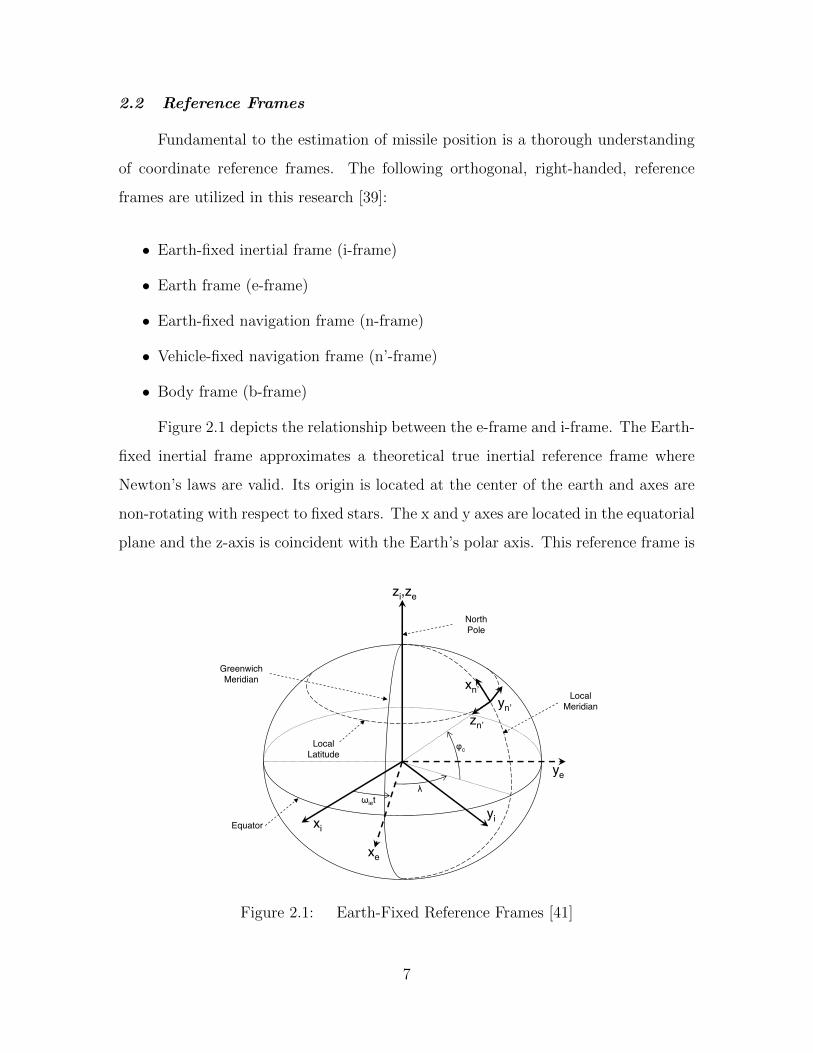
2.2 Reference Frames

Fundamental to the estimation of missile position is a thorough understanding

of coordinate reference frames. The following orthogonal, right-handed, reference

frames are utilized in this research [39]:

• Earth-fixed inertial frame (i-frame)

• Earth frame (e-frame)

• Earth-fixed navigation frame (n-frame)

• Vehicle-fixed navigation frame (n’-frame)

• Body frame (b-frame)

Figure 2.1 depicts the relationship between the e-frame and i-frame. The Earth-

fixed inertial frame approximates a theoretical true inertial reference frame where

Newton’s laws are valid. Its origin is located at the center of the earth and axes are

non-rotating with respect to fixed stars. The x and y axes are located in the equatorial

plane and the z-axis is coincident with the Earth’s polar axis. This reference frame is

xi

xe

ye

yi

zi,ze

xn’yn’

zn’

Greenwich

Meridian

Local

Meridian

!iet

Equator

North

Pole

"

#cLocal

Latitude

Figure 2.1: Inertial, Earth and vehicle-fixed navigation frame.The inertial and Earth frames originate at the Earth’s center ofmass while the vehicle-fixed navigation frame’s origin is locatedat a fixed location on a vehicle.

rotates with respect to the e-frame due to translational motion of the vehicle. The i,

e and n’ -frames are illustrated in Figure 2.1. The n-frame is illustrated in Figure 2.2.

The Earth-fixed navigation frame (n-frame) is an orthonormal basis in !3,

with origin located at a predefined location on the Earth, typically on the surface.

The Earth-fixed navigation frame’s x, y, and z axes point in the north, east, and

down (NED) directions relative to the origin, respectively. As in the previous case,

down is defined as the direction of the gravity vector. In contrast to the navigation

frame, the Earth-fixed navigation frame remains fixed to the surface of the Earth.

While this frame is not useful for very-long distance navigation, it can simplify the

navigation kinematic equations for local navigation routes.

The body frame (b-frame) is an orthonormal basis in !3, rigidly attached to the

vehicle with origin co-located with the navigation frame. The x, y, and z axes point

out the nose, right wing, and bottom of an aircraft, respectively. Strapdown inertial

12

Figure 2.1: Earth-Fixed Reference Frames [41]

7

not truly inertial since the Earth rotates around the sun, but it serves as a sufficient

approximation for terrestrial navigation. The Earth frame differs from the Earth-fixed

inertial frame in that the x and y axes rotate with the Earth.

The Earth-fixed navigation frame, illustrated in Figure 2.2, is a local geographic

reference frame with its origin chosen for convenience at a specific point on Earth. The

x, y, and z-axis point in the north, east, and down (NED) directions, respectively. The

down direction is defined by the direction of the local gravity vector. The east, north,

and up (ENU) navigation frame is a commonly used alternative to NED frame. As

suggested by the name, the x, y, and z-axis point in the east, north, and up directions,

respectively. This research utilizes the NED frame during simulations, but transitions

to the ENU frame for flight test. The vehicle-fixed navigation frame is identical to

the Earth-fixed navigation frame except the origin is chosen at some fixed point on

the vehicle.

xe

ye

ze

xn

yn

zn

Earth-fixed

navigation plane

(perpendicular to local gravity)

NORTH

EA

ST

Figure 2.2: Earth-fixed navigation frame. The Earth-fixed navigation frame is aCartesian reference frame which is perpendicular to the gravity vector at the originand fixed to the Earth.

13

Figure 2.2: Earth-Fixed Navigation Reference Frame [41]

8

xb

yb

zb

xb

Figure 2.3: Aircraft body frame illustration. The aircraftbody frame originates at the aircraft center of gravity.

sensors are fixed to the b-frame, although they may not be located at the origin or

aligned with the axes. The b-frame is shown in Figure 2.3.

The camera frame (c-frame) is an orthonormal basis in !3, rigidly attached to a

camera, with origin at the camera’s optical center. The x and y axes point up and to

the right, respectively, and are parallel to the image plane of the camera. The z axis

points out of the camera perpendicular to the image plane. The c-frame is shown in

Figure 2.4.

The binocular disparity frame (c0-frame) is an orthonormal basis in !3, which is

rigidly attached to the lever arm located between cameras in a binocular configuration,

with origin at a specified point on the lever arm. The x, y, and z axes point forward,

right, and down, respectively. The c0-frame is shown in Figure 2.5.

14

Figure 2.3: Aircraft Body Reference Frame [41]

Figure 2.3 depicts the aircraft body reference frame applied in this research.

The body frame x-axis is out the nose of the aircraft, y-axis is out the right wing,

and z-axis is out of the bottom of the vehicle. Roll, pitch, and yaw describe rotations

about the x, y, and z-axis, respectively. The location of the origin is predetermined

as a fixed point on the vehicle. In aircraft the center of gravity is a commonly used

origin for the body frame.

2.3 Coordinate Transformations

Coordinate transformations provide an expression for the relationship between

a vector in different reference frames. The two coordinate transformations pertinent

to this research are direction cosine matrices (DCM) and euler angles. A DCM is a

3× 3 matrix used to express a vector in a different coordinate frame according to

rb = Cbar

a (2.1)

9

where ra is a vector expressed in some arbitrary reference frame a, rb is the same

vector expressed in frame b and Cba is the DCM from frame a to frame b. The element

in the i -th row and the j -th column of Cba represents the cosine of the angle between

the i -th axis of frame a and j -th axis of frame b [39].

Euler angles provide a method for deriving the DCM to transform from one-

coordinate system to another by performing a series of three rotations about different

axes [39]. Rotations of ψ about the z-axis, θ about the y-axis, and φ about the x-axis

are expressed mathematically by the DCMs

C1 =

cosψ sinψ 0

− sinψ cosψ 0

0 0 1

(2.2)

C2 =

cos θ 0 − sin θ

0 1 0

− sin θ 0 cos θ

(2.3)

C3 =

1 0 0

0 cosφ sinφ

0 − sinφ cosφ

(2.4)

When performing a transformation from a navigation frame to an aircraft body

frame, the angle ψ represents the angle between the nose of the aircraft and north.

Similarly, the angles θ and φ represent the pitch and roll of the aircraft, respectively.

The product of these DCMs yields a transformation from the navigation frame to the

body frame according to

Cbn = C3C2C1 (2.5)

10

Using this DCM, a vector rn defined in the navigation reference frame is trans-

formed into the body frame by

rb = Cbnr

n (2.6)

Deriving a DCM for a transformation in the opposite direction, from body frame to

navigation frame, is easily accomplished by taking the transpose of Cbn (i.e., Cn

b =

(Cbn)T ).

2.4 Kalman Filter

Real-world systems are generally stochastic rather than deterministic because

system models are imperfect, measurements available from sensors contain errors, and

uncontrolled disturbances may exist. Therefore, a KF is a commonly used recursive,

data processing algorithm which provides statistically optimal estimates of the states

of a stochastic system. Implementing a KF requires the development of a system

dynamics model and observation model. The dynamics model is designed to capture

the typical behavior of the system in order to predict the changes in states of interest

between measurement updates. The observation model provides the mathematical

relationship between measurements and system states which is required to improve

state estimates based on sensor data. Utilizing these models, the KF updates the state

estimates by optimally weighting the dynamics and observation models according to

their uncertainties. For example, if the sensor accuracy is poor, the gain in the KF

algorithm adjusts to place more trust in the dynamics model.

Several assumptions are necessary to insure estimates are optimal. First, all

system and measurement noises are accurately described by a Gaussian process. Sec-

ond, noise sources are white, meaning their values are uncorrelated in time. Thirdly,

a conventional KF assumes a linear system model in the general state space form

x(t) = F (t)x(t) +B(t)u(t) +G(t)w(t) (2.7)

11

adequately represents the dynamics of the system. The variable x(t) is a vector of

system states, u(t) is a vector of deterministic inputs, and w(t) is a vector of zero-

mean, white, Gaussian system noise sources. The matrices F (t), B(t), and G(t)

describe how the state vector changes based on the current system states, inputs, and

noise.

Since w(t) is a vector of Gaussian processes, it is completely characterized by

its mean and covariance. The noise covariance or strength, designated by the matrix

Q, is a tuning parameter adjusted to improve demonstrated filter performance. A

higher Q indicates more uncertainty in the dynamics model of the system. Finally,

a conventional KF assumes a linear discrete-time observation model in the general

state space form

zk = Hkxk + vk (2.8)

where z is a vector of measurements, the matrix H relates the measurements to

current states, and v is a vector of zero-mean, white, Gaussian measurement noise

sources. The strength of the measurement noise vector is defined as

E[vkvk] = R (2.9)

whereR is a tuning parameter. TheQ-to-R ratio determines whether the filter places

more faith in the dynamics model or observation model.

Since the KF is a discrete-time estimator, the dynamics model must first be con-

verted from a continuous-time differential equation into an equivalent discrete-time

difference equation. There are several methods available for performing this conver-

sion. This research utilizes the Van Loan method [7]. First, using the parameters

from the dynamics model in Equation (2.7), the matrix

12

M =

−F GWGT

0 F T

∆t (2.10)

is constructed where ∆t is the propagation time step. Next, using software capable

of matrix exponentials, solve for

N = eM =

... φ−1Qd

0 φT

∆t (2.11)

Transposing the lower-right partition of N yields the state transition matrix, φ. Fi-

nally, the discrete-time noise strength, Qd, is obtained from the upper-right partition

of N through some basic linear algebra. Using these results, the equivalent difference

equation for the dynamics model is

xk = φk−1xk−1 +Bk−1uk−1 +wk−1 (2.12)

where the discrete Gaussian, white noise sequence has strength Qdk−1. The determin-

istic input is assumed constant over the propagation interval and therefore uk−1 is

identical to u(t) evaluated at the current time. A first order approximation of Bk−1

is

Bk−1 = F−1(t)(φk−1 − I)B(t) (2.13)

where I is the identity matrix.

All the necessary background is now in place to present the KF recursive al-

gorithm. Since the state vector is a function of deterministic inputs and Gaussian

processes, the state vector is also described by a Gaussian probability density func-

tion (pdf). Therefore, all the information about the state vector is captured by keeping

track of its expected value, x, and covariance, P . Using the discrete-time dynamics

model, the equations for KF time propagations between samples are

13

x−k = φk−1x+k−1 +Bk−1uk−1 (2.14)

P−k = φk−1P+k−1φ

Tk−1 +Qdk−1

(2.15)

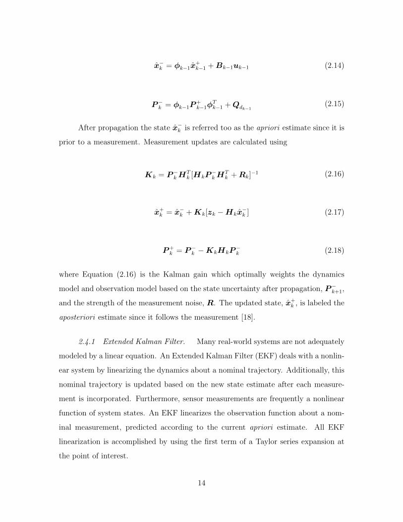
After propagation the state x−k is referred too as the apriori estimate since it is

prior to a measurement. Measurement updates are calculated using

Kk = P−kHTk [HkP

−kH

Tk +Rk]

−1 (2.16)

x+k = x−k +Kk[zk −Hkx

−k ] (2.17)

P+k = P−k −KkHkP

−k (2.18)

where Equation (2.16) is the Kalman gain which optimally weights the dynamics

model and observation model based on the state uncertainty after propagation, P−k+1,

and the strength of the measurement noise, R. The updated state, x+k , is labeled the

aposteriori estimate since it follows the measurement [18].

2.4.1 Extended Kalman Filter. Many real-world systems are not adequately

modeled by a linear equation. An Extended Kalman Filter (EKF) deals with a nonlin-

ear system by linearizing the dynamics about a nominal trajectory. Additionally, this

nominal trajectory is updated based on the new state estimate after each measure-

ment is incorporated. Furthermore, sensor measurements are frequently a nonlinear

function of system states. An EKF linearizes the observation function about a nom-

inal measurement, predicted according to the current apriori estimate. All EKF

linearization is accomplished by using the first term of a Taylor series expansion at

the point of interest.

14

This research is limited to linear missile dynamics models, but applies nonlinear

observation models exclusively. In contrast to Equation (2.8), the general form for a

nonlinear observation model with additive noise is

zk = h[xk] + vk (2.19)

where z is the measurement vector, h[.] is a nonlinear operator, and v is the noise

vector.

In order to linearize this equation about a point of interest, a Jacobian matrix

is calculated by taking the partial derivative of each of the nonlinear functions with

respect to each of the states. Furthermore, the Jacobian is evaluated at the apriori

estimate yielding

Hk =δh

δx|x−

k(2.20)

Next, a nominal measurement is calculated by evaluating the nonlinear function at

the apriori estimate according to

zNk= h[x−k ] (2.21)

Finally, a perturbation state, δz, is defined as the difference between the realized

measurement and nominal measurement

δzk = zk − zNk(2.22)

Since the dynamics model in this research is linear, the conventional KF time

propagation equations are utilized. However, there is one small change in the KF

measurement update equations for the EKF. The aposteriori estimate from Equation

(2.17) is now calculated using

15

x+k = x−k +Kkδzk (2.23)

The rest of the recursive algorithm is unchanged with the exception that the Jacobian

matrix from Equation (2.20) now serves as H in the KF measurement equations.

2.4.2 Unscented Kalman Filter. The Unscented Kalman Filter (UKF) pro-

vides another approach to dealing with nonlinear models. It improves on the accuracy

of the EKF by capturing higher order effects while eliminating the need to calculate

partial derivatives. The EKF is based on applying a first-order Taylor series approx-

imation to linearize a nonlinear function. In contrast, the UKF relies on generating

sigma points to represent the probability density function (pdf) of the state vector.

The nonlinear function for system dynamics is then applied to transform the sigma

points. The new set of sigma points, which represent the transformed pdf of the

state vector, provides the required information to calculate the statistics of mean and

covariance for the apriori estimate. Measurement updates are performed in a similar

manner by transforming the sigma points through the nonlinear observation function

and using the statistics of the sigma points to predict a measurement. The difference

between the realized measurement and the prediction is then used to calculate the

aposteriori estimate. The result is an estimator that accurately represents mean and

covariance of the state vector to third order.

Since only linear dynamics models are utilized in this research, this background

will only cover measurement updates with the UKF. To implement a UKF, sigma

points are carefully chosen to capture the pdf using a fixed number of points based on

the number of states in the system. The number of sigma points required is twice the

number of states plus one. For a measurement update, the sigma points are calculated

from the apriori estimate according to

X0 = x−k (2.24)

16

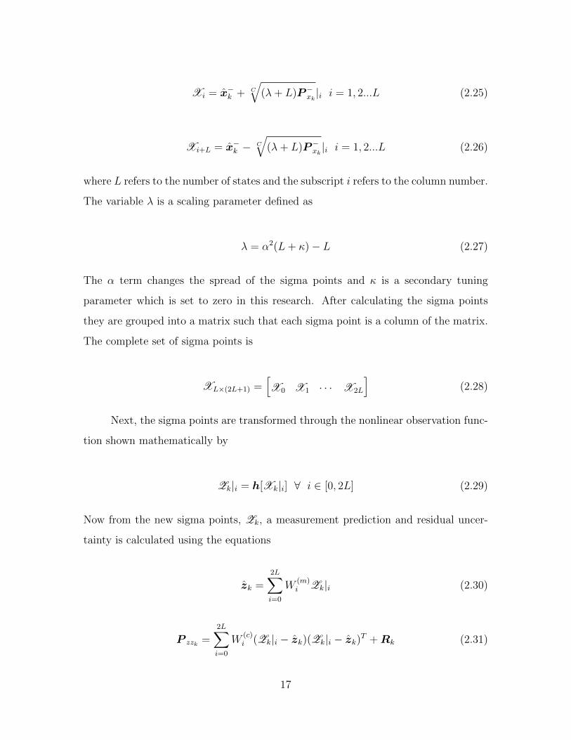
Xi = x−k + C

√(λ+ L)P−xk |i i = 1, 2...L (2.25)

Xi+L = x−k − C

√(λ+ L)P−xk |i i = 1, 2...L (2.26)

where L refers to the number of states and the subscript i refers to the column number.

The variable λ is a scaling parameter defined as

λ = α2(L+ κ)− L (2.27)

The α term changes the spread of the sigma points and κ is a secondary tuning

parameter which is set to zero in this research. After calculating the sigma points

they are grouped into a matrix such that each sigma point is a column of the matrix.

The complete set of sigma points is

XL×(2L+1) =[X0 X1 · · · X2L

](2.28)

Next, the sigma points are transformed through the nonlinear observation func-

tion shown mathematically by

Zk|i = h[Xk|i] ∀ i ∈ [0, 2L] (2.29)

Now from the new sigma points, Zk, a measurement prediction and residual uncer-

tainty is calculated using the equations

zk =2L∑i=0

W(m)i Zk|i (2.30)

P zzk =2L∑i=0

W(c)i (Zk|i − zk)(Zk|i − zk)T +Rk (2.31)

17

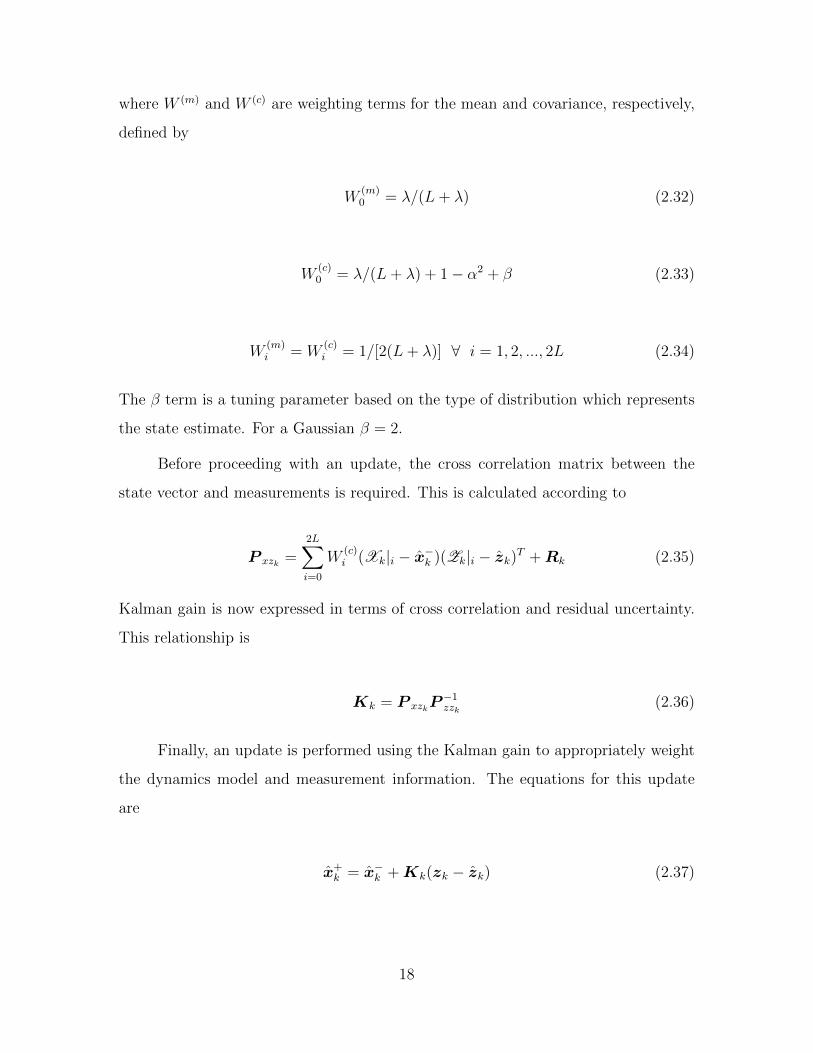
where W (m) and W (c) are weighting terms for the mean and covariance, respectively,

defined by

W(m)0 = λ/(L+ λ) (2.32)

W(c)0 = λ/(L+ λ) + 1− α2 + β (2.33)

W(m)i = W

(c)i = 1/[2(L+ λ)] ∀ i = 1, 2, ..., 2L (2.34)

The β term is a tuning parameter based on the type of distribution which represents

the state estimate. For a Gaussian β = 2.

Before proceeding with an update, the cross correlation matrix between the

state vector and measurements is required. This is calculated according to

P xzk =2L∑i=0

W(c)i (Xk|i − x−k )(Zk|i − zk)T +Rk (2.35)

Kalman gain is now expressed in terms of cross correlation and residual uncertainty.

This relationship is

Kk = P xzkP−1zzk

(2.36)

Finally, an update is performed using the Kalman gain to appropriately weight

the dynamics model and measurement information. The equations for this update

are

x+k = x−k +Kk(zk − zk) (2.37)

18

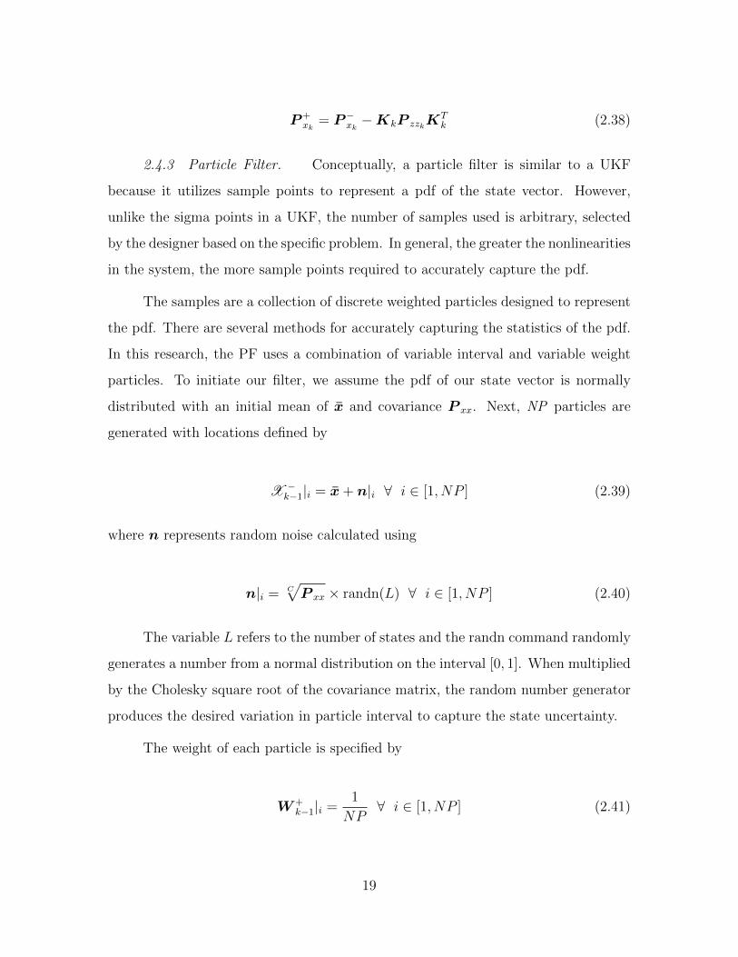
P+xk

= P−xk −KkP zzkKTk (2.38)

2.4.3 Particle Filter. Conceptually, a particle filter is similar to a UKF

because it utilizes sample points to represent a pdf of the state vector. However,

unlike the sigma points in a UKF, the number of samples used is arbitrary, selected

by the designer based on the specific problem. In general, the greater the nonlinearities

in the system, the more sample points required to accurately capture the pdf.

The samples are a collection of discrete weighted particles designed to represent

the pdf. There are several methods for accurately capturing the statistics of the pdf.

In this research, the PF uses a combination of variable interval and variable weight

particles. To initiate our filter, we assume the pdf of our state vector is normally

distributed with an initial mean of x and covariance P xx. Next, NP particles are

generated with locations defined by

X −k−1|i = x+ n|i ∀ i ∈ [1, NP ] (2.39)

where n represents random noise calculated using

n|i = C√P xx × randn(L) ∀ i ∈ [1, NP ] (2.40)

The variable L refers to the number of states and the randn command randomly

generates a number from a normal distribution on the interval [0, 1]. When multiplied

by the Cholesky square root of the covariance matrix, the random number generator

produces the desired variation in particle interval to capture the state uncertainty.

The weight of each particle is specified by

W+k−1|i =

1

NP∀ i ∈ [1, NP ] (2.41)

19

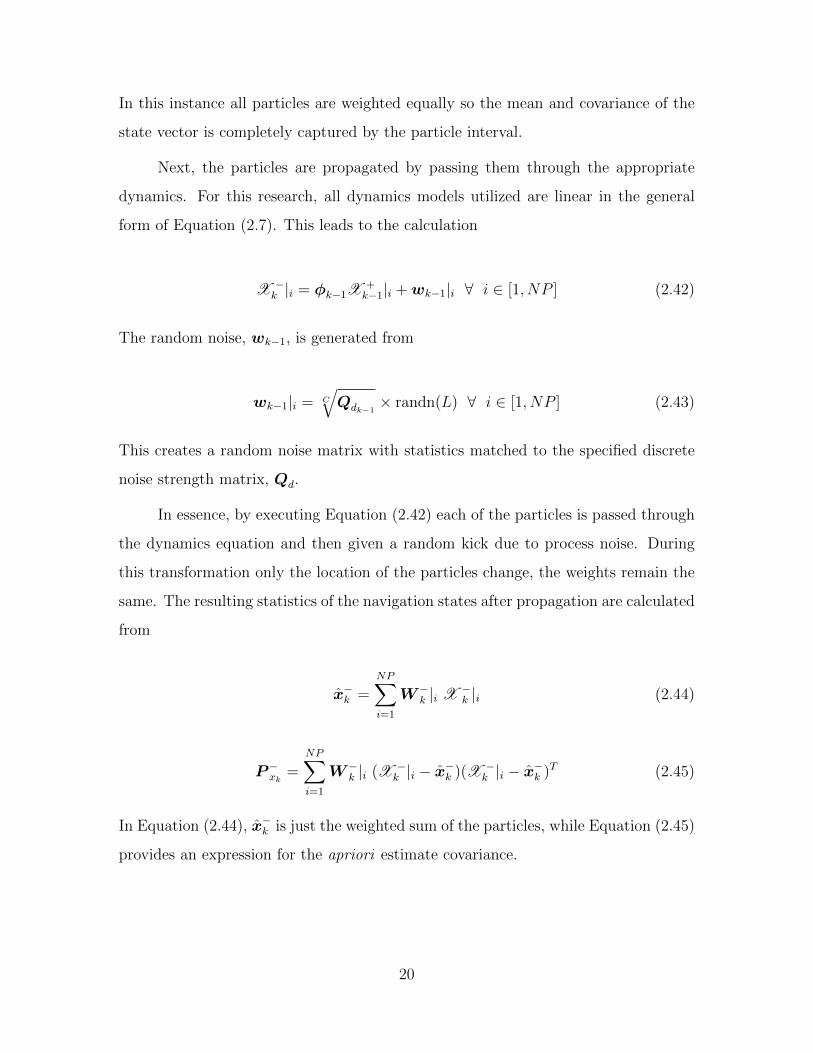
In this instance all particles are weighted equally so the mean and covariance of the

state vector is completely captured by the particle interval.

Next, the particles are propagated by passing them through the appropriate

dynamics. For this research, all dynamics models utilized are linear in the general

form of Equation (2.7). This leads to the calculation

X −k |i = φk−1X

+k−1|i +wk−1|i ∀ i ∈ [1, NP ] (2.42)

The random noise, wk−1, is generated from

wk−1|i = C

√Qdk−1

× randn(L) ∀ i ∈ [1, NP ] (2.43)

This creates a random noise matrix with statistics matched to the specified discrete

noise strength matrix, Qd.

In essence, by executing Equation (2.42) each of the particles is passed through

the dynamics equation and then given a random kick due to process noise. During

this transformation only the location of the particles change, the weights remain the

same. The resulting statistics of the navigation states after propagation are calculated

from

x−k =NP∑i=1

W−k |i X −

k |i (2.44)

P−xk =NP∑i=1

W−k |i (X −

k |i − x−k )(X −k |i − x−k )T (2.45)

In Equation (2.44), x−k is just the weighted sum of the particles, while Equation (2.45)

provides an expression for the apriori estimate covariance.

20

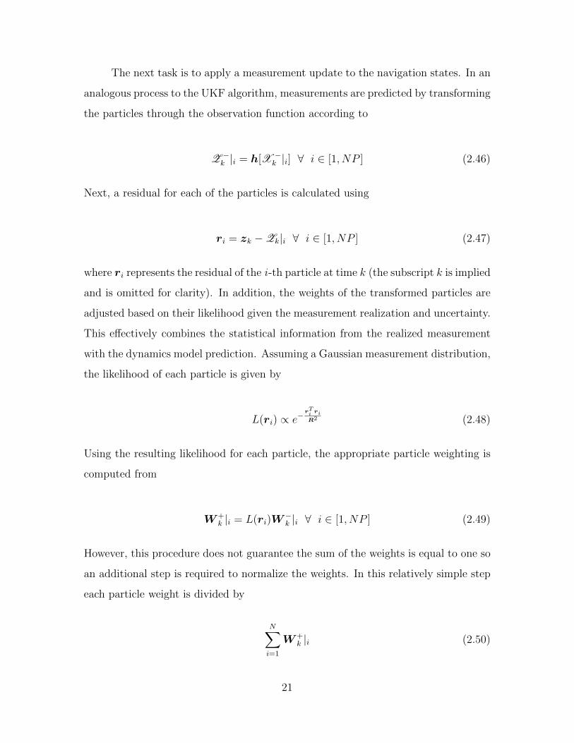
The next task is to apply a measurement update to the navigation states. In an

analogous process to the UKF algorithm, measurements are predicted by transforming

the particles through the observation function according to

Z −k |i = h[X −

k |i] ∀ i ∈ [1, NP ] (2.46)

Next, a residual for each of the particles is calculated using

ri = zk −Zk|i ∀ i ∈ [1, NP ] (2.47)

where ri represents the residual of the i -th particle at time k (the subscript k is implied

and is omitted for clarity). In addition, the weights of the transformed particles are

adjusted based on their likelihood given the measurement realization and uncertainty.

This effectively combines the statistical information from the realized measurement

with the dynamics model prediction. Assuming a Gaussian measurement distribution,

the likelihood of each particle is given by

L(ri) ∝ e−rTi riR2 (2.48)

Using the resulting likelihood for each particle, the appropriate particle weighting is

computed from

W+k |i = L(ri)W

−k |i ∀ i ∈ [1, NP ] (2.49)

However, this procedure does not guarantee the sum of the weights is equal to one so

an additional step is required to normalize the weights. In this relatively simple step

each particle weight is divided by

N∑i=1

W+k |i (2.50)

21

Since the location of the particles does not change during the measurement update

the points are transferred according to

X +k = X −

k (2.51)

This results in a new set of particle locations and weights to use for repeating the

recursive filter algorithm. To calculate an aposteriori state estimate and uncertainty

Equations (2.44) and (2.45) are applied using the post measurement weights and

particle locations.

2.5 Radar Sensor

In this research the observation model is based on a group of sensors providing

range and range-rate information. There are two different categories of radar sensors

capable of providing the desired measurements: pulse-doppler (PD) and frequency-

modulated continuous waveform (FMCW) radar. PD radars are less suitable for short

range applications due to a blind zone in close proximity to the sensors. In addition,

the FMCW sensors are generally lower in cost and complexity making them ideal for

the application in this research.

Continuous wave (CW) radar functions by capitalizing on the Doppler effect.

The CW radar outputs a constant frequency electromagnetic (EM) wave. When the

EM wave reflects off a target and returns to the source, the frequency of the received

signal is shifted based on the relative motion between the source and the target. If the

target has a closing velocity the received frequency is higher while a receding target

results in a lower received frequency. Based on this principle, target velocity along

the sensor line-of-sight is calculated from doppler shift by

v =c(fr − ft)

2ft(2.52)

22

where ft is the transmitted frequency, fr is the received frequency, and c is the speed

of light. In deriving Equation (2.52), it is assumed that c� v.

A FMCW sensor achieves range measurements in addition to range-rate by

systematically varying the frequency of the transmitted signal. Linear frequency

modulation (LFM) is a commonly employed technique in which the transmit frequency

is modulated with a triangular waveform as shown in Figure 2.4 [30].

The bandwidth of the system is described by the frequency sweep range, fsweep.

Furthermore, the chirp time, Tchirp, corresponds to the time required to complete a

sweep from the lowest to highest frequency (labeled TCPI in Figure 2.4). However, this

scheme results in an ambiguous range and range-rate measurement since the receiver

does not know ft for the the received signal at any instant in time. If we plot range

versus velocity on an R-v diagram, the ambiguous combination of range and velocity

describes a line.

In order to resolve the ambiguity, FMCW sensors vary chirp gradients by ad-

justing fsweep and Tchirp. Typical sensors employ four different gradients enabling

an unambiguous measurement of range and velocity by evaluating the intersection of

lines on an R-v diagram as shown in Figure 2.5 [29].

Radar Waveform for Automotive RadarSystems and Applications

Hermann Rohling, Christof MollerInstitute of Telecommunications, Technical University Hamburg-Harburg

Eissendorfer Strasse 40, D-21073 Hamburg, Germanyphone: +49-40-42878-3028, fax: +49-40-42878-2281, email: [email protected]

Figure 1- LFM CW waveform principle

I(t)

The target range R and the radial velocity Vr both cause afrequency shift in the down converted signal denoted as:

(2)

(1)h = 2 fsweep R

c· TCP1

where A is the wavelength of the carrier-frequency. Therange resolution depends in the LFM case directly on thesignal bandwidth !sweep and the resolution in radial velocity vdepends on the observation time TCPl.

II. PURE LINEAR FREQUENCY MODULATION CW PRINCIPLE

The LFM transmit signal is a classical and well knownwaveform [7] for many different radar applications. In thiscase the oscillator sweep and the system bandwidth isdescribed by !Sweep, the chirp duration is called a coherentprocessing interval (CPI) and is described by TCPl.

In this paper three different radar waveforms are consideredfor a more general system requirement, to measure targetrange, radial velocity and azimuth angle simultaneously andunambiguously. The paper is focused on CW based radarsystems due to some important advantages in shortmeasurement time and low computation complexity comparedwith classical pulse radars. It is characteristic for allautomotive radar applications that almost always multipletargets will be observed. Therefore, the target resolutionproperties of the different waveforms play an important role inthe system analysis.

Index Terms- Radar Waveforms, Automotive Radar, CW,FMCW, FSK, Monopulse Technique

I. INTRODUCTION

High performance automotive radar systems are currentlyunder development for various applications. Comfort systemslike Adaptive Cruise Control (ACC) are already available onthe market as 24 GHz and 77 GHz radar sensors. Target range,azimuth angle and radial velocity are measured in this casesimultaneously with high resolution and accuracy even inmulti target situations. Future radar sensor developments willbe more concentrated on safety applications like CollisionAvoidance (CA), Pre Crash (PC) or even Autonomous Driving(AD). In this case the system requirements for target detectionreliability (extreme low false alarm rate), measurementaccuracy and reaction time (extreme short measurement time)will be much stronger and much more important comparedwith today ACC systems.

To meet all these system requirements in automotiveapplications, very specific waveform design techniques shouldbe considered. For ACC systems both radar types of aclassical pulse waveform with ultra short pulse lengths (30 ns)or alternatively continuous wave (CW) and LFM waveformwith a bandwidth of 150 MHz (and a resulting rangeresolution of 1m) have been proposed and developed.

Abstract-This paper describes three different continuouswave (CW) radar waveforms which are applied in automotiveradar sensors. The radar sensor should be able to detect allobjects inside the observation area and to estimate range, radialvelocity and azimuth angle simultaneously even in multi targetsituations.

A classical Linear Frequency Modulation (LFM) waveformprovides a very high range and velocity resolution. But inmultiple target situations so-called ghost targets will occur.Alternatively, a Frequency Shift Keying (FSK) waveform deliversa very high velocity resolution and avoids any ghost targetsituation but will not resolve targets in range direction. Finally, acombination between LFM and FSK provides simultaneously ahigh range and velocity resolution, extremely short measurementtime and avoids any ghost target situation. It combines theadvantages of both FSK and LFM waveforms. In all three casesthe azimuth angle estimation is based on two receive antennasand the monopulse technique.

1-4244-1 539-X/08/$25.00 ©2008 IEEE

Authorized licensed use limited to: Air Force Institute of Technology. Downloaded on April 19,2010 at 19:40:39 UTC from IEEE Xplore. Restrictions apply.

Figure 2.4: Linear Frequency Modulation in an FMCW Radar Sensor

23

!"#"$%"!& '("& "#()& *$+,-.& $*& /)0,& #),%"!'"/& 12& '("

$,*'-,'-,")3*&4!"53",#2&$,')&1-*"&1-,/&-,/&*-67."/&! &'$6"*8

9("& 4!"53",#2& *'"7& "#$%&' ((( −= & $*& *6-..& -,/& 0$..& 1"

#()*",& $,& /"7",/",#"& )4& '("& 6-:$636& 3,-61$+3)3*& '-!+"'

!-,+"8&9("&'$6";/$*#!"'"&!"#"$%"&*$+,-.&$*&<)3!$"!&'!-,*4)!6"/

$,&"-#(&=>?&)4& .",+'(& )*+, &-,/& '-!+"'*&0$..&1"&/"'"#'"/&12

-,& -67.$'3/"& '(!"*()./& @=<ABC8& D3"& ')& '("& *6-..& 4!"53",#2

*'"7&$,&'("&'!-,*6$'&*$+,-.&-&*$,+."&'-!+"'&0$..&1"&/"'"#'"/&-'&'("

*-6"& D)77."!& 4!"53",#2& 7)*$'$),& $,& '("& -/E-#",'& =>?F*& 13'

0$'(& /$44"!",'& 7(-*"& $,4)!6-'$),& ),& '("& '0)& *7"#'!-.& 7"-G*8

9("&7(-*"&/$44"!",#"& "# ϕϕϕ −=∆ & $,& '("&#)67.":&*7"#'!-

$*& '("& 1-*$*& 4)!& '("& '-!+"'& !-,+"& - & "*'$6-'$),8& 9("& !".-'$),1"'0"",& '("& '-!+"'& /$*'-,#"& -,/& 7(-*"& /$44"!",#"& $*& +$%",& 12

'("&4)..)0$,+&"53-'$),

$%&'(

.-

⋅∆⋅−=

πϕ

H8 @IC

9)& -#($"%"& -,& 3,-61$+3)3*&6-:$636& !-,+"&6"-*3!"6",'

)4&IJK&6&-&4!"53",#2&*'"7&)4& LMN&I=$%&'( &$*&,"#"**-!28&?,

'($*&#-*"&'("&'-!+"'&!"*).3'$),&),.2&/"7",/*&),&'("&=>?&.",+'(

)*+, 8& 9("& '"#(,$#-..2& *$67."& O=P& 6)/3.-'$),& $*& -,

-//$'$),-.& -/%-,'-+"& )4& '($*& 0-%"4)!68& Q3'& '($*& <RS

0-%"4)!6& /)"*& ,)'& -..)0& -,2& '-!+"'& !"*).3'$),& $,& '("& !-,+"

/$!"#'$),T& 0($#(& $*& -,& $67)!'-,'& /$*-/%-,'-+"& )4& '($*

6"-*3!"6",'& '"#(,$53"8& U*7"#$-..2& $,& -3')6)'$%"& '!-44$#

",%$!),6",'& 6)!"& '(-,& -& *$,+."& 4$:"/& '-!+"'& 0$..& )##3!

*$63.'-,")3*.2& $,*$/"& -,& -,'",,-& 1"-68& 9("*"& 4$:"/& '-!+"'*

#-,&,)'&1"&!"*).%"/&12&-&<RS&0-%"4)!68

???8! >VBU&W?XUAB&<BUYVUX=Z&LPDVWA9?PX

>B?X=?>WU

B-/-!*& 0($#(& -77.2& 73!"& .$,"-!& 4!"53",#2& 6)/3.-'$),

'"#(,$53"& @W<LC& 6)/3.-'"& '("& '!-,*6$'& & 4!"53",#2& 0$'(& -

'!$-,+3.-!& 0-%"4)!6& [R9P\]^8& 9("& )*#$..-')!& *0""7& $*& +$%",

12& $/&&'( 8& A& '27$#-.& %-.3"& 4)!& '("& 1-,/0$/'(& $*

LMN&IJK=$/&&'( & ')& -#($"%"& -& !-,+"& !"*).3'$),& )4

6&I]

=⋅

=∆$/&&'(

.- 8& ?,& +","!-.T& -& *$,+."& *0""7& )4& '("

W<L&0-%"4)!6&+$%"*&-,& -61$+3)3*&6"-*3!"6",'& $,& !-,+"&-

-,/& !".-'$%"&%".)#$'2&08&9("&/)0,&#),%"!'"/& !"#"$%"& *$+,-.& $*

*-67."/& -,/& <)3!$"!& '!-,*4)!6"/& $,*$/"& -& *$,+."& =>?8& ?4& -

*7"#'!-.&7"-G& $*&/"'"#'"/& $,& '("&<)3!$"!& *7"#'!36&-'& $,/":&κ@,)!6-.$N"/&$,'"+"!&4!"53",#2C&'("&-61$+3$'$"*&$,&'-!+"'&!-,+"

-,/& %".)#$'2& #-,& 1"& /"*#!$1"/& $,& -& - ;0 ;/$-+!-6& 12& '("4)..)0$,+&"53-'$),

κκ +∆

=∆

⇔∆

−∆

=-

-

0

0

-

-

0

0T @]C

0("!"& 0∆ &/"*#!$1"*&'("&%".)#$'2&!"*).3'$),&!"*3.'$,+&4!)6&'("

=>?& /3!-'$),& )123', @ 6_*&8K]

=⋅

=∆)123',

0λ

T& λ & $*& '("

0-%".",+'(&)4&H&66&a&bb&cMN&-,/& 6*&J8]=)123', C8

& ν

-

,435&%676

,435&%686

9&%&.%&96'&4:;6(<3

<$+8&]8&d&":-67."&-=0=/$-+!-6&4)!&'0)&'-!+"'*&6"-*3!"/&0$'(&37&#($!78

<$+8&]&*()0*&-,&":-67."&$,*$/"&'("&-;0 ;/$-+!-6&4)!&-&'0)'-!+"'&*$'3-'$),&6"-*3!"/&0$'(&-&*$,+."&#($!78&U-#(&.$,"&/!-0,

$,&<$+8&]&#)!!"*7),/*&')&-&6"-*3!"/&*7"#'!-.&.$,"&-'&$,/":&&κ$,/$#-'$,+& -..& *).3'$),*& 4)!& "53-'$),& ]& -,/& -..& 7)**$1."

#)61$,-'$),*&)4&'-!+"'&B-,+"&-&-,/&%".)#$'2&8

<)!& !"-*),& )4& !"*3.'$,+& !-,+";%".)#$'2& -61$+3$'$"*& 43!'("!

6"-*3!"6",'*&0$'(& /$44"!",'& #($!7& +!-/$",'*& $,& '("&0-%"4)!6

-!"& ,"#"**-!2& ')& -#($"%"& -,& 3,-61$+3)3*& !-,+";%".)#$'2

6"-*3!"6",'& "%",& $,&63.'$;'-!+"'& *$'3-'$),*8&9("&0"..& G,)0,

37;_& /)0,;#($!7& 7!$,#$7."& -*& $'& $*& /"7$#'"/& $,& <$+8& I&@1C& $*

/"*#!$1"/&$,&/"'-$.&$,&[e^8&W<L&0-%"4)!6*&#-,&1"&3*"/&"%",&$,

63.'$;'-!+"'&",%$!),6",'*T&13'&'("&":'",/"/&6"-*3!"6",'&'$6"

$*&-,&$67)!'-,'&/!-01-#G&)4&'($*&W<L&'"#(,$53"8

&

'

4@'C

-

0

9#($!7

@-C& @1C

<$+8&f8&d&@-C&0-%"4)!6&4)!&3*"&$,&63.'$&'-!+"'&*$'3-'$),*&-,/&@1C&#)!!"*7),/$,+

":-67."&-;06;/$-+!-6&4)!& &-& '0)&'-!+"'&*$'3-'$),&-,/&'("&!".-'"/&$,'"!*"#'$),

7)$,'*

?,&63.'$&'-!+"'&*$'3-'$),*&-&0-%"4)!6&-*&*()0,&$,&<$+8&f&@-C

$*&3*"/&0($#(&#),*$*'*&)4&H&/$44"!",'&#($!7&*$+,-.*8&?,&+","!-.T

'("& 4!"53",#$"*&6)/3.-'$),&0$..& 1"& /$44"!",'& $,& "-#(& )4& '("& H

#($!7*8&?,&"-#(&#($!7&*$+,-.&-..& '-!+"'*&-!"&/"'"#'"/&0($#(&*'$..

43.4$.&"53-'$),&@]C8&9("&/"'"#'"/&*7"#'!-.&.$,"*&4!)6&-..&H&#($!7

*$+,-.*& #-,& 1"& /!-0,& $,& -& *$,+."& -;0 ;/$-+!-6& @<$+& f& @1CC0("!"& '("&+!-/$",'& )4& -& *$,+."& .$,"& $*& /"7",/",'& ),& '("& #($!7

*0""7& !-'"8& ?,& 63.'$7."& '-!+"'& *$'3-'$),*& 6-,2& $,'"!*"#'$),*

1"'0"",& .$,"*& )4& /$44"!",'& -,/& -/E-#",'& #($!7*& -77"-!& -*& '("

":-67."& $,& <$+& f& @1C& *()0*8& ?4& *3#(& -,& $,'"!*"#'$),& 7)$,'

)##3!*& 0($#(& (-*& ,)& 7(2*$#-.& !"7!"*",'-'$),& )4& -& !"4."#'$),

)1E"#'&$'&$*&#-.."/&-&+()*'&'-!+"'8&A&!"-.&'-!+"'&$*&!"7!"*",'"/&12

-,&$,'"!*"#'$),&7)$,'&1"'0"",&-..&#),*$/"!"/&&H&.$,"*8

Figure 2.5: FMCW Sensor Employing Varying Chirp Gradient to Resolve Range-Velocity Ambiguity

The range and velocity resolution for an FMCW sensor are calculated by

∆R =c

2fsweep(2.53)

∆v =λ

2Tchirp(2.54)

2.6 Multilateration

Estimating missile position based on sensor range measurements relies on the

concept of trilateration. Figure 2.6 demonstrates a simple 2D case of trilateration

where three sensors, P1, P2, and P3, measure range to a target located at point B.

Given a single range measurement from sensor P1, the 2D position of the target is

constrained to lie somewhere along the circle of radius r1 around the sensor. If a

second sensor, P2, simultaneously provides a range measurement of r2, the target

position must be at an intersection of the two circles. As depicted in Figure 2.6, the

intersection of the two circles limits the possible target location to two points, A and

B. Finally, range from a third sensor, P3, uniquely identifies the 2D target location

as point B. An inherent limitation in applying this approach is the sensors cannot be

co-linear. For example, if we move the location of sensor P3 such that all sensors lie

along a single straight line, their circles would all intersect at points A and B. In this

case sensor P3 does not provide any additional information and the 2D position of

24

Figure 2.6: 2D Trilateration [14]

the target is not uniquely determined except in the trivial case in which the target is

also co-linear with the sensors.

In 3D space, four non-coplanar sensors are required to uniquely define target

location. The range from a single sensor describes a sphere around the object. Adding

a second sensor constrains target position to the intersection of two spheres (i.e., a

circle). Finally, by adding a third and fourth sensor range, the 3D position is further

limited to a single point as discussed in the 2D example. In many applications three

sensors are actually sufficient for updating 3D position because one of the two poten-

tial locations can be eliminated based on feasibility. As an example, GPS receivers

determine user position by measuring ranges from multiple satellites. Although a

minimum of four satellites are required to solve for receiver position, one of these

satellites is actually necessary to determine an unknown clock bias to insure satellite

ranges are accurate [24]. The remaining three satellites are sufficient to uniquely solve

25

for the user’s location because only one of the two possible receiver locations is on

the surface of the Earth [24]. The remaining point is somewhere in distant space and

can be disregarded.

If all of the available range measurements are perfect, utilizing more than three

sensors will not change the target location because all sensors’ ranges will intercept

at exactly the same point. However, in reality every sensor range measurement is

corrupted by random noise. As a result, position accuracy is improvable by using

range measurements from more than three sensors, referred to as multilateration [24].

This process assumes each sensor measurement is unbiased and applies a least-squares

error estimation to calculate the target location [24].

When calculating position based on imperfect measurements sensor geometry

is critical. Figure 2.7 illustrates the increase in error which results from suboptimal

geometry. In Figure 7(a) the estimated target location is point A based on range

measurements from sensors one and two. These sensors are configured such that their

angular spacing from the target viewpoint is 90 degrees. The solid circles indicate

the measured range between the target and each sensor while the dashed line repre-

sents measurement uncertainty (i.e., the true range from each sensor is expected to

fall somewhere between their respective dashed circles). Based on this geometry, the

1

2

A

(a) Optimal Geometry

1

2

A

(b) Poor Geometry

Figure 2.7: Impact of Sensor Geometry on Precision of Position Calculation [24]

26

gray shaded region indicates the region of uncertainty for the target location. Fig-

ure 7(a) represents the optimal geometry because area of uncertainty is minimized

(i.e., the precision of the location estimate is maximized). In contrast, Figure 7(b)

demonstrates the reduction in precision resulting when the sensor geometry is less

than optimal. In a two sensor case, a 90 degree angular separation is desired between

the sensors. However, for more than two sensors the best geometry is achieved when

the angular spacing, θ, is

θ =360

N

◦, N > 2 (2.55)

where N is the number of sensors. For example, if you have three sensors the optimal

configuration is an angular separation of 120◦ as viewed from the target. The concept

is easily extended to 3D location precision.

2.7 Velocity Vector Calculation from Speed Measurements

A target’s velocity vector is calculated by utilizing radial velocity measurements

from multiple sensors in a process similar to multilateration. Figure 2.8 depicts a

S1 S2

T

V1

V2

V

!

Figure 2.8: Calculation of 2D Velocity from Speed Measurments [26]

27

simple 2D scenario for illustration. In this example, two sensors, S1 and S2, perform

speed measurements of the target, T , along their LOS to the target. Assuming target

and sensor positions are known, the velocity vector of the target is estimated by the

projections v1 and v2 as depicted in Figure 2.8. By examining the geometry in the

figure, it is apparent that a minimum of two sensors are required for a 2D velocity

vector and the sensors cannot be positioned along the same LOS from the target (i.e.,

both sensors and the target cannot lie along a straight line). This process is extended

to 3D by increasing the sensor count to three and insuring that all sensors are not

co-planar with the target and no two sensors are co-linear with the target.

All of the geometry considerations relevant to multilateration also apply to

precise velocity vector calculation. For example, in the 2D case depicted in Figure 2.8,

the ideal geometry occurs when θ = 90◦. The error in the calculated velocity vector

increases as the angle decreases towards zero degrees [35].

2.8 Gating and Data Association

Tracking a target in a cluttered environment requires a method for eliminating

false observations while associating valid observations with an existing target. Gating

and data association techniques address this issue.

Gating approaches the task of distinguishing true target observations from clut-

ter by evaluating the distance between the expected measurement and each received

measurement. Two types of gating, square and ellipsoidal, are relevant to this re-

search. Square gating is applied as a computationally cheap method to quickly elimi-

nate observations far from the expected track location. To perform square gating the

maximum eigenvalue of the residual covariance scaled by the selected gate size, γ, is

evaluated according to [5]

emax =√

max(eig(γS)) (2.56)

28

The gate size is selected to achieve a desired probability that a true observation will fall

within the selected gate. For example, choosing γ = 9.2 provides a 99 percent chance

that the true observation is within the gate [5]. The residual covariance is calculated

from the apriori state covariance, P−k , and the measurement model parameters using

the formula [5]

Sk = HkP−kH

Tk +Rk (2.57)

After computing emax, each measurement, zj, is compared to the expected

target measurement, z, using the formula [5]

z − emax ≤ zj ≤ z + emax (2.58)

The subscript j refers to the j -th measurement from the sensor. Every measurement

outside this region is eliminated as a possible candidate for updating the target.

If multi-target tracking is employed, these unused measurements are evaluated for

updating alternate targets or initiating new targets.

Square gating only provides a coarse evaluation of potential observations because

it’s based on the residual covariance in the worst case direction of the measurement

space. Ellipsoidal gating is used to further reduce observations relevant to the target

by comparing the residual norm of each measurement to the gate size. The residual

norm, d2j , is calculated by [12]

d2j = δzTj S

−1δzj (2.59)

where the time subscript, k, is intentionally omitted for clarity. If d2j > γ, the

observation is eliminated as an option for target update [12]. If multiple observations

lie within the target’s ellipsoidal gate, data association is applied to select the most

likely candidate for target update.

29

There are two broad categories for data association, hard assignments and soft

assignments. In a hard assignment a maximum of one observation is associated with

each target. This is computationally simple, but performance is generally only satis-

factory for basic tracking scenarios. In comparison, soft assignments allow association

of multiple observations with a single target. This method is accomplished by prob-

abilistic weighting of the measurements within the track’s gate.

Although numerous different options are available for data association, this

research applies the simplest technique, the global nearest neighbor (GNN). This

hard assignment approach works well for our application involving a single-target in a

low clutter environment. Based on GNN, the closest observation within each track’s

ellipsoidal gate is selected to perform the update. The closest observation is assessed

by comparing the residual norm, d2j , for each observation surviving gating. [12]

2.9 Past Research

Missile state parameter estimation is a topic addressed by researchers in a va-

riety of different applications. Some literature specifically addresses the problem of

performing air-to-air missile scoring using various approaches such as radar, GPS,

infrared or lasers. Other relevant literature applies similar concepts to the problem of

tracking a ballistic missile trajectory for predicting impact location and performing

an intercept. Although there are significant differences between these problems, there

are also substantial similarities in approaches to solving the problems. For example,

researchers commonly employ missile modeling in conjunction with Kalman filtering

algorithms to estimate missile state parameters. Section 2.9.1 will summarize some

of the research related to missile state parameter estimation to include scoring sys-

tems for test and evaluation, countermeasures systems for defeating air-to-air missiles,

ballistic missile tracking approaches, and complex missile dynamics models.

Section 2.9.2 explores research with related methodologies, but not directly

associated with missile state parameter estimation. Although the applications are

30

different, this research illustrates examples of utilizing multilateration, range-rate

measurements, and Kalman filtering to estimate the position or velocity of a target.

2.9.1 Missile Tracking. DiFillippo and Campbell [8] present a concept for an

active missile approach warning system (MAWS) similar to the end-game vector scor-

ing system proposed in this research. The proposed MAWS utilizes a pulsed Doppler

radar on the target platform to detect incoming missiles and direct the employment

of countermeasures. The radar provides range and range-rate information to an EKF

software algorithm to perform estimation of the missile parameters. DiFillippo and

Campbell utilize a complex nonlinear missile dynamics model in the general form

x(t) = f(x, t) +w(t) (2.60)

This research expands on their work by considering additional missile dynamics mod-

els and evaluating alternate nonlinear Kalman filters such as the UKF and PF. Ad-

ditionally, this research evaluates estimation performance using COTS, automotive-

grade radar sensors. Furthermore, the authors mention the application of gating, but

do not discuss specific implementation.

In 1997, Bradley received a patent on his invention of a miss distance vector

scoring system [6]. The invention provides miss distance and miss direction in azimuth

and elevation from the target. This device utilizes four omni-directional antennas

emitting RF energy in a spherical pattern. Reflected energy is received by each of

the four antennas and processed to provide direction and distance of the missile.

This simple hardware only setup does not incorporate Kalman filtering or similar

estimation techniques, nor does it model missile dynamics.

Minor and Rowe suggest a different approach to missile scoring using an inte-

grated GPS receiver and micro-electro-mechnamical system (MEMS) as an inertial

sensor embedded in the missile or rocket [22]. Although there are advantages to this

approach, there are also several disadvantages as outlined in Chapter I. Stadnik’s

31

research, presented in [33], demonstrates the feasibility of implementing a GPS trans-

lator onto a missile system. However, a GPS based scoring system could incorporate

the Kalman filter algorithms and missile dynamics models presented in this research

to improve missile state estimation.

There is a significant body of literature exploring methods for passively tracking

targets with IR sensors. Passive IR sensors do not offer an inherent advantage in test

and evaluation applications, but do offer significant benefits for MAWS since they

do not increase risk of detection. Dikic and Kovacevic [13] present a solution for air

targets with two IR detectors. The IR sensors provide angle-only measurements to a

filter based on interacting multiple models (IMM). An IMM algorithm uses a bank of

Kalman filters, each with a different missile dynamics model. During target estima-

tion, the algorithm can jump between the subfilters based on observed measurements

to improve missile state estimation performance. This setup offers advantages when

tracking a missile over an extended period of time involving multiple different phases

of flight. For example, an air-to-air missile tracked from launch, through boost, coast,

and endgame maneuvering would presumably demonstrate significantly different mo-

tion and a single dynamics model will not accurately capture all these phases. For

end-game missile scoring, an IMM algorithm is unlikely to show significant perfor-

mance improvement. The problem addressed by Dikic and Kovacevic is limited to

estimating the scalar range from missile to target rather than a 3D vector solution.

In related research, Xu, Wang, Zhao, and Guo propose a method for extracting range

from a single IR sensor based on image processing [42].

The concept of single or combinations of IR sensors producing range information

provides exciting implications for aircraft defensive systems. The air-to-air missile

scoring system proposed in this research could be adapted to a MAWS system by

substituting passive IR sensors for the FMCW sensors. However, performance will

depend on the accuracy of the range measurements provided by the IR sensors.

32

A brief examination of research regarding ballistic missile tracking is also useful

for considering approaches to missile vector scoring. Siouris, Chen, and Wang propose

the tracking of an incoming ballistic missile using an extended interval Kalman filter

(EIKF) [31]. Like many ballistic missile tracking approaches, the authors assume the

availability of range, azimuth, and elevation measurements from a ground based radar

system. Using this as the basis for their observation model combined with a nonlinear

dynamics model, an EIKF algorithm is implemented. The EIKF was designed for

nonlinear systems with parameter uncertainties that can be described by intervals.

Conceptually, this is similar to the concept of switching between different dynamics

models to model a missile during different phases of flight. There is a substantial

amount of additional research available on different approaches to tracking a ballistic

missile in which different dynamics models and filtering methods are explored. Much

of the research is summed in Minvielle’s article in [23]. The interested reader is also

referred to [9] for a discussion of tracking ballistic missiles using IMM.

Any attempt to estimate missile state kinematic parameters using Kalman filter-

ing must consider the appropriate missile dynamics model to obtain desired accuracy.

Blackman and Popoli [5] outline several different missile models including constant ve-

locity (CV), constant acceleration (CA), a three-dimensional coordinated turn (CT),

and first-order Gauss-Markov acceleration (FOGMA). Several authors [28] [37] sug-

gest hybrids of the CV and CA models by incorporating real-time switching between

the dynamics models to improve tracking performance. More advanced missile models

are proposed through research by other authors. Maybeck, Negro, Cusumano, and

De Ponte develop a refined missile acceleration model by exploiting a knowledge of

aerodynamically induced lift and drag forces of a nonthrusting missile employing pro-

portional navigation guidance [17]. Their nonlinear missile dynamics model assumes

additive, zero-mean, white, Gaussian noise. In addition, they utilize an observation

model in which noise corrupted measurements of range, range-rate, and LOS angle

are available. An EKF based on these models is proposed to assist in the precise

tracking and prediction of the parameters of a threat missile.

33

The end-game air-to-air missile scoring system proposed in this paper inten-

tionally does not utilize LOS angle measurements. This setup would require a more

complex and expensive tracking radar which may be impractical for test and evalu-

ation where drone aircraft destruction is anticipated. Additionally, the setup would

require multiple tracking radars due to field of view (FOV) limitations and aircraft

masking issues. Several of the dynamics models mentioned above are considered in

this research, however, simpler linear models are selected over more complex nonlin-

ear models like the one proposed in [17]. In missile testing, all the data processing is

performed post-mission and highly accurate dynamics models for predictive purposes

are unnecessary.

2.9.2 Related Estimation Problems. In the past, researchers applied tri-

lateration in conjunction with Kalman filtering to a number of different navigation

problems with highly successful results. Miah and Gueaieb use this approach for 2-

dimensional (2D) navigation of a robot in [21]. In their work, a robot is equipped

with a radio frequency identification (RFID) reader and three RFID tags are placed

at known 3D locations in an indoor environment. This setup provides distance mea-

surements between the robot and three known locations. Since the RFID tags are

arranged in 3D space, three ranges does not uniquely identify the location of the

robot, but the author uses a geometric approach based on Cayley-Menger determi-

nants to solve the localization problem. Next, the author develops a dynamics model

for the robot motion which includes zero-mean, white, Gaussian system noise. The

dynamics model and observation model are implemented in an EKF and UKF to

better estimate the robot position during navigation. Since this is a 2D navigation

problem, the states of interest are the x and y position of the robot. The author

concludes by performing an indoor navigation simulation and comparing the position

estimates of the robot provided by trilateration alone, and trilateration in conjunction

with the two proposed Kalman filters. The results are summarized in Figure 2.9. As

illustrated in this figure, incorporating Kalman filtering reduces the root mean square

34

(a) Root Mean Square Error for Open Loop RobotPath

(b) Root Mean Square Error for Closed LoopRobot Path

Figure 2.9: Comparison of Errors using Three Different Estimation Techniques for2D Robot Navigation [21]

error (RMSE) significantly. The average RMSE for the UKF estimates are reduced

by a factor of approximately 6.

This research paper proposes a similar method for performing air-to-air missile

vector scoring. A multiateration observation model is incorporated into an EKF

and UKF to improve missile state estimation. However, the missile state estimation

problem is significantly more complex for a variety of reasons. First, the missile

estimation problem is 3D and test and evaluation applications are interested in missile

velocity as well as position. Additionally, modeling missile dynamics accurately is

more challenging than capturing robot dynamics. The majority of the robot motion

is controlled by deterministic inputs and hence, easy to model. However, the research

by Miah and Gueaieb provides some useful insights by demonstrating the potential for

significant improvement in state estimation by incorporating Kalman filtering rather

than using trilateration stand-alone.

Tu and Kiang [40] propose a different strategy for applying trilateration and

Kalman filtering to estimate the position, velocity and acceleration of a vehicle to

avoid collision. The approach assumes a vehicle equipped with a minimum of three

sensors providing range, radial velocity, and radial acceleration using hybrid linear

frequency modulation (LFM)/frequency shift keying (FSK) echoed signals. Measure-

ments from each sensor to a target vehicle are separately processed through a linear

Kalman filter and then combined through the trilateration process to determine 2D

35

position, velocity, and acceleration of the target as illustrated in Figure 2.10. The au-

thors demonstrate the effectiveness of this approach, referred to as a robust Kalman

filter (RKF), in several scenarios. In related work, Klotz uses a network of FMCW

sensors to trilaterate a target for vehicle collision avoidance [15]. He presents a solu-

tion using a least squares estimate of an overdetermined solution without a Kalman

filter and an additional approach incorporating an EKF. Tu and Kiang compare their

RKF solution to an EKF based approach and conclude the RKF performs better

when the target vehicle is turning over a short period of time.

The method proposed in the next chapter for air-to-air missile vector scoring

considers EKF, UKF, and PF based approaches in lieu of a RKF, but an RKF is an

option for future work. Although the approaches cited in the collision avoidance auto-

motive research are relevant to the proposed missile scoring system, they are simpler

problems like robot navigation. Automotive collision avoidance is a 2D problem and

the velocity and acceleration of the target vehicles does not approach the expected

values for a missile.

The medical field contains research examples related to the relevant concept of

converting multiple range-rate measurements into velocity. Torricelli, Scabia, Biagi,

and Masotti [27] suggest a 2D vector Doppler system for use in observing patient

Figure 2.10: Procedure for a Robust Kalman Filter [40]

36

blood flow. Steel and Fish contribute to this field by studying the impact of range-

rate measurement errors on the resulting estimated 2D or 3D velocity vectors [34].

These works are not based on Kalman filtering, but they provide insights into strate-

gies for locating range-rate sensors and anticipating velocity error magnitude. The

mathematical background for velocity calculations in Section 2.7 is taken directly

from these conference papers.

2.10 Summary

This chapter began by covering the mathematical background required to un-

derstand the methods presented in the next chapter. The mathematical notation

applied throughout this research was covered in great detail. The relevant coordinate

reference frames were described along with transformations used to transition between

reference frames. Additionally, the Kalman filter recursive data processing algorithm

was presented along with an explanation of the three specific nonlinear Kalman filters

applied in this research: an EKF, UKF, and PF. Furthermore, the basic operation

of FMCW radar was described to familiarize the reader with the sensors used in

the proposed missile scoring system. Moreover, the mathematical concepts required

to determine target 3D position and velocity using multiple sensor measurements of

range and range-rate were presented. Finally, this chapter introduced gating and data

association to reduce the impact of radar clutter on missile state estimation.

The chapter concluded with a brief review of prior research to illustrate the

contributions of this research with an academic framework. The past research was

divided into two areas, work directly related to missile tracking and work employing

similar methods for different types of estimation problems. In the next chapter,

the methodology for implementing the proposed air-to-air missile scoring system is

presented.

37

III. Methodology

This research proposes an end-game missile scoring system which relies on short range

radio frequency (RF) sensors to update missile position and velocity just prior to inter-

cept. As introduced in Chapter I, this approach involves multiple, active directional

antennas installed on a drone aircraft transmitting in a spherical pattern. FMCW

radar sensors are utilized and therefore provide both range and radial velocity of an

incoming air-to-air missile as discussed in Chapter II. The target platform and sensor

locations upon the target platform are assumed to be known. During a live-fire test,

the sensors’ measurements may be broadcast to the ground as an air-to-air missile

approaches and passes or impacts the drone.

Three different nonlinear Kalman filters are considered for translating the kine-

matic measurements from the RF sensors into estimates of the missile’s position and

velocity: an EKF, UKF, and PF. In order to initialize the filters, the air-to-air missile’s

position is passed from an external tracking source with some uncertainty (discussed

in Section 3.4). The missile’s position is improved near the intercept point through

a Kalman filter based upon one of three missile dynamics models and using relative

range and radial velocity measurement updates.

In the remainder of this chapter, Section 3.1 discusses the RF sensor type and

location on the drone aircraft. Section 3.2 presents the missile dynamics models ap-

plied in the research along with the observation model for the sensor measurements.

Section 3.3 explains the process applied to reduce the impact of clutter through gat-

ing and data association. Section 3.4 explains the approach for initializing missile

parameters to begin Kalman filter estimation. Section 3.5 outlines the algorithms for

the three nonlinear Kalman filters.

3.1 Aircraft Sensor Configuration

The results for this research are based on the performance of an existing automo-

tive FMCW sensor with a one-sigma range resolution of 0.01× range and a range-rate

resolution of 0.25 meters per second [32]. A maximum sensor range of 350 meters

38

is assumed, although advertised range for the existing sensor is 240 meters against a

truck sized target.

In order to overcome the short range of the radar sensors and high closure speed

of the missile, each antenna transmits energy uniformly throughout its field of view

rather than employing a sweeping pattern. The downside is measurements are limited

to range and radial velocity, and no angular information is exploited.

The geometry of the sensor configuration is critical to the precision of state

estimates. As explained in Section 2.6, multilateration precision is sensitive to changes

in the geometry of the sensors relative to the target. For example, GPS is well

known system which employs multilateration to calculate position. The position

dilution of precision (PDOP) quantifies the increase in position uncertainty caused

by a suboptimal satellite configuration [24]. The lowest PDOP is achieved when

the satellites are distributed uniformly about the target [24]. Unfortunately, the

placement of radar sensors on the target aircraft is constrained by the dimensions of

the aircraft. However, the general principle of maximizing the angular spacing of the

sensors as viewed from the incoming missile still applies. The same concept is relevant

to velocity calculations.

This research assumes an F-16 aircraft is the platform for the vector scoring

system. This aircraft has an approximate length and wingspan of 16 meters and 10

meters, respectively. To reduce errors in missile navigation states, seven antennas are

located on the aircraft as follows: one directional antenna on the top and bottom

of the nose section, one directional antenna on the top and bottom of each wingtip,

and an omnidirectional antenna on the aircraft tail. Using this configuration, missile

trajectories that approach in-plane with a wings level aircraft will create problems for

scoring, but any trajectories from above or below will have excellent sensor visibility.

The locations of the sensors in the body frame are summarized in Table 3.1

where the origin of the body frame is defined by the geometric center of the aircraft.

39

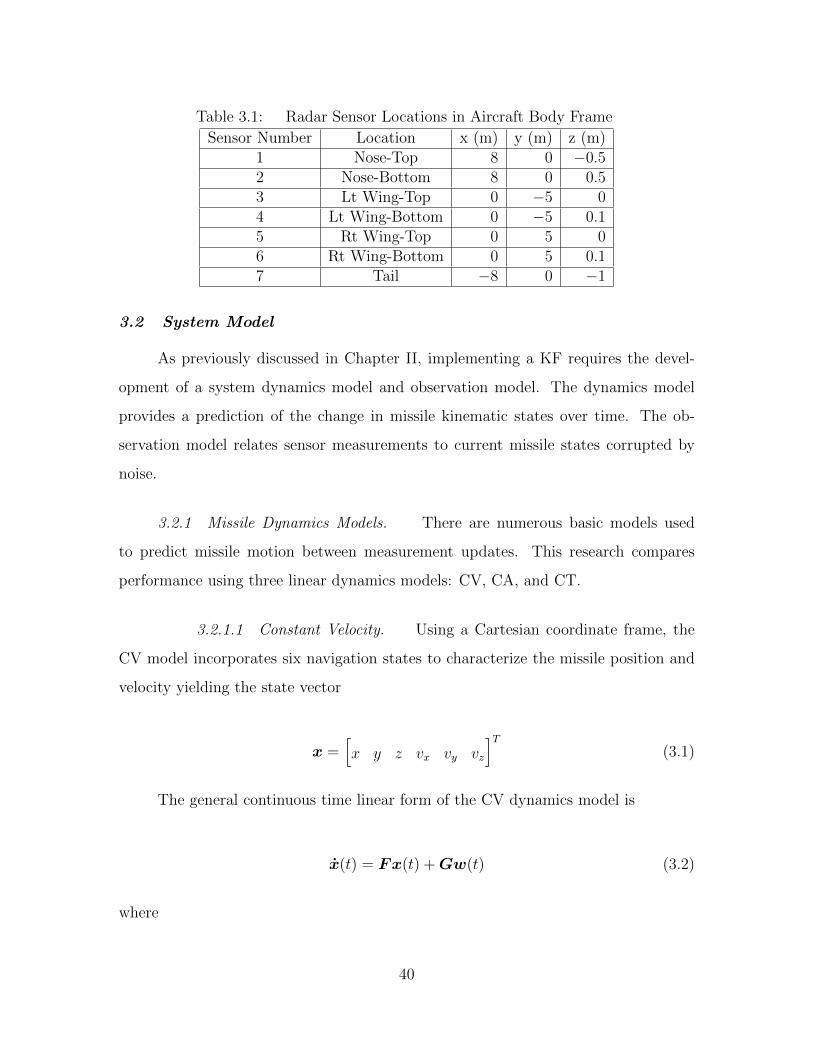
Table 3.1: Radar Sensor Locations in Aircraft Body Frame

Sensor Number Location x (m) y (m) z (m)1 Nose-Top 8 0 −0.52 Nose-Bottom 8 0 0.53 Lt Wing-Top 0 −5 04 Lt Wing-Bottom 0 −5 0.15 Rt Wing-Top 0 5 06 Rt Wing-Bottom 0 5 0.17 Tail −8 0 −1

3.2 System Model

As previously discussed in Chapter II, implementing a KF requires the devel-

opment of a system dynamics model and observation model. The dynamics model

provides a prediction of the change in missile kinematic states over time. The ob-

servation model relates sensor measurements to current missile states corrupted by

noise.

3.2.1 Missile Dynamics Models. There are numerous basic models used

to predict missile motion between measurement updates. This research compares

performance using three linear dynamics models: CV, CA, and CT.

3.2.1.1 Constant Velocity. Using a Cartesian coordinate frame, the

CV model incorporates six navigation states to characterize the missile position and

velocity yielding the state vector

x =[x y z vx vy vz

]T(3.1)

The general continuous time linear form of the CV dynamics model is

x(t) = Fx(t) +Gw(t) (3.2)

where

40

F =

03x3 I3x3

03x3 03x3

(3.3)

G =

03x3

I3x3

(3.4)

and the strength of the noise vector w(t) is defined by

E[w(t)w(t+ τ)] = Q =

q 0 0

0 q 0

0 0 q

(3.5)

The variable q is adjusted during filter tuning to improve performance.

In an inertial reference frame, the CV model assumes a constant velocity along

each axis while acceleration along each axis is modeled by an independent, zero-mean,

Gaussian, white noise. For this research the propagation time steps are in milliseconds,

and the missile is tracked for a short duration of a couple seconds. Therefore, a flat

Earth is assumed and missile propagation is performed in a local-level navigation

frame with an origin on the surface of the Earth (i.e. n-frame approximates i-frame).

Converting the dynamics model into discrete time, the general form for the

difference equation is

xk = φxk−1 +Gwk−1 (3.6)

This result is similar to Equation (2.12) except the deterministic input, uk is zero for

this estimation problem. Applying the Van Loan [7] method to solve for the state

transition matrix, φ, and the noise strength matrix, Qd, yields [5]

41

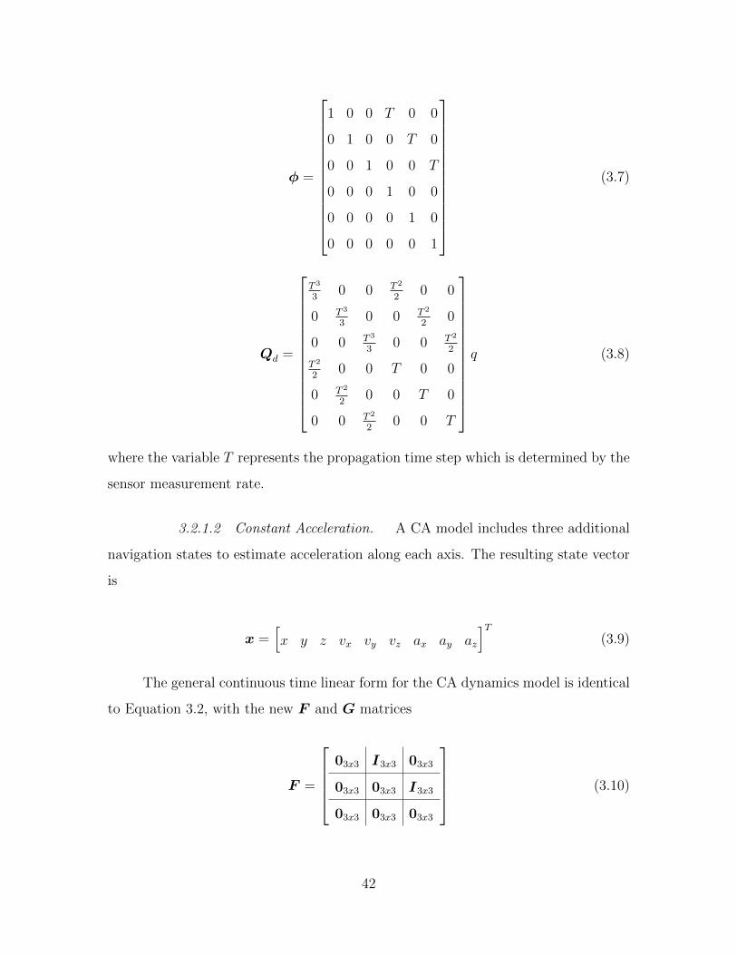
φ =

1 0 0 T 0 0

0 1 0 0 T 0

0 0 1 0 0 T

0 0 0 1 0 0

0 0 0 0 1 0

0 0 0 0 0 1

(3.7)

Qd =

T 3

30 0 T 2

20 0

0 T 3

30 0 T 2

20

0 0 T 3

30 0 T 2

2

T 2

20 0 T 0 0

0 T 2

20 0 T 0

0 0 T 2

20 0 T

q (3.8)

where the variable T represents the propagation time step which is determined by the

sensor measurement rate.

3.2.1.2 Constant Acceleration. A CA model includes three additional

navigation states to estimate acceleration along each axis. The resulting state vector

is

x =[x y z vx vy vz ax ay az

]T(3.9)

The general continuous time linear form for the CA dynamics model is identical

to Equation 3.2, with the new F and G matrices

F =

03x3 I3x3 03x3

03x3 03x3 I3x3

03x3 03x3 03x3

(3.10)

42

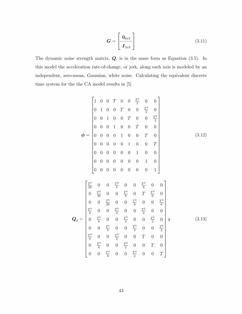
G =

06x3

I3x3

(3.11)

The dynamic noise strength matrix, Q, is in the same form as Equation (3.5). In

this model the acceleration rate-of-change, or jerk, along each axis is modeled by an

independent, zero-mean, Gaussian, white noise. Calculating the equivalent discrete

time system for the the CA model results in [5]

φ =

1 0 0 T 0 0 T 2

20 0

0 1 0 0 T 0 0 T 2

20

0 0 1 0 0 T 0 0 T 2

2

0 0 0 1 0 0 T 0 0

0 0 0 0 1 0 0 T 0

0 0 0 0 0 1 0 0 T

0 0 0 0 0 0 1 0 0

0 0 0 0 0 0 0 1 0

0 0 0 0 0 0 0 0 1

(3.12)

Qd =

T 5

200 0 T 4

80 0 T 3

60 0

0 T 5

200 0 T 4

80 T T 3

60

0 0 T 5

200 0 T 4

80 0 T 3

6

T 4

80 0 T 3

30 0 T 2

20 0

0 T 4

80 0 T 3

30 0 T 2

20

0 0 T 4

80 0 T 3

30 0 T 2

2

T 3

60 0 T 2

20 0 T 0 0

0 T 3

60 0 T 2

20 0 T 0

0 0 T 3

60 0 T 2

20 0 T

q (3.13)

43

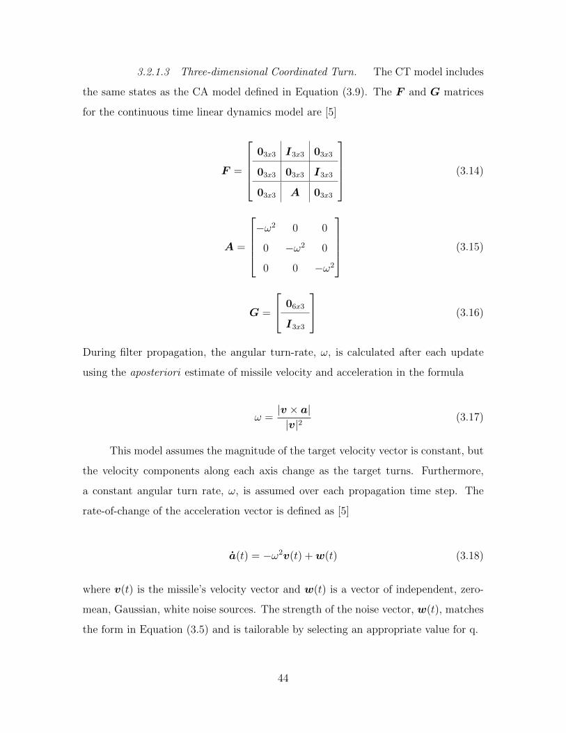
3.2.1.3 Three-dimensional Coordinated Turn. The CT model includes

the same states as the CA model defined in Equation (3.9). The F and G matrices

for the continuous time linear dynamics model are [5]

F =

03x3 I3x3 03x3

03x3 03x3 I3x3

03x3 A 03x3

(3.14)

A =

−ω2 0 0

0 −ω2 0

0 0 −ω2

(3.15)

G =

06x3

I3x3

(3.16)

During filter propagation, the angular turn-rate, ω, is calculated after each update

using the aposteriori estimate of missile velocity and acceleration in the formula

ω =|v × a||v|2 (3.17)

This model assumes the magnitude of the target velocity vector is constant, but

the velocity components along each axis change as the target turns. Furthermore,

a constant angular turn rate, ω, is assumed over each propagation time step. The

rate-of-change of the acceleration vector is defined as [5]

a(t) = −ω2v(t) +w(t) (3.18)

where v(t) is the missile’s velocity vector and w(t) is a vector of independent, zero-

mean, Gaussian, white noise sources. The strength of the noise vector, w(t), matches

the form in Equation (3.5) and is tailorable by selecting an appropriate value for q.

44

In discrete time, the CT model state transition matrix is a function of ω as

described by [5]

φ(ω) =

A(ω) 03x3 03x3

03x3 A(ω) 03x3

03x3 03x3 A(ω)

(3.19)

where A(ω) is defined as

A(ω) =

1 sinωT

ω1−cosωT

ω2

0 cosωT sinωTω

0 −ω sinωT cosωT

(3.20)

The closed form solution for the CT model’s discrete noise strength, Qd, is intention-

ally omitted due to complexity. However, given a value of ω, the numerical solution

is relatively straight forward by application of the Van Loan method described in

Chapter II. The interested readers is referred to [5] for details.

3.2.2 Observation Model. Range and range-rate measurements are a non-

linear function of system states. Therefore, this research utilizes a nonlinear measure-

ment model with a vector of independent, additive, zero-mean, Gaussian, white noise

sources in the general form of Equation 2.19 [18].

The range measurement from the i -th sensor is related to the system states

according to

ri =√

(x− xi)2 + (y − yi)2 + (z − zi)2 (3.21)

The sensor coordinates, [xi yi zi], are easily defined in the aircraft body frame, but

must be converted into the same reference frame as the missile state vector. In this

research, the missile state vector is expressed in a local level Earth-fixed navigation

45

frame. In addition, radar radial velocity measurements from the i -th sensor are

defined by

vi = −(vx − vxi)(x− xi) + (vy − vyi)(y − yi) + (vz − vzi)(z − zi)√(x− xi)2 + (y − yi)2 + (z − zi)2

(3.22)

3.3 Gating and Data Association Implementation

The radar sensors for the missile scoring system are unlikely to see a large

number of false returns in their operating environment for several reasons. First of

all, the FMCW sensors are short range so the volume of airspace they observe is

extremely limited. Secondly, a drone aircraft equipped with a missile scoring system

for missile test and evaluation is generally operated in visual meteorological conditions

for safety. However, the algorithm used in this research does include two features to

limit the impact of false radar returns: gating and data association.

Square and ellipsoidal gating are applied sequentially as described in Section 2.8.

Since multiple sensors are employed for this end-game missile scoring system, gating

is applied to measurements from each sensor separately. If multiple measurements

from a single sensor survive gating then GNN data association is applied as outlined

in Section 2.8.

3.4 Target Initialization

The nonlinear KF algorithms used in this research are initialized by simulating

missile position and velocity information from an external source. Most air-to-air

missile test and evaluation ranges include a system which monitors missile position

for safety. For example, missile testing performed at Tyndall Air Force Base (AFB)

utilizes the Gulf range drone control system (GRDCS) [16]. This system provides

position accuracy of approximately 15 meters in the x and y-axis and 45 meters in

the z-axis. The data update rate is 20 Hz and velocity is determined by calculating the

change in position over one time step. Based on the GRDCS system the missile state

vector is set equal to truth with a random position and velocity error added to each

46

axis from a zero-mean normal distribution with the following standard deviations:

σx = 15, σy = 15, σz = 45, σvx = 10, σvy = 10 and σvz = 10. Furthermore, the initial

covariance matrix is set according to the GRDCS uncertainty as

P0 =

σ2x 0 0 0 0 0

0 σ2y 0 0 0 0

0 0 σ2z 0 0 0

0 0 0 σ2vx 0 0

0 0 0 0 σ2vy 0

0 0 0 0 0 σ2vz

(3.23)

An alternate approach is to initialize the target purely based on sensor mea-

surements through multilateration as described in Section 2.6. A downside to this

approach is it requires four measurements. If target detection probability is low, the

multilateration procedure will not have sufficient information to initialize the target

state vector [10]. Alternatively, if the sensors see large numbers of ghost targets, the

multilateration process requires the tracking of multiple target hypotheses. Track

scoring is one possible technique for making decisions on which track is the true tar-

get [5]. However, in a multiple target and high clutter environment this approach

becomes computationally burdensome. Fortunately, in target scoring applications

with short range sensors, a low clutter environment is probable.

3.5 Nonlinear Kalman Filter Implementation

As explained in Section 2.4, a conventional KF is inadequate to deal with the

nonlinearities present in the system observation model. When performing estimation

of nonlinear systems there is no single optimal approach for all problems. Some

nonlinear filters may have an advantage in computational burden while another has

superior precision or reduced complexity. Therefore, three different nonlinear Kalman

filters are implemented in this research: an EKF, UKF, and PF. In Chapter IV their

performance is compared to assess advantages when utilized in an end-game missile

47

scoring system. Appendix C includes the computer algorithms developed for this

research. This software includes the main EKF, UKF, and PF programs along with

all associated subprograms for performing the simulations detailed in Chapter IV.

Since all of the dynamics models considered in this research are linear, con-

ventional KF Equations (2.14)-(2.16) are applied to propagate the state estimates in

both the EKF and UKF filters. The PF uses a slightly different approach as outlined

previously in Section 2.4.3.

3.5.1 Extended Kalman Filter. An EKF deals with nonlinearities in a system

observation model by linearizing about a nominal measurement using a first-order

Taylor series approximation. In order to linearize the observation model a Jacobian

matrix is calculated as described in Section 2.4.1. The matrix is then evaluated at

the apriori estimate according to Equation (2.20). For this end-game missile scoring

application, when utilizing the CV missile dynamics model, the resulting H matrix is

in the form

H =

δriδx

δriδy

δriδz

δriδvx

δriδvy

δriδvz

δviδx

δviδy

δviδz

δviδvx

δviδvy

δviδvz

(3.24)

For the more complex nine state Kalman filters based on the CA or CT dynamics

model, the general form of the H matrix is

H =

δriδx

δriδy

δriδz

δriδvx

δriδvy

δriδvz

δriδax

δriδay

δriδaz

δviδx

δviδy

δviδz

δviδvx

δviδvy

δviδvz

δviδax

δviδay

δviδaz

(3.25)

The partial derivatives of Equations (3.21) and (3.22) used to populate the H matrix

are summarized below [36] 1:

1The expressions ri and vi are substituted wherever possible to keep the length of the equationsmanageable.

48

δriδx

=x− xiri

(3.26)

δriδy

=y − yiri

(3.27)

δriδz

=z − ziri

(3.28)

δriδvx

=δriδvy

=δriδvz

= 0 (3.29)

δriδax

=δriδay

=δriδaz

= 0 (3.30)

δviδx

= −vi(x− xi)r2i

− vx − vxiri

(3.31)

δviδy

= −vi(y − yi)r2i

− vy − vyiri

(3.32)

δviδz

= −vi(z − zi)r2i

− vz − vziri

(3.33)

δviδvx

= −x− xiri

(3.34)

δviδvy

= −y − yiri

(3.35)

δviδvz

= −z − ziri

(3.36)

49

δviδax

=δviδay

=δviδaz

= 0 (3.37)

Next, nominal range and radial velocity measurements for each sensor are calcu-

lated by evaluating Equations (3.21) and (3.22) at the apriori estimate. As noted in

Section 3.2.2, the coordinates of the sensors must be converted into the same reference

frame as the missile state vector.

The perturbation state vector, δz, contains the difference between the realized

sensor measurements of range and radial velocity and the nominal. The size of δz is

dependent on the number of sensors with measurements that survive the gating pro-

cess. For example, if sensors one and three detect the target and these measurements

survive gating the resulting perturbation state vector is a four-by-one in the general

form

δz =

δr1

δv1

δr3

δv3

(3.38)

where δri represents the difference between the i -th sensor realized range measurement

and calculated nominal measurement. Similarly, δvi is the difference between the i -th

sensor realized radial velocity measurement and nominal. A common discrete time

subscript, k, is implied in Equations (3.24)-(3.38) and is intentionally omitted to avoid

confusion with the sensor number subscript.

Finally, the aposteriori state estimate, x+k , and uncertainty, P+

k are updated

using the resulting H matrix and perturbation state vector according to Equa-

tions (2.16), (2.18) and (2.23).

3.5.2 Unscented Kalman Filter. Section 2.4.2 describes the UKF algorithm

in detail. For this research, the initial sigma points locations are calculated after time

50

propagation using Equations (2.24)-(2.28). The scaling factor, λ, is determined by

setting the tuning parameters α and κ to 0.1 and zero, respectively.

Next, each sigma point is transformed into observation space by evaluating

Equations (3.21)-(3.22) at their respective location. To clarify, each sigma point is a

representation of the missile state vector (i.e., the weighted sum of all sigma points is

the estimate of the state vector). Therefore, the missile location, [x y z], and velocity,

[vx vy vz], needed to evaluate Equations (3.21)-(3.22) comes directly from rows one

through six of each sigma point.

After transforming all of the sigma points, a measurement prediction and uncer-

tainty are calculated for the i -th sensor using Equations (2.30)-(2.34). Gating is then

applied to the measurements from each sensor. The best surviving measurement from

each sensor, as defined by GNN data association, is saved for missile state update.

In addition, the transformed sigma points, Z , from sensors with surviving measure-

ments are saved for performing the aposteriori update. For example, if measurements

are saved from sensors three and seven, the measurement vector, z, is of the form

z =

r3

v3

r7

v7

(3.39)

and Z ∈ R4×2L+1, where L is the number of missile states. Finally, the surviving

measurements are used to calculate the aposteriori state estimate and uncertainty via

Equations (2.30)-(2.38). Discrete time subscripts are again omitted in this section for

clarity.

3.5.3 Particle Filter. Implementation of the PF is similar to the UKF. As

discussed in Section 2.4.3, sample points replace the sigma points for representing

the pdf of the missile state vector. For this application, the initial sample points are

generated when the filter is initialized using data from the GRDCS. Equation (2.39) is

51

used to randomly generate the initial particle locations and all particles are weighted

equally according to Equation (2.41).

Propagation of the missile state estimate in the PF is accomplished by trans-

forming each particle through the linear dynamics function as illustrated in Equa-

tion (2.42). Random noise, consistent with the statistics of the noise sources in the

dynamics model, is added to each particle as described in Section 2.4.3. As a result

of particle propagation, the location of each particle changes while its weight remains

the same. The aprior state estimate and uncertainty is determined from resulting

particle locations as outlined in Equations (2.44) and (2.45).

Measurement updates for the PF are performed in an analogous fashion to the

UKF. Each particle is transformed through Equations (3.21) and (3.22). The trans-

formed particles are used to predict each sensor’s measurement and the associated

uncertainty. Gating is then applied to eliminate unlikely measurements from each

sensor and the closest remaining measurements and associated particles are saved for

state update. To perform the aposteriori update, the saved measurements are applied

to adjust the particle locations and weights according to Equations (2.47)-(2.51). Fi-

nally, the updated state estimate, x+k , and uncertainty, P+

xk, are calculated from the

new particle locations and weights using Equations (2.44) and (2.45).

Unfortunately, this application requires a large quantity of particles to avoid par-

ticle starvation. Particle starvation is often an issue in particle filters with uncertain

dynamics models (i.e., large system noise, Q) and highly precise sensor measurements

(i.e., low sensor noise, R). When a measurement update is performed, the weights of

particles are adjusted based on their likelihood given the measurement realization ac-

cording to Equations (2.48)-(2.50). A large ratio of system noise to sensor noise often

results in the majority of the particles having zero weight. The resulting statistics for

the missile state vector may be based on an insufficient number of particles and filter

divergence may occur.

52

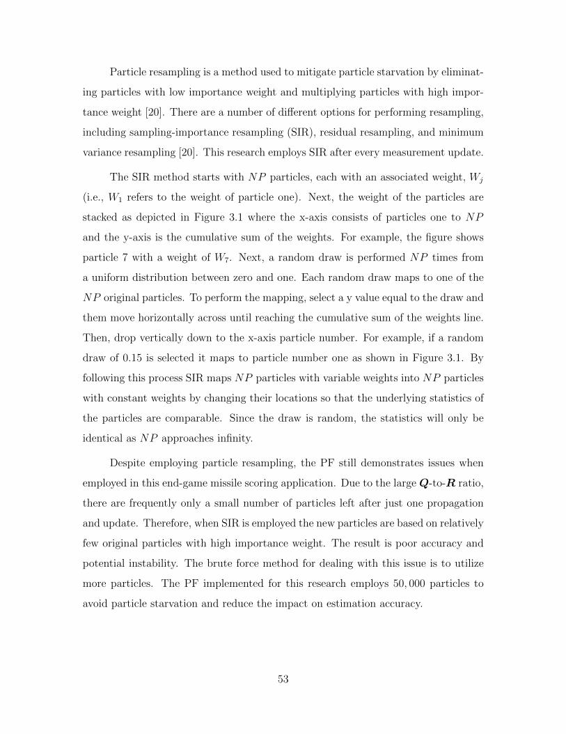
Particle resampling is a method used to mitigate particle starvation by eliminat-

ing particles with low importance weight and multiplying particles with high impor-

tance weight [20]. There are a number of different options for performing resampling,

including sampling-importance resampling (SIR), residual resampling, and minimum

variance resampling [20]. This research employs SIR after every measurement update.

The SIR method starts with NP particles, each with an associated weight, Wj

(i.e., W1 refers to the weight of particle one). Next, the weight of the particles are

stacked as depicted in Figure 3.1 where the x-axis consists of particles one to NP

and the y-axis is the cumulative sum of the weights. For example, the figure shows

particle 7 with a weight of W7. Next, a random draw is performed NP times from

a uniform distribution between zero and one. Each random draw maps to one of the

NP original particles. To perform the mapping, select a y value equal to the draw and

them move horizontally across until reaching the cumulative sum of the weights line.

Then, drop vertically down to the x-axis particle number. For example, if a random

draw of 0.15 is selected it maps to particle number one as shown in Figure 3.1. By

following this process SIR maps NP particles with variable weights into NP particles

with constant weights by changing their locations so that the underlying statistics of

the particles are comparable. Since the draw is random, the statistics will only be

identical as NP approaches infinity.

Despite employing particle resampling, the PF still demonstrates issues when

employed in this end-game missile scoring application. Due to the large Q-to-R ratio,

there are frequently only a small number of particles left after just one propagation

and update. Therefore, when SIR is employed the new particles are based on relatively

few original particles with high importance weight. The result is poor accuracy and

potential instability. The brute force method for dealing with this issue is to utilize

more particles. The PF implemented for this research employs 50, 000 particles to

avoid particle starvation and reduce the impact on estimation accuracy.

53

Particle Number

Cumulative Weights Sum

7

1

1

0.15

Figure 3.1: Sampling-Importance Resampling Procedure

Unfortunately, increasing particle numbers results in inefficiency and large com-

putational burden. A 100 run Monte Carlo simulation using a PF with 50, 000 parti-

cles takes approximately 48 mins and 9 seconds2. In contract, the EKF and UKF fil-

ters perform a 100 run Monte Carlo simulation in approximately 8.7 and 10.5 seconds,

respectively. An alternative to increasing the particle number is available through the

application of either an extended particle filter (EPF) or a unscented particle fil-

ter (UPF) [20]. The basic concept is to apply a bank of N EKF or UKF filters to

move particles from low likelihood regions into high likelihood regions based on the

measurement realization. This approach is not explored further in this research, but

Merwe, Doucet, Freitas and Wan provide a comprehensive discussion on the EPF and

UPF, including algorithms for implementation [20].

2Result based on the average execution time across all three scenarios described in Chapter IVusing a CV dynamics model. The simulations are performed on a Macbook with a 2.13 GHz IntelCore 2 Duo processor.

54

3.6 Summary

This chapter documented the methodology applied to implement the proposed

air-to-air missile scoring system. First, sensor placement on the drone aircraft was ad-

dressed and locations were proposed with justification. Next, three missile dynamics

models were derived for implementation within the Kalman filter algorithm: a CV,

CA, and CT. Also, the observation model was presented as a function of missile states

based on the available sensor measurements of range and range-rate. The remainder

of the chapter described the specific implementation of the three nonlinear Kalman

filter algorithms: an EKF, UKF, and PF. The description included an explanation

of the target initialization process and a discussion of gating and data association

implementation. The final section of this chapter compares the processing speed of

the three Kalman filter algorithms for the missile scoring application and foreshadows

the topic of the next chapter. The next chapter provides the methodology and results

from simulations designed to assess the overall performance of the scoring system and

compare the three proposed missile dynamics models and Kalman filter algorithms.

55

IV. Simulations

The proposed missile scoring solution is tested in three simulated scenarios to establish

performance. Scenario 1 is a non-maneuvering target attacked vertically from below.

Scenario 2 involves a tail-aspect attack against an aware adversary performing an

aggressive 9G descending break-turn into the shooter. Scenario 3 is also a tail-aspect

attack, but the target performs a 7G vertical maneuver. Section 4.1 discusses the

scenarios in greater detail. Section 4.2 describes the truth model used to generate the

scenarios and assess scoring performance.

A systematic approach to filter tuning is applied across all of the nonlinear fil-

ters evaluated in this research. Furthermore, target initialization error and sensor

noise is randomly generated for each scenario and for each Monte Carlo run and then

saved, so the same noise realization is used in all nonlinear filters. In other words,

during the 100 run Monte Carlo analysis, each filter method is subjected to the same

set of 100 sample functions of noise and 100 random initial hand-off errors. This

approach insures valid conclusions are drawn when comparing the performance of dif-

ferent missile dynamics models and nonlinear Kalman filters. Section 4.3 outlines the

tuning process and explains the justification behind the procedure. Section 4.4 pro-

vides samples of the randomly generated noise realizations to demonstrate statistical

properties (i.e., sensor and initialization errors are shown to be normally distributed

with desired mean and standard deviation).

Sections 4.5 and 4.6 compare the results from simulations to draw conclusions

about which nonlinear KF and dynamics model provide the greatest precision in

missile state estimates at impact. Since this research considers three scenarios, three

dynamics models, and three nonlinear Kalman filters, there are a total of 27 simulation

combinations. Only the highlights are addressed in this chapter, but Appendix A

includes a comprehensive record of simulation results. All of the simulations consist

of a 100 run Monte Carlo analysis where error mean and standard deviation are

plotted for each of the missile position and velocity states.

56

Section 4.7 concludes this chapter by assessing the performance of the the best

nonlinear KF and dynamics model combination from those considered in this research.

4.1 Scenarios

Figure 4.1 depicts the flight profile for scenario 1. The target aircraft is wings-

level, flying northbound at an altitude of 5000 meters and does not maneuver for the

duration of the missile intercept. The shooter starts from a position one mile in front

of the target on a southbound heading, at an altitude of 500 meters and a 70 degree

pitch-up attitude. The true aircraft and missile trajectory are depicted for the entire

simulation of approximately eight seconds.

Figure 4.2 illustrates the aircraft and missile 3D trajectory for scenario 2. The

drone aircraft begins the simulation in a wings-level attitude, heading north, at an

altitude of 5000 meters. After the simulation starts, the target rolls to approximately

120 degrees of bank and initiates a 9G, right-hand, descending turn. This break-turn

maneuver is a common defensive tactic employed by an aircraft when targeted by a

missile within visual range. Missile impact occurs as the target is passing through an

easterly heading at an altitude of about 4300 meters. The shooter fires at the outset

−1500−1000

−5000

5001000

1500

0

500

1000

1500

2000

2500

30000

1000

2000

3000

4000

5000

East(+)/West(−) (m)North(+)/South(−) (m)

Alti

tude

(m

)

Aircraft Start PositionAircraft TrajectoryMissile Start PositionMissile True TrajectoryMissile Estimate

Figure 4.1: Scenario 1: Target Aircraft Non-maneuvering

57

−2000

200400

600800

1000

−2000

−1000

0

1000

20003500

4000

4500

5000


Alti

tude

(m

)Aircraft Start PositionAircraft TrajectoryMissile Start PositionMissile True TrajectoryMissile Estimate

Figure 4.2: Scenario 2: Target Aircraft Performing a 9G Descending Break-Turn

of the scenario from a three mile trail position, heading north, at an altitude of 5000

meters.

In scenario 3 the target starts the simulation wings-level, northbound, at an

altitude of 5000 meters as shown in Figure 4.3. The shooter starts out two miles in

trail with attitude and altitude identical to the target. When the simulation begins,

the drone aircraft performs a 7G vertical pull-up while the shooter immediately fires.

−1000

−500

0

500

1000

−3000

−2000

−1000

0

10005000

5100

5200

5300

5400

5500


Alti

tude

(m

)


Figure 4.3: Scenario 3: Target Aircraft Performing a Vertical Climb

58

4.2 Truth Model

In order to provide realistic missile truth data in the presented dynamic sce-

narios, two separate simulation tools are employed: Profgen and Argos 3.0. Profgen

takes a vehicle through a series of maneuvers to produce kinematic outputs. These

kinematic outputs, which track the motion of an aircraft in six degrees-of freedom

(6DOF), provide target information for use in Argos. Argos is a 6DOF missile sim-

ulation tool developed through collaboration between the National Air and Space

Intelligence Center (NASIC) and the Air Force Research Laboratories (AFRL).

In Profgen [25], the user specifies the dynamic capabilities of the vehicle and

directs maneuvers by stringing together basic profile elements such as horizontal and

vertical turns, jinks, accelerations, and rolls. Since only the kinematic solution is of

interest, Profgen models the vehicle as a point-mass body and considerations such as

lift, drag, weight, and thrust are substantially reduced. Profgen outputs are specified

in one of two coordinate frames, World Geodetic System 1984 (WGS 84) or Standard

Navigation Unit, with five associated reference frames: inertial, Earth-centered Earth-

fixed (ECEF), geodetic, wander-level, and body.

In this research, aircraft data is output in a WGS-84 ECEF reference frame and

then externally converted into a local-level Earth-centered NED navigation frame

for import into Argos and our nonlinear KF algorithms. Argos only utilizes target

aircraft position and velocity information to compute missile trajectory. In contrast,

the Kalman filters requires truth data on aircraft attitude in addition to position and

velocity.

Argos [3] provides numerous options for missile models and coordinate frames

for performing simulations. The simulation results in this research are obtained using

an unclassified short-range missile and assuming a flat-Earth environment. The sim-

ulation is based in Matlab simulink and the resulting missile kinematic data is output

in a NED local-level navigation frame. The true missile position is not known to the

59

filter, but it’s used to generate noise corrupted sensor measurements and compute

filter error.

4.3 Filter Tuning

The filter tuning is performed during scenario 2 because it represents the most

dynamic scenario based on the degree of target maneuvers. Since the filer is required

to operate without prior knowledge of the aircraft and missile profile, each filter’s

tuning parameters are held constant over all three scenarios. Four different param-

eters are varied during the tuning process: gate size, γ, dynamic noise strength, q,

and two values in the observation noise strength matrix, R. The sensor range and

velocity noise are assumed to be uncorrelated, so the R matrix from a single sensor

measurement is in the general form

R =

rrange 0

0 rvelocity

(4.1)

where rrange represents the uncertainty associated with sensor range measurements

and rvelocity is the uncertainty in sensor velocity measurements. These variables are

adjusted independently during the tuning process.

Tuning is initially conducted on the EKF filter using the CV dynamics model.

The starting point for the adjustable parameters is selected based on an understanding

of how each variable effects the estimation process along with knowledge of actual

sensor characteristics. For example, a gamma value of 9.8 is an excellent initial guess

because it insures that 99 percent of the true measurements will fall within the confines

of ellipsoidal gating. In addition, sensor range measurement errors are 2.5 percent of

target range while expected velocity measurement errors are just 0.25 meters per

second. Therefore, rrange is an order of magnitude higher than rvelocity at a target

range of 100 meters.

60

Based on this preliminary knowledge, multiple trials are conducted to assess the

EKF filter parameters that provide the best position and velocity precision during

scenario 2 using a 100 run Monte Carlo analysis. The result for the CV missile

dynamics model is γ = 20, q = 1, 000, rrange = 10, and rvelocity = 2. The large increase

in gate size is not surprising since clutter measurements are low density and uniformly

distributed. Therefore, there’s a low probability that a clutter measurement will be

incorporated into the missile state estimate even with a larger gamma value. As a

result, using a larger gamma value provides the benefit of increasing the likelihood

that true measurements survive gating without a significant risk of false measurements

impacting missile state estimates. The dynamics noise value of 1,000 may appear large

relative to R, but converting to a discrete dynamics noise strength matrix based on

a time step of 10 milliseconds results in

Qd =

0.0003 0 0 0.0500 0 0

0 0.0003 0 0 0.0500 0

0 0 0.0003 0 0 0.0500

0.0500 0 0 10 0 0

0 0.0500 0 0 10 0

0 0 0.0500 0 0 10

(4.2)

When performing filter tuning for different missile dynamics models, only the

parameter for dynamics noise strength is adjusted. This varying of q places a different

weight on the missile dynamics model when performing estimations of missile position

and velocity. Under this limitation, EKF filter tuning is accomplished for the CA and

CT missile models yielding q = 500, 000 and q = 800, 000, respectively.

Since all of the nonlinear Kalman filters utilize identical dynamics and observa-

tion models, the same filter tuning parameters determined for the EKF are initially

applied to the UKF and PF to facilitate performance comparison. This technique

works well with the UKF, however, the PF exhibits instability due to particle star-

vation. As discussed in Section 3.5.3, particle starvation is exacerbated by highly

61

accurate measurements in the face of uncertain dynamics. In order to avoid this

problem while keeping particle numbers to a reasonable level for simulation time con-

straints, rrange and rvelocity are both increased to 20. Table 4.1 summarizes the tuning

parameters used in each filter.

Table 4.1: Summary of Nonlinear Kalman Filter Tuning Parameters

Filter-Dynamics Model γ q rrange rvelocityEKF-CV 20 1,000 10 2EKF-CA 20 500,000 10 2EKF-CT 20 800,000 10 2UKF-CV 20 1000 10 2UKF-CA 20 500,000 10 2UKF-CT 20 800,000 10 2

PF-CV (50,000 Particles) 20 1000 20 20PF-CA (50,000 Particles) 20 500,000 20 20PF-CT (50,000 Particles) 20 800,000 20 20

4.4 Noise Generation

During simulations the missile state estimates are affected by randomly gen-

erated noise from three general areas. First, there is noise impacting the sensor

measurements of range and radial velocity. Second, there are clutter measurements

from false returns picked up by the sensors. Third, the initial target state vector

contains random errors based on handoff from the GRDCS.

During algorithm testing, radar clutter is simulated separately for each sen-

sor. During each measurement update, individual sensors return observations based

upon the true missile position as well as clutter. The true (noise corrupted) obser-

vations are generated from truth data by adding random noise from a zero-mean,

Gaussian distribution with variance defined by the sensor performance as described

in Section 3.1. For clutter, the number of false observations are chosen from random,

uniformly distributed integers over the interval [0,3]. Each clutter measurement takes

on a value chosen from a random, uniform distribution over the sensor’s minimum

detection range and range-rate through its maximum detection range and range-rate.

62

In other words, false returns are modeled uniformly within the sensor volume rather

than simulating clutter returns from multiple parts of the missile.

In order to guarantee valid comparisons between the various filter-missile model

combinations, two of the three noise areas are seeded such that all filter-missile models

see the same noise realizations for a specific run of a given scenario. The radar clutter

is the only noise area not seeded because gating effectively eliminates its impact on

the missile state estimates. To perform seeding, the sensor and initialization noise

is randomly generated according to desired statistical properties during EKF-CV

simulations for each of the three scenarios. This data is then saved so the other eight

filter-missile model combinations use identical noise.

Figure 4.4 illustrates the statistical properties of the sensor noise from a single

sensor during scenario 1. The histograms in Figures 5.4(a) and 5.4(b) depict the

number of sensor noise values in each bin for sensor range and radial velocity mea-

surements, respectively. The dashed line plots overlaid on the histograms illustrate

the desired Gaussian distribution for comparison. In Figure 5.4(a) it is important to

note the noise realizations are actually scaling values since sensor precision is based on

target range (i.e., a value of 0.01 indicates the actual noise realization is one percent

of the true range).

−0.05 −0.04 −0.03 −0.02 −0.01 0 0.01 0.02 0.03 0.04 0.050

100

200

300

400

500

600

Noi

se R

ealiz

atio

ns in

Bin

Sensor Range Measurement Noise Scaling Value

(a) Sensor Range Noise Realization

−0.5 −0.4 −0.3 −0.2 −0.1 0 0.1 0.2 0.3 0.4 0.50

100

200

300

400

500

600

Noi

se R

ealiz

atio

ns in

Bin

Sensor Velocity Measurement Noise Value (m/s)

(b) Sensor Velocity Noise Realization

Figure 4.4: Statistical Properties of Random Sensor Noise Realization Utilized forall Scenario 1 Simulations

63

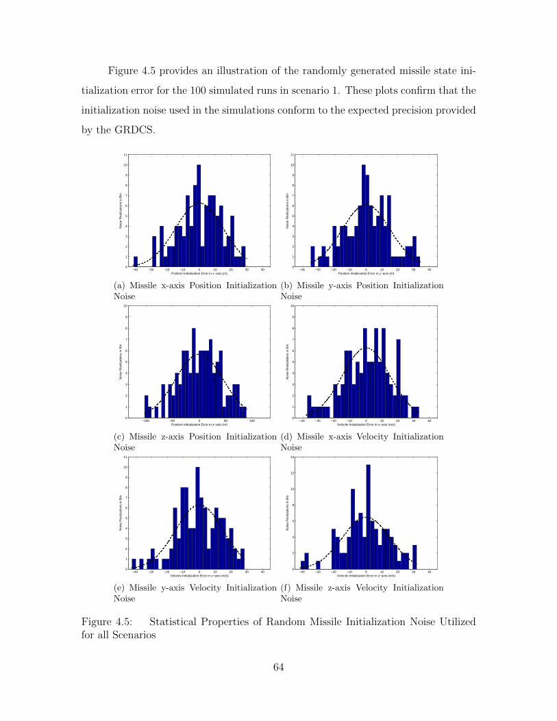
Figure 4.5 provides an illustration of the randomly generated missile state ini-

tialization error for the 100 simulated runs in scenario 1. These plots confirm that the

initialization noise used in the simulations conform to the expected precision provided

by the GRDCS.

−40 −30 −20 −10 0 10 20 30 400

1

2

3

4

5

6

7

8

9

10

11

Noi

se R

ealiz

atio

ns in

Bin

Position Initialization Error in x−axis (m)

(a) Missile x-axis Position InitializationNoise

−40 −30 −20 −10 0 10 20 30 400

1

2

3

4

5

6

7

8

9

10

11

Noi

se R

ealiz

atio

ns in

Bin

Position Initialization Error in y−axis (m)

(b) Missile y-axis Position InitializationNoise

−100 −50 0 50 1000

1

2

3

4

5

6

7

8

9

10

Noi

se R

ealiz

atio

ns in

Bin

Position Initialization Error in z−axis (m)

(c) Missile z-axis Position InitializationNoise

−40 −30 −20 −10 0 10 20 30 400

1

2

3

4

5

6

7

8

9

10

Noi

se R

ealiz

atio

ns in

Bin

Velocity Initialization Error in x−axis (m/s)

(d) Missile x-axis Velocity InitializationNoise

−40 −30 −20 −10 0 10 20 30 400

1

2

3

4

5

6

7

8

9

10

11

Noi

se R

ealiz

atio

ns in

Bin

Velocity Initialization Error in y−axis (m/s)

(e) Missile y-axis Velocity InitializationNoise

−40 −30 −20 −10 0 10 20 30 400

2

4

6

8

10

12

14

Noi

se R

ealiz

atio

ns in

Bin

Velocity Initialization Error in z−axis (m/s)

(f) Missile z-axis Velocity InitializationNoise

Figure 4.5: Statistical Properties of Random Missile Initialization Noise Utilizedfor all Scenarios

64

For example, in Figures 5.5(a) and 5.5(b) the x and y axis position error histogram

approximates a normal distribution with a standard deviation of 15 meters. The z-axis

position error plotted in Figure 5.5(c) follows a normal distribution with a standard

deviation of 45 meters. Finally, the velocity error in all axes has a standard deviation

of 15 meters per second.

4.5 Dynamics Model Comparison

Of the three dynamics models evaluated, the CV provides the best performance

in terms of precision. The precision is assessed by evaluating the missile state er-

ror standard deviation at missile impact over a 100 run Monte Carlo analysis. All

simulations assume a 10 millisecond sensor measurement rate. Furthermore, the sen-

sor measurements all occur simultaneously based on a common clock. According to

the simulation results for the EKF and PF, the CV model exhibited a smaller stan-

dard deviation in at least five of the six missile navigation states at impact across

all scenarios tested. Table 4.2 provides a sample of the results obtained for the EKF

in Scenario 2, where initial filter tuning is conducted (see Appendix A for complete

simulation results).

The worst case position precision for scenario 2 appears in the z-axis where

the CV model exhibits an error standard deviation of 11.3 centimeters at impact.

In comparison, the alternate dynamics models are significantly worse at 19.83 and

Table 4.2: Comparison of Missile State Estimate Error Standard Deviation atImpact for Different Dynamics Models using an Extended Kalman Filter (Sce-nario 2)Missile State CV Model Error CA Model Error CT Model Error

Standard Deviation Standard Deviation Standard Deviationx 0.0194 m 0.0224 m 0.0231 my 0.0762 m 0.1210 m 0.1099 mz 0.1130 m 0.1983 m 0.1671 mvx 0.9391 m

s1.9879 m

s2.3412 m

s

vy 6.2837 ms

12.9057 ms

9.1882 ms

vz 8.5262 ms

19.7077 ms

12.0386 ms

65

16.71 centimeters. Similarly, the worst velocity precision occurs in the z-axis for all

dynamics models. Once again, the CV model is much better with a standard deviation

of 8.5262 meters per second. The CA shows greater than a 100 percent reduction in

precision at 19.7077 meters per second. The CT models shows more than a 40 percent

decrease in precision at 12.0386 meters per second.

The simulation results for the UKF are inconsistent, showing marginally higher

precision with the CA dynamics models in about half of the missile states at impact.

However, this is likely the result of filter tuning. The UKF adopted the same tuning

parameters as the EKF and did not undergo independent tuning. One clear indication

that the CV model provides better performance is revealed by examining the values

of q used in the dynamics noise matrix for the different models. Filter tuning on the

EKF-CV resulted in a q value of 1,000. In contrast, the CA and CT models used

q values of 500,000 and 800,000, respectively. The large increase in q is effectively

telling the filter to place less trust in the dynamics model and more faith in the

measurements. In fact, q is so high that the filter is almost entirely ignoring the

dynamics model.

The CV model also provides an advantage in simplicity and speed. Both the

CA and CT model require the estimation of missile state acceleration in addition

to position and velocity. These nine state filters result in increased computational

complexity over the six state CV model. As a result, the CV filter algorithms will

execute faster, especially in the case of the PF.

These results are not surprising since the radar sensors update at the high rate

of 10 msec. Since the filter propagation intervals are so small, the missile velocity

remains relatively constant over each interval and the CV model closely approximates

missile dynamics.

66

4.6 Filter Comparison

An examination of the simulation results demonstrates the UKF is the ideal

choice for this missile scoring application based on superior precision. Tables 4.3-4.5

compare the missile state estimate error standard deviation of each nonlinear Kalman

filter for each of the three scenarios.

Table 4.3: Comparison of Missile State Estimate Error Standard Deviation atImpact for Different Nonlinear Kalman Filters (Scenario 1)Missile State EKF Error UKF Error PF Error


s4.7050 m

s10.6083 m

s

vy 9.4838 ms

8.0019 ms

19.3195 ms

vz 1.3355 ms

1.1521 ms

3.1860 ms



s0.5608 m

s2.6605 m

s

vy 6.2837 ms

2.4432 ms

9.4397 ms

vz 8.5262 ms

2.5532 ms

10.3529 ms



s0.5371 m

s1.8390 m

s

vy 11.8460 ms

8.4909 ms

20.8787 ms

vz 13.7464 ms

3.6732 ms

9.4543 ms

67

These results are all based on a CV dynamics model since it provides the best

performance. The UKF precision at missile impact outperforms the other Kalman

filters in 17 of 18 state estimates across the three scenarios.

4.7 Missile Scoring Performance

In order to assess the performance of the proposed missile scoring system, the

accuracy and precision of the UKF-CV is evaluated in each of the three simulated

scenarios. This filter-dynamics model combination is chosen based on its superior

precision and reduced complexity over the other options considered.

The results from scenario 1 are recorded in Figure 4.6. Figure 4.6(a) provides

a quick graphical reference of the flight profile covered in detail in Section 4.1 . The

missile estimate from the proposed scoring system is overlaid on this plot, but is only

depicted after the missile reaches the expected sensor range limit of 350 meters.

The Root Sum Square (RSS) position error for a single sample run is shown in

Figure 4.6(b). The target is randomly initialized for the sample run in accordance

with typical GRDCS range accuracies as discussed in Section 3.4. For the particular

run shown, the position error is initially about 48 meters and the estimate improves

to an end-game error on the order of centimeters. The continuous improvement in

the position accuracy as the missile closes on the target is a result of better sensor

geometry leading to improved observability of missile states. The final simulation

time corresponds to missile impact with the target.

In addition, a 100 run Monte Carlo analysis is performed to evaluate the errors

in the estimates of each of the six missile navigation states. Figures 4.6(c) and 4.6(d)

record the results and the statistics are summarized in Table 4.6.

Despite large initialization errors in position, the ensemble mean error for all

position states is less than two centimeters at impact and error standard deviation is

below 13 centimeters. The ensemble mean error in all velocity states is less than one

meter per second. The poorest velocity state precision appears in the y-axis where

68

−1500−1000

−5000

5001000

1500

0

500

1000

1500

2000

2500

30000

1000

2000

3000

4000

5000


Alti

tude

(m

)


(a) 3D Aircraft and Missile Trajectory

0 0.05 0.1 0.15 0.2 0.25 0.3 0.35 0.4 0.450

5

10

15

20

25

30

35

40

45

50

posi

tion

erro

r (m

)

time (s)

(b) Root Sum Square Error in Missile PositionEstimate (1 Run)

0 0.05 0.1 0.15 0.2 0.25 0.3 0.35 0.4 0.45−50

0

50

x er

ror

(m)

0 0.05 0.1 0.15 0.2 0.25 0.3 0.35 0.4 0.45−50

0

50

y er

ror

(m)

0 0.05 0.1 0.15 0.2 0.25 0.3 0.35 0.4 0.45−50

0

50

z er

ror

(m)

time (s)

(c) Mean Error and Error Standard Deviationof Missile Position States (100 Runs)

0 0.05 0.1 0.15 0.2 0.25 0.3 0.35 0.4 0.45−40

−20

0

20

40

vx e

rror

(m

/s)

0 0.05 0.1 0.15 0.2 0.25 0.3 0.35 0.4 0.45−40

−20

0

20

40

vy e

rror

(m

/s)

0 0.05 0.1 0.15 0.2 0.25 0.3 0.35 0.4 0.45−40

−20

0

20

40

vz e

rror

(m

/s)

time (s)

(d) Mean Error and Error Standard Deviationof Missile Velocity States (100 Runs)

Figure 4.6: Unscented Kalman Filter Performance in Air-to-Air Missile Scor-ing Application with Continuous Velocity Dynamics Model (Target Aircraft Non-maneuvering)

Table 4.6: Ensemble Mean Error Statistics for MissileStates at Intercept using an Unscented Kalman Filterwith Continuous Velocity Dynamics Model (Scenario 1)Missile State Mean Error Error Standard Deviation

x 0.0188 m 0.1005 my 0.0093 m 0.1265 mz -0.0166 m 0.0323 mvx -0.8801 m

s4.7050 m

s

vy -0.5921 ms

8.0019 ms

vz 0.1685 ms

1.1521 ms

69

error standard deviation is 8.0019 meters per second. Figure 4.6(d) reveals that the

z-axis velocity estimates are significantly better than the x or y-axis. This is a result

of reduced observability in the x and y-axis due to the geometry of the intercept.

Since the missile is approaching the drone aircraft vertically along the z-axis of the

NED frame, the missile’s velocity component in the x and y-axis direction is almost

perpendicular to the aircraft sensors’ line-of-sight (LOS). Therefore, radial velocity

measurements from the sensors do not provide precise measurements of the vx and vy

states.

Figure 4.7 shows the results from scenario 2 where the target performs a de-

fensive break-turn as illustrated in Figure 4.7(a). The RSS position error rapidly im-

proves from about 48 meters to a few centimeters at impact for the single run shown

in Figure 4.7(b). The results from a 100 run Monte Carlo analysis in Figures 4.7(c)

and 4.7(d) illustrate errors in the navigation states. The ensemble statistics from this

analysis are summarized in Table 4.7.

The filter performance in estimating position states is similar to scenario 1.

The velocity states exhibit larger error standard deviations in the y and z-axis. Once

again, this is the result of observability issues. The missile is approaching the target

along the x-axis of the NED frame as the missile estimate is performed. As a result,

the aircraft sensors do not provide precise measurements of missile velocity along the

y and z-axis since these velocity components are nearly perpendicular to the sensors’

LOS.

The results from the last scenario are recorded in Figure 4.8. In Figure 4.8(b)

the missile position is randomly initialized based on typical GRDCS range accuracies

to approximately 48 meters, but corrects to an accuracy of a few centimeters during

the 0.39 second missile estimate for this sample run. Figures 4.8(c) and 4.8(d) show

the results from the Monte Carlo analysis. The worst velocity observability occurs in

the y and z-axis since the missile approaches along the x-axis of the NED frame. The

results from the Monte Carlo analysis are summarized in Table 4.8.

70

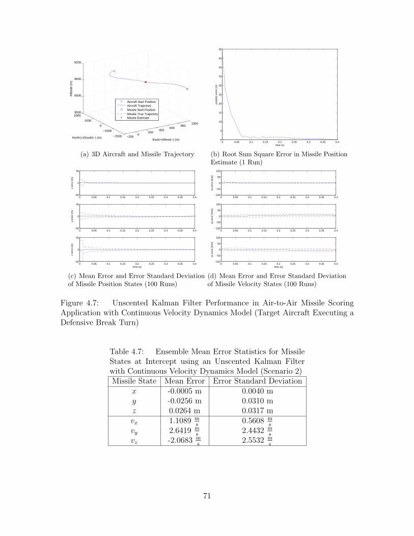
−2000

200400

600800

1000

−2000

−1000

0

1000

20003500

4000

4500

5000


Alti

tude

(m

)



0 0.05 0.1 0.15 0.2 0.25 0.3 0.35 0.40

5

10

15

20

25

30

35

40

45

50

posi

tion

erro

r (m

)

time (s)


0 0.05 0.1 0.15 0.2 0.25 0.3 0.35 0.4−50

0

50

x er

ror

(m)

0 0.05 0.1 0.15 0.2 0.25 0.3 0.35 0.4−50

0

50

y er

ror

(m)

0 0.05 0.1 0.15 0.2 0.25 0.3 0.35 0.4−50

0

50

z er

ror

(m)

time (s)


0 0.05 0.1 0.15 0.2 0.25 0.3 0.35 0.4−100

−50

0

50

100

vx e

rror

(m

/s)

0 0.05 0.1 0.15 0.2 0.25 0.3 0.35 0.4−100

−50

0

50

100

vy e

rror

(m

/s)

0 0.05 0.1 0.15 0.2 0.25 0.3 0.35 0.4−100

−50

0

50

100

vz e

rror

(m

/s)

time (s)


Figure 4.7: Unscented Kalman Filter Performance in Air-to-Air Missile ScoringApplication with Continuous Velocity Dynamics Model (Target Aircraft Executing aDefensive Break Turn)


x -0.0005 m 0.0040 my -0.0256 m 0.0310 mz 0.0264 m 0.0317 mvx 1.1089 m

s0.5608 m

s

vy 2.6419 ms

2.4432 ms

vz -2.0683 ms

2.5532 ms

71

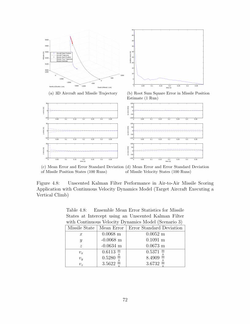
−1000

−500

0

500

1000

−3000

−2000

−1000

0

10005000

5100

5200

5300

5400

5500


Alti

tude

(m

)



0 0.05 0.1 0.15 0.2 0.25 0.3 0.350

5

10

15

20

25

30

35

40

45

50

posi

tion

erro

r (m

)

time (s)


0 0.05 0.1 0.15 0.2 0.25 0.3 0.35−50

0

50

x er

ror

(m)

0 0.05 0.1 0.15 0.2 0.25 0.3 0.35−50

0

50

y er

ror

(m)

0 0.05 0.1 0.15 0.2 0.25 0.3 0.35−50

0

50

z er

ror

(m)

time (s)


0 0.05 0.1 0.15 0.2 0.25 0.3 0.35−100

−50

0

50

100

vx e

rror

(m

/s)

0 0.05 0.1 0.15 0.2 0.25 0.3 0.35−100

−50

0

50

100

vy e

rror

(m

/s)

0 0.05 0.1 0.15 0.2 0.25 0.3 0.35−100

−50

0

50

100

vz e

rror

(m

/s)

time (s)


Figure 4.8: Unscented Kalman Filter Performance in Air-to-Air Missile ScoringApplication with Continuous Velocity Dynamics Model (Target Aircraft Executing aVertical Climb)


x 0.0068 m 0.0052 my -0.0068 m 0.1091 mz -0.0634 m 0.0673 mvx 0.6113 m

s0.5371 m

s

vy 0.5280 ms

8.4909 ms

vz 3.5622 ms

3.6732 ms

72

In all scenarios, the end-game mean position error is on the order of centimeters

with a worst-case standard deviation of 0.1265 meters. Furthermore, the range reso-

lution of the FMCW sensors is one of the primary limitations on position accuracy.

Since range accuracy is advertised as 2.5 percent of range, sensor range measurement

errors of 8.75 meters are expected at the scoring system’s maximum range.

The improvement in estimation of velocity states is not quite as dramatic, es-

pecially in axes with limited observability based on geometry. However, the plots

indicate that the error is constrained and the worst standard deviation at impact is

only 3.5622 meters per second or, equivalently, 6.924 nautical miles per hour.

4.8 Summary

This chapter began by outlining the methods for performing Monte Carlo sim-

ulations to assess the performance of the missile scoring system. Three drone flight

profiles were simulated to evaluate performance: non-maneuvering, 9G break-turn,

and vertical climb. The simulation truth data for the three scenarios was generated

using two 6DOF simulation software tools, Profgen and Argos 3.0. Next, this chap-

ter describes the procedure for filter tuning, a key aspect of improving Kalman filter

performance. The simulation methods were concluding by detailing the process for

generating random noise to simulate GRDCS target handoff, noise corrupted radar

measurements, and radar clutter.

The remainder of this chapter presented the results and analysis from the Monte

Carlo simulations. The CV dynamics model and the UKF algorithm were determined

to offer superior performance based on increased precision and reduced complexity.

Finally, the simulated performance of the UKF with CV dynamics model was pre-

sented for each of the three scenarios. The mean error and error standard deviation

was shown to be on the order of centimeters at impact. The next chapter further

evaluates the proposed air-to-air missile scoring system through flight testing.

73

V. Flight Test

The scoring system is evaluated through flight test by placing six automotive FMCW

sensors at fixed locations on the ground to simulate installation on an F-16 drone. A

series of passes in a Beechcraft C-12 aircraft are flown at low altitude over the sensor

array to simulate an inbound air-to-air missile. The configuration of the sensors

is adjusted between C-12 sorties to simulate different missile approach trajectories

towards the F-16 drone. The range and range-rate measurements from the sensors

are input into the UKF filter algorithm with a CV dynamics model to reconstruct the

3D position and velocity of the C-12 in a local ENU reference frame. The estimates

of the aircraft navigation parameters are compared with data generated by a GPS

system installed on the C-12. An error analysis is performed using the GPS data as

truth to assess the performance of the scoring system estimation.

In the remainder of this chapter, Section 5.1 provides a detailed description of

the scoring system implemented for testing. Section 5.2 contains a description of the

C-12 aircraft. Section 5.3 explains the sources of truth data for the flight testing.

Section 5.4 presents the flight profile flown to test the scoring system. Section 5.5

outlines the procedure for performing error analysis on the estimated aircraft position

and velocity. Section 5.6 describes the process for reducing sensor measurement bias

introduced by equipment limitations. Section 5.7 provides data on maximum sensor

detection range. Finally, Sections 5.8-5.10 compare simulation predictions with the

actual scoring system performance in reconstructing the trajectory of the C12 during

flight test.

5.1 Scoring System Description

Constructing the missile scoring system on the ground utilizes six COTS au-

tomotive FMCW sensors, two electronic control units (ECU), a laptop computer,

controller-area network (CAN) bus cables, a DC power supply, and three tower plat-

forms for mounting the sensors. The three towers are placed in a geometric configu-

ration to simulate the planform of the F-16 drone as illustrated in Figure 5.1. The

74

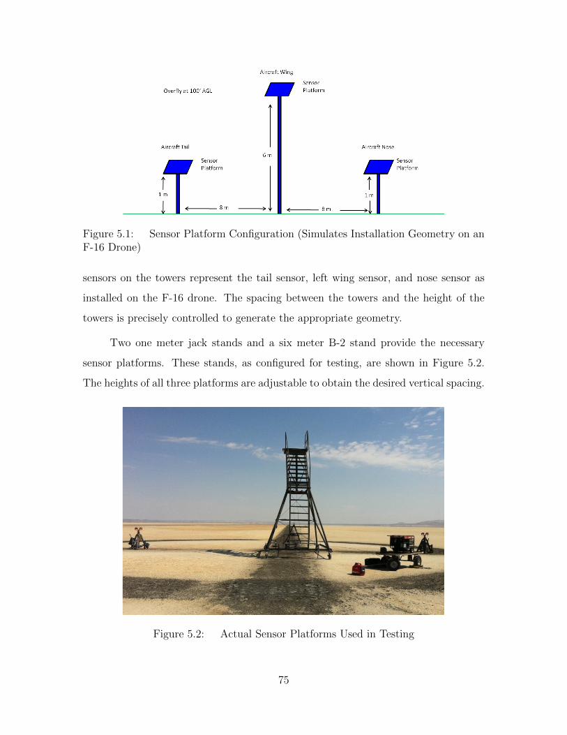
Figure 5.1: Sensor Platform Configuration (Simulates Installation Geometry on anF-16 Drone)

sensors on the towers represent the tail sensor, left wing sensor, and nose sensor as

installed on the F-16 drone. The spacing between the towers and the height of the

towers is precisely controlled to generate the appropriate geometry.

Two one meter jack stands and a six meter B-2 stand provide the necessary

sensor platforms. These stands, as configured for testing, are shown in Figure 5.2.

The heights of all three platforms are adjustable to obtain the desired vertical spacing.

Figure 5.2: Actual Sensor Platforms Used in Testing

75

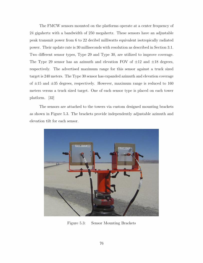
The FMCW sensors mounted on the platforms operate at a center frequency of

24 gigahertz with a bandwidth of 250 megahertz. These sensors have an adjustable

peak transmit power from 6 to 22 decibel milliwatts equivalent isotropically radiated

power. Their update rate is 30 milliseconds with resolution as described in Section 3.1.

Two different sensor types, Type 29 and Type 30, are utilized to improve coverage.

The Type 29 sensor has an azimuth and elevation FOV of ±12 and ±18 degrees,

respectively. The advertised maximum range for this sensor against a truck sized

target is 240 meters. The Type 30 sensor has expanded azimuth and elevation coverage

of ±15 and ±35 degrees, respectively. However, maximum range is reduced to 160

meters versus a truck sized target. One of each sensor type is placed on each tower

platform. [32]

The sensors are attached to the towers via custom designed mounting brackets

as shown in Figure 5.3. The brackets provide independently adjustable azimuth and

elevation tilt for each sensor.

Figure 5.3: Sensor Mounting Brackets

76

The ECUs and CAN bus cables are used to connect the six FMCW sensors

to the laptop computer for data output. Figure 5.4 depicts the electrical setup. As

shown in this figure, three sensors are connected to each ECU. The two ECUs connect

to the laptop computer via a dual channel CAN Personal Computer Memory Card

International Association (PCMCIA) Card. All equipment is powered by a diesel

generator through a 12 volt DC power supply. More detailed information on the

sensors and ECU is available in [32].

Figure 5.4: Sensor Electrical Wiring Setup

77

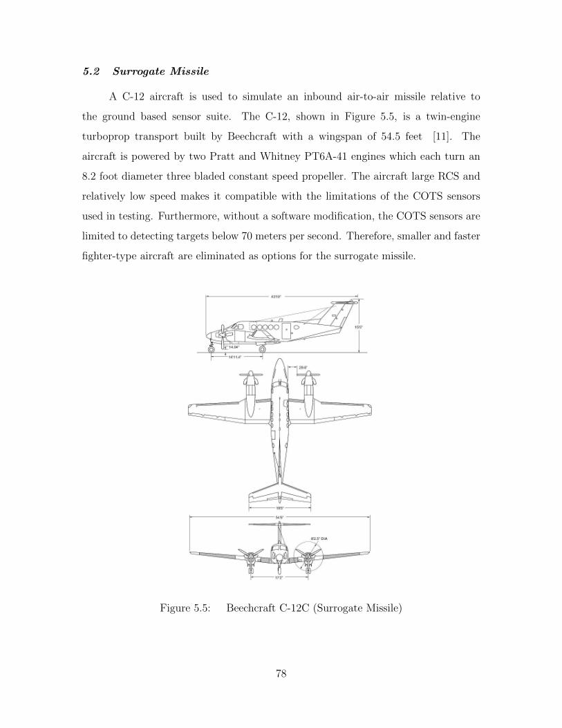
5.2 Surrogate Missile

A C-12 aircraft is used to simulate an inbound air-to-air missile relative to

the ground based sensor suite. The C-12, shown in Figure 5.5, is a twin-engine

turboprop transport built by Beechcraft with a wingspan of 54.5 feet [11]. The

aircraft is powered by two Pratt and Whitney PT6A-41 engines which each turn an

8.2 foot diameter three bladed constant speed propeller. The aircraft large RCS and

relatively low speed makes it compatible with the limitations of the COTS sensors

used in testing. Furthermore, without a software modification, the COTS sensors are

limited to detecting targets below 70 meters per second. Therefore, smaller and faster

fighter-type aircraft are eliminated as options for the surrogate missile.

Figure 5.5: Beechcraft C-12C (Surrogate Missile)

78

5.3 Truth Data

The Beechcraft C-12 used in testing is equipped with a GPS Aided Inertial

Navigation Reference (GAINR) Lite (GLite) system [2]. The GLite system records

real-time position measurements using a highly accurate blended GPS and inertial

measurement unit (IMU) navigation solution. The expected position and velocity

accuracy of the system is 1.5 feet and 0.02 feet per second, respectively. Data is

output at a rate of 50 hertz. The output from the GLite provides the C-12 truth data

for performing an error analysis.

The sensor ground locations are surveyed and marked by the National Geospa-

tial Intelligence-Agency to provide accuracy of 0.25 meters relative to WGS 84. There

are a total of nine surveyed sensor points as illustrated in Figure 5.6. Although, only

three sensor locations are used during any test flight, the additional survey locations

allow for the simulation of different missile approach azimuths towards the F-16 drone.

This is discussed further in Section 5.4.

N4

N3

N1

N2

T4

WT1

T2

T3

Tower Fly-ByLine

20° 45°

70°

Figure 5.6: Surveyed Sensor Locations

79

Additionally, all the surveyed points on the outer ring have an accuracy of 0.01 meters

relative to the center sensor reference location. A laser range finder is utilized to accu-

rately set the tower height for the desired sensor geometry. The surveyed coordinates

in conjunction with the laser range finder measurements provide the truth data for

the sensor locations.

The truth data for the C-12 and the sensor locations are defined in a local ENU

coordinate frame. The origin of the reference frame is defined at ground level under-

neath the center sensor. All error calculations are performed in this ENU reference

frame.

5.4 Test Execution

In order to simulate an inbound missile using the C-12, low-altitude flybys are

performed over the sensor array as shown in Figure 5.7. The flybys are executed at

100 feet above ground level (AGL) with a minimum altitude of 70 feet AGL for safety.

Since the center sensor platform is approximately 20 feet tall, the minimum altitude

provides 50 feet of clearance when flying over the tower.

Figure 5.7: C-12 Performing Low-Altitude Flyby Over Sensor Array

80

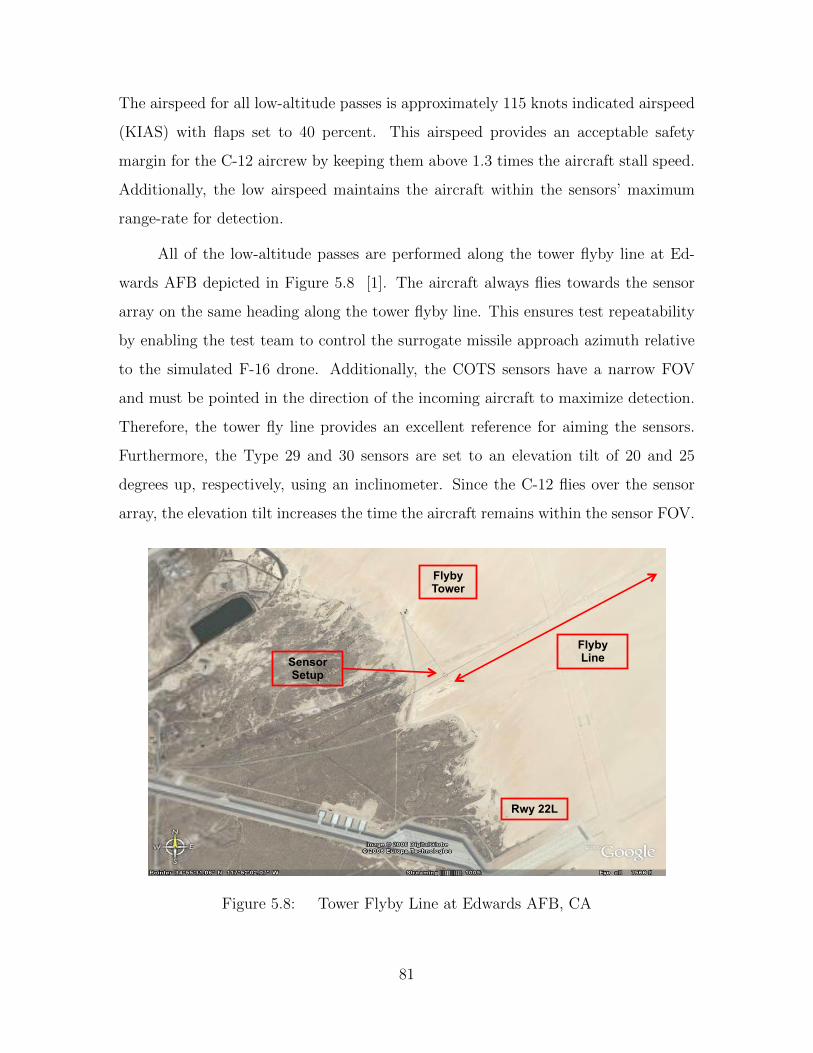
The airspeed for all low-altitude passes is approximately 115 knots indicated airspeed

(KIAS) with flaps set to 40 percent. This airspeed provides an acceptable safety

margin for the C-12 aircrew by keeping them above 1.3 times the aircraft stall speed.

Additionally, the low airspeed maintains the aircraft within the sensors’ maximum

range-rate for detection.

All of the low-altitude passes are performed along the tower flyby line at Ed-

wards AFB depicted in Figure 5.8 [1]. The aircraft always flies towards the sensor

array on the same heading along the tower flyby line. This ensures test repeatability

by enabling the test team to control the surrogate missile approach azimuth relative

to the simulated F-16 drone. Additionally, the COTS sensors have a narrow FOV

and must be pointed in the direction of the incoming aircraft to maximize detection.

Therefore, the tower fly line provides an excellent reference for aiming the sensors.

Furthermore, the Type 29 and 30 sensors are set to an elevation tilt of 20 and 25

degrees up, respectively, using an inclinometer. Since the C-12 flies over the sensor

array, the elevation tilt increases the time the aircraft remains within the sensor FOV.

Flyby Tower

Sensor Setup

Flyby Line

Rwy 22L

Figure 5.8: Tower Flyby Line at Edwards AFB, CA

81

In order to evaluate the system performance against different simulated missile

approach trajectories, the sensors are maneuvered to different positions on the ground.

Figure 5.6 illustrates the possible sensor locations. The left wing sensor is always

located at point W on the center tower. However, the nose and tail sensors are

adjusted between points N1-N4 and T1-T4, respectively. The location of the nose

and tail sensors must be consistent to replicate the geometry on the F-16 drone. For

example, if the nose sensor is placed at location N3, the tail sensor must be at location

T3. Since the surrogate missile always approaches the sensor array along the same

heading, adjusting the location of the nose and tail sensor effectively changes the

aspect angle of the F-16 drone as viewed from the approaching missile. When the

sensors are at positions N1, W, and T1 the drone aspect angle (AA) is 90 degrees. As

explained in Section 2.6, this geometry is most favorable for estimating the surrogate

missile navigation parameters because the angular spacing between the sensors relative

to the missile (C-12) is maximized. When the nose and tail sensors are rotated to the

remaining positions, F-16 drone aspect angles of 70, 45 and 20 degrees are simulated.

Each of these aspect angles represents progressively worse missile trajectories for

accurately estimating missile navigation parameters. The worst case geometry is a

missile approach path directly off the tail (0 degree AA) or nose (180 degrees AA) of

the F-16 drone.

Fifteen runs are performed at 90 and 45 degrees AA. Due to time constraints

and maintenance limitations, only one run is conducted at 70 degrees AA and five

runs are conducted at 20 degrees AA.

5.5 Error Calculations

An error analysis is performed by comparing the missile scoring software esti-

mates of the C-12 position and velocity with the GLite provided truth data. Since

simulations demonstrated the superior performance of the UKF with a CV dynamics

model, this is the only Kalman filter and dynamics model combination considered

82

during flight test. Figure 5.9 illustrates the general process for performing the error

analysis.

The UKF is initialized according to the process previously described in Sec-

tion 3.4. The inputs to the UKF include the fixed sensor locations and the time

stamped sensor measurements of range and range-rate. Based on this information,

the Kalman filter estimates the C-12 position and velocity in the local ENU coordinate

frame. Finally, this estimate is compared to GLite time space position information

(TSPI) to determine error.

The average position and velocity error is reporting by calculating the RSS error

for each run and then averaging across all runs at the same AA. The RSS position

error is calculated using

Perror =√

(xtest − xTSPI)2 + (ytest − yTSPI)2 + (ztest − zTSPI)2 (5.1)

The subscript test refers to the UKF estimates and the subscript TSPI specifies

GLite data.

Figure 5.9: Data Flow for Flight Test Error Analysis

83

Similarly, the RSS velocity error is determined from the equation

Verror =√

(vxtest − vxTSPI)2 + (vytest − vyTSPI

)2 + (vztest − vzTSPI)2 (5.2)

The position and velocity errors change with the decrease in slant range between

the surrogate missile and ground based sensors. Ideally, the UKF will continue to

reduce both position and velocity errors as the C-12 closes on the sensors since more

measurements are available to improve state estimation. Additionally, as the aircraft

closes on the sensor array, the changing sensor geometry relative to the C-12 will

impact the accuracy of state estimates. Therefore, the average RSS position and

velocity errors are reported within slant range bins. As detailed below in Section 5.7,

maximum sensor range demonstrated in testing against the C-12 is approximately 120

meters. Additionally, the are some runs where the sensors don’t detect the target until

inside of 100 meters. Therefore, slant range bins of 10 meters are selected starting with

100 meters. The error reporting bins are recorded in Table 5.1. The error calculated

at the center of each bin is reported for the entire bin. The Initial bin refers to the

error after the first measurement update is received. The Final bin specifies the error

after the last measurement update is received.

Table 5.1: Slant Range Bins for Error ReportingSlant Range Bins (m)

Initial> 90 - ≤ 100> 80 - ≤ 90> 70 - ≤ 80> 60 - ≤ 70> 50 - ≤ 60> 40 - ≤ 50

Final

84

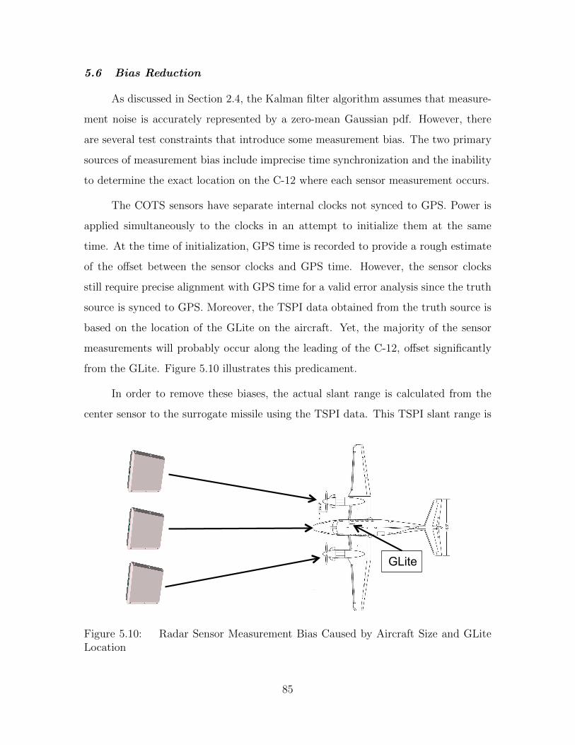
5.6 Bias Reduction

As discussed in Section 2.4, the Kalman filter algorithm assumes that measure-

ment noise is accurately represented by a zero-mean Gaussian pdf. However, there

are several test constraints that introduce some measurement bias. The two primary

sources of measurement bias include imprecise time synchronization and the inability

to determine the exact location on the C-12 where each sensor measurement occurs.

The COTS sensors have separate internal clocks not synced to GPS. Power is

applied simultaneously to the clocks in an attempt to initialize them at the same

time. At the time of initialization, GPS time is recorded to provide a rough estimate

of the offset between the sensor clocks and GPS time. However, the sensor clocks

still require precise alignment with GPS time for a valid error analysis since the truth

source is synced to GPS. Moreover, the TSPI data obtained from the truth source is

based on the location of the GLite on the aircraft. Yet, the majority of the sensor

measurements will probably occur along the leading of the C-12, offset significantly

from the GLite. Figure 5.10 illustrates this predicament.

In order to remove these biases, the actual slant range is calculated from the

center sensor to the surrogate missile using the TSPI data. This TSPI slant range is

GLite

Figure 5.10: Radar Sensor Measurement Bias Caused by Aircraft Size and GLiteLocation

85

then plotted versus time and overlaid with the radar slant range measurement from

the sensors on the center tower. A time shift is applied to visually align the TSPI

slant range with the observed slant range measurements from the sensors on the center

tower. This is done manually for each run and the resulting time shift is applied to

data from all sensors.

If all six sensor clocks are perfectly synchronized and all sensors take measure-

ments off the exact same location on the C-12, this technique completely removes

any measurement bias. However, in reality there may be some initial offset between

sensor clocks as well as different clock drift rates throughout the course of testing.

Furthermore, the size and shape of the C-12 will result in varied return locations.

5.7 Sensor Maximum Range

Based on the assumption that the RCS of a C-12 is similar to a truck, the

expected maximum detection range for the long range sensors is 240 meters. Nev-

ertheless, flight tests demonstrated a significantly shorter maximum detection range.

Table 5.2 records the average maximum detection range, standard deviation, and 95%

confidence interval for the test runs. For each run, the maximum detection range is

defined as the distance where all three long range sensors detect the target. The

reduced detection range will adversely impact the accuracy and precision of Kalman

filter state estimates since less observations are available to the filter.

Table 5.2: Maximum Range of COTS Frequency ModulatedContinuous Wave Radar Sensors Versus a C-12

Average Maximum Standard 95% Confidence Number ofDetection Range (m) Deviation (m) Interval (m) Samples

121.2 14.3 121.2± 4.9 35

5.8 Flight Test Predictions

Due to real-world test conditions, the analysis in Chapter IV is not directly ap-

plicable. Prior to flight testing, Monte Carlo simulations similar to those described in

86

Chapter IV are performed under conditions which better represent the flight test con-

ditions. In each simulation, the drone remains stationary and the missile approaches

the drone along a constant heading at an airspeed of 120 knots to replicate the C-12

profile. Furthermore, to accurately represent the flight test scenario, the missile ap-

proaches the drone from above and then misses the drone by 35 meters horizontally

as measured from the wingtip sensor. This simulates C-12 overflight of the sensor

array by 100 feet AGL. In addition, only the three sensors included in the flight test

are modeled in the simulation: nose, tail, and one wing. After completing the flight

tests, all simulations are adjusted to account for the shorter maximum sensor detec-

tion range discussed in Section 5.7. UKF initialization and generation of noisy sensor

measurements and false targets is performed according to the process outlined in Sec-

tion 4.4. To facilitate comparison between the flight test predictions and results, the

randomly generated initialization noise is saved and used in the flight test runs. As a

result, the simulations and flight tests start with the same initial error.

Four simulations of 30 Monte Carlo runs are performed to model each of the

different sensor configurations: 90, 70, 45, and 20 degrees AA. The RSS position and

velocity error of the UKF estimates are calculated and categorized into the slant range

bins discussed in Table 5.1. Additionally, the average RSS error and 95% confidence

interval is determined from the simulations. Executing 30 Monte Carlo runs ensures

the 95% confidence interval for the average RSS position error in the final slant range

bin converges to less than two meters. The results from the flight test predictions are

presented along with the flight test results in the next two sections.

5.9 C-12 Position Estimate Error

The flight test results presented in this section demonstrate that the proposed

missile scoring system successfully reduces error in estimates of the C-12 position. Al-

though the scoring performance is less than predicted through simulations, flight test

constraints are the probable culprit. This section identifies several factors associated

with flight test limitations contributing to the increased error.

87

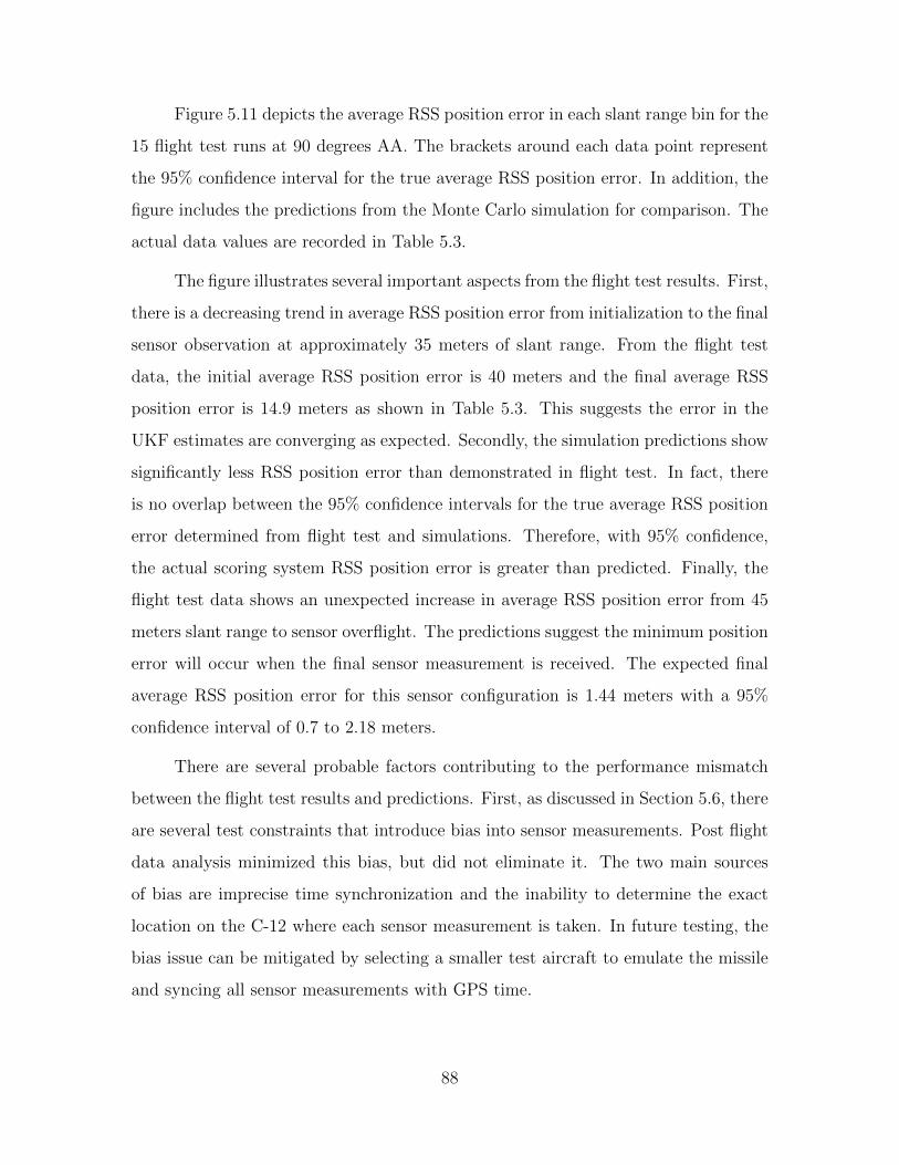
Figure 5.11 depicts the average RSS position error in each slant range bin for the

15 flight test runs at 90 degrees AA. The brackets around each data point represent

the 95% confidence interval for the true average RSS position error. In addition, the

figure includes the predictions from the Monte Carlo simulation for comparison. The

actual data values are recorded in Table 5.3.

The figure illustrates several important aspects from the flight test results. First,

there is a decreasing trend in average RSS position error from initialization to the final

sensor observation at approximately 35 meters of slant range. From the flight test

data, the initial average RSS position error is 40 meters and the final average RSS

position error is 14.9 meters as shown in Table 5.3. This suggests the error in the

UKF estimates are converging as expected. Secondly, the simulation predictions show

significantly less RSS position error than demonstrated in flight test. In fact, there

is no overlap between the 95% confidence intervals for the true average RSS position

error determined from flight test and simulations. Therefore, with 95% confidence,

the actual scoring system RSS position error is greater than predicted. Finally, the

flight test data shows an unexpected increase in average RSS position error from 45

meters slant range to sensor overflight. The predictions suggest the minimum position

error will occur when the final sensor measurement is received. The expected final

average RSS position error for this sensor configuration is 1.44 meters with a 95%

confidence interval of 0.7 to 2.18 meters.

There are several probable factors contributing to the performance mismatch

between the flight test results and predictions. First, as discussed in Section 5.6, there

are several test constraints that introduce bias into sensor measurements. Post flight

data analysis minimized this bias, but did not eliminate it. The two main sources

of bias are imprecise time synchronization and the inability to determine the exact

location on the C-12 where each sensor measurement is taken. In future testing, the

bias issue can be mitigated by selecting a smaller test aircraft to emulate the missile

and syncing all sensor measurements with GPS time.

88

Initial 95 85 75 65 55 45 Final0

10

20

30

40

50

60

70

Slant Range (m)

RS

S P

ositi

on E

rror

(m

)

Flight Test Result95% Confidence IntervalSimulation Prediction95% Confidence Interval

Figure 5.11: Comparison of Flight Test Results and Simulation Predictions for Av-erage Root Sum Square Error in Unscented Kalman Filter Estimates of C-12 Position(90◦ Drone Aspect Angle)

Table 5.3: C-12 Position Estimate Error per Slant Range Bin usingan Unscented Kalman Filter with Continuous Velocity Dynamics Model(90◦ Drone Aspect Angle)Range Bin (m) Average RSS Standard 95% Confidence

Position Error (m) Deviation (m) Interval (m)Initial 40.00 16.36 40.00± 9.06

> 90 - ≤ 100 39.81 22.82 39.81± 12.64> 80 - ≤ 90 33.45 22.85 33.45± 12.66> 70 - ≤ 80 26.30 19.41 26.30± 10.75> 60 - ≤ 70 20.63 15.78 20.63± 8.74> 50 - ≤ 60 16.41 13.04 16.41± 7.22> 40 - ≤ 50 12.31 10.72 12.31± 5.93

Final 14.90 10.30 14.90± 5.70

89

Secondly, in simulations the gating and data association algorithms described in

Section 3.3 demonstrated great effectiveness in eliminating false targets. In contrast,

numerous flight test runs show corruption in UKF estimates caused by false targets.

Figure 5.12 illustrates the issue with false targets. Initially, the UKF gates out all

measurements and shows a relatively constant RSS position error of approximately

0 0.5 1 1.5 2 2.50

20

40

60

80

100

120

Time (s)

RS

S P

ositi

on E

rror

(m

)

Large Error Increase

Flight Test ResultSimulation Prediction

(a) Predicted and Actual Root Sum Square Position Error

0 0.5 1 1.5 2 2.50

20

40

60

80

100

120

140

160

180

200

Time (s)

Sla

nt R

ange

(m

)

False RangeMeasurements

Wing Sensor (short range)Tail Sensor (short range)Tail Sensor (long range)Wing Sensor (long range)Nose Sensor (long range)Nose Sensor (short range)TSPI

(b) Radar Sensors Slant Range Measurements

Figure 5.12: Illustration of False Target Impact on Errors in Unscented KalmanFilter Position Estimates (Data from Run 11 at 90◦ Drone Aspect Angle)

90

30 meters. In Figure 5.12(a), from approximately 0.6 to 0.9 seconds the RSS position

error increases dramatically as the UKF updates the C-12 position estimate using

false sensor measurements. Figure 5.12(b) shows the raw range measurements from

the sensors. There is a significant grouping of false range measurements between 0

and 0.9 seconds.

The gating algorithm relies on the assumption that random false targets will

not exhibit both range and velocity comparable to the true target. However, the

false range measurements in Figure 5.12(b) are also associated with realistic sensor

speed measurements as shown in Figure 5.13. The probable source of these realistic

false targets is multipath off of the C-12 surfaces and propellor effects. Reducing the

gate size does not solve this issue because it eliminates the true target measurements

along with the false targets. Fortunately, the presence of such realistic false targets is

not anticipated during air-to-air missile scoring. Testing with a smaller target vehicle

would validate this assumption.

0 0.5 1 1.5 2 2.50

10

20

30

40

50

60

70

80

Time (s)

Vel

ocity

(m

/s)

False Range−rateMeasurements

Wing Sensor (short range)Tail Sensor (short range)Tail Sensor (long range)Wing Sensor (long range)Nose Sensor (long range)Nose Sensor (short range)

Figure 5.13: Illustration of False Target Speed Measurements (Data from Run 11at 90◦ Drone Aspect Angle)

91

Appendix B includes a comprehensive library of plots from all flight test runs.

There are four plots saved for each run. Two of the plots show the raw range and

speed measurements for all six sensors. The remaining two plots depict the calculated

RSS position and velocity error. These plots also include simulation predictions for

RSS position and velocity error for comparison.

Figure 5.14 illustrates the average RSS position error with the sensor config-

uration adjusted to represent a drone aspect angle of 45 degrees. This geometry is

less favorable for estimating C-12 navigation states because the angular spacing of

the sensors is reduced as viewed from the incoming aircraft. The simulations predict

a final RSS position error of 2.86 meters, compared to 1.44 meters when the sensors

are configured for 90 degrees AA. Once again the position errors determined during

flight testing are higher than the simulation predictions. There is no overlap between

the confidence intervals so the true average RSS position error of the flight tests are

higher than the prediction at 95% confidence .

The flight test data from 15 runs at 45 degrees AA are summarized in Table 5.4.

The average RSS position error is actually lower at 45 degrees AA than 90 degrees AA

in seven of the eight slant range bins. However, this is easily explained by the large

overlapping confidence intervals between the results at the two different aspect angles.

More runs are required to illustrate the improvement in state estimate accuracy based

on sensor geometry.

92

Initial 95 85 75 65 55 45 Final0

10

20

30

40

50

60

70

Slant Range (m)

RS

S P

ositi

on E

rror

(m

)



Table 5.4: C-12 Position Estimate Error per Slant Range Binusingan Unscented Kalman Filter with Continuous Velocity Dynamics Model(45◦ Drone Aspect Angle)Range Bin (m) Average RSS Standard 95% Confidence


> 90 - ≤ 100 27.79 22.44 27.79± 12.43> 80 - ≤ 90 24.26 18.25 24.26± 10.10> 70 - ≤ 80 21.76 15.36 21.76± 8.50> 60 - ≤ 70 20.31 13.44 20.31± 7.44> 50 - ≤ 60 15.92 11.18 15.921± 6.19> 40 - ≤ 50 10.93 9.13 10.93± 5.06

Final 20.60 8.51 20.60± 4.71

93

There is a substantial increase in average RSS position error between 45 meters

slant range and the final observation. This unexpected error increase is also present

in the test runs at 90 degrees AA. The large error increase is the result of noisier

measurements as the C-12 overflies the sensor array as shown in Figure 5.15.

0 0.5 1 1.5 2 2.50

20

40

60

80

100

120

140

160

180

200

Time (s)

Sla

nt R

ange

(m

)

Noisy RangeMeasurements


(a) Radar Sensors Slant Range Measurements

0 0.5 1 1.5 2 2.50

10

20

30

40

50

60

70

80

Time (s)

Vel

ocity

(m

/s)

Noisy Range−rateMeasurements


(b) Radar Sensors Speed Measurements

Figure 5.15: Illustration of Increase in Sensor Measurement Noise as C-12 Ap-proaches Sensor Overflight (Data from Run 1 at 45◦ Drone Aspect Angle)

94

As the C-12 approaches radar overflight, the aircraft presents greater planform

to the stationary ground sensors. The increased cross sectional area viewed by the

sensors results in numerous measurements off of widely varying parts of the aircraft.

In contrast, at greater distances the majority of the sensor measurements stem from

the leading edge of the aircraft.

Figure 5.16 depicts the results from four flight test runs executed with a sensor

geometry of 20 degrees AA. Due to the limited number of test runs, the average RSS

position error exhibits large 95% confidence intervals which partially overlap with the

predictions. The overall data trend is consistent with the previous runs at 90 and 45

degrees aspect angle. The data results are summarized in Table 5.5.

For completeness the simulation prediction and result from a single run per-

formed at 70 degrees aspect angle is included in Figure 5.17. Since the data is from

a single run, no confidence interval are presented.

Overall, the demonstrated performance of the system in estimating C-12 po-

sition is encouraging. Although the accuracy did not match simulation predictions,

there are substantial limitations present in the flight testing which will not exist in

the actual system. The limitations are primarily driven by cost and safety in exe-

cuting the flight test. Implementing the proposed system using customized FMCW

sensors designed for the missile scoring application will eliminate the bias present

due to absence of time syncing. Furthermore, sensors with a higher update rate and

better range resolution will further improve accuracy of position estimates. Finally,

the estimates of missile position improve significantly when the missile is flown to

impact with the drone due to advantageous alignment of the sensors relative to the

missile. This is confirmed by the difference between simulated system performance

in Chapter IV and flight test predictions. Chapter IV simulations demonstrated final

accuracy on the order of centimeters because the missile continued to impact. In

contrast, flight test predictions only anticipated accuracy on the order of meters since

the missile never got closer to the drone than approximately 30 meters.

95

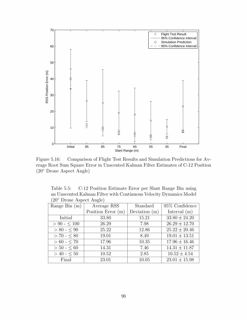
Initial 95 85 75 65 55 45 Final0

10

20

30

40

50

60

70

Slant Range (m)

RS

S P

ositi

on E

rror

(m

)



Table 5.5: C-12 Position Estimate Error per Slant Range Bin usingan Unscented Kalman Filter with Continuous Velocity Dynamics Model(20◦ Drone Aspect Angle)Range Bin (m) Average RSS Standard 95% Confidence


> 90 - ≤ 100 26.29 7.98 26.29± 12.70> 80 - ≤ 90 25.22 12.86 25.22± 20.46> 70 - ≤ 80 19.01 8.49 19.01± 13.51> 60 - ≤ 70 17.96 10.35 17.96± 16.46> 50 - ≤ 60 14.31 7.46 14.31± 11.87> 40 - ≤ 50 10.52 2.85 10.52± 4.54

Final 23.01 10.05 23.01± 15.98

96

Initial 95 85 75 65 55 45 Final0

10

20

30

40

50

60

70

Slant Range (m)

RS

S P

ositi

on E

rror

(m

)

Flight Test ResultSimulation Prediction95% Confidence Interval


5.10 C-12 Velocity Estimate Error

The flight test results in this section indicate the UKF software prevents the

velocity error from diverging, but overall RSS velocity error does not improve after

filter initialization. Figure 5.18 illustrates the predicted and actual average RSS ve-

locity error at 90 degrees AA. According to the predictions, the average RSS velocity

error will quickly converge to approximately three to six meters per second and then

remain constant as the missile tracks inbound to the target. However, flight testing

on the C-12 demonstrated an increase in average RSS velocity error after target ini-

tialization. The 95% confidence interval for the average RSS velocity error remains

relatively constant between 10 to 25 meters per second across the slant range bins.

Table 5.6 summarizes the data from the figure.

97

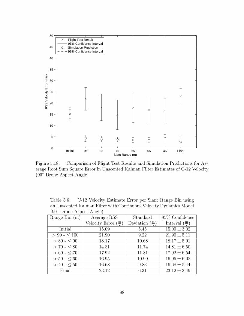
Initial 95 85 75 65 55 45 Final0

5

10

15

20

25

30

35

40

45

50

Slant Range (m)

RS

S V

eloc

ity E

rror

(m

/s)


Figure 5.18: Comparison of Flight Test Results and Simulation Predictions for Av-erage Root Sum Square Error in Unscented Kalman Filter Estimates of C-12 Velocity(90◦ Drone Aspect Angle)

Table 5.6: C-12 Velocity Estimate Error per Slant Range Bin usingan Unscented Kalman Filter with Continuous Velocity Dynamics Model(90◦ Drone Aspect Angle)Range Bin (m) Average RSS Standard 95% Confidence

Velocity Error (ms) Deviation (m

s) Interval (m

s)

Initial 15.09 5.45 15.09± 3.02> 90 - ≤ 100 21.90 9.22 21.90± 5.11> 80 - ≤ 90 18.17 10.68 18.17± 5.91> 70 - ≤ 80 14.81 11.74 14.81± 6.50> 60 - ≤ 70 17.92 11.81 17.92± 6.54> 50 - ≤ 60 16.95 10.99 16.95± 6.08> 40 - ≤ 50 16.68 9.83 16.68± 5.44

Final 23.12 6.31 23.12± 3.49

98

Since there is no overlap in the confidence intervals, the true average RSS ve-

locity error is greater than the prediction with 95% confidence. These results are

expected since the velocity state estimate error is highly correlated with the position

error. As illustrated in Section 2.7, velocity vector calculations from speed measure-

ments depend on knowledge of the sensor and target position. Therefore, since actual

RSS position errors presented in the previous section are greater than predicted it is

anticipated that velocity errors will also be higher. All of the factors driving the po-

sition error higher, such as measurement bias and inadequate gating of false targets,

also explains the higher velocity error.

Figure 5.19 and Table 5.7 record the velocity error when the sensor configura-

tion is changed to 45 degrees aspect angle. The errors are comparable to the runs

performed at 90 degrees aspect. Based on the large standard deviations and confi-

dence intervals for calculations of RSS velocity error, there are insufficient runs to

show the superior performance of the first sensor geometry.

The results in Figure 5.19 emphasis the significant increase in RSS velocity

error between 45 meters slant range and the final sensor measurement. As explained

in Section 5.9, this is the result of noisier measurements just prior to overflight based

on sensor LOS to C-12 planform.

Figures 5.20 and 5.21 and Table 5.8 show the results from the final two sensor

configurations of 20 and 70 degrees aspect angle. Due to the small number of runs

at 20 degrees AA, the standard deviation and 95% confidence interval for the RSS

velocity error is much larger than the previous geometries.

99

Initial 95 85 75 65 55 45 Final0

5

10

15

20

25

30

35

40

45

50

Slant Range (m)

RS

S V

eloc

ity E

rror

(m

/s)





s) Interval (m

s)

Initial 15.09 5.45 15.09± 3.02> 90 - ≤ 100 16.45 8.30 16.45± 4.59> 80 - ≤ 90 16.65 10.93 16.65± 6.05> 70 - ≤ 80 18.97 12.35 18.97± 6.84> 60 - ≤ 70 18.99 12.26 18.99± 6.79> 50 - ≤ 60 17.92 11.99 17.92± 6.64> 40 - ≤ 50 17.52 12.04 17.52± 6.67

Final 36.12 15.96 36.12± 8.84

100

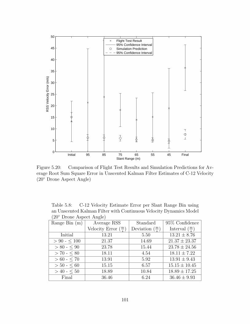
Initial 95 85 75 65 55 45 Final0

5

10

15

20

25

30

35

40

45

50

Slant Range (m)

RS

S V

eloc

ity E

rror

(m

/s)





s) Interval (m

s)

Initial 13.21 5.50 13.21± 8.76> 90 - ≤ 100 21.37 14.69 21.37± 23.37> 80 - ≤ 90 23.78 15.44 23.78± 24.56> 70 - ≤ 80 18.11 4.54 18.11± 7.22> 60 - ≤ 70 13.91 5.92 13.91± 9.43> 50 - ≤ 60 15.15 6.57 15.15± 10.45> 40 - ≤ 50 18.89 10.84 18.89± 17.25

Final 36.46 6.24 36.46± 9.93

101

Initial 95 85 75 65 55 45 Final0

5

10

15

20

25

30

35

40

45

50

Slant Range (m)

RS

S V

eloc

ity E

rror

(m

/s)

Flight Test ResultSimulation Prediction95% Confidence Interval


5.11 Summary

This chapter presented the methods, results, and analysis for conducting flight

testing on the proposed air-to-air missile scoring system. First, a detailed description

of the flight tested scoring system and C-12 surrogate missile was provided. Secondly,

the source of truth data for the sensor positions and the surrogate missile position

and velocity was described. Next, the test execution procedures were explained to

repeatably produce the desired trajectory. Additionally, this chapter described the

process for calculating position and velocity error to include removal of sensor mea-

surement bias. Finally, the test results were presented and analyzed to include average

maximum sensor range and missile estimate RSS position and velocity error at each

drone aspect angle. The successful implementation of the air-to-air scoring system

demonstrates the potential for future application in flight test and evaluation. The

102

next and final chapter of this research provides a summary of relevant results and

proposes future research for missile scoring.

103

VI. Conclusions and Recommendations

This research demonstrated the potential for a low-cost, short-range, radar based air-

to-air missile scoring system for installation on drone aircraft. The system presented

utilized seven FMCW radar sensors strategically placed on the drone to provide 360

degrees spherical coverage around the aircraft. The sensors measure range and range-

rate to the missile in-flight out to a distance of approximately 350 meters. A Kalman

filter software algorithm fuses the sensor measurements with a missile dynamics model

to estimate kinematic parameters of the missile in flight. Basic gating and data

association was implemented in the software algorithm to deal with potential radar

clutter. Missile position and velocity were the key parameters of interest in missile

flight path reconstruction.

6.1 Summary of Results

Based on the scoring strategy pursued in this research, the optimal drone config-

uration consists of placing sensors on the nose, tail, and both wing tips of the aircraft.

In order to minimize aircraft masking, radar sensor locations were selected on both

the upper and lower surface of the nose and wing tips such that four sensors maintain

LOS to a missile approaching from above or below the aircraft. Since the scoring

system relies on the concept of trilateration, the most accurate estimates of missile

kinematic parameters require sensor placement to maximize angular separation as

viewed from the incoming missile.

This research evaluated three missile dynamics model for Kalman filter imple-

mentation: constant velocity, constant acceleration, and 3D coordinated turn. The

comparison was conducted by performing 100-run Monte Carlo simulations using three

realistic missile trajectory scenarios. The constant dynamics model demonstrated

greater precision in estimating missile position and velocity at impact. Additionally,

the constant velocity dynamics model is simpler and computationally cheaper, since

it only tracks missile position and velocity, while the other dynamics models also

estimate missile acceleration.

104

This research also compared the performance of three popular nonlinear Kalman

filters for this missile scoring application: an extended Kalman filter, unscented

Kalman filter, and particle filter. Once again, the evaluation was conducted by exe-

cuting three 100 run Monte Carlo simulations. The unscented Kalman filter demon-

strated a clear advantage in precision of missile position and velocity states at impact.

Furthermore, the extended Kalman filter required cumbersome calculations of numer-

ous partial derivatives for implementation. The particle filter suffered from extreme

vulnerability to particle starvation. Overcoming this limitation required large par-

ticle numbers and constant resampling which grossly increased computer processing

requirements. Based on these simulation results, the unscented Kalman filter was the

best choice for this air-to-air missile scoring application.

Simulation results from three scenarios demonstrated overall position accuracy

and precision of the proposed scoring system on the order of centimeters. The sim-

ulated scenarios included a drone flying straight and level, executing a high-g break

turn, and performing an aggressive vertical climb. Over the three scenarios, the

greatest error in a position state estimate at impact by the unscented Kalman filter

with a continuous velocity dynamics model was just 6.34 centimeters. Similarly, the

worst-case precision at impact was characterized by a standard deviation of 12.65

centimeters. Furthermore, results were based on commercially available automotive

sensors not optimized for this application. Improvement in sensor range resolution

offers one method for further improving end-game position accuracy and precision.

Simulation results showed slightly greater error in estimating missile velocity at

impact. Using an unscented Kalman filter with continuous velocity dynamics model,

the worst-case mean error in any of the velocity states at impact was 3.5622 meters

per second. Additionally, the greatest standard deviation in any velocity state was

8.4909 meters per second. Velocity estimation also suffered from observability issues,

since sensors could only measure range-rate along their LOS to the missile. Therefore,

the worst precision in velocity estimation occurred in the velocity components nearly

105

orthogonal to all sensors’ LOS with the incoming missile. Despite these limitations,

the velocity errors at impact were small relative to the speed the of a missile.

Flight testing presented in this research supports the feasibility of employing

this air-to-air missile scoring system. Using commercially available equipment, the

proposed drone sensor configuration was reconstructed on the ground. A C-12 aircraft

was flown at low-altitude over the sensor array to simulate a missile missing the

target. Using the sensor measurements of the C-12 during overflight, the Kalman filter

software successfully reconstructed the missile trajectory, reducing root sum square

position error from initialization to overflight. Although error in position estimates

were worse than predicted in simulations, the data suggests flight test limitations and

not scoring system shortfalls were the primary cause of the reduction in performance.

The inability to sync sensor measurements with GPS time and the large size of the

surrogate missile (i.e., C-12) introduced significant bias into sensor measurements.

Additionally, raw sensor data showed unrealistic false targets in the immediate vicinity

of the C-12, probably caused by multipath or propeller effects. The software gating

algorithms were only partially effective in eliminating this clutter due to its proximity

to the real target.

6.2 Future Work

There are several areas in which additional research has the potential to signifi-

cantly improve the usefulness of the system. First, software or hardware adjustments

which improve the accuracy and/or precision of the system estimates are worth ex-

ploring. Secondly, follow on research should increase the autonomy of the system by

removing the scoring system’s dependence on an external system for target initial-

izaiton. Finally, additional flight testing is necessary to verify system performance.

The remainder of this chapter will explore each of these in greater detail.

The proposed missile scoring system is intended for missile test and evalua-

tion; therefore, there is no requirement for real-time reconstruction of the missile

trajectory. As a result, the Kalman filter software algorithm may be adjusted to

106

incorporate smoothing techniques. When reconstructing the missile trajectory dur-

ing post-mission processing, all sensor measurements during the missile intercept are

available to the Kalman filter. A Kalman filter smoother takes advantage of this

knowledge when performing state estimation. At any given time in the missile tra-

jectory, the Kalman filter smoother determines an optimal estimate of the missile

position and velocity based on past and future measurements. The ability to con-

sider future measurements allows the Kalman filter to improve estimate precision and

accuracy. There are several different algorithms available for performing smoothing.

Maybeck provides an in-depth discussion on the topic of Kalman filter smoothing [19].

Incorporating variable filter tuning in the Kalman filter algorithm is another

option to improve system performance. As discussed in Section 4.3, two key filter

tuning parameters include the dynamics noise strength, Q, and the observation noise

strength matrix, R. The ratio of these two matrices tells the Kalman filter how much

to weight the missile dynamics model versus the sensor measurements. However, the

range resolution of the commercial sensors used in this research are specified as a

percentage of slant range to the target. Therefore, the sensors provide more accurate

measurements as the missile gets closer to the drone. Intuitively, this suggests the best

estimate of missile kinematics will occur if the Q-to-R ratio is varied according to the

distance from the drone aircraft. Additional research in this area should experiment

with different methods for adjusting the Q-to-R ratio and characterize the degree of

performance improvement.

The sensor specifications necessary to achieve a desired scoring performance is

not directly addressed in this research. The automotive FMCW sensors considered in

this research are not adequate for actual implementation for several different reasons.

First, they lack the required sensitivity to detect a small RCS target like a missile,

especially at a range of 350 meters. Secondly, the speed of a missile is outside their

capability for range-rate measurements. Thirdly, the sensors have a narrow FOV

and would not provide spherical coverage around a drone aircraft. Finally, their slow

update rate and inability to sync to a GPS clock is undesirable for this application. So

107

presumably, implementation of this scoring system requires some careful consideration

as to the design of an appropriate sensor. Future research could characterize the

precision and accuracy in state estimation provided by different sensor resolutions

and update rates. This knowledge would enable a customer to select or design a

sensor with the minimum required specifications for the missile scoring application.

This is critical to reduce cost since these sensors will be destroyed along with the

drone aircraft during missile testing.

One limitation of the proposed system is the reliance on an external initial-

ization system such as the GRDCS. With the current software, the scoring system

requires this aide. Fortunately, the GRDCS is a range safety system so high relia-

bility is expected. However, with adjustments to the missile scoring software it is

possible to initialize the target solely using sensor measurements. As discussed in

Section 2.6, simultaneous observations from four sensors provide enough information

to uniquely identify the 3D position of the missile. However, the challenge stems

from the possibility of false measurements. If four sensors simultaneously receive

three range measurements for possible targets, the actual number of potential targets

formed using multilateration is 43 or 64. Therefore, in the presence of radar clutter,

the software scoring algorithm must include some form of track scoring or hypothesis

testing [5] and [4]. In track scoring each potential target is identified as a track and

additional measurements compatible with the track increase the track score. Even-

tually with sufficient updates the track transitions into a target. In contrast, tracks

that do not receive reasonable sensor updates are discarded as clutter. Obviously, in

a high clutter environment, the number of tracks can increase rapidly becoming com-

putationally burdensome. Fortunately, limited clutter is anticipated in this end-game

missile scoring application; therefore, false sensor measurements are expected rarely.

Nevertheless, significant changes to the missile scoring system software are required

to enable autonomous target initialization.

An additional benefit of modifying the software to incorporate track scoring is

the expansion into the realm of scoring multiple missiles. There are numerous possible

108

scenarios in which testers may desire to evaluate multiple missile launches against a

single target. Track scoring is one method to allow for multiple targets without any

modifications to the scoring system hardware.

Lastly, further work on the proposed air-to-air scoring system should include

additional flight testing to verify anticipated performance. The flight testing executed

as part of this research demonstrated proof-of-concept, but test limitations prevented

verification of actual system performance. Future flight testing should address the

GPS syncing of sensors and modify the sensor firmware to allow for a higher speed

target more representative of a missile. Removal of the target speed restrictions would

also enable testing to proceed with a fighter-sized target as the surrogate missile

thereby minimizing issues with multipath and reducing bias in sensor measurements.

6.3 Summary

In summary, this research successfully designed, implemented, and compared

several estimation techniques for air-to-air missile vector scoring. Exhaustive sim-

ulations were performed, and actual flight tests were executed. While comparison

between simulations and flight tests showed some discrepancies, this research shows

promise for actual implementation with modifications and opens the door to exciting

follow-on work.

109

Appendix A. Simulation Results

A.1 Extended Kalman Filter Simulations

−1500−1000

−5000

5001000

1500

0

500

1000

1500

2000

2500

30000

1000

2000

3000

4000

5000


Alti

tude

(m

)



0 0.05 0.1 0.15 0.2 0.25 0.3 0.35 0.4 0.450

5

10

15

20

25

30

35

40

45

50

posi

tion

erro

r (m

)

time (s)


0 0.05 0.1 0.15 0.2 0.25 0.3 0.35 0.4 0.45−50

0

50

x er

ror

(m)

0 0.05 0.1 0.15 0.2 0.25 0.3 0.35 0.4 0.45−50

0

50

y er

ror

(m)

0 0.05 0.1 0.15 0.2 0.25 0.3 0.35 0.4 0.45−50

0

50

z er

ror

(m)

time (s)


0 0.05 0.1 0.15 0.2 0.25 0.3 0.35 0.4 0.45−40

−20

0

20

40

vx e

rror

(m

/s)

0 0.05 0.1 0.15 0.2 0.25 0.3 0.35 0.4 0.45−40

−20

0

20

40

vy e

rror

(m

/s)

0 0.05 0.1 0.15 0.2 0.25 0.3 0.35 0.4 0.45−40

−20

0

20

40

vz e

rror

(m

/s)

time (s)


Figure A.1: Extended Kalman Filter Performance in Air-to-Air Missile Scor-ing Application with Continuous Velocity Dynamics Model (Target Aircraft Non-maneuvering)

110

−1500−1000

−5000

5001000

1500

0

500

1000

1500

2000

2500

30000

1000

2000

3000

4000

5000


Alti

tude

(m

)



0 0.05 0.1 0.15 0.2 0.25 0.3 0.35 0.4 0.450

5

10

15

20

25

30

35

40

45

50

posi

tion

erro

r (m

)time (s)


0 0.05 0.1 0.15 0.2 0.25 0.3 0.35 0.4 0.45−50

0

50

x er

ror

(m)

0 0.05 0.1 0.15 0.2 0.25 0.3 0.35 0.4 0.45−50

0

50

y er

ror

(m)

0 0.05 0.1 0.15 0.2 0.25 0.3 0.35 0.4 0.45−50

0

50

z er

ror

(m)

time (s)


0 0.05 0.1 0.15 0.2 0.25 0.3 0.35 0.4 0.45−40

−20

0

20

40

vx e

rror

(m

/s)

0 0.05 0.1 0.15 0.2 0.25 0.3 0.35 0.4 0.45−40

−20

0

20

40

vy e

rror

(m

/s)

0 0.05 0.1 0.15 0.2 0.25 0.3 0.35 0.4 0.45−40

−20

0

20

40

vz e

rror

(m

/s)

time (s)


Figure A.2: Extended Kalman Filter Performance in Air-to-Air Missile ScoringApplication with Continuous Acceleration Dynamics Model (Target Aircraft Non-maneuvering)

111

−1500−1000

−5000

5001000

1500

0

500

1000

1500

2000

2500

30000

1000

2000

3000

4000

5000


Alti

tude

(m

)



0 0.05 0.1 0.15 0.2 0.25 0.3 0.35 0.4 0.450

5

10

15

20

25

30

35

40

45

50

posi

tion

erro

r (m

)time (s)


0 0.05 0.1 0.15 0.2 0.25 0.3 0.35 0.4 0.45−50

0

50

x er

ror

(m)

0 0.05 0.1 0.15 0.2 0.25 0.3 0.35 0.4 0.45−50

0

50

y er

ror

(m)

0 0.05 0.1 0.15 0.2 0.25 0.3 0.35 0.4 0.45−50

0

50

z er

ror

(m)

time (s)


0 0.05 0.1 0.15 0.2 0.25 0.3 0.35 0.4 0.45−40

−20

0

20

40

vx e

rror

(m

/s)

0 0.05 0.1 0.15 0.2 0.25 0.3 0.35 0.4 0.45−40

−20

0

20

40

vy e

rror

(m

/s)

0 0.05 0.1 0.15 0.2 0.25 0.3 0.35 0.4 0.45−40

−20

0

20

40

vz e

rror

(m

/s)

time (s)


Figure A.3: Extended Kalman Filter Performance in Air-to-Air Missile Scor-ing Application with 3D Coordinated Turn Dynamics Model (Target Aircraft Non-maneuvering)

112

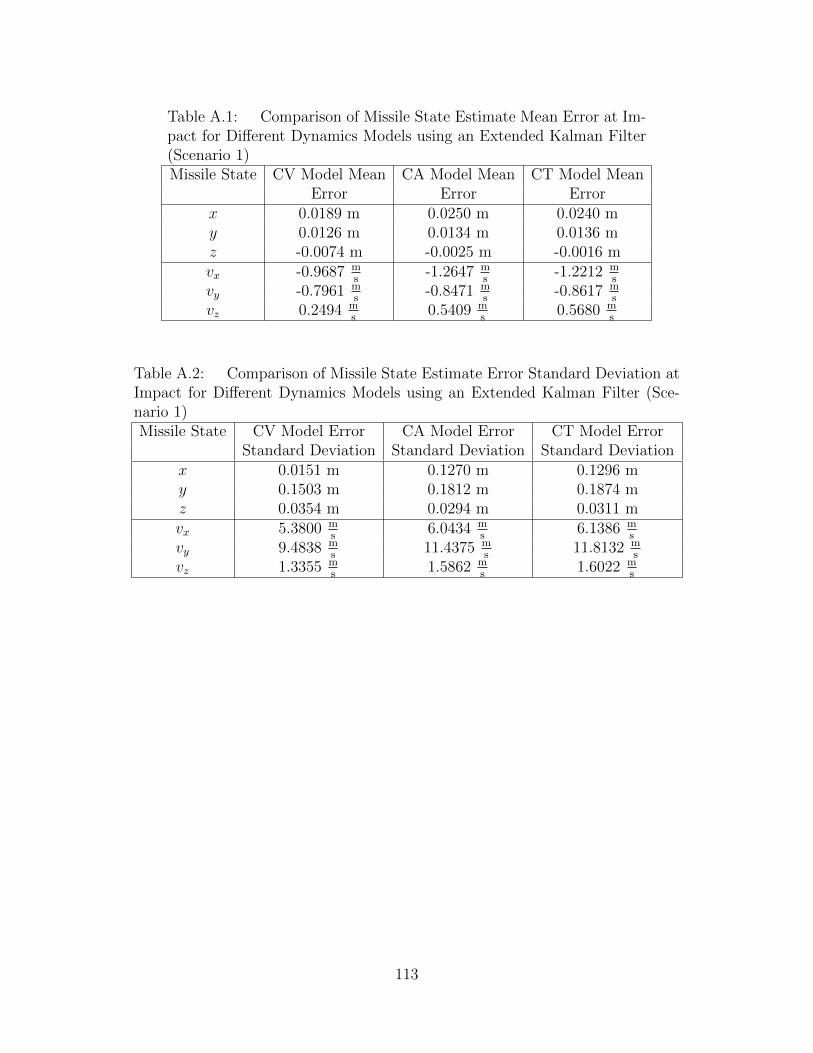
Table A.1: Comparison of Missile State Estimate Mean Error at Im-pact for Different Dynamics Models using an Extended Kalman Filter(Scenario 1)Missile State CV Model Mean CA Model Mean CT Model Mean

Error Error Errorx 0.0189 m 0.0250 m 0.0240 my 0.0126 m 0.0134 m 0.0136 mz -0.0074 m -0.0025 m -0.0016 mvx -0.9687 m

s-1.2647 m

s-1.2212 m

s

vy -0.7961 ms

-0.8471 ms

-0.8617 ms

vz 0.2494 ms

0.5409 ms

0.5680 ms

Table A.2: Comparison of Missile State Estimate Error Standard Deviation atImpact for Different Dynamics Models using an Extended Kalman Filter (Sce-nario 1)Missile State CV Model Error CA Model Error CT Model Error


s6.0434 m

s6.1386 m

s

vy 9.4838 ms

11.4375 ms

11.8132 ms

vz 1.3355 ms

1.5862 ms

1.6022 ms

113

−2000

200400

600800

1000

−2000

−1000

0

1000

20003500

4000

4500

5000


Alti

tude

(m

)



0 0.05 0.1 0.15 0.2 0.25 0.3 0.35 0.40

5

10

15

20

25

30

35

40

45

50

posi

tion

erro

r (m

)

time (s)


0 0.05 0.1 0.15 0.2 0.25 0.3 0.35 0.4−50

0

50

x er

ror

(m)

0 0.05 0.1 0.15 0.2 0.25 0.3 0.35 0.4−50

0

50

y er

ror

(m)

0 0.05 0.1 0.15 0.2 0.25 0.3 0.35 0.4−50

0

50

z er

ror

(m)

time (s)


0 0.05 0.1 0.15 0.2 0.25 0.3 0.35 0.4−100

−50

0

50

100

vx e

rror

(m

/s)

0 0.05 0.1 0.15 0.2 0.25 0.3 0.35 0.4−100

−50

0

50

100

vy e

rror

(m

/s)

0 0.05 0.1 0.15 0.2 0.25 0.3 0.35 0.4−100

−50

0

50

100

vz e

rror

(m

/s)

time (s)


Figure A.4: Extended Kalman Filter Performance in Air-to-Air Missile ScoringApplication with Continuous Velocity Dynamics Model (Target Aircraft Executing aDefensive Break Turn)

114

−2000

200400

600800

1000

−2000

−1000

0

1000

20003500

4000

4500

5000


Alti

tude

(m

)



0 0.05 0.1 0.15 0.2 0.25 0.3 0.35 0.40

5

10

15

20

25

30

35

40

45

50

posi

tion

erro

r (m

)time (s)


0 0.05 0.1 0.15 0.2 0.25 0.3 0.35 0.4−50

0

50

x er

ror

(m)

0 0.05 0.1 0.15 0.2 0.25 0.3 0.35 0.4−50

0

50

y er

ror

(m)

0 0.05 0.1 0.15 0.2 0.25 0.3 0.35 0.4−50

0

50

z er

ror

(m)

time (s)


0 0.05 0.1 0.15 0.2 0.25 0.3 0.35 0.4−100

−50

0

50

100

vx e

rror

(m

/s)

0 0.05 0.1 0.15 0.2 0.25 0.3 0.35 0.4−100

−50

0

50

100

vy e

rror

(m

/s)

0 0.05 0.1 0.15 0.2 0.25 0.3 0.35 0.4−100

−50

0

50

100

vz e

rror

(m

/s)

time (s)


Figure A.5: Extended Kalman Filter Performance in Air-to-Air Missile Scoring Ap-plication with Continuous Acceleration Dynamics Model (Target Aircraft Executinga Defensive Break Turn)

115

−2000

200400

600800

1000

−2000

−1000

0

1000

20003500

4000

4500

5000


Alti

tude

(m

)



0 0.05 0.1 0.15 0.2 0.25 0.3 0.35 0.40

5

10

15

20

25

30

35

40

45

50

posi

tion

erro

r (m

)time (s)


0 0.05 0.1 0.15 0.2 0.25 0.3 0.35 0.4−50

0

50

x er

ror

(m)

0 0.05 0.1 0.15 0.2 0.25 0.3 0.35 0.4−50

0

50

y er

ror

(m)

0 0.05 0.1 0.15 0.2 0.25 0.3 0.35 0.4−50

0

50

z er

ror

(m)

time (s)


0 0.05 0.1 0.15 0.2 0.25 0.3 0.35 0.4−100

−50

0

50

100

vx e

rror

(m

/s)

0 0.05 0.1 0.15 0.2 0.25 0.3 0.35 0.4−100

−50

0

50

100

vy e

rror

(m

/s)

0 0.05 0.1 0.15 0.2 0.25 0.3 0.35 0.4−100

−50

0

50

100

vz e

rror

(m

/s)

time (s)


Figure A.6: Extended Kalman Filter Performance in Air-to-Air Missile ScoringApplication with 3D Coordinated Turn Dynamics Model (Target Aircraft Executinga Defensive Break Turn)

116


Error Error Errorx 0.0034 m 0.0000 m -0.0012 my -0.0199 m -0.0153 m -0.0120 mz 0.0256 m 0.0250 m 0.0186 mvx 0.9924 m

s0.6511 m

s0.7266 m

s

vy 2.2057 ms

1.9207 ms

1.2400 ms

vz -1.9546 ms

-2.4550 ms

-1.2838 ms



s1.9879 m

s2.3412 m

s

vy 6.2837 ms

12.9057 ms

9.1882 ms

vz 8.5262 ms

19.7077 ms

12.0386 ms

117

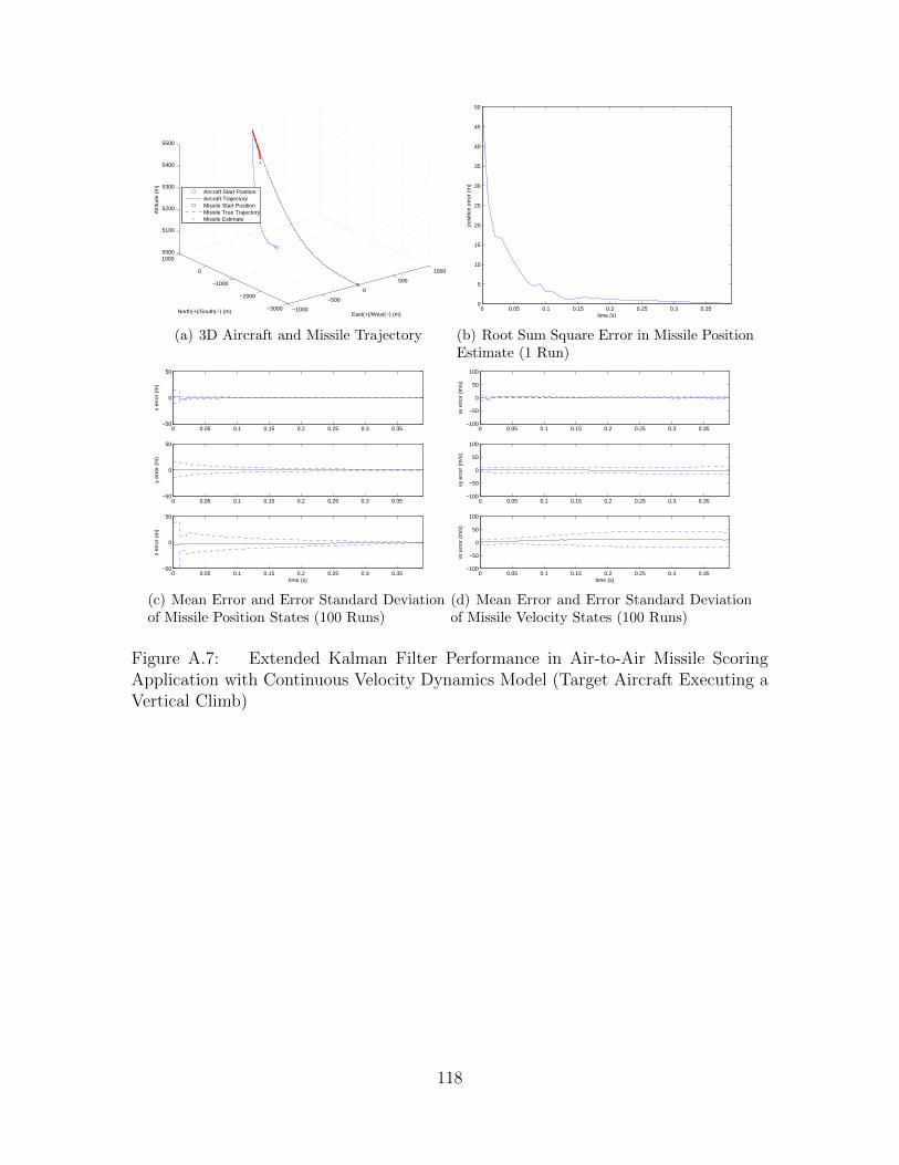
−1000

−500

0

500

1000

−3000

−2000

−1000

0

10005000

5100

5200

5300

5400

5500


Alti

tude

(m

)



0 0.05 0.1 0.15 0.2 0.25 0.3 0.350

5

10

15

20

25

30

35

40

45

50

posi

tion

erro

r (m

)

time (s)


0 0.05 0.1 0.15 0.2 0.25 0.3 0.35−50

0

50

x er

ror

(m)

0 0.05 0.1 0.15 0.2 0.25 0.3 0.35−50

0

50

y er

ror

(m)

0 0.05 0.1 0.15 0.2 0.25 0.3 0.35−50

0

50

z er

ror

(m)

time (s)


0 0.05 0.1 0.15 0.2 0.25 0.3 0.35−100

−50

0

50

100

vx e

rror

(m

/s)

0 0.05 0.1 0.15 0.2 0.25 0.3 0.35−100

−50

0

50

100

vy e

rror

(m

/s)

0 0.05 0.1 0.15 0.2 0.25 0.3 0.35−100

−50

0

50

100

vz e

rror

(m

/s)

time (s)


Figure A.7: Extended Kalman Filter Performance in Air-to-Air Missile ScoringApplication with Continuous Velocity Dynamics Model (Target Aircraft Executing aVertical Climb)

118

−1000

−500

0

500

1000

−3000

−2000

−1000

0

10005000

5100

5200

5300

5400

5500


Alti

tude

(m

)



0 0.05 0.1 0.15 0.2 0.25 0.3 0.350

5

10

15

20

25

30

35

40

45

50

posi

tion

erro

r (m

)time (s)


0 0.05 0.1 0.15 0.2 0.25 0.3 0.35−50

0

50

x er

ror

(m)

0 0.05 0.1 0.15 0.2 0.25 0.3 0.35−50

0

50

y er

ror

(m)

0 0.05 0.1 0.15 0.2 0.25 0.3 0.35−50

0

50

z er

ror

(m)

time (s)


0 0.05 0.1 0.15 0.2 0.25 0.3 0.35−100

−50

0

50

100

vx e

rror

(m

/s)

0 0.05 0.1 0.15 0.2 0.25 0.3 0.35−100

−50

0

50

100

vy e

rror

(m

/s)

0 0.05 0.1 0.15 0.2 0.25 0.3 0.35−100

−50

0

50

100

vz e

rror

(m

/s)

time (s)


Figure A.8: Extended Kalman Filter Performance in Air-to-Air Missile Scoring Ap-plication with Continuous Acceleration Dynamics Model (Target Aircraft Executinga Vertical Climb)

119

−1000

−500

0

500

1000

−3000

−2000

−1000

0

10005000

5100

5200

5300

5400

5500


Alti

tude

(m

)



0 0.05 0.1 0.15 0.2 0.25 0.3 0.350

5

10

15

20

25

30

35

40

45

50

posi

tion

erro

r (m

)time (s)


0 0.05 0.1 0.15 0.2 0.25 0.3 0.35−50

0

50

x er

ror

(m)

0 0.05 0.1 0.15 0.2 0.25 0.3 0.35−50

0

50

y er

ror

(m)

0 0.05 0.1 0.15 0.2 0.25 0.3 0.35−50

0

50

z er

ror

(m)

time (s)


0 0.05 0.1 0.15 0.2 0.25 0.3 0.35−100

−50

0

50

100

vx e

rror

(m

/s)

0 0.05 0.1 0.15 0.2 0.25 0.3 0.35−100

−50

0

50

100

vy e

rror

(m

/s)

0 0.05 0.1 0.15 0.2 0.25 0.3 0.35−100

−50

0

50

100

vz e

rror

(m

/s)

time (s)


Figure A.9: Extended Kalman Filter Performance in Air-to-Air Missile ScoringApplication with 3D Coordinated Turn Dynamics Model (Target Aircraft Executinga Vertical Climb)

120


Error Error Errorx 0.0088 m -0.0017 m -0.0026 my 0.0050 m 0.0219 m 0.0226 mz -0.0724 m -0.0793 m -0.0787 mvx 0.7081 m

s0.0991 m

s0.0299 m

s

vy -0.3869 ms

-1.7269 ms

-1.7766 ms

vz 3.9596 ms

4.6376 ms

4.6444 ms



s2.1058 m

s2.1245 m

s

vy 11.8460 ms

15.1679 ms

15.1300 ms

vz 13.7464 ms

26.2245 ms

26.2736 ms

121

A.2 Unscented Kalman Filter Simulations

−1500−1000

−5000

5001000

1500

0

500

1000

1500

2000

2500

30000

1000

2000

3000

4000

5000


Alti

tude

(m

)



0 0.05 0.1 0.15 0.2 0.25 0.3 0.35 0.4 0.450

5

10

15

20

25

30

35

40

45

50

posi

tion

erro

r (m

)

time (s)


0 0.05 0.1 0.15 0.2 0.25 0.3 0.35 0.4 0.45−50

0

50

x er

ror

(m)

0 0.05 0.1 0.15 0.2 0.25 0.3 0.35 0.4 0.45−50

0

50

y er

ror

(m)

0 0.05 0.1 0.15 0.2 0.25 0.3 0.35 0.4 0.45−50

0

50

z er

ror

(m)

time (s)


0 0.05 0.1 0.15 0.2 0.25 0.3 0.35 0.4 0.45−40

−20

0

20

40

vx e

rror

(m

/s)

0 0.05 0.1 0.15 0.2 0.25 0.3 0.35 0.4 0.45−40

−20

0

20

40

vy e

rror

(m

/s)

0 0.05 0.1 0.15 0.2 0.25 0.3 0.35 0.4 0.45−40

−20

0

20

40

vz e

rror

(m

/s)

time (s)


Figure A.10: Unscented Kalman Filter Performance in Air-to-Air Missile Scor-ing Application with Continuous Velocity Dynamics Model (Target Aircraft Non-maneuvering)

122

−1500−1000

−5000

5001000

1500

0

500

1000

1500

2000

2500

30000

1000

2000

3000

4000

5000


Alti

tude

(m

)



0 0.05 0.1 0.15 0.2 0.25 0.3 0.35 0.4 0.450

5

10

15

20

25

30

35

40

45

50

posi

tion

erro

r (m

)time (s)


0 0.05 0.1 0.15 0.2 0.25 0.3 0.35 0.4 0.45−50

0

50

x er

ror

(m)

0 0.05 0.1 0.15 0.2 0.25 0.3 0.35 0.4 0.45−50

0

50

y er

ror

(m)

0 0.05 0.1 0.15 0.2 0.25 0.3 0.35 0.4 0.45−50

0

50

z er

ror

(m)

time (s)


0 0.05 0.1 0.15 0.2 0.25 0.3 0.35 0.4 0.45−40

−20

0

20

40

vx e

rror

(m

/s)

0 0.05 0.1 0.15 0.2 0.25 0.3 0.35 0.4 0.45−40

−20

0

20

40

vy e

rror

(m

/s)

0 0.05 0.1 0.15 0.2 0.25 0.3 0.35 0.4 0.45−40

−20

0

20

40

vz e

rror

(m

/s)

time (s)


Figure A.11: Unscented Kalman Filter Performance in Air-to-Air Missile ScoringApplication with Continuous Acceleration Dynamics Model (Target Aircraft Non-maneuvering)

123

−1500−1000

−5000

5001000

1500

0

500

1000

1500

2000

2500

30000

1000

2000

3000

4000

5000


Alti

tude

(m

)



0 0.05 0.1 0.15 0.2 0.25 0.3 0.35 0.4 0.450

5

10

15

20

25

30

35

40

45

50

posi

tion

erro

r (m

)time (s)


0 0.05 0.1 0.15 0.2 0.25 0.3 0.35 0.4 0.45−50

0

50

x er

ror

(m)

0 0.05 0.1 0.15 0.2 0.25 0.3 0.35 0.4 0.45−50

0

50

y er

ror

(m)

0 0.05 0.1 0.15 0.2 0.25 0.3 0.35 0.4 0.45−50

0

50

z er

ror

(m)

time (s)


0 0.05 0.1 0.15 0.2 0.25 0.3 0.35 0.4 0.45−40

−20

0

20

40

vx e

rror

(m

/s)

0 0.05 0.1 0.15 0.2 0.25 0.3 0.35 0.4 0.45−40

−20

0

20

40

vy e

rror

(m

/s)

0 0.05 0.1 0.15 0.2 0.25 0.3 0.35 0.4 0.45−40

−20

0

20

40

vz e

rror

(m

/s)

time (s)


Figure A.12: Unscented Kalman Filter Performance in Air-to-Air Missile Scor-ing Application with 3D Coordinated Turn Dynamics Model (Target Aircraft Non-maneuvering)

124

Table A.7: Comparison of Missile State Estimate Mean Error atImpact for Different Dynamics Models using an Unscented KalmanFilter (Scenario 1)Missile State CV Model Mean CA Model Mean CT Model Mean

Error Error Errorx 0.0188 m 0.0100 m 0.0089 my 0.0093 m 0.0094 m 0.0097 mz -0.0166 m -0.0012 m -0.0005 mvx -0.8801 m

s-0.5274 m

s-0.4853 m

s

vy -0.5921 ms

-0.5948 ms

-0.6142 ms

vz 0.1685 ms

0.5865 ms

0.6152 ms

Table A.8: Comparison of Missile State Estimate Error Standard Deviationat Impact for Different Dynamics Models using an Unscented Kalman Filter(Scenario 1)Missile State CV Model Error CA Model Error CT Model Error


s4.3789 m

s4.5283 m

s

vy 8.0019 ms

8.7537 ms

9.2122 ms

vz 1.1521 ms

1.1013 ms

1.1356 ms

125

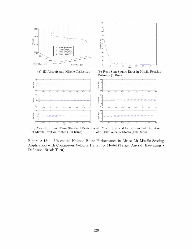
−2000

200400

600800

1000

−2000

−1000

0

1000

20003500

4000

4500

5000


Alti

tude

(m

)



0 0.05 0.1 0.15 0.2 0.25 0.3 0.35 0.40

5

10

15

20

25

30

35

40

45

50

posi

tion

erro

r (m

)

time (s)


0 0.05 0.1 0.15 0.2 0.25 0.3 0.35 0.4−50

0

50

x er

ror

(m)

0 0.05 0.1 0.15 0.2 0.25 0.3 0.35 0.4−50

0

50

y er

ror

(m)

0 0.05 0.1 0.15 0.2 0.25 0.3 0.35 0.4−50

0

50

z er

ror

(m)

time (s)


0 0.05 0.1 0.15 0.2 0.25 0.3 0.35 0.4−100

−50

0

50

100

vx e

rror

(m

/s)

0 0.05 0.1 0.15 0.2 0.25 0.3 0.35 0.4−100

−50

0

50

100

vy e

rror

(m

/s)

0 0.05 0.1 0.15 0.2 0.25 0.3 0.35 0.4−100

−50

0

50

100

vz e

rror

(m

/s)

time (s)


Figure A.13: Unscented Kalman Filter Performance in Air-to-Air Missile ScoringApplication with Continuous Velocity Dynamics Model (Target Aircraft Executing aDefensive Break Turn)

126

−2000

200400

600800

1000

−2000

−1000

0

1000

20003500

4000

4500

5000


Alti

tude

(m

)



0 0.05 0.1 0.15 0.2 0.25 0.3 0.35 0.40

5

10

15

20

25

30

35

40

45

50

posi

tion

erro

r (m

)time (s)


0 0.05 0.1 0.15 0.2 0.25 0.3 0.35 0.4−50

0

50

x er

ror

(m)

0 0.05 0.1 0.15 0.2 0.25 0.3 0.35 0.4−50

0

50

y er

ror

(m)

0 0.05 0.1 0.15 0.2 0.25 0.3 0.35 0.4−50

0

50

z er

ror

(m)

time (s)


0 0.05 0.1 0.15 0.2 0.25 0.3 0.35 0.4−100

−50

0

50

100

vx e

rror

(m

/s)

0 0.05 0.1 0.15 0.2 0.25 0.3 0.35 0.4−100

−50

0

50

100

vy e

rror

(m

/s)

0 0.05 0.1 0.15 0.2 0.25 0.3 0.35 0.4−100

−50

0

50

100

vz e

rror

(m

/s)

time (s)


Figure A.14: Unscented Kalman Filter Performance in Air-to-Air Missile ScoringApplication with Continuous Acceleration Dynamics Model (Target Aircraft Execut-ing a Defensive Break Turn)

127

−2000

200400

600800

1000

−2000

−1000

0

1000

20003500

4000

4500

5000


Alti

tude

(m

)



0 0.05 0.1 0.15 0.2 0.25 0.3 0.35 0.40

5

10

15

20

25

30

35

40

45

50

posi

tion

erro

r (m

)time (s)


0 0.05 0.1 0.15 0.2 0.25 0.3 0.35 0.4−50

0

50

x er

ror

(m)

0 0.05 0.1 0.15 0.2 0.25 0.3 0.35 0.4−50

0

50

y er

ror

(m)

0 0.05 0.1 0.15 0.2 0.25 0.3 0.35 0.4−50

0

50

z er

ror

(m)

time (s)


0 0.05 0.1 0.15 0.2 0.25 0.3 0.35 0.4−100

−50

0

50

100

vx e

rror

(m

/s)

0 0.05 0.1 0.15 0.2 0.25 0.3 0.35 0.4−100

−50

0

50

100

vy e

rror

(m

/s)

0 0.05 0.1 0.15 0.2 0.25 0.3 0.35 0.4−100

−50

0

50

100

vz e

rror

(m

/s)

time (s)


Figure A.15: Unscented Kalman Filter Performance in Air-to-Air Missile ScoringApplication with 3D Coordinated Turn Dynamics Model (Target Aircraft Executinga Defensive Break Turn)

128


Error Error Errorx -0.0005 m -0.0015 m -0.0017 my -0.0256 m -0.0097 m -0.0095 mz 0.0264 m 0.0123 m 0.0121 mvx 1.1089 m

s-0.0420 m

s-0.0551 m

s

vy 2.6419 ms

0.7519 ms

0.7275 ms

vz -2.0683 ms

-0.9832 ms

-0.9719 ms



s0.4983 m

s0.5138 m

s

vy 2.4432 ms

2.0602 ms

2.1214 ms

vz 2.5532 ms

2.0826 ms

2.1590 ms

129

−1000

−500

0

500

1000

−3000

−2000

−1000

0

10005000

5100

5200

5300

5400

5500


Alti

tude

(m

)



0 0.05 0.1 0.15 0.2 0.25 0.3 0.350

5

10

15

20

25

30

35

40

45

50

posi

tion

erro

r (m

)

time (s)


0 0.05 0.1 0.15 0.2 0.25 0.3 0.35−50

0

50

x er

ror

(m)

0 0.05 0.1 0.15 0.2 0.25 0.3 0.35−50

0

50

y er

ror

(m)

0 0.05 0.1 0.15 0.2 0.25 0.3 0.35−50

0

50

z er

ror

(m)

time (s)


0 0.05 0.1 0.15 0.2 0.25 0.3 0.35−100

−50

0

50

100

vx e

rror

(m

/s)

0 0.05 0.1 0.15 0.2 0.25 0.3 0.35−100

−50

0

50

100

vy e

rror

(m

/s)

0 0.05 0.1 0.15 0.2 0.25 0.3 0.35−100

−50

0

50

100

vz e

rror

(m

/s)

time (s)


Figure A.16: Unscented Kalman Filter Performance in Air-to-Air Missile ScoringApplication with Continuous Velocity Dynamics Model (Target Aircraft Executing aVertical Climb)

130

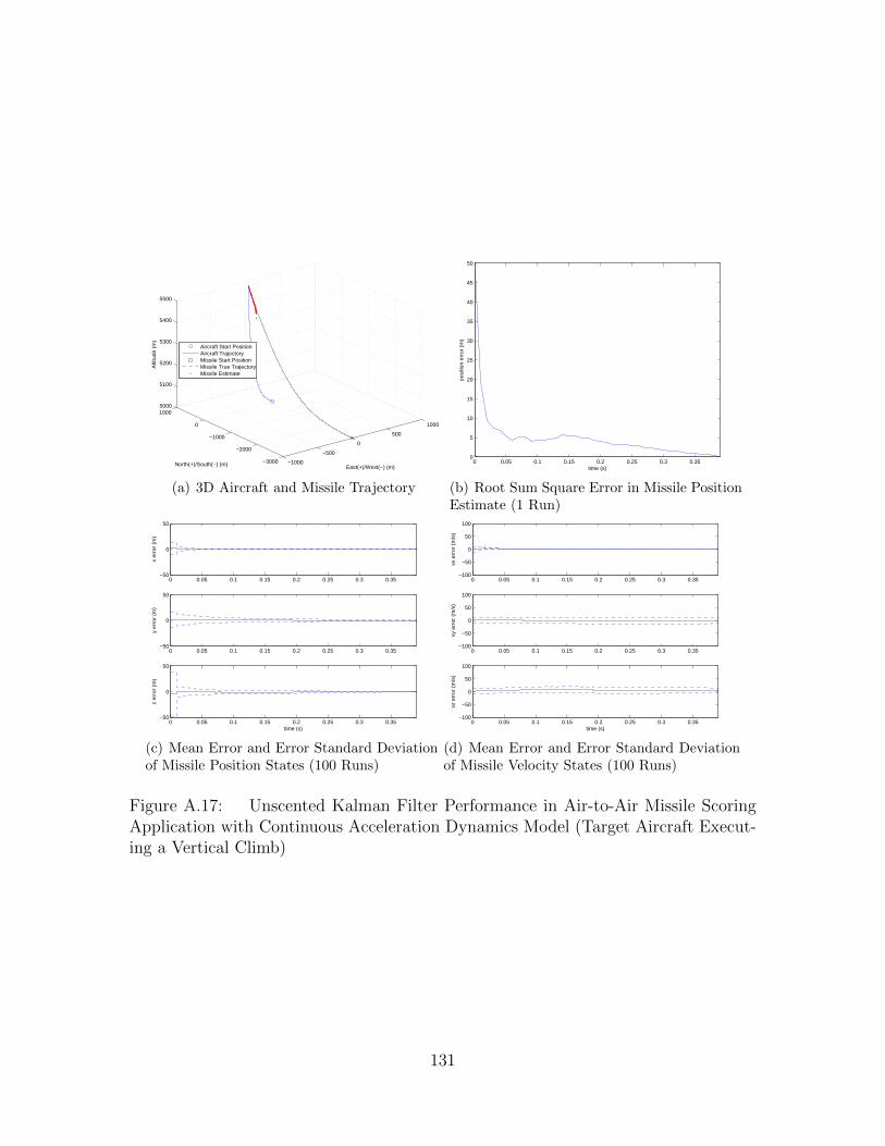
−1000

−500

0

500

1000

−3000

−2000

−1000

0

10005000

5100

5200

5300

5400

5500


Alti

tude

(m

)



0 0.05 0.1 0.15 0.2 0.25 0.3 0.350

5

10

15

20

25

30

35

40

45

50

posi

tion

erro

r (m

)time (s)


0 0.05 0.1 0.15 0.2 0.25 0.3 0.35−50

0

50

x er

ror

(m)

0 0.05 0.1 0.15 0.2 0.25 0.3 0.35−50

0

50

y er

ror

(m)

0 0.05 0.1 0.15 0.2 0.25 0.3 0.35−50

0

50

z er

ror

(m)

time (s)


0 0.05 0.1 0.15 0.2 0.25 0.3 0.35−100

−50

0

50

100

vx e

rror

(m

/s)

0 0.05 0.1 0.15 0.2 0.25 0.3 0.35−100

−50

0

50

100

vy e

rror

(m

/s)

0 0.05 0.1 0.15 0.2 0.25 0.3 0.35−100

−50

0

50

100

vz e

rror

(m

/s)

time (s)


Figure A.17: Unscented Kalman Filter Performance in Air-to-Air Missile ScoringApplication with Continuous Acceleration Dynamics Model (Target Aircraft Execut-ing a Vertical Climb)

131

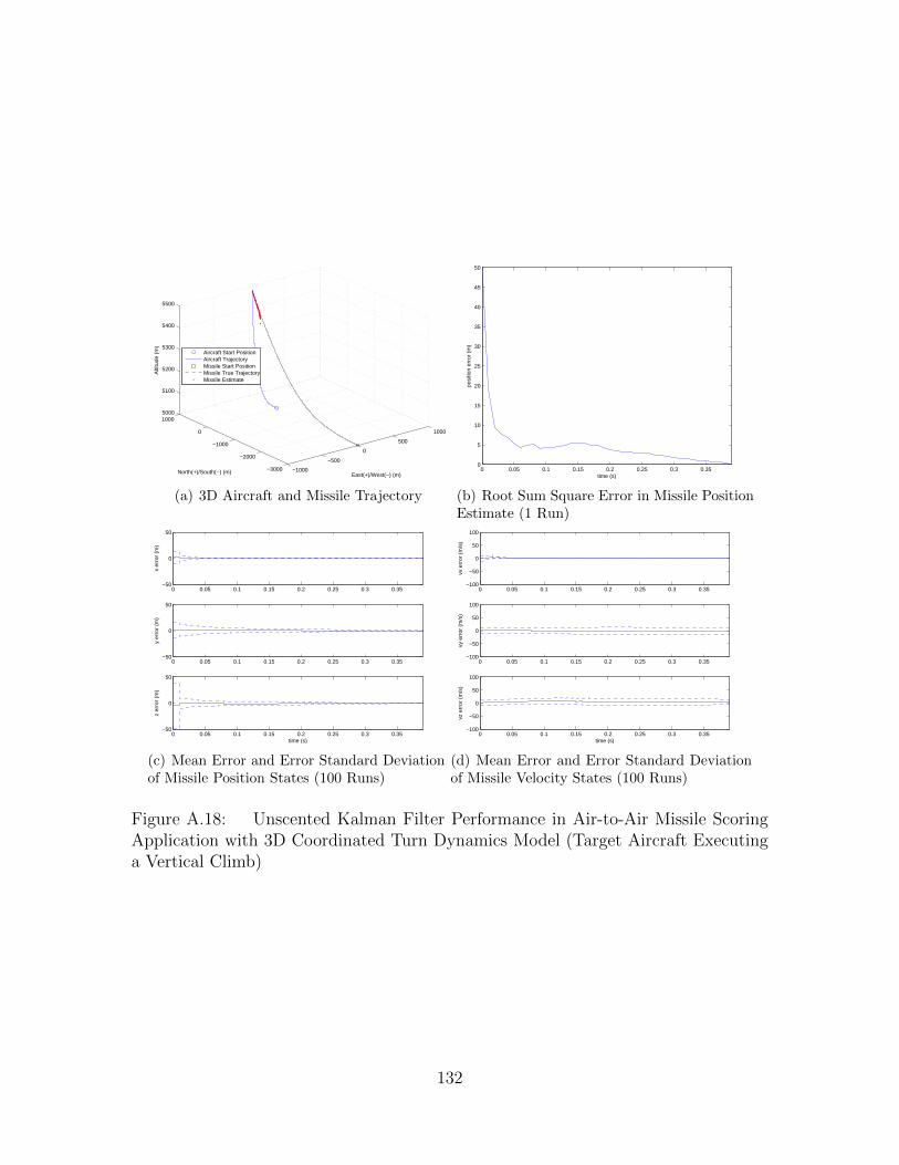
−1000

−500

0

500

1000

−3000

−2000

−1000

0

10005000

5100

5200

5300

5400

5500


Alti

tude

(m

)



0 0.05 0.1 0.15 0.2 0.25 0.3 0.350

5

10

15

20

25

30

35

40

45

50

posi

tion

erro

r (m

)time (s)


0 0.05 0.1 0.15 0.2 0.25 0.3 0.35−50

0

50

x er

ror

(m)

0 0.05 0.1 0.15 0.2 0.25 0.3 0.35−50

0

50

y er

ror

(m)

0 0.05 0.1 0.15 0.2 0.25 0.3 0.35−50

0

50

z er

ror

(m)

time (s)


0 0.05 0.1 0.15 0.2 0.25 0.3 0.35−100

−50

0

50

100

vx e

rror

(m

/s)

0 0.05 0.1 0.15 0.2 0.25 0.3 0.35−100

−50

0

50

100

vy e

rror

(m

/s)

0 0.05 0.1 0.15 0.2 0.25 0.3 0.35−100

−50

0

50

100

vz e

rror

(m

/s)

time (s)


Figure A.18: Unscented Kalman Filter Performance in Air-to-Air Missile ScoringApplication with 3D Coordinated Turn Dynamics Model (Target Aircraft Executinga Vertical Climb)

132


Error Error Errorx 0.0068 m -0.0007 m -0.0004 my -0.0068 m -0.0036 m -0.0026 mz -0.0634 m -0.0328 m -0.0302 mvx 0.6113 m

s-0.2165 m

s-0.2599 m

s

vy 0.5280 ms

0.2801 ms

0.2017 ms

vz 3.5622 ms

1.7507 ms

1.6033 ms



s0.4069 m

s0.4345 m

s

vy 8.4909 ms

8.6923 ms

9.0832 ms

vz 3.6732 ms

3.0559 ms

3.2494 ms

133

A.3 Particle Filter Simulations

−1500−1000

−5000

5001000

1500

0

500

1000

1500

2000

2500

30000

1000

2000

3000

4000

5000


Alti

tude

(m

)



0 0.05 0.1 0.15 0.2 0.25 0.3 0.35 0.4 0.450

5

10

15

20

25

30

35

40

45

50

posi

tion

erro

r (m

)

time (s)


0 0.05 0.1 0.15 0.2 0.25 0.3 0.35 0.4 0.45−50

0

50

x er

ror

(m)

0 0.05 0.1 0.15 0.2 0.25 0.3 0.35 0.4 0.45−50

0

50

y er

ror

(m)

0 0.05 0.1 0.15 0.2 0.25 0.3 0.35 0.4 0.45−50

0

50

z er

ror

(m)

time (s)


0 0.05 0.1 0.15 0.2 0.25 0.3 0.35 0.4 0.45−40

−20

0

20

40

vx e

rror

(m

/s)

0 0.05 0.1 0.15 0.2 0.25 0.3 0.35 0.4 0.45−40

−20

0

20

40

vy e

rror

(m

/s)

0 0.05 0.1 0.15 0.2 0.25 0.3 0.35 0.4 0.45−40

−20

0

20

40

vz e

rror

(m

/s)

time (s)


Figure A.19: Particle Filter Performance in Air-to-Air Missile Scoring Applicationwith Continuous Velocity Dynamics Model (Target Aircraft Non-maneuvering)

134

−1500−1000

−5000

5001000

1500

0

500

1000

1500

2000

2500

30000

1000

2000

3000

4000

5000


Alti

tude

(m

)



0 0.05 0.1 0.15 0.2 0.25 0.3 0.35 0.4 0.450

5

10

15

20

25

30

35

40

45

50

posi

tion

erro

r (m

)

time (s)


0 0.05 0.1 0.15 0.2 0.25 0.3 0.35 0.4 0.45−50

0

50

x er

ror

(m)

0 0.05 0.1 0.15 0.2 0.25 0.3 0.35 0.4 0.45−50

0

50

y er

ror

(m)

0 0.05 0.1 0.15 0.2 0.25 0.3 0.35 0.4 0.45−50

0

50

z er

ror

(m)

time (s)


0 0.05 0.1 0.15 0.2 0.25 0.3 0.35 0.4 0.45−40

−20

0

20

40

vx e

rror

(m

/s)

0 0.05 0.1 0.15 0.2 0.25 0.3 0.35 0.4 0.45−40

−20

0

20

40

vy e

rror

(m

/s)

0 0.05 0.1 0.15 0.2 0.25 0.3 0.35 0.4 0.45−40

−20

0

20

40

vz e

rror

(m

/s)

time (s)


Figure A.20: Particle Filter Performance in Air-to-Air Missile Scoring Applicationwith Continuous Acceleration Dynamics Model (Target Aircraft Non-maneuvering)

135

−1500−1000

−5000

5001000

1500

0

500

1000

1500

2000

2500

30000

1000

2000

3000

4000

5000


Alti

tude

(m

)



0 0.05 0.1 0.15 0.2 0.25 0.3 0.35 0.4 0.450

5

10

15

20

25

30

35

40

45

50

posi

tion

erro

r (m

)

time (s)


0 0.05 0.1 0.15 0.2 0.25 0.3 0.35 0.4 0.45−50

0

50

x er

ror

(m)

0 0.05 0.1 0.15 0.2 0.25 0.3 0.35 0.4 0.45−50

0

50

y er

ror

(m)

0 0.05 0.1 0.15 0.2 0.25 0.3 0.35 0.4 0.45−50

0

50

z er

ror

(m)

time (s)


0 0.05 0.1 0.15 0.2 0.25 0.3 0.35 0.4 0.45−40

−20

0

20

40

vx e

rror

(m

/s)

0 0.05 0.1 0.15 0.2 0.25 0.3 0.35 0.4 0.45−40

−20

0

20

40

vy e

rror

(m

/s)

0 0.05 0.1 0.15 0.2 0.25 0.3 0.35 0.4 0.45−40

−20

0

20

40

vz e

rror

(m

/s)

time (s)


Figure A.21: Particle Filter Performance in Air-to-Air Missile Scoring Applicationwith 3D Coordinated Turn Dynamics Model (Target Aircraft Non-maneuvering)

136

Table A.13: Comparison of Missile State Estimate Mean Error atImpact for Different Dynamics Models using a Particle Filter (Scenario1)Missile State CV Model Mean CA Model Mean CT Model Mean

Error Error Errorx 0.0086 m 0.0106 m -0.0135 my 0.0054 m 0.0103 m -0.0017 mz 0.0276 m -0.0024 m -0.0090 mvx -0.9277 m

s-0.8760 m

s0.4401 m

s

vy -0.3060 ms

-0.6064 ms

0.1163 ms

vz 2.5258 ms

2.1899 ms

1.6425 ms

Table A.14: Comparison of Missile State Estimate Error Standard Deviationat Impact for Different Dynamics Models using a Particle Filter (Scenario 1)Missile State CV Model Error CA Model Error CT Model Error


s13.8147 m

s13.4921 m

s

vy 19.3195 ms

28.5924 ms

24.0229 ms

vz 3.1860 ms

3.7043 ms

3.3387 ms

137

−2000

200400

600800

1000

−2000

−1000

0

1000

20003500

4000

4500

5000


Alti

tude

(m

)



0 0.05 0.1 0.15 0.2 0.25 0.3 0.35 0.40

5

10

15

20

25

30

35

40

45

50

posi

tion

erro

r (m

)

time (s)


0 0.05 0.1 0.15 0.2 0.25 0.3 0.35 0.4−50

0

50

x er

ror

(m)

0 0.05 0.1 0.15 0.2 0.25 0.3 0.35 0.4−50

0

50

y er

ror

(m)

0 0.05 0.1 0.15 0.2 0.25 0.3 0.35 0.4−50

0

50

z er

ror

(m)

time (s)


0 0.05 0.1 0.15 0.2 0.25 0.3 0.35 0.4−100

−50

0

50

100

vx e

rror

(m

/s)

0 0.05 0.1 0.15 0.2 0.25 0.3 0.35 0.4−100

−50

0

50

100

vy e

rror

(m

/s)

0 0.05 0.1 0.15 0.2 0.25 0.3 0.35 0.4−100

−50

0

50

100

vz e

rror

(m

/s)

time (s)


Figure A.22: Particle Filter Performance in Air-to-Air Missile Scoring Applicationwith Continuous Velocity Dynamics Model (Target Aircraft Executing a DefensiveBreak Turn)

138

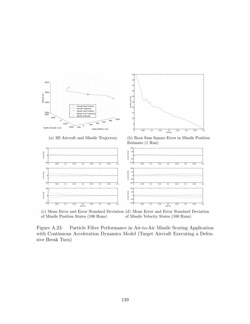
−2000

200400

600800

1000

−2000

−1000

0

1000

20003500

4000

4500

5000


Alti

tude

(m

)



0 0.05 0.1 0.15 0.2 0.25 0.3 0.35 0.40

5

10

15

20

25

30

35

40

45

50

posi

tion

erro

r (m

)time (s)


0 0.05 0.1 0.15 0.2 0.25 0.3 0.35 0.4−50

0

50

x er

ror

(m)

0 0.05 0.1 0.15 0.2 0.25 0.3 0.35 0.4−50

0

50

y er

ror

(m)

0 0.05 0.1 0.15 0.2 0.25 0.3 0.35 0.4−50

0

50

z er

ror

(m)

time (s)


0 0.05 0.1 0.15 0.2 0.25 0.3 0.35 0.4−100

−50

0

50

100

vx e

rror

(m

/s)

0 0.05 0.1 0.15 0.2 0.25 0.3 0.35 0.4−100

−50

0

50

100

vy e

rror

(m

/s)

0 0.05 0.1 0.15 0.2 0.25 0.3 0.35 0.4−100

−50

0

50

100

vz e

rror

(m

/s)

time (s)


Figure A.23: Particle Filter Performance in Air-to-Air Missile Scoring Applicationwith Continuous Acceleration Dynamics Model (Target Aircraft Executing a Defen-sive Break Turn)

139

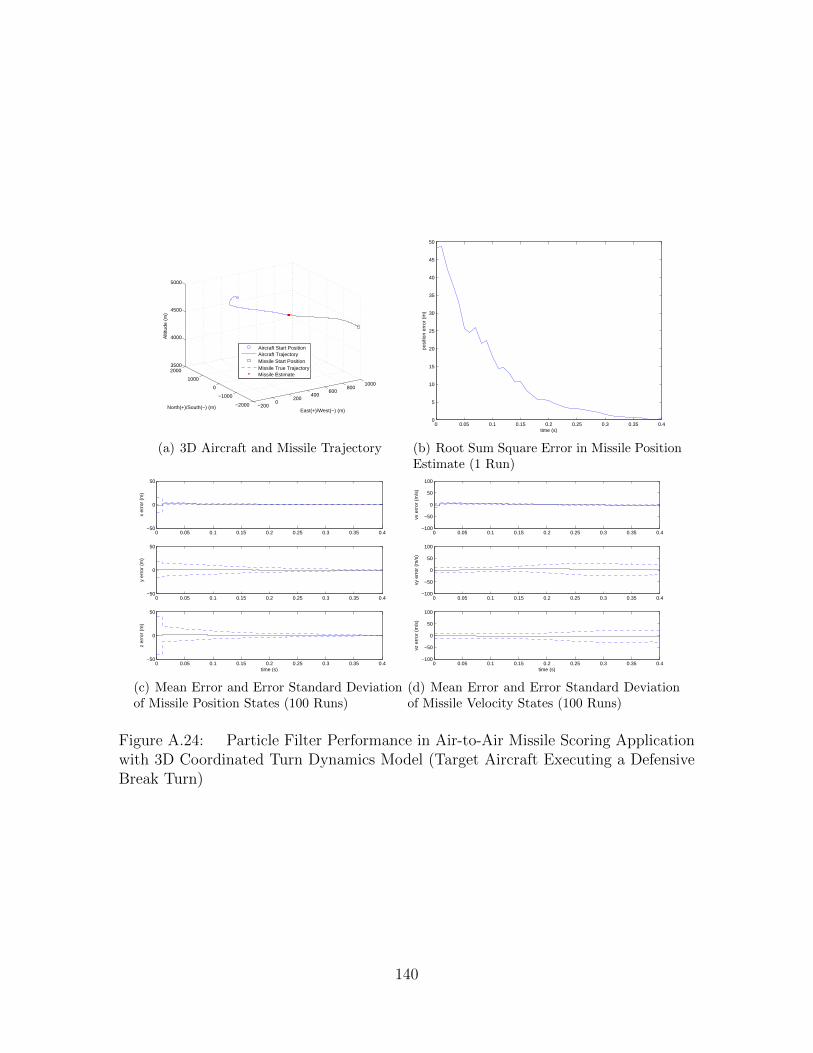
−2000

200400

600800

1000

−2000

−1000

0

1000

20003500

4000

4500

5000


Alti

tude

(m

)



0 0.05 0.1 0.15 0.2 0.25 0.3 0.35 0.40

5

10

15

20

25

30

35

40

45

50

posi

tion

erro

r (m

)time (s)


0 0.05 0.1 0.15 0.2 0.25 0.3 0.35 0.4−50

0

50

x er

ror

(m)

0 0.05 0.1 0.15 0.2 0.25 0.3 0.35 0.4−50

0

50

y er

ror

(m)

0 0.05 0.1 0.15 0.2 0.25 0.3 0.35 0.4−50

0

50

z er

ror

(m)

time (s)


0 0.05 0.1 0.15 0.2 0.25 0.3 0.35 0.4−100

−50

0

50

100

vx e

rror

(m

/s)

0 0.05 0.1 0.15 0.2 0.25 0.3 0.35 0.4−100

−50

0

50

100

vy e

rror

(m

/s)

0 0.05 0.1 0.15 0.2 0.25 0.3 0.35 0.4−100

−50

0

50

100

vz e

rror

(m

/s)

time (s)


Figure A.24: Particle Filter Performance in Air-to-Air Missile Scoring Applicationwith 3D Coordinated Turn Dynamics Model (Target Aircraft Executing a DefensiveBreak Turn)

140


Error Error Errorx 0.0054 m 0.0133 m 0.0140 my -0.0162 m 0.0153 m 0.0261 mz 0.0358 m 0.0080 m 0.0064 mvx 0.0909 m

s-0.6431 m

s-0.7438 m

s

vy 1.7767 ms

-0.6020 ms

-1.0024 ms

vz -2.6757 ms

-0.0664 ms

-0.6370 ms



s4.8930 m

s3.7204 m

s

vy 9.4397 ms

20.4866 ms

16.6840 ms

vz 10.3529 ms

22.7754 ms

22.7241 ms

141

−1000

−500

0

500

1000

−3000

−2000

−1000

0

10005000

5100

5200

5300

5400

5500


Alti

tude

(m

)



0 0.05 0.1 0.15 0.2 0.25 0.3 0.350

5

10

15

20

25

30

35

40

45

50

posi

tion

erro

r (m

)

time (s)


0 0.05 0.1 0.15 0.2 0.25 0.3 0.35−50

0

50

x er

ror

(m)

0 0.05 0.1 0.15 0.2 0.25 0.3 0.35−50

0

50

y er

ror

(m)

0 0.05 0.1 0.15 0.2 0.25 0.3 0.35−50

0

50

z er

ror

(m)

time (s)


0 0.05 0.1 0.15 0.2 0.25 0.3 0.35−100

−50

0

50

100

vx e

rror

(m

/s)

0 0.05 0.1 0.15 0.2 0.25 0.3 0.35−100

−50

0

50

100

vy e

rror

(m

/s)

0 0.05 0.1 0.15 0.2 0.25 0.3 0.35−100

−50

0

50

100

vz e

rror

(m

/s)

time (s)


Figure A.25: Particle Filter Performance in Air-to-Air Missile Scoring Applica-tion with Continuous Velocity Dynamics Model (Target Aircraft Executing a VerticalClimb)

142

−1000

−500

0

500

1000

−3000

−2000

−1000

0

10005000

5100

5200

5300

5400

5500


Alti

tude

(m

)



0 0.05 0.1 0.15 0.2 0.25 0.3 0.350

5

10

15

20

25

30

35

40

45

50

posi

tion

erro

r (m

)time (s)


0 0.05 0.1 0.15 0.2 0.25 0.3 0.35−50

0

50

x er

ror

(m)

0 0.05 0.1 0.15 0.2 0.25 0.3 0.35−50

0

50

y er

ror

(m)

0 0.05 0.1 0.15 0.2 0.25 0.3 0.35−50

0

50

z er

ror

(m)

time (s)


0 0.05 0.1 0.15 0.2 0.25 0.3 0.35−100

−50

0

50

100

vx e

rror

(m

/s)

0 0.05 0.1 0.15 0.2 0.25 0.3 0.35−100

−50

0

50

100

vy e

rror

(m

/s)

0 0.05 0.1 0.15 0.2 0.25 0.3 0.35−100

−50

0

50

100

vz e

rror

(m

/s)

time (s)


Figure A.26: Particle Filter Performance in Air-to-Air Missile Scoring Applicationwith Continuous Acceleration Dynamics Model (Target Aircraft Executing a VerticalClimb)

143

−1000

−500

0

500

1000

−3000

−2000

−1000

0

10005000

5100

5200

5300

5400

5500


Alti

tude

(m

)



0 0.05 0.1 0.15 0.2 0.25 0.3 0.350

5

10

15

20

25

30

35

40

45

50

posi

tion

erro

r (m

)time (s)


0 0.05 0.1 0.15 0.2 0.25 0.3 0.35−50

0

50

x er

ror

(m)

0 0.05 0.1 0.15 0.2 0.25 0.3 0.35−50

0

50

y er

ror

(m)

0 0.05 0.1 0.15 0.2 0.25 0.3 0.35−50

0

50

z er

ror

(m)

time (s)


0 0.05 0.1 0.15 0.2 0.25 0.3 0.35−100

−50

0

50

100

vx e

rror

(m

/s)

0 0.05 0.1 0.15 0.2 0.25 0.3 0.35−100

−50

0

50

100

vy e

rror

(m

/s)

0 0.05 0.1 0.15 0.2 0.25 0.3 0.35−100

−50

0

50

100

vz e

rror

(m

/s)

time (s)


Figure A.27: Particle Filter Performance in Air-to-Air Missile Scoring Applicationwith 3D Coordinated Turn Dynamics Model (Target Aircraft Executing a VerticalClimb)

144


Error Error Errorx 0.0031 m 0.0202 m 0.0112 my 0.0260 m 0.0555 m -0.0026 mz -0.0705 m -0.0791 m -0.0340 mvx -1.1108 m

s-1.3862 m

s-1.9890 m

s

vy -2.0372 ms

-4.2506 ms

0.1984 ms

vz 3.6544 ms

4.5102 ms

1.5529 ms



s2.9458 m

s3.3191 m

s

vy 20.8787 ms

33.5605 ms

36.3426 ms

vz 9.4543 ms

19.3589 ms

17.3036 ms

145

Appendix B. Flight Test Results

B.1 Sensor Geometry: 90◦ Aspect Angle

0 0.2 0.4 0.6 0.8 1 1.2 1.4 1.6 1.8 20

20

40

60

80

100

120

Time (s)

RS

S P

ositi

on E

rror

(m

)


(a) Root Sum Square Error in Surrogate MissilePosition Estimate

0 0.2 0.4 0.6 0.8 1 1.2 1.4 1.6 1.8 20

10

20

30

40

50

60

70

80

Time (s)

RS

S V

eloc

ity E

rror

(m

/s)


(b) Root Sum Square Error in Surrogate MissileVelocity Estimate

0 0.2 0.4 0.6 0.8 1 1.2 1.4 1.6 1.8 20

20

40

60

80

100

120

140

160

180

200

Time (s)

Sla

nt R

ange

(m

)


(c) Radar Sensors Slant Range Measurements

0 0.2 0.4 0.6 0.8 1 1.2 1.4 1.6 1.8 20

10

20

30

40

50

60

70

80

Time (s)

Vel

ocity

(m

/s)


(d) Radar Sensors Speed Measurements

Figure B.1: Air-to-Air Missile Scoring System Performance in Scoring C-12 Surro-gate Missile using an Unscented Kalman Filter with Continuous Dynamics VelocityModel (90◦ Drone Aspect Angle / Run 1)

146

0 0.5 1 1.5 20

20

40

60

80

100

120

Time (s)

RS

S P

ositi

on E

rror

(m

)



0 0.5 1 1.5 20

10

20

30

40

50

60

70

80

Time (s)

RS

S V

eloc

ity E

rror

(m

/s)



0 0.5 1 1.5 20

20

40

60

80

100

120

140

160

180

200

Time (s)

Sla

nt R

ange

(m

)



0 0.5 1 1.5 20

10

20

30

40

50

60

70

80

Time (s)

Vel

ocity

(m

/s)




147

0 0.5 1 1.5 20

20

40

60

80

100

120

Time (s)

RS

S P

ositi

on E

rror

(m

)



0 0.5 1 1.5 20

10

20

30

40

50

60

70

80

Time (s)

RS

S V

eloc

ity E

rror

(m

/s)



0 0.5 1 1.5 20

20

40

60

80

100

120

140

160

180

200

Time (s)

Sla

nt R

ange

(m

)



0 0.5 1 1.5 20

10

20

30

40

50

60

70

80

Time (s)

Vel

ocity

(m

/s)




148

0 0.5 1 1.5 2 2.5 30

20

40

60

80

100

120

Time (s)

RS

S P

ositi

on E

rror

(m

)



0 0.5 1 1.5 2 2.5 30

10

20

30

40

50

60

70

80

Time (s)

RS

S V

eloc

ity E

rror

(m

/s)



0 0.5 1 1.5 2 2.5 30

20

40

60

80

100

120

140

160

180

200

Time (s)

Sla

nt R

ange

(m

)



0 0.5 1 1.5 2 2.5 30

10

20

30

40

50

60

70

80

Time (s)

Vel

ocity

(m

/s)




149

0 0.5 1 1.5 2 2.50

20

40

60

80

100

120

Time (s)

RS

S P

ositi

on E

rror

(m

)



0 0.5 1 1.5 2 2.50

10

20

30

40

50

60

70

80

Time (s)

RS

S V

eloc

ity E

rror

(m

/s)



0 0.5 1 1.5 2 2.50

20

40

60

80

100

120

140

160

180

200

Time (s)

Sla

nt R

ange

(m

)



0 0.5 1 1.5 2 2.50

10

20

30

40

50

60

70

80

Time (s)

Vel

ocity

(m

/s)




150

0 0.5 1 1.5 20

20

40

60

80

100

120

Time (s)

RS

S P

ositi

on E

rror

(m

)



0 0.5 1 1.5 20

10

20

30

40

50

60

70

80

Time (s)

RS

S V

eloc

ity E

rror

(m

/s)



0 0.5 1 1.5 20

20

40

60

80

100

120

140

160

180

200

Time (s)

Sla

nt R

ange

(m

)



0 0.5 1 1.5 20

10

20

30

40

50

60

70

80

Time (s)

Vel

ocity

(m

/s)




151

0 0.5 1 1.5 2 2.50

20

40

60

80

100

120

Time (s)

RS

S P

ositi

on E

rror

(m

)



0 0.5 1 1.5 2 2.50

10

20

30

40

50

60

70

80

Time (s)

RS

S V

eloc

ity E

rror

(m

/s)



0 0.5 1 1.5 2 2.50

20

40

60

80

100

120

140

160

180

200

Time (s)

Sla

nt R

ange

(m

)



0 0.5 1 1.5 2 2.50

10

20

30

40

50

60

70

80

Time (s)

Vel

ocity

(m

/s)




152

0 0.5 1 1.5 20

20

40

60

80

100

120

Time (s)

RS

S P

ositi

on E

rror

(m

)



0 0.5 1 1.5 20

10

20

30

40

50

60

70

80

Time (s)

RS

S V

eloc

ity E

rror

(m

/s)



0 0.5 1 1.5 20

20

40

60

80

100

120

140

160

180

200

Time (s)

Sla

nt R

ange

(m

)



0 0.5 1 1.5 20

10

20

30

40

50

60

70

80

Time (s)

Vel

ocity

(m

/s)




153

0 0.5 1 1.5 20

20

40

60

80

100

120

Time (s)

RS

S P

ositi

on E

rror

(m

)



0 0.5 1 1.5 20

10

20

30

40

50

60

70

80

Time (s)

RS

S V

eloc

ity E

rror

(m

/s)



0 0.5 1 1.5 20

20

40

60

80

100

120

140

160

180

200

Time (s)

Sla

nt R

ange

(m

)



0 0.5 1 1.5 20

10

20

30

40

50

60

70

80

Time (s)

Vel

ocity

(m

/s)




154

0 0.5 1 1.5 2 2.50

20

40

60

80

100

120

Time (s)

RS

S P

ositi

on E

rror

(m

)



0 0.5 1 1.5 2 2.50

10

20

30

40

50

60

70

80

Time (s)

RS

S V

eloc

ity E

rror

(m

/s)



0 0.5 1 1.5 2 2.50

20

40

60

80

100

120

140

160

180

200

Time (s)

Sla

nt R

ange

(m

)



0 0.5 1 1.5 2 2.50

10

20

30

40

50

60

70

80

Time (s)

Vel

ocity

(m

/s)



Figure B.10: Air-to-Air Missile Scoring System Performance in Scoring C-12 Sur-rogate Missile using an Unscented Kalman Filter with Continuous Dynamics VelocityModel (90◦ Drone Aspect Angle / Run 10)

155

0 0.5 1 1.5 2 2.50

20

40

60

80

100

120

Time (s)

RS

S P

ositi

on E

rror

(m

)



0 0.5 1 1.5 2 2.50

10

20

30

40

50

60

70

80

Time (s)

RS

S V

eloc

ity E

rror

(m

/s)



0 0.5 1 1.5 2 2.50

20

40

60

80

100

120

140

160

180

200

Time (s)

Sla

nt R

ange

(m

)



0 0.5 1 1.5 2 2.50

10

20

30

40

50

60

70

80

Time (s)

Vel

ocity

(m

/s)




156

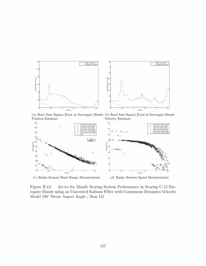
0 0.5 1 1.5 2 2.50

20

40

60

80

100

120

Time (s)

RS

S P

ositi

on E

rror

(m

)



0 0.5 1 1.5 2 2.50

10

20

30

40

50

60

70

80

Time (s)

RS

S V

eloc

ity E

rror

(m

/s)



0 0.5 1 1.5 2 2.50

20

40

60

80

100

120

140

160

180

200

Time (s)

Sla

nt R

ange

(m

)



0 0.5 1 1.5 2 2.50

10

20

30

40

50

60

70

80

Time (s)

Vel

ocity

(m

/s)




157

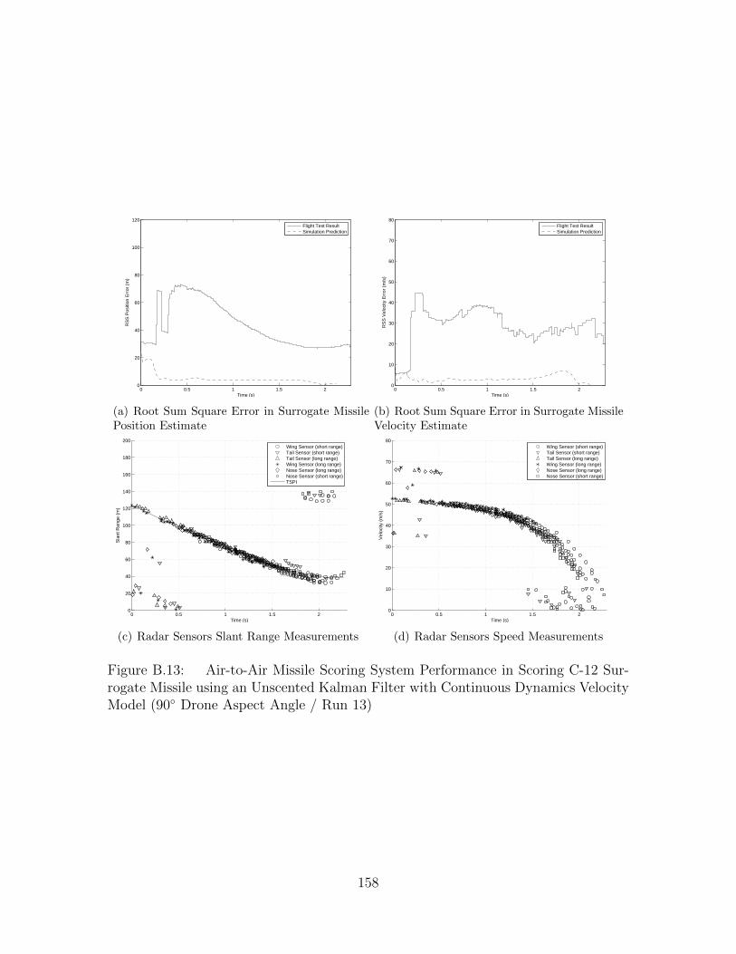
0 0.5 1 1.5 20

20

40

60

80

100

120

Time (s)

RS

S P

ositi

on E

rror

(m

)



0 0.5 1 1.5 20

10

20

30

40

50

60

70

80

Time (s)

RS

S V

eloc

ity E

rror

(m

/s)



0 0.5 1 1.5 20

20

40

60

80

100

120

140

160

180

200

Time (s)

Sla

nt R

ange

(m

)



0 0.5 1 1.5 20

10

20

30

40

50

60

70

80

Time (s)

Vel

ocity

(m

/s)




158

0 0.5 1 1.5 2 2.50

20

40

60

80

100

120

Time (s)

RS

S P

ositi

on E

rror

(m

)



0 0.5 1 1.5 2 2.50

10

20

30

40

50

60

70

80

Time (s)

RS

S V

eloc

ity E

rror

(m

/s)



0 0.5 1 1.5 2 2.50

20

40

60

80

100

120

140

160

180

200

Time (s)

Sla

nt R

ange

(m

)



0 0.5 1 1.5 2 2.50

10

20

30

40

50

60

70

80

Time (s)

Vel

ocity

(m

/s)




159

0 0.2 0.4 0.6 0.8 1 1.2 1.4 1.6 1.8 20

20

40

60

80

100

120

Time (s)

RS

S P

ositi

on E

rror

(m

)



0 0.2 0.4 0.6 0.8 1 1.2 1.4 1.6 1.8 20

10

20

30

40

50

60

70

80

Time (s)

RS

S V

eloc

ity E

rror

(m

/s)



0 0.2 0.4 0.6 0.8 1 1.2 1.4 1.6 1.8 20

20

40

60

80

100

120

140

160

180

200

Time (s)

Sla

nt R

ange

(m

)



0 0.2 0.4 0.6 0.8 1 1.2 1.4 1.6 1.8 20

10

20

30

40

50

60

70

80

Time (s)

Vel

ocity

(m

/s)




160


0 0.5 1 1.5 2 2.50

20

40

60

80

100

120

Time (s)

RS

S P

ositi

on E

rror

(m

)



0 0.5 1 1.5 2 2.50

10

20

30

40

50

60

70

80

Time (s)

RS

S V

eloc

ity E

rror

(m

/s)



0 0.5 1 1.5 2 2.50

20

40

60

80

100

120

140

160

180

200

Time (s)

Sla

nt R

ange

(m

)



0 0.5 1 1.5 2 2.50

10

20

30

40

50

60

70

80

Time (s)

Vel

ocity

(m

/s)




161

0 0.2 0.4 0.6 0.8 1 1.2 1.4 1.6 1.8 20

20

40

60

80

100

120

Time (s)

RS

S P

ositi

on E

rror

(m

)



0 0.2 0.4 0.6 0.8 1 1.2 1.4 1.6 1.8 20

10

20

30

40

50

60

70

80

Time (s)

RS

S V

eloc

ity E

rror

(m

/s)



0 0.2 0.4 0.6 0.8 1 1.2 1.4 1.6 1.8 20

20

40

60

80

100

120

140

160

180

200

Time (s)

Sla

nt R

ange

(m

)



0 0.2 0.4 0.6 0.8 1 1.2 1.4 1.6 1.8 20

10

20

30

40

50

60

70

80

Time (s)

Vel

ocity

(m

/s)




162

0 0.5 1 1.5 2 2.50

20

40

60

80

100

120

Time (s)

RS

S P

ositi

on E

rror

(m

)



0 0.5 1 1.5 2 2.50

10

20

30

40

50

60

70

80

Time (s)

RS

S V

eloc

ity E

rror

(m

/s)



0 0.5 1 1.5 2 2.50

20

40

60

80

100

120

140

160

180

200

Time (s)

Sla

nt R

ange

(m

)



0 0.5 1 1.5 2 2.50

10

20

30

40

50

60

70

80

Time (s)

Vel

ocity

(m

/s)




163

0 0.2 0.4 0.6 0.8 1 1.2 1.4 1.6 1.8 20

20

40

60

80

100

120

Time (s)

RS

S P

ositi

on E

rror

(m

)



0 0.2 0.4 0.6 0.8 1 1.2 1.4 1.6 1.8 20

10

20

30

40

50

60

70

80

Time (s)

RS

S V

eloc

ity E

rror

(m

/s)



0 0.2 0.4 0.6 0.8 1 1.2 1.4 1.6 1.8 20

20

40

60

80

100

120

140

160

180

200

Time (s)

Sla

nt R

ange

(m

)



0 0.2 0.4 0.6 0.8 1 1.2 1.4 1.6 1.8 20

10

20

30

40

50

60

70

80

Time (s)

Vel

ocity

(m

/s)




164

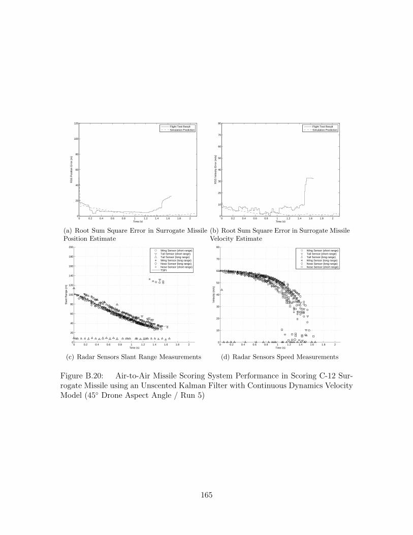
0 0.2 0.4 0.6 0.8 1 1.2 1.4 1.6 1.8 20

20

40

60

80

100

120

Time (s)

RS

S P

ositi

on E

rror

(m

)



0 0.2 0.4 0.6 0.8 1 1.2 1.4 1.6 1.8 20

10

20

30

40

50

60

70

80

Time (s)

RS

S V

eloc

ity E

rror

(m

/s)



0 0.2 0.4 0.6 0.8 1 1.2 1.4 1.6 1.8 20

20

40

60

80

100

120

140

160

180

200

Time (s)

Sla

nt R

ange

(m

)



0 0.2 0.4 0.6 0.8 1 1.2 1.4 1.6 1.8 20

10

20

30

40

50

60

70

80

Time (s)

Vel

ocity

(m

/s)




165

0 0.2 0.4 0.6 0.8 1 1.2 1.4 1.6 1.8 20

20

40

60

80

100

120

Time (s)

RS

S P

ositi

on E

rror

(m

)



0 0.2 0.4 0.6 0.8 1 1.2 1.4 1.6 1.8 20

10

20

30

40

50

60

70

80

Time (s)

RS

S V

eloc

ity E

rror

(m

/s)



0 0.2 0.4 0.6 0.8 1 1.2 1.4 1.6 1.8 20

20

40

60

80

100

120

140

160

180

200

Time (s)

Sla

nt R

ange

(m

)



0 0.2 0.4 0.6 0.8 1 1.2 1.4 1.6 1.8 20

10

20

30

40

50

60

70

80

Time (s)

Vel

ocity

(m

/s)




166

0 0.2 0.4 0.6 0.8 1 1.2 1.4 1.6 1.8 20

20

40

60

80

100

120

Time (s)

RS

S P

ositi

on E

rror

(m

)



0 0.2 0.4 0.6 0.8 1 1.2 1.4 1.6 1.8 20

10

20

30

40

50

60

70

80

Time (s)

RS

S V

eloc

ity E

rror

(m

/s)



0 0.2 0.4 0.6 0.8 1 1.2 1.4 1.6 1.8 20

20

40

60

80

100

120

140

160

180

200

Time (s)

Sla

nt R

ange

(m

)



0 0.2 0.4 0.6 0.8 1 1.2 1.4 1.6 1.8 20

10

20

30

40

50

60

70

80

Time (s)

Vel

ocity

(m

/s)




167

0 0.5 1 1.5 2 2.50

20

40

60

80

100

120

140

Time (s)

RS

S P

ositi

on E

rror

(m

)



0 0.5 1 1.5 20

10

20

30

40

50

60

70

80

Time (s)

RS

S V

eloc

ity E

rror

(m

/s)



0 0.5 1 1.5 2 2.50

20

40

60

80

100

120

140

160

180

200

Time (s)

Sla

nt R

ange

(m

)



0 0.5 1 1.5 20

10

20

30

40

50

60

70

80

Time (s)

Vel

ocity

(m

/s)




168

0 0.5 1 1.5 2 2.50

20

40

60

80

100

120

Time (s)

RS

S P

ositi

on E

rror

(m

)



0 0.5 1 1.5 2 2.50

10

20

30

40

50

60

70

80

Time (s)

RS

S V

eloc

ity E

rror

(m

/s)



0 0.5 1 1.5 2 2.50

20

40

60

80

100

120

140

160

180

200

Time (s)

Sla

nt R

ange

(m

)



0 0.5 1 1.5 2 2.50

10

20

30

40

50

60

70

80

Time (s)

Vel

ocity

(m

/s)




169

0 0.2 0.4 0.6 0.8 1 1.2 1.4 1.6 1.8 20

20

40

60

80

100

120

Time (s)

RS

S P

ositi

on E

rror

(m

)



0 0.2 0.4 0.6 0.8 1 1.2 1.4 1.6 1.8 20

10

20

30

40

50

60

70

80

Time (s)

RS

S V

eloc

ity E

rror

(m

/s)



0 0.2 0.4 0.6 0.8 1 1.2 1.4 1.6 1.8 20

20

40

60

80

100

120

140

160

180

200

Time (s)

Sla

nt R

ange

(m

)



0 0.2 0.4 0.6 0.8 1 1.2 1.4 1.6 1.8 20

10

20

30

40

50

60

70

80

Time (s)

Vel

ocity

(m

/s)




170

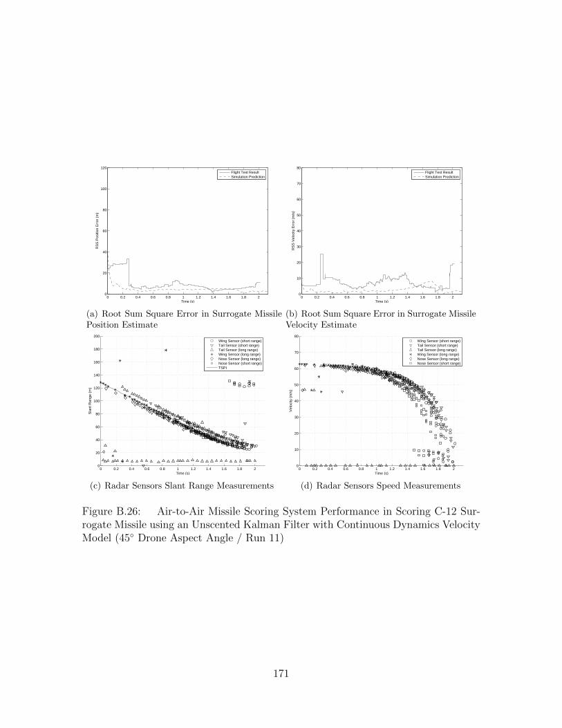
0 0.2 0.4 0.6 0.8 1 1.2 1.4 1.6 1.8 20

20

40

60

80

100

120

Time (s)

RS

S P

ositi

on E

rror

(m

)



0 0.2 0.4 0.6 0.8 1 1.2 1.4 1.6 1.8 20

10

20

30

40

50

60

70

80

Time (s)

RS

S V

eloc

ity E

rror

(m

/s)



0 0.2 0.4 0.6 0.8 1 1.2 1.4 1.6 1.8 20

20

40

60

80

100

120

140

160

180

200

Time (s)

Sla

nt R

ange

(m

)



0 0.2 0.4 0.6 0.8 1 1.2 1.4 1.6 1.8 20

10

20

30

40

50

60

70

80

Time (s)

Vel

ocity

(m

/s)




171

0 0.2 0.4 0.6 0.8 1 1.2 1.4 1.6 1.8 20

20

40

60

80

100

120

Time (s)

RS

S P

ositi

on E

rror

(m

)



0 0.2 0.4 0.6 0.8 1 1.2 1.4 1.6 1.8 20

10

20

30

40

50

60

70

80

Time (s)

RS

S V

eloc

ity E

rror

(m

/s)



0 0.2 0.4 0.6 0.8 1 1.2 1.4 1.6 1.8 20

20

40

60

80

100

120

140

160

180

200

Time (s)

Sla

nt R

ange

(m

)



0 0.2 0.4 0.6 0.8 1 1.2 1.4 1.6 1.8 20

10

20

30

40

50

60

70

80

Time (s)

Vel

ocity

(m

/s)




172

0 0.5 1 1.5 20

20

40

60

80

100

120

Time (s)

RS

S P

ositi

on E

rror

(m

)



0 0.5 1 1.5 20

10

20

30

40

50

60

70

80

Time (s)

RS

S V

eloc

ity E

rror

(m

/s)



0 0.5 1 1.5 20

20

40

60

80

100

120

140

160

180

200

Time (s)

Sla

nt R

ange

(m

)



0 0.5 1 1.5 20

10

20

30

40

50

60

70

80

Time (s)

Vel

ocity

(m

/s)




173

0 0.2 0.4 0.6 0.8 1 1.2 1.4 1.6 1.8 20

20

40

60

80

100

120

Time (s)

RS

S P

ositi

on E

rror

(m

)



0 0.2 0.4 0.6 0.8 1 1.2 1.4 1.6 1.8 20

10

20

30

40

50

60

70

80

Time (s)

RS

S V

eloc

ity E

rror

(m

/s)



0 0.2 0.4 0.6 0.8 1 1.2 1.4 1.6 1.8 20

20

40

60

80

100

120

140

160

180

200

Time (s)

Sla

nt R

ange

(m

)



0 0.2 0.4 0.6 0.8 1 1.2 1.4 1.6 1.8 20

10

20

30

40

50

60

70

80

Time (s)

Vel

ocity

(m

/s)




174

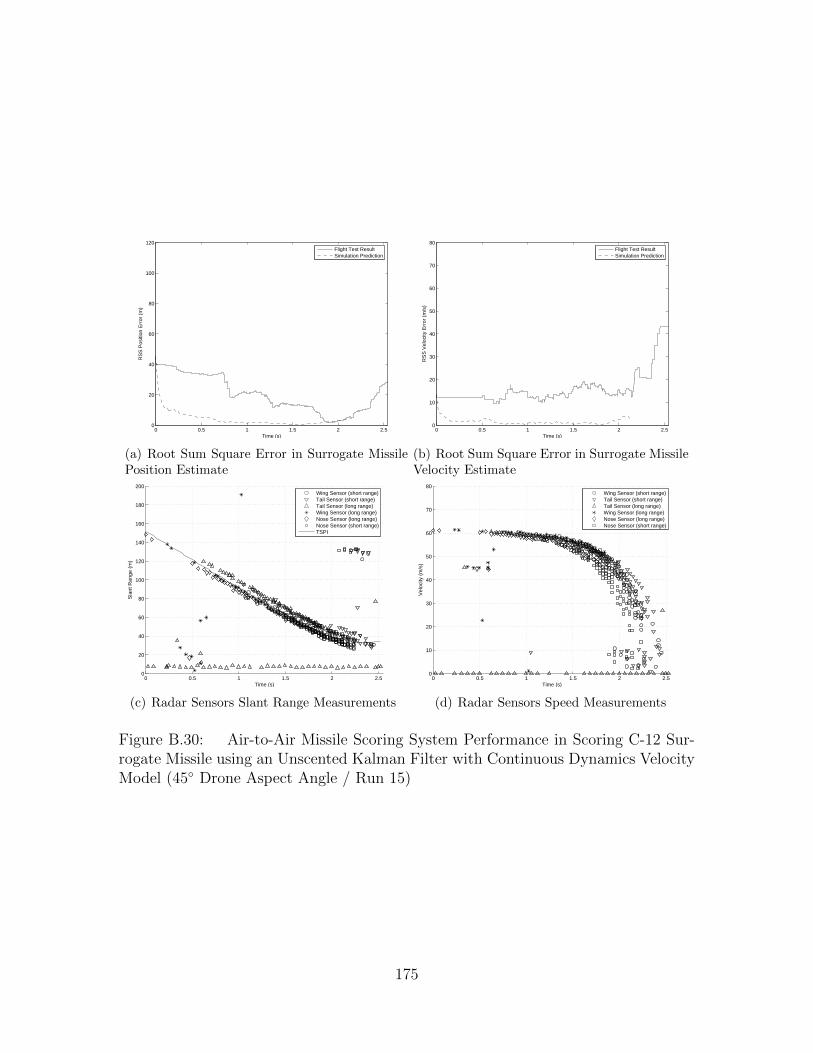
0 0.5 1 1.5 2 2.50

20

40

60

80

100

120

Time (s)

RS

S P

ositi

on E

rror

(m

)



0 0.5 1 1.5 2 2.50

10

20

30

40

50

60

70

80

Time (s)

RS

S V

eloc

ity E

rror

(m

/s)



0 0.5 1 1.5 2 2.50

20

40

60

80

100

120

140

160

180

200

Time (s)

Sla

nt R

ange

(m

)



0 0.5 1 1.5 2 2.50

10

20

30

40

50

60

70

80

Time (s)

Vel

ocity

(m

/s)




175


0 0.5 1 1.5 20

20

40

60

80

100

120

Time (s)

RS

S P

ositi

on E

rror

(m

)



0 0.5 1 1.5 20

10

20

30

40

50

60

70

80

Time (s)

RS

S V

eloc

ity E

rror

(m

/s)



0 0.5 1 1.5 20

20

40

60

80

100

120

140

160

180

200

Time (s)

Sla

nt R

ange

(m

)



0 0.5 1 1.5 20

10

20

30

40

50

60

70

80

Time (s)

Vel

ocity

(m

/s)




176

0 0.2 0.4 0.6 0.8 1 1.2 1.4 1.6 1.8 20

20

40

60

80

100

120

Time (s)

RS

S P

ositi

on E

rror

(m

)



0 0.2 0.4 0.6 0.8 1 1.2 1.4 1.6 1.8 20

10

20

30

40

50

60

70

80

Time (s)

RS

S V

eloc

ity E

rror

(m

/s)



0 0.2 0.4 0.6 0.8 1 1.2 1.4 1.6 1.8 20

20

40

60

80

100

120

140

160

180

200

Time (s)

Sla

nt R

ange

(m

)



0 0.2 0.4 0.6 0.8 1 1.2 1.4 1.6 1.8 20

10

20

30

40

50

60

70

80

Time (s)

Vel

ocity

(m

/s)




177

0 0.2 0.4 0.6 0.8 1 1.2 1.4 1.6 1.8 20

20

40

60

80

100

120

Time (s)

RS

S P

ositi

on E

rror

(m

)



0 0.2 0.4 0.6 0.8 1 1.2 1.4 1.6 1.8 20

10

20

30

40

50

60

70

80

Time (s)

RS

S V

eloc

ity E

rror

(m

/s)



0 0.2 0.4 0.6 0.8 1 1.2 1.4 1.6 1.8 20

20

40

60

80

100

120

140

160

180

200

Time (s)

Sla

nt R

ange

(m

)



0 0.2 0.4 0.6 0.8 1 1.2 1.4 1.6 1.8 20

10

20

30

40

50

60

70

80

Time (s)

Vel

ocity

(m

/s)




178

0 0.5 1 1.5 2 2.50

20

40

60

80

100

120

Time (s)

RS

S P

ositi

on E

rror

(m

)



0 0.5 1 1.5 2 2.50

10

20

30

40

50

60

70

80

Time (s)

RS

S V

eloc

ity E

rror

(m

/s)



0 0.5 1 1.5 2 2.50

20

40

60

80

100

120

140

160

180

200

Time (s)

Sla

nt R

ange

(m

)



0 0.5 1 1.5 2 2.50

10

20

30

40

50

60

70

80

Time (s)

Vel

ocity

(m

/s)




179


0 0.2 0.4 0.6 0.8 1 1.2 1.4 1.6 1.8 20

20

40

60

80

100

120

Time (s)

RS

S P

ositi

on E

rror

(m

)



0 0.2 0.4 0.6 0.8 1 1.2 1.4 1.6 1.8 20

10

20

30

40

50

60

70

80

Time (s)

RS

S V

eloc

ity E

rror

(m

/s)



0 0.2 0.4 0.6 0.8 1 1.2 1.4 1.6 1.8 20

20

40

60

80

100

120

140

160

180

200

Time (s)

Sla

nt R

ange

(m

)



0 0.2 0.4 0.6 0.8 1 1.2 1.4 1.6 1.8 20

10

20

30

40

50

60

70

80

Time (s)

Vel

ocity

(m

/s)




180

Appendix C. Matlab Code

C.1 Description of Software Programs

• Extended Kalman Filter Main Program: Reconstructs an air-to-air missile tra-

jectory relative to a drone aircraft using an EKF. The missile dynamics model

is selectable and the observation model is based on seven range and range-rate

sensors located on the drone.

• Unscented Kalman Filter Main Program: Reconstructs an air-to-air missile tra-

jectory relative to a drone aircraft using an UKF. The missile dynamics model

is selectable and the observation model is based on seven range and range-rate

sensors located on the drone.

• Particle Filter Main Program: Reconstructs an air-to-air missile trajectory rela-

tive to a drone aircraft using a PF. The missile dynamics model is selectable and

the observation model is based on seven range and range-rate sensors located

on the drone.

• Constant Velocity Missile: Generates a discrete time dynamics model for a

constant velocity missile.

• Constant Acceleration Missile: Generates a discrete time dynamics model for a

constant acceleration missile.

• 3D Coordinated Turn Missile: Generates a discrete time dynamics model for a

missile in a constant 3D coordinated turn.

• Generate Noise: Generates Kalman filter initialization noise and sensor mea-

surement noise for all sensors and saves the data for seeding.

• Generate Measurements: Generates the noise corrupted sensor measurements

using truth data and input noise. Also, produces random clutter measurements

for each sensor.

• Coordinate Frame Converter: Transforms a vector from the body frame to a

navigation frame.

181

• Nonlinear Transform Function: Transforms sigma points and particles into mea-

surement space.

C.2 Simulation Main Programs

Listing C.1: Extended Kalman Filter Main Program1 %%%%%%%%%%%%%%%%%%%%%%%%%%%%%%%%%%%%%%%%%%%%%%%%%%%%%%%%%%%%%%%%%%%%%%%%%%

% Title: Missile Air−to−Air Trajectory Reconstruction (Extended KF)% Author: Maj Nick Sweeney% Date: 5 Sep 2010%

6 % Description: This program reconstructs a missile air−to−air trajectory% relative to a target aircraft. The intent is to evaluate the missile's% performance in intercepting the aircraft. An Extended Kalman Filter% is used to perform the estimation. One of 3 missile dynamics model% is available for selection: constant velocity, constant acceleration

11 % and constant 3D coordinated turn. The observation model utilizes% 7 Frequency Modulated Continous Wave (FMCW) radar sensors mounted on% the aircraft to provide range and range−rate of the target. The sensors% are distributed to provide spherical coverage around the aircraft with% 2 sensors on the nose, 2 sensors on each wingtip and 1 sensor on the

16 % tail.%% Inputs: truth data xxx.mat: (truth data file includes:)% t: time vector% dt: time step

21 % x true(6xt): missile true state vector (position & velocity)% pos acft(3xt): drone aircraft true position% vel acft(3xt): drone aircraft true velocity% roll(1xt): drone aircraft roll in radians% pitch(1xt): drone aircraft pitch in radians

26 % yaw(1xt); drone aircraft yaw in radians (referenced to north)%% Outputs: x out(6xtxRuns): missile's estimated state vector% P out(6x6xtxRuns): uncertainty in missile's state vector% x error(6xtxRuns): error in estimated missile state vector

31 %% Subprograms: gen meas seed: generates simulated sensor measurements% along with clutter% body to nav: translates sensor position from aircraft% body frame to navigation frame

36 %% User Selectable Parameters (in order):% number of Monte Carlo runs (runs)% dynamics noise parameter(q): uncertainty in dynamics model% sensor range noise (r dist): uncertainty in sensor range

41 % sensor velocity noise (r vel): uncertainty in sensor range−rate% gate size (gamma)% trajectory(traj): changes truth data file and configures plots% dynamics model (model): constant velocity, constant accleration,% constant turn (all subprograms)

46 % uncertainty in target handoff (x sig, y sig, z sig, vel sig)%% Notes: All inputs/outputs in local level Earth−centered navigation frame% All units in metric (meters, meters/sec)%%%%%%%%%%%%%%%%%%%%%%%%%%%%%%%%%%%%%%%%%%%%%%%%%%%%%%%%%%%%%%%%%%%%%%%%%%

51clfclear all

%% SENSOR LOCATIONS56

% Define Sensor Locations (body frame)% Sensor 1 − Aircraft Nose (top)p1 = [8; 0; −0.5];% Sensor 2 − Aircraft Nose (bottom)

61 p2 = [8; 0; 0.5];% Sensor 3 − Aircraft Left Wing (top)p3 = [0; −5; 0];

182

% Sensor 4 − Aircraft Left Wing (bottom)p4 = [0; −5; 0.1];

66 % Sensor 5 − Aircraft Right Wing (top)p5 = [0; 5; 0];% Sensor 6 − Aircraft Right Wing (bottom)p6 = [0; 5; 0.1];% Sensor 7 − Aircraft Tail (omni−directional)

71 p7 = [−8; 0; −1];

%% USER SELECTIONS

76 % Determine Number of Monte Carlo Runs (USER SELECTION)runs = 100;

% Define Gating and Tracks (USER SELECTION)NumTracks = 1; % only 1 target

81% Define Noise Strength and Gating (USER SELECTION/TUNING PARAMETER)q = 800000; % dynamics noise strengthr dist = 10; % sensor distance noise strengthr vel = 2; % sensor velocity noise strength

86 gamma = 20; % gate size

% Select Trajectory (USER SELECTION)% Non−maneuver=1; Break−turn=2; Vertical=3;traj=3;

91% Load Truth Data for Program Testif traj==1

profile = 'truth data below';elseif traj==2

96 profile = 'truth data ts';else

profile = 'truth data vert';endload(['/Users/Nick/Documents/MATLAB/Thesis/Simulation Software/Truth Data/'...

101 profile '.mat'])NT = length(x true);

% Choose Missile Dynamics Model (USER SELECTION)% Constant Velocity=1; Constant Acceleration=2; Constant Turn=3;

106 model=3;if model==1

% Constant VelocityNS = 6; % number of states[phi,Qd,G] = constant vel(dt,q); % constant velocity

111 elseif model==2% Constant Acceleration ModelNS = 9; % number of states[phi,Qd,G] = constant accel(dt,q); % constant acceleration

else116 % Constant Turn Model

NS = 9; % number of statesend

% Initialize Track Variables121 x minus = zeros(NS,NT); % initialize state variable

x plus = zeros(NS,NT);P minus = zeros(NS,NS,NT);P plus = zeros(NS,NS,NT);x out = zeros(NS,2*NT,runs);

126 P out = zeros(NS,NS,2*NT,runs);x error = zeros(6,2*NT,runs);dz = zeros(8,NT);

% Set Track Initial Covariance Matrix131 % Uncertainty in Target Handoff − 1 Sigma (USER SELECTION)

x sig = 15;y sig = 15;z sig = 45;vel sig = 10;

136 if model==1% Constant Velocity ModelPo = [x sigˆ2 0 0 0 0 0;

0 y sigˆ2 0 0 0 0;0 0 z sigˆ2 0 0 0;

141 0 0 0 vel sigˆ2 0 0;

183

0 0 0 0 vel sigˆ2 0;0 0 0 0 0 vel sigˆ2];

else% Constant Accel/3d Coordinated Turn Model

146 Po = [x sigˆ2 0 0 0 0 0 0 0 0;0 y sigˆ2 0 0 0 0 0 0 0;0 0 z sigˆ2 0 0 0 0 0 0;0 0 0 vel sigˆ2 0 0 0 0 0;0 0 0 0 vel sigˆ2 0 0 0 0;

151 0 0 0 0 0 vel sigˆ2 0 0 0;0 0 0 0 0 0 10 0 0;0 0 0 0 0 0 0 10 0;0 0 0 0 0 0 0 0 10];

end156 P minus(:,:,1) = Po;

P plus(:,:,1) = Po;

%% SEED NOISE

161 % Load Default Noiseif traj==1

noise file = 'DefaultNoise1';elseif traj==2

noise file = 'DefaultNoise2';166 else

noise file = 'DefaultNoise3';endload(['/Users/Nick/Documents/MATLAB/Thesis/Simulation Software/Generate Measurements/' ...

noise file '.mat'])

171 %% INITIALIZE WAITBAR

h = waitbar(0,sprintf('%i Runs',runs));

%% MONTE CARLO RUN176

tic % start timingfor index=1:runs

waitbar(index/runs,h);181

% Initialize Target State Vectorx minus(1:6,1) = x true(1:6,1)+([x sig y sig z sig vel sig vel sig vel sig]'.*...

initial noise(:,index));x plus(:,1) = x minus(:,1);

186 x out(:,1,index) = x minus(:,1);x out(:,2,index) = x plus(:,1);P out(:,:,1,index) = P minus(:,:,1);P out(:,:,2,index) = P plus(:,:,1);x error(:,1,index) = x out(1:6,1,index)−x true(:,1);

191 x error(:,2,index) = x out(1:6,2,index)−x true(:,1);

% Time Loopfor i=1:NT−1

196 for ii=1:NumTracks

if model==3% Choose Missile Dynamics Model (USER SELECTION)[phi,Qd,G] = constant turn(dt,q,x plus(:,i)); % constant turn model

201 end

% Time Propagationx minus(:,i+1) = phi*x plus(:,i);P minus(:,:,i+1) = phi*P plus(:,:,i)*phi'+Qd;

206x = x minus(1,i+1); % shorthandy = x minus(2,i+1);z = x minus(3,i+1);vx = x minus(4,i+1);

211 vy = x minus(5,i+1);vz = x minus(6,i+1);

% Generate Measurements From True State Vector[z1,z2,z3,z4,z5,z6,z7,detect] = gen meas seed(x true(1:6,i+1),pos acft(:,i+1),...

vel acft(:,i+1),roll(i+1),pitch(i+1),yaw(i+1),noise(:,i,index));216

184

% Define Sensor NoiseR gate = diag([r dist; r vel]);

% Clear/Initialize Variables221 dz = []; % clear dz

H = []; % clear HH gate = zeros(2,NS); % initialize H gateP = P minus(:,:,i+1); % abbreviate

226 % Predict Measurements and Calculate H Matrix% Sensor 1

if detect(1)==1closest = 10000; % initialize closest to large numbernearest meas = []; % clear nearest measurement

231 % Convert Sensor Coordinates from Body Frame to Nav Frame[p1n] = body to nav(pos acft(:,i+1),roll(i+1),pitch(i+1),yaw(i+1),p1);

% Nominal Distance and Speed Measurementdist = sqrt((x−p1n(1))ˆ2+(y−p1n(2))ˆ2+(z−p1n(3))ˆ2);speed = −((vx−vel acft(1,i+1))*(x−p1n(1))+(vy−vel acft(2,i+1))*(y−p1n(2))+(...

vz−vel acft(3,i+1))*(z−p1n(3)))/dist;236 nom meas = [dist; speed];

% Partial derivative with respect to x,y,z,vx,vy, and vz)H gate(1,1) = (x−p1n(1))/dist;H gate(1,2) = (y−p1n(2))/dist;H gate(1,3) = (z−p1n(3))/dist;

241 H gate(2,1) = (x−p1n(1))*−speed/distˆ2−(vx−vel acft(1,i+1))/dist;H gate(2,2) = (y−p1n(2))*−speed/distˆ2−(vy−vel acft(2,i+1))/dist;H gate(2,3) = (z−p1n(3))*−speed/distˆ2−(vz−vel acft(3,i+1))/dist;t;H gate(2,4) = −(x−p1n(1))/dist;H gate(2,5) = −(y−p1n(2))/dist;

246 H gate(2,6) = −(z−p1n(3))/dist;% Perform Gating% Define Coarse Square Gate SizeS = H gate*P*H gate'+R gate; % residual covarianceemax = sqrt(max(eig(gamma*S)));

251 num = size(z1,2); % size of sensor 1 measurement vector% Loop For Number of Measurementsfor j=1:num

residual = (z1(:,j)−nom meas); % measurement residual% Apply Coarse Square Gate

256 if all(z1(:,j)>(nom meas−emax) & z1(:,j)<(nom meas+emax))% Define Elliptical Gate Size

d = residual'/S*residual; % residual norm% Apply Elliptical Gate

if d<gamma && d<closest261 closest = d;

nearest meas = z1(:,j);end

endend

266 % Determine if Any Measurement is Within Gateif ˜isempty(nearest meas)% Save Measurment and Update H Matrix

dz update = nearest meas−nom meas;dz = [dz; dz update];

271 H = [H; H gate];end

end

% Sensor 2276 if detect(2)==1

closest = 10000; % initialize closest to large numbernearest meas = []; % clear nearest measurement

% Convert Sensor Coordinates from Body Frame to Nav Frame[p2n] = body to nav(pos acft(:,i+1),roll(i+1),pitch(i+1),yaw(i+1),p2);

281 % Nominal Distance and Speed Measurementdist = sqrt((x−p2n(1))ˆ2+(y−p2n(2))ˆ2+(z−p2n(3))ˆ2);speed = −((vx−vel acft(1,i+1))*(x−p2n(1))+(vy−vel acft(2,i+1))*(y−p2n(2))+(...

vz−vel acft(3,i+1))*(z−p2n(3)))/dist;nom meas = [dist; speed];

% Partial derivative with respect to x,y,z,vx,vy, and vz)286 H gate(1,1) = (x−p2n(1))/dist;

H gate(1,2) = (y−p2n(2))/dist;H gate(1,3) = (z−p2n(3))/dist;H gate(2,1) = (x−p2n(1))*−speed/distˆ2−(vx−vel acft(1,i+1))/dist;H gate(2,2) = (y−p2n(2))*−speed/distˆ2−(vy−vel acft(2,i+1))/dist;

291 H gate(2,3) = (z−p2n(3))*−speed/distˆ2−(vz−vel acft(3,i+1))/dist;H gate(2,4) = −(x−p2n(1))/dist;

185

H gate(2,5) = −(y−p2n(2))/dist;H gate(2,6) = −(z−p2n(3))/dist;

% Perform Gating296 % Define Coarse Square Gate Size

S = H gate*P*H gate'+R gate; % residual covarianceemax = sqrt(max(eig(gamma*S)));num = size(z2,2); % size of sensor 2 measurement vector

% Loop For Number of Measurements301 for j=1:num


if all(z2(:,j)>(nom meas−emax) & z2(:,j)<(nom meas+emax))% Define Elliptical Gate Size

306 d = residual'/S*residual; % residual norm% Apply Elliptical Gate

if d<gamma && d<closestclosest = d;nearest meas = z2(:,j);

311 endend

end% Determine if Any Measurement is Within Gate

if ˜isempty(nearest meas)316 % Save Measurment and Update H Matrix

dz update = nearest meas−nom meas;dz = [dz; dz update];H = [H; H gate];

end321 end

% Sensor 3if detect(3)==1

closest = 10000; % initialize closest to large number326 nearest meas = []; % clear nearest measurement


% Nominal Distance and Speed Measurementdist = sqrt((x−p3n(1))ˆ2+(y−p3n(2))ˆ2+(z−p3n(3))ˆ2);

331 speed = −((vx−vel acft(1,i+1))*(x−p3n(1))+(vy−vel acft(2,i+1))*(y−p3n(2))+(...vz−vel acft(3,i+1))*(z−p3n(3)))/dist;

nom meas = [dist; speed];% Partial derivative with respect to x,y,z,vx,vy, and vz)

H gate(1,1) = (x−p3n(1))/dist;H gate(1,2) = (y−p3n(2))/dist;

336 H gate(1,3) = (z−p3n(3))/dist;H gate(2,1) = (x−p3n(1))*−speed/distˆ2−(vx−vel acft(1,i+1))/dist;H gate(2,2) = (y−p3n(2))*−speed/distˆ2−(vy−vel acft(2,i+1))/dist;H gate(2,3) = (z−p3n(3))*−speed/distˆ2−(vz−vel acft(3,i+1))/dist;H gate(2,4) = −(x−p3n(1))/dist;

341 H gate(2,5) = −(y−p3n(2))/dist;H gate(2,6) = −(z−p3n(3))/dist;

% Perform Gating% Define Coarse Square Gate SizeS = H gate*P*H gate'+R gate; % residual covariance

346 emax = sqrt(max(eig(gamma*S)));num = size(z3,2); % size of sensor 3 measurement vector

% Loop For Number of Measurementsfor j=1:num

residual = (z3(:,j)−nom meas); % measurement residual351 % Apply Coarse Square Gate



356 if d<gamma && d<closestclosest = d;nearest meas = z3(:,j);

endend

361 end% Determine if Any Measurement is Within Gate

if ˜isempty(nearest meas)% Save Measurment and Update H Matrix

dz update = nearest meas−nom meas;366 dz = [dz; dz update];

H = [H; H gate];end

end

186

371 % Sensor 4if detect(4)==1


% Convert Sensor Coordinates from Body Frame to Nav Frame376 [p4n] = body to nav(pos acft(:,i+1),roll(i+1),pitch(i+1),yaw(i+1),p4);


vz−vel acft(3,i+1))*(z−p4n(3)))/dist;nom meas = [dist; speed];

381 % Partial derivative with respect to x,y,z,vx,vy, and vz)H gate(1,1) = (x−p4n(1))/dist;H gate(1,2) = (y−p4n(2))/dist;H gate(1,3) = (z−p4n(3))/dist;H gate(2,1) = (x−p4n(1))*−speed/distˆ2−(vx−vel acft(1,i+1))/dist;

386 H gate(2,2) = (y−p4n(2))*−speed/distˆ2−(vy−vel acft(2,i+1))/dist;H gate(2,3) = (z−p4n(3))*−speed/distˆ2−(vz−vel acft(3,i+1))/dist;H gate(2,4) = −(x−p4n(1))/dist;H gate(2,5) = −(y−p4n(2))/dist;H gate(2,6) = −(z−p4n(3))/dist;

391 % Perform Gating% Define Coarse Square Gate SizeS = H gate*P*H gate'+R gate; % residual covarianceemax = sqrt(max(eig(gamma*S)));num = size(z4,2); % size of sensor 4 measurement vector

396 % Loop For Number of Measurementsfor j=1:num


if all(z4(:,j)>(nom meas−emax) & z4(:,j)<(nom meas+emax))401 % Define Elliptical Gate Size


if d<gamma && d<closestclosest = d;

406 nearest meas = z4(:,j);end

endend

% Determine if Any Measurement is Within Gate411 if ˜isempty(nearest meas)

% Save Measurment and Update H Matrixdz update = nearest meas−nom meas;dz = [dz; dz update];H = [H; H gate];

416 endend


421 closest = 10000; % initialize closest to large numbernearest meas = []; % clear nearest measurement


% Nominal Distance and Speed Measurement426 dist = sqrt((x−p5n(1))ˆ2+(y−p5n(2))ˆ2+(z−p5n(3))ˆ2);

speed = −((vx−vel acft(1,i+1))*(x−p5n(1))+(vy−vel acft(2,i+1))*(y−p5n(2))+(...vz−vel acft(3,i+1))*(z−p5n(3)))/dist;


H gate(1,1) = (x−p5n(1))/dist;431 H gate(1,2) = (y−p5n(2))/dist;

H gate(1,3) = (z−p5n(3))/dist;H gate(2,1) = (x−p5n(1))*−speed/distˆ2−(vx−vel acft(1,i+1))/dist;H gate(2,2) = (y−p5n(2))*−speed/distˆ2−(vy−vel acft(2,i+1))/dist;H gate(2,3) = (z−p5n(3))*−speed/distˆ2−(vz−vel acft(3,i+1))/dist;

436 H gate(2,4) = −(x−p5n(1))/dist;H gate(2,5) = −(y−p5n(2))/dist;H gate(2,6) = −(z−p5n(3))/dist;

% Perform Gating% Define Coarse Square Gate Size

441 S = H gate*P*H gate'+R gate; % residual covarianceemax = sqrt(max(eig(gamma*S)));num = size(z5,2); % size of sensor 5 measurement vector

% Loop For Number of Measurementsfor j=1:num

187

446 residual = (z5(:,j)−nom meas); % measurement residual% Apply Coarse Square Gate


d = residual'/S*residual; % residual norm451 % Apply Elliptical Gate


end456 end


if ˜isempty(nearest meas)% Save Measurment and Update H Matrix

461 dz update = nearest meas−nom meas;dz = [dz; dz update];H = [H; H gate];

endend

466% Sensor 6

if detect(6)==1closest = 10000; % initialize closest to large numbernearest meas = []; % clear nearest measurement

471 % Convert Sensor Coordinates from Body Frame to Nav Frame[p6n] = body to nav(pos acft(:,i+1),roll(i+1),pitch(i+1),yaw(i+1),p6);


vz−vel acft(3,i+1))*(z−p6n(3)))/dist;476 nom meas = [dist; speed];

% Partial derivative with respect to x,y,z,vx,vy, and vz)H gate(1,1) = (x−p6n(1))/dist;H gate(1,2) = (y−p6n(2))/dist;H gate(1,3) = (z−p6n(3))/dist;

481 H gate(2,1) = (x−p6n(1))*−speed/distˆ2−(vx−vel acft(1,i+1))/dist;H gate(2,2) = (y−p6n(2))*−speed/distˆ2−(vy−vel acft(2,i+1))/dist;H gate(2,3) = (z−p6n(3))*−speed/distˆ2−(vz−vel acft(3,i+1))/dist;H gate(2,4) = −(x−p6n(1))/dist;H gate(2,5) = −(y−p6n(2))/dist;

486 H gate(2,6) = −(z−p6n(3))/dist;% Perform Gating% Define Coarse Square Gate SizeS = H gate*P*H gate'+R gate; % residual covarianceemax = sqrt(max(eig(gamma*S)));



496 if all(z6(:,j)>(nom meas−emax) & z6(:,j)<(nom meas+emax))% Define Elliptical Gate Size




endend

506 % Determine if Any Measurement is Within Gateif ˜isempty(nearest meas)% Save Measurment and Update H Matrix

dz update = nearest meas−nom meas;dz = [dz; dz update];

511 H = [H; H gate];end

end




521 % Nominal Distance and Speed Measurementdist = sqrt((x−p7n(1))ˆ2+(y−p7n(2))ˆ2+(z−p7n(3))ˆ2);

188

speed = −((vx−vel acft(1,i+1))*(x−p7n(1))+(vy−vel acft(2,i+1))*(y−p7n(2))+(...vz−vel acft(3,i+1))*(z−p7n(3)))/dist;


526 H gate(1,1) = (x−p7n(1))/dist;H gate(1,2) = (y−p7n(2))/dist;H gate(1,3) = (z−p7n(3))/dist;H gate(2,1) = (x−p7n(1))*−speed/distˆ2−(vx−vel acft(1,i+1))/dist;H gate(2,2) = (y−p7n(2))*−speed/distˆ2−(vy−vel acft(2,i+1))/dist;

531 H gate(2,3) = (z−p7n(3))*−speed/distˆ2−(vz−vel acft(3,i+1))/dist;H gate(2,4) = −(x−p7n(1))/dist;H gate(2,5) = −(y−p7n(2))/dist;H gate(2,6) = −(z−p7n(3))/dist;


S = H gate*P*H gate'+R gate; % residual covarianceemax = sqrt(max(eig(gamma*S)));num = size(z7,2); % size of sensor 7 measurement vector

% Loop For Number of Measurements541 for j=1:num





551 endend


if ˜isempty(nearest meas)556 % Save Measurment and Update H Matrix

dz update = nearest meas−nom meas;dz = [dz; dz update];H = [H; H gate];

end561 end

if ˜isempty(dz)% Sensor Noise

r = [];566 NM = size(dz,1);

for iii=1:NM/2r = [r; r dist; r vel;];

endR = diag(r);

571K = P*H'/(H*P*H'+R); % kalman gainx plus(:,i+1) = x minus(:,i+1)+K*dz;P plus(:,:,i+1) = P−K*H*P;

else576 x plus(:,i+1) = x minus(:,i+1);

P plus(:,:,i+1) = P;end

% Save Output Data581 x out(:,2*i+1,index) = x minus(:,i+1);

x out(:,2*i+2,index) = x plus(:,i+1);P out(:,:,2*i+1,index) = P minus(:,:,i+1);P out(:,:,2*i+2,index) = P plus(:,:,i+1);

586 % Calculate Errorx error(:,2*i+1,index) = x out(1:6,2*i+1,index)−x true(:,i+1);x error(:,2*i+2,index) = x out(1:6,2*i+2,index)−x true(:,i+1);

end591 end

endtoc % stop timing

596 %% PLOT RESULTS

% Define Output Time Vectort out = zeros(2*NT,1);

189

t out(1:2:2*NT) = t;601 t out(2:2:2*NT) = t;

t final = max(t out);

% Define Plot Axesif traj==1 % non−maneuvering

606 traj axis = [−1500 1500 0000 3000 0 5000];pos axis = [0 0.45 −50 50];vel axis = [0 0.45 −40 40];RMS axis = [0 0.45 0 50];

elseif traj==2 % break−turn611 traj axis = [−200 1000 −2000 2000 3500 5000];

pos axis = [0 0.4 −50 50];vel axis = [0 0.4 −100 100];RMS axis = [0 0.4 0 50];

else % vertical man616 traj axis = [−1000 1000 −3000 1000 5000 5500];


end621

% Plot Sample 3D Trajectoryfigure(1)plot3(acft(2,1),acft(1,1),−acft(3,1),'bo')hold on

626 plot3(acft(2,:),acft(1,:),−acft(3,:),'b')plot3(x msl(2,1),x msl(1,2),−x msl(3,3),'ks')plot3(x msl(2,:),x msl(1,:),−x msl(3,:),'k−−')plot3(x out(2,:,1),x out(1,:,1),−x out(3,:,1),'r.')ylabel('North(+)/South(−) (m)')

631 xlabel('East(+)/West(−) (m)')zlabel('Altitude (m)')legend('Aircraft Start Position','Aircraft Trajectory','Missile Start Position','...

Missile True Trajectory','Missile Estimate','Location','West')axis(traj axis)grid on

636 hold off

% Plot Mean State Errorsx error mean = mean(x error,3);x error std = std(x error,0,3);

641% Position Errorsigma plot = P out(1,1,:,1);figure(2)subplot(3,1,1)

646 plot(t out,x error mean(1,:),'k',t out,x error mean(1,:)+x error std(1,:),'b−−',...t out,x error mean(1,:)−x error std(1,:), 'b−−')

% title(sprintf('Missile Mean Position Error and Standard Deviation(%i Runs)',runs))ylabel('x error (m)')axis(pos axis)

651 subplot(3,1,2)plot(t out,x error mean(2,:),'k',t out,x error mean(2,:)+x error std(2,:),'b−−',...

t out,x error mean(2,:)−x error std(2,:), 'b−−');ylabel('y error (m)')axis(pos axis)


t out,x error mean(3,:)−x error std(3,:), 'b−−');ylabel('z error (m)')xlabel('time (s)')

661 axis(pos axis)

% Velocity Errorfigure(3)subplot(3,1,1)

666 plot(t out,x error mean(4,:),'k',t out,x error mean(4,:)+x error std(4,:),'b−−',...t out,x error mean(4,:)−x error std(4,:), 'b−−');

% title(sprintf('Missile Mean Velocity Error and Standard Deviation(%i Runs)',runs))ylabel('vx error (m/s)')axis(vel axis)


t out,x error mean(5,:)−x error std(5,:), 'b−−');ylabel('vy error (m/s)')axis(vel axis)

676 subplot(3,1,3)

190

plot(t out,x error mean(6,:),'k',t out,x error mean(6,:)+x error std(6,:),'b−−',...t out,x error mean(6,:)−x error std(6,:), 'b−−');

ylabel('vz error (m/s)')xlabel('time (s)')

681 axis(vel axis)

% Plot RMS ErrorRMS error = sqrt(sum((x true(1:3,:)−x plus(1:3,:)).ˆ2,1));figure(4)

686 plot(t,RMS error)% title('Missile Position Root−Sum−Squared Error (1 Run)')ylabel('position error (m)')xlabel('time (s)')axis(RMS axis)

691% Calculate Mean Error and Standard Deviation at Impactfinal error mean = x error mean(:,2*NT);final error std = x error std(:,2*NT);

696 % Categorize Filemanes by Model (CV,CA,CT)if model==1

name2 = ' CV';elseif model==2

name2 = ' CA';701 else

name2 = ' CT';end

% Save Plots to Desired Directory706 save(['/Users/Nick/Documents/LaTex/My Thesis/Plots/' 'traj' num2str(traj) name2 ' EKF' ...

'.mat'],'final error mean','final error std')print(1,'−dpdf',['/Users/Nick/Documents/LaTex/My Thesis/Plots/' 'traj' num2str(traj) ...

name2 ' EKF'])print(2,'−dpdf',['/Users/Nick/Documents/LaTex/My Thesis/Plots/' 'pos' num2str(traj) ...

name2 ' EKF'])print(3,'−dpdf',['/Users/Nick/Documents/LaTex/My Thesis/Plots/' 'vel' num2str(traj) ...

name2 ' EKF'])print(4,'−dpdf',['/Users/Nick/Documents/LaTex/My Thesis/Plots/' 'rms' num2str(traj) ...

name2 ' EKF'])711

close(h)

191

Listing C.2: Unscented Kalman Filter Main Program1 %%%%%%%%%%%%%%%%%%%%%%%%%%%%%%%%%%%%%%%%%%%%%%%%%%%%%%%%%%%%%%%%%%%%%%%%%%

% Title: Missile Air−to−Air Trajectory Reconstruction (Unscented KF)% Author: Maj Nick Sweeney% Date: 5 Sep 2010%

6 % Description: This program reconstructs a missile air−to−air trajectory% relative to a target aircraft. The intent is to evaluate the missile's% performance in intercepting the aircraft. An Unscented Kalman Filter% is used to perform the estimation. One of 3 missile dynamics model% is available for selection: constant velocity, constant acceleration

11 % and constant 3D coordinated turn. The observation model utilizes% 7 Frequency Modulated Continous Wave (FMCW) radar sensors mounted on% the aircraft to provide range and range−rate of the target. The sensors% are distributed to provide spherical coverage around the aircraft with% 2 sensors on the nose, 2 sensors on each wingtip and 1 sensor on the

16 % tail.%% Inputs: truth data xxx.mat: (truth data file includes:)% t: time vector% dt: time step

21 % x true(6xt): missile true state vector (position & velocity)% pos acft(3xt): drone aircraft true position% vel acft(3xt): drone aircraft true velocity% roll(1xt): drone aircraft roll in radians% pitch(1xt): drone aircraft pitch in radians

26 % yaw(1xt); drone aircraft yaw in radians (referenced to north)%% Outputs: x out(6xtxRuns): missile's estimated state vector% P out(6x6xtxRuns): uncertainty in missile's state vector% x error(6xtxRuns): error in estimated missile state vector

31 %% Subprograms: gen meas seed: generates simulated sensor measurements% along with clutter% body to nav: translates sensor position from aircraft% body frame to navigation frame

36 % h transform: transforms sigma points through nonlinear% observation function%% User Selectable Parameters (in order):% number of Monte Carlo runs (runs)

41 % dynamics noise parameter(q): uncertainty in dynamics model% sensor range noise (r dist): uncertainty in sensor range% sensor velocity noise (r vel): uncertainty in sensor range−rate% gate size (gamma)% trajectory(traj): changes truth data file and configures plots

46 % dynamics model (model): constant velocity, constant accleration,% constant turn (all subprograms)% uncertainty in target handoff (x sig, y sig, z sig, vel sig)%% Notes: All inputs/outputs in local level Earth−centered navigation frame

51 % All units in metric (meters, meters/sec)%%%%%%%%%%%%%%%%%%%%%%%%%%%%%%%%%%%%%%%%%%%%%%%%%%%%%%%%%%%%%%%%%%%%%%%%%%

clfclear all

56%% SENSOR LOCATIONS

% Define Sensor Locations (body frame)% Sensor 1 − Aircraft Nose (top)

61 p1 = [8; 0; −0.5];% Sensor 2 − Aircraft Nose (bottom)p2 = [8; 0; 0.5];% Sensor 3 − Aircraft Left Wing (top)p3 = [0; −5; 0];

66 % Sensor 4 − Aircraft Left Wing (bottom)p4 = [0; −5; 0.1];% Sensor 5 − Aircraft Right Wing (top)p5 = [0; 5; 0];% Sensor 6 − Aircraft Right Wing (bottom)

71 p6 = [0; 5; 0.1];% Sensor 7 − Aircraft Tail (omni−directional)p7 = [−8; 0; −1];

%% USER SELECTIONS76

% Determine Number of Monte Carlo Runs (USER SELECTION)

192

runs = 100;

% Define Gating and Tracks (USER SELECTION)81 NumTracks = 1; % only 1 target

% Define Noise Strength and Gating (USER SELECTION/TUNING PARAMETER)q = 800000; % dynamics noise strengthr dist = 10; % sensor distance noise strength

86 r vel = 2; % sensor velocity noise strengthgamma = 20; % gate size

% Select Trajectory (USER SELECTION)% Non−maneuver=1; Break−turn=2; Vertical=3;

91 traj=3;

% Load Truth Data for Program Testif traj==1

profile = 'truth data below';96 elseif traj==2

profile = 'truth data ts';else

profile = 'truth data vert';end

101 load(['/Users/Nick/Documents/MATLAB/Thesis/Simulation Software/Truth Data/'...profile '.mat'])

NT = length(x true);

% Choose Missile Dynamics Model (USER SELECTION)106 % Constant Velocity=1; Constant Acceleration=2; Constant Turn=3;

model=3;if model==1

% Constant VelocityNS = 6; % number of states

111 [phi,Qd,G] = constant vel(dt,q); % constant velocityelseif model==2

% Constant Acceleration ModelNS = 9; % number of states[phi,Qd,G] = constant accel(dt,q); % constant acceleration

116 else% Constant Turn ModelNS = 9; % number of states

end

121 % Initialize Track Variablesx minus = zeros(NS,NT); % initialize state variablex plus = zeros(NS,NT);P minus = zeros(NS,NS,NT);P plus = zeros(NS,NS,NT);

126 x out = zeros(NS,2*NT,runs);P out = zeros(NS,NS,2*NT,runs);x error = zeros(6,2*NT,runs);

% Set Track Initial Covariance Matrix131 % Uncertainty in Target Handoff − 1 Sigma (USER SELECTION)

x sig = 15;y sig = 15;z sig = 45;vel sig = 10;

136 if model==1% Constant Velocity ModelPo = [x sigˆ2 0 0 0 0 0;

0 y sigˆ2 0 0 0 0;0 0 z sigˆ2 0 0 0;

141 0 0 0 vel sigˆ2 0 0;0 0 0 0 vel sigˆ2 0;0 0 0 0 0 vel sigˆ2];

else% Constant Accel/3d Coordinated Turn Model

146 Po = [x sigˆ2 0 0 0 0 0 0 0 0;0 y sigˆ2 0 0 0 0 0 0 0;0 0 z sigˆ2 0 0 0 0 0 0;0 0 0 vel sigˆ2 0 0 0 0 0;0 0 0 0 vel sigˆ2 0 0 0 0;

151 0 0 0 0 0 vel sigˆ2 0 0 0;0 0 0 0 0 0 10 0 0;0 0 0 0 0 0 0 10 0;0 0 0 0 0 0 0 0 10];

end

193

156 P minus(:,:,1) = Po;P plus(:,:,1) = Po;

%% SEED NOISE

161 % Load Default Noiseif traj==1

noise file = 'DefaultNoise1';elseif traj==2

noise file = 'DefaultNoise2';166 else

noise file = 'DefaultNoise3';endload(['/Users/Nick/Documents/MATLAB/Thesis/Simulation Software/Generate Measurements/' ...

noise file '.mat'])

171 %% SIGMA POINT PARAMETERS

% Define Sigma Point Parametersalpha = 0.1; % changes spread of sigma pointsbeta = 2; % tuning parameter (2 for Gaussian)

176 kappa = 0; % secondary tuning parameter (usually 0)lambda = alphaˆ2*(NS+kappa)−NS;scaling value = lambda+NS;SP = 2*NS+1; % number of sigma points

181 % Calculate Sigma Point Weights% Mean WeightsWo m = lambda/scaling value;Wi m = 1/(2*scaling value);Wm = [Wo m Wi m*ones(1,2*NS)];

186 % Covariance WeightsWo c = lambda/scaling value+(1−alphaˆ2+beta);Wi c = Wi m;Wc = [Wo c Wi c*ones(1,2*NS)];

191 %% INITIALIZE WAITBAR

h = waitbar(0,sprintf('%i Runs',runs));

%% MONTE CARLO RUN196

tic % start timingfor index=1:runs

waitbar(index/runs,h);201

% Initialize Target State Vectorx minus(1:6,1) = x true(1:6,1)+([x sig y sig z sig vel sig vel sig vel sig]'.*...

initial noise(:,index));x plus(:,1) = x minus(:,1);

206 x out(:,1,index) = x minus(:,1);x out(:,2,index) = x plus(:,1);P out(:,:,1,index) = P minus(:,:,1);P out(:,:,2,index) = P plus(:,:,1);x error(:,1,index) = x out(1:6,1,index)−x true(:,1);

211 x error(:,2,index) = x out(1:6,2,index)−x true(:,1);

% Time Loopfor i=1:NT−1

216 for ii=1:NumTracks

if model==3% Choose Missile Dynamics Model (USER SELECTION)[phi,Qd,G] = constant turn(dt,q,x plus(:,i)); % constant turn model

221 end

% Time Propagationx minus(:,i+1) = phi*x plus(:,i);P minus(:,:,i+1) = phi*P plus(:,:,i)*phi'+Qd;

226% Generate Measurements From True State Vector

[z1,z2,z3,z4,z5,z6,z7,detect] = gen meas seed(x true(1:6,i+1),pos acft(:,i+1),...vel acft(:,i+1),roll(i+1),pitch(i+1),yaw(i+1),noise(:,i,index));

% Define Sensor Noise

194

231 R gate = diag([r dist; r vel]);

% Clear Variablesmeas = [];ZSigma = [];

236% Calculate Sigma Point Locations

x mean = x minus(:,i+1);P chol = chol(P minus(:,:,i+1))';XSigma0 = x mean;

241 XSigmai = x mean*ones(1,2*NS)+sqrt(scaling value)*[P chol −P chol];XSigma = [XSigma0 XSigmai];

% Calculate Transformed Sigma Points% Sensor 1

246 if detect(1)==1closest = 10000; % initialize closest to large numbernearest meas = []; % clear nearest measurement

% Convert Sensor 1 Coordinates from Body Frame to Nav Frame[p1n] = body to nav(pos acft(:,i+1),roll(i+1),pitch(i+1),yaw(i+1),p1);

251 % Transform Sigma Points Through Nonlinear Function h[.][Update Sigma] = h transform(XSigma(1:6,:),p1n,vel acft(:,i+1));

% Calculate Measurment Prediction and Residual Uncertaintyzhat = Wm(1)*Update Sigma(:,1)+sum(Wm(2)*Update Sigma(:,2:SP),2);dZ = Update Sigma−zhat*ones(1,SP);

256 P gate = Wc(1)*dZ(:,1)*dZ(:,1)'+Wc(2)*dZ(:,2:SP)*dZ(:,2:SP)'+R gate;% Perform Gating% Define Coarse Square Gate SizeS = P gate; % residual covarianceemax = sqrt(max(eig(gamma*S)));


residual = (z1(:,j)−zhat); % measurement residual% Apply Coarse Square Gate

266 if all(z1(:,j)>(zhat−emax) & z1(:,j)<(zhat+emax))% Define Elliptical Gate Size




endend

276 % Determine if Any Measurement is Within Gateif ˜isempty(nearest meas)% Save Measurment and Update Sigma Points

meas = [meas; nearest meas];ZSigma = [ZSigma; Update Sigma];

281 endend


286 closest = 10000; % initialize closest to large numbernearest meas = []; % clear nearest measurement


% Transform Sigma Points Through Nonlinear Function h[.]291 [Update Sigma] = h transform(XSigma(1:6,:),p2n,vel acft(:,i+1));

% Calculate Measurment Prediction and Residual Uncertaintyzhat = Wm(1)*Update Sigma(:,1)+sum(Wm(2)*Update Sigma(:,2:SP),2);dZ = Update Sigma−zhat*ones(1,SP);P gate = Wc(1)*dZ(:,1)*dZ(:,1)'+Wc(2)*dZ(:,2:SP)*dZ(:,2:SP)'+R gate;

296 % Perform Gating% Define Coarse Square Gate SizeS = P gate; % residual covarianceemax = sqrt(max(eig(gamma*S)));num = size(z2,2); % size of sensor 2 measurement vector

301 % Loop For Number of Measurementsfor j=1:num

residual = (z2(:,j)−zhat); % measurement residual% Apply Coarse Square Gateif all(z2(:,j)>(zhat−emax) & z2(:,j)<(zhat+emax))

306 % Define Elliptical Gate Sized = residual'/S*residual; % residual norm

% Apply Elliptical Gate

195

if d<gamma && d<closestclosest = d;

311 nearest meas = z2(:,j);end

endend

% Determine if Any Measurement is Within Gate316 if ˜isempty(nearest meas)

% Save Measurment and Update Sigma Pointsmeas = [meas; nearest meas];ZSigma = [ZSigma; Update Sigma];

end321 end


closest = 10000; % initialize closest to large number326 nearest meas = []; % clear nearest measurement


% Transform Sigma Points Through Nonlinear Function h[.][Update Sigma] = h transform(XSigma(1:6,:),p3n,vel acft(:,i+1));

331 % Calculate Measurment Prediction and Residual Uncertaintyzhat = Wm(1)*Update Sigma(:,1)+sum(Wm(2)*Update Sigma(:,2:SP),2);dZ = Update Sigma−zhat*ones(1,SP);P gate = Wc(1)*dZ(:,1)*dZ(:,1)'+Wc(2)*dZ(:,2:SP)*dZ(:,2:SP)'+R gate;


S = P gate; % residual covarianceemax = sqrt(max(eig(gamma*S)));num = size(z3,2); % size of sensor 3 measurement vector% Loop For Number of Measurements

341 for j=1:numresidual = (z3(:,j)−zhat); % measurement residual% Apply Coarse Square Gateif all(z3(:,j)>(zhat−emax) & z3(:,j)<(zhat+emax))% Define Elliptical Gate Size



351 endend

end% Determine if Any Measurement is Within Gateif ˜isempty(nearest meas)

356 % Save Measurment and Update Sigma Pointsmeas = [meas; nearest meas];ZSigma = [ZSigma; Update Sigma];

endend

361% Sensor 4if detect(4)==1


366 % Convert Sensor 4 Coordinates from Body Frame to Nav Frame[p4n] = body to nav(pos acft(:,i+1),roll(i+1),pitch(i+1),yaw(i+1),p4);


% Calculate Measurment Prediction and Residual Uncertainty371 zhat = Wm(1)*Update Sigma(:,1)+sum(Wm(2)*Update Sigma(:,2:SP),2);

dZ = Update Sigma−zhat*ones(1,SP);P gate = Wc(1)*dZ(:,1)*dZ(:,1)'+Wc(2)*dZ(:,2:SP)*dZ(:,2:SP)'+R gate;

% Perform Gating% Define Coarse Square Gate Size

376 S = P gate; % residual covarianceemax = sqrt(max(eig(gamma*S)));num = size(z4,2); % size of sensor 4 measurement vector% Loop For Number of Measurementsfor j=1:num

381 residual = (z4(:,j)−zhat); % measurement residual% Apply Coarse Square Gateif all(z4(:,j)>(zhat−emax) & z4(:,j)<(zhat+emax))% Define Elliptical Gate Size

d = residual'/S*residual; % residual norm386 % Apply Elliptical Gate

196


end391 end

end% Determine if Any Measurement is Within Gateif ˜isempty(nearest meas)% Save Measurment and Update Sigma Points

396 meas = [meas; nearest meas];ZSigma = [ZSigma; Update Sigma];

endend

401 % Sensor 5if detect(5)==1


% Convert Sensor 5 Coordinates from Body Frame to Nav Frame406 [p5n] = body to nav(pos acft(:,i+1),roll(i+1),pitch(i+1),yaw(i+1),p5);


% Calculate Measurment Prediction and Residual Uncertaintyzhat = Wm(1)*Update Sigma(:,1)+sum(Wm(2)*Update Sigma(:,2:SP),2);

411 dZ = Update Sigma−zhat*ones(1,SP);P gate = Wc(1)*dZ(:,1)*dZ(:,1)'+Wc(2)*dZ(:,2:SP)*dZ(:,2:SP)'+R gate;

% Perform Gating% Define Coarse Square Gate SizeS = P gate; % residual covariance

416 emax = sqrt(max(eig(gamma*S)));num = size(z5,2); % size of sensor 5 measurement vector% Loop For Number of Measurementsfor j=1:num

residual = (z5(:,j)−zhat); % measurement residual421 % Apply Coarse Square Gate

if all(z5(:,j)>(zhat−emax) & z5(:,j)<(zhat+emax))% Define Elliptical Gate Size



endend

431 end% Determine if Any Measurement is Within Gateif ˜isempty(nearest meas)% Save Measurment and Update Sigma Points

meas = [meas; nearest meas];436 ZSigma = [ZSigma; Update Sigma];

endend






451 dX = XSigma−x mean*ones(1,SP);P gate = Wc(1)*dZ(:,1)*dZ(:,1)'+Wc(2)*dZ(:,2:SP)*dZ(:,2:SP)'+R gate;





d = residual'/S*residual; % residual norm

197

% Apply Elliptical Gate466 if d<gamma && d<closest

closest = d;nearest meas = z6(:,j);

endend



endend






491 dX = XSigma−x mean*ones(1,SP);P gate = Wc(1)*dZ(:,1)*dZ(:,1)'+Wc(2)*dZ(:,2:SP)*dZ(:,2:SP)'+R gate;







endend



endend

if ˜isempty(meas)521 % Sensor Noise

r = [];NM = size(ZSigma,1);for iii=1:NM/2

r = [r; r dist; r vel;];526 end

R = diag(r);

% Calculate Measurment Prediction and Residual Uncertaintyzhat = Wm(1)*ZSigma(:,1)+sum(Wm(2)*ZSigma(:,2:SP),2);

531 dZ = ZSigma−zhat*ones(1,SP);dX = XSigma−x mean*ones(1,SP);Pzz = Wc(1)*dZ(:,1)*dZ(:,1)'+Wc(2)*dZ(:,2:SP)*dZ(:,2:SP)'+R;Pxz = Wc(1)*dX(:,1)*dZ(:,1)'+Wc(2)*dX(:,2:SP)*dZ(:,2:SP)';

536 % Measurement UpdateK = Pxz/Pzz; % kalman gainx plus(:,i+1) = x minus(:,i+1)+K*(meas−zhat);P plus(:,:,i+1) = P minus(:,:,i+1)−K*Pzz*K';

else541 x plus(:,i+1) = x minus(:,i+1);

P plus(:,:,i+1) = P minus(:,:,i+1);

198

end

% Save Output Data546 x out(:,2*i+1,index) = x minus(:,i+1);

x out(:,2*i+2,index) = x plus(:,i+1);P out(:,:,2*i+1,index) = P minus(:,:,i+1);P out(:,:,2*i+2,index) = P plus(:,:,i+1);

551 % Calculate Errorx error(:,2*i+1,index) = x out(1:6,2*i+1,index)−x true(:,i+1);x error(:,2*i+2,index) = x out(1:6,2*i+2,index)−x true(:,i+1);

end556 end

endtoc % stop timing

561 %% PLOT RESULTS

% Define Output Time Vectort out = zeros(2*NT,1);t out(1:2:2*NT) = t;

566 t out(2:2:2*NT) = t;t final = max(t out);

% Define Plot Axes and Save Filenamesif traj==1 % non−maneuvering

571 traj axis = [−1500 1500 0000 3000 0 5000];pos axis = [0 0.45 −50 50];vel axis = [0 0.45 −40 40];RMS axis = [0 0.45 0 50];

elseif traj==2 % break−turn576 traj axis = [−200 1000 −2000 2000 3500 5000];


else % vertical man581 traj axis = [−1000 1000 −3000 1000 5000 5500];


end586

% Plot Sample 3D Trajectoryfigure(1)plot3(acft(2,1),acft(1,1),−acft(3,1),'bo')hold on

591 plot3(acft(2,:),acft(1,:),−acft(3,:),'b')plot3(x msl(2,1),x msl(1,2),−x msl(3,3),'ks')plot3(x msl(2,:),x msl(1,:),−x msl(3,:),'k−−')plot3(x out(2,:,1),x out(1,:,1),−x out(3,:,1),'r.')ylabel('North(+)/South(−) (m)')

596 xlabel('East(+)/West(−) (m)')zlabel('Altitude (m)')legend('Aircraft Start Position','Aircraft Trajectory','Missile Start Position'...

,'Missile True Trajectory','Missile Estimate','Location','West')axis(traj axis)

601 grid onhold off

% Plot Mean State Errorsx error mean = mean(x error,3);

606 x error std = std(x error,0,3);

% Position Errorsigma plot = P out(1,1,:,1);figure(2)


t out,x error mean(1,:)−x error std(1,:), 'b−−')% title(sprintf('Missile Mean Position Error and Standard Deviation(%i Runs)',runs))ylabel('x error (m)')

616 axis(pos axis)subplot(3,1,2)plot(t out,x error mean(2,:),'k',t out,x error mean(2,:)+x error std(2,:),'b−−',...

t out,x error mean(2,:)−x error std(2,:), 'b−−');ylabel('y error (m)')

199

621 axis(pos axis)subplot(3,1,3)plot(t out,x error mean(3,:),'k',t out,x error mean(3,:)+x error std(3,:),'b−−',...

t out,x error mean(3,:)−x error std(3,:), 'b−−');ylabel('z error (m)')

626 xlabel('time (s)')axis(pos axis)

% Velocity Errorfigure(3)


t out,x error mean(4,:)−x error std(4,:), 'b−−');% title(sprintf('Missile Mean Velocity Error and Standard Deviation(%i Runs)',runs))ylabel('vx error (m/s)')

636 axis(vel axis)subplot(3,1,2)plot(t out,x error mean(5,:),'k',t out,x error mean(5,:)+x error std(5,:),'b−−',...

t out,x error mean(5,:)−x error std(5,:), 'b−−');ylabel('vy error (m/s)')

641 axis(vel axis)subplot(3,1,3)plot(t out,x error mean(6,:),'k',t out,x error mean(6,:)+x error std(6,:),'b−−',...

t out,x error mean(6,:)−x error std(6,:), 'b−−');ylabel('vz error (m/s)')

646 xlabel('time (s)')axis(vel axis)

% Plot RMS ErrorRMS error = sqrt(sum((x true(1:3,:)−x plus(1:3,:)).ˆ2,1));

651 figure(4)plot(t,RMS error)% title('Missile Position Root−Sum−Squared Error (1 Run)')ylabel('position error (m)')xlabel('time (s)')

656 axis(RMS axis)

% Calculate Mean Error and Standard Deviation at Impactfinal error mean = x error mean(:,2*NT);final error std = x error std(:,2*NT);

661% Categorize Filemanes by Model (CV,CA,CT)if model==1

name2 = ' CV';elseif model==2

666 name2 = ' CA';else

name2 = ' CT';end

671 % Save Plots to Desired Directorysave(['/Users/Nick/Documents/LaTex/My Thesis/Plots/' 'traj' num2str(traj) name2 ' UKF' ...

'.mat'],'final error mean','final error std')print(1,'−dpdf',['/Users/Nick/Documents/LaTex/My Thesis/Plots/' 'traj' num2str(traj) ...

name2 ' UKF'])print(2,'−dpdf',['/Users/Nick/Documents/LaTex/My Thesis/Plots/' 'pos' num2str(traj) ...

name2 ' UKF'])print(3,'−dpdf',['/Users/Nick/Documents/LaTex/My Thesis/Plots/' 'vel' num2str(traj) ...

name2 ' UKF'])676 print(4,'−dpdf',['/Users/Nick/Documents/LaTex/My Thesis/Plots/' 'rms' num2str(traj) ...

name2 ' UKF'])

close(h)

200

Listing C.3: Particle Filter Main Program%%%%%%%%%%%%%%%%%%%%%%%%%%%%%%%%%%%%%%%%%%%%%%%%%%%%%%%%%%%%%%%%%%%%%%%%%%

2 % Title: Missile Air−to−Air Trajectory Reconstruction (Particle Filter)% Author: Maj Nick Sweeney% Date: 5 Sep 2010%% Description: This program reconstructs a missile air−to−air trajectory

7 % relative to a target aircraft. The intent is to evaluate the missile's% performance in intercepting the aircraft. A Particle Filter% is used to perform the estimation. One of 3 missile dynamics model% is available for selection: constant velocity, constant acceleration% and constant 3D coordinated turn. The observation model utilizes

12 % 7 Frequency Modulated Continous Wave (FMCW) radar sensors mounted on% the aircraft to provide range and range−rate of the target. The sensors% are distributed to provide spherical coverage around the aircraft with% 2 sensors on the nose, 2 sensors on each wingtip and 1 sensor on the% tail.

17 %% Inputs: truth data xxx.mat: (truth data file includes:)% t: time vector% dt: time step% x true(6xt): missile true state vector (position & velocity)

22 % pos acft(3xt): drone aircraft true position% vel acft(3xt): drone aircraft true velocity% roll(1xt): drone aircraft roll in radians% pitch(1xt): drone aircraft pitch in radians% yaw(1xt); drone aircraft yaw in radians (referenced to north)

27 %% Outputs: x out(6xtxRuns): missile's estimated state vector% P out(6x6xtxRuns): uncertainty in missile's state vector% x error(6xtxRuns): error in estimated missile state vector%

32 % Subprograms: gen meas seed: generates simulated sensor measurements% along with clutter% body to nav: translates sensor position from aircraft% body frame to navigation frame% h transform: transforms particles through nonlinear

37 % observation function% resample particles: performs particle resampling%% User Selectable Parameters (in order):% number of Monte Carlo runs (runs)

42 % number of particles (NP): determines particles used in filter% dynamics noise parameter(q): uncertainty in dynamics model% sensor range noise (r dist): uncertainty in sensor range% sensor velocity noise (r vel): uncertainty in sensor range−rate% gate size (gamma)

47 % trajectory(traj): changes truth data file and configures plots% dynamics model (model): constant velocity, constant accleration,% constant turn (all subprograms)% uncertainty in target handoff (x sig, y sig, z sig, vel sig)%

52 % Notes: All inputs/outputs in local level Earth−centered navigation frame% All units in metric (meters, meters/sec)%% Documentation: Refereced Matlab code from Lt Col Veth's (AFIT/ENG)% EENG 766 Stochastics II Proj 3. Lines 487−500 taken

57 % from his algorithm.%%%%%%%%%%%%%%%%%%%%%%%%%%%%%%%%%%%%%%%%%%%%%%%%%%%%%%%%%%%%%%%%%%%%%%%%%%

clfclear all

62%% SENSOR LOCATIONS

% Define Sensor Locations (body frame)% Sensor 1 − Aircraft Nose (top)

67 p1 = [8; 0; −0.5];% Sensor 2 − Aircraft Nose (bottom)p2 = [8; 0; 0.5];% Sensor 3 − Aircraft Left Wing (top)p3 = [0; −5; 0];

72 % Sensor 4 − Aircraft Left Wing (bottom)p4 = [0; −5; 0.1];% Sensor 5 − Aircraft Right Wing (top)p5 = [0; 5; 0];% Sensor 6 − Aircraft Right Wing (bottom)

77 p6 = [0; 5; 0.1];

201

% Sensor 7 − Aircraft Tail (omni−directional)p7 = [−8; 0; −1];

%% USER SELECTIONS82

% Determine Number of Monte Carlo Runs (USER SELECTION)runs = 100;

% Define Gating and Tracks (USER SELECTION)87 NumTracks = 1; % only 1 target

% Choose Number of Particles (USER SELECTION)NP = 50000;

92 % Define Noise Strength and Gating (USER SELECTION/TUNING PARAMETER)q = 800000; % dynamics noise strengthr dist = 20; % sensor distance noise strengthr vel = 20; % sensor velocity noise strengthgamma = 20; % gate size

97% Select Trajectory (USER SELECTION)% Non−maneuver=1; Break−turn=2; Vertical=3;traj=3;

102 % Load Truth Data for Program Testif traj==1

profile = 'truth data below';elseif traj==2

profile = 'truth data ts';107 else

profile = 'truth data vert';endload(['/Users/Nick/Documents/MATLAB/Thesis/Simulation Software/Truth Data/'...

profile '.mat'])112 NT = length(x true);

% Choose Missile Dynamics Model (USER SELECTION)% Constant Velocity=1; Constant Acceleration=2; Constant Turn=3;model=3;

117 if model==1% Constant VelocityNS = 6; % number of states[phi,Qd,G] = constant vel(dt,q); % constant velocity

elseif model==2122 % Constant Acceleration Model

NS = 9; % number of states[phi,Qd,G] = constant accel(dt,q); % constant acceleration

else% Constant Turn Model

127 NS = 9; % number of statesend

% Initialize Track Variablesx minus = zeros(NS,NT); % initialize state variable

132 x plus = zeros(NS,NT);P minus = zeros(NS,NS,NT);P plus = zeros(NS,NS,NT);x out = zeros(NS,2*NT,runs);P out = zeros(NS,NS,2*NT,runs);

137 x error = zeros(6,2*NT,runs);

% Set Track Initial Covariance Matrix% Uncertainty in Target Handoff − 1 Sigma (USER SELECTION)x sig = 15;

142 y sig = 15;z sig = 45;vel sig = 10;if model==1

% Constant Velocity Model147 Po = [x sigˆ2 0 0 0 0 0;

0 y sigˆ2 0 0 0 0;0 0 z sigˆ2 0 0 0;0 0 0 vel sigˆ2 0 0;0 0 0 0 vel sigˆ2 0;

152 0 0 0 0 0 vel sigˆ2];else

% Constant Accel/3d Coordinated Turn ModelPo = [x sigˆ2 0 0 0 0 0 0 0 0;

202

0 y sigˆ2 0 0 0 0 0 0 0;157 0 0 z sigˆ2 0 0 0 0 0 0;

0 0 0 vel sigˆ2 0 0 0 0 0;0 0 0 0 vel sigˆ2 0 0 0 0;0 0 0 0 0 vel sigˆ2 0 0 0;0 0 0 0 0 0 10 0 0;

162 0 0 0 0 0 0 0 10 0;0 0 0 0 0 0 0 0 10];

endP minus(:,:,1) = Po;P plus(:,:,1) = Po;

167%% SEED NOISE

% Load Default Noiseif traj==1

172 noise file = 'DefaultNoise1';elseif traj==2

noise file = 'DefaultNoise2';else

noise file = 'DefaultNoise3';177 end

load(['/Users/Nick/Documents/MATLAB/Thesis/Simulation Software/Generate Measurements/' ...noise file '.mat'])

%% INITIALIZE WAITBAR

182 h = waitbar(0,sprintf('%i Runs',runs));

%% MONTE CARLO RUN

tic % start timing187 for index=1:runs

waitbar(index/runs,h);

% Initialize Target State Vector192 % Uncertainty in Target Handoff

x minus(1:6,1) = x true(1:6,1)+([x sig y sig z sig vel sig vel sig vel sig]'.*...initial noise(:,index));

x plus(:,1) = x minus(:,1);

x out(:,1,index) = x minus(:,1);197 x out(:,2,index) = x plus(:,1);

P out(:,:,1,index) = P minus(:,:,1);P out(:,:,2,index) = P plus(:,:,1);x error(:,1,index) = x out(1:6,1,index)−x true(:,1);x error(:,2,index) = x out(1:6,2,index)−x true(:,1);

202% Define Initial Particle Locationx mean = x minus(:,1);Po sqrt = chol(Po);XParticle plus = x mean*ones(1,NP)+Po sqrt'*randn(NS,NP);

207% Define Initial Particle WeightsW = (1/NP)*ones(1,NP);

% Time Loop212 for i=1:NT−1

for ii=1:NumTracks

if model==3217 % Choose Missile Dynamics Model (USER SELECTION)

[phi,Qd,G] = constant turn(dt,q,x plus(:,i)); % constant turn modelend

% Time Propagation222 % Define Random Noise Kick (wk)

wk = chol(Qd)'*randn(NS,NP);% Determine apriori estimate and uncertaintyXParticle minus = phi*XParticle plus+wk;W matrix = ones(NS,1)*W;

227 x minus(:,i+1) = sum(W matrix.*XParticle minus,2);xhat matrix = x minus(:,i+1)*ones(1,NP);P minus(:,:,i+1) = particle cov(XParticle minus,W',x minus(:,i+1));

% Generate Measurements From True State Vector

203

232 [z1,z2,z3,z4,z5,z6,z7,detect] = gen meas seed(x true(1:6,i+1),pos acft(:,i+1),...vel acft(:,i+1),roll(i+1),pitch(i+1),yaw(i+1),noise(:,i,index));

% Define Sensor NoiseR gate = diag([r dist; r vel]);

237 % Clear Variablesmeas = [];ZParticle = [];P gate = zeros(2,2);

242 % Calculate Transformed Particles% Sensor 1if detect(1)==1



% Transform Particles Through Nonlinear Function h[.][Update Particle] = h transform(XParticle minus(1:6,:),p1n,vel acft(:,i+1))...

;% Calculate Measurment Prediction and Residual Uncertainty

252 W matrix = ones(2,1)*W;zhat = sum(W matrix.*Update Particle,2);dZ = Update Particle−zhat*ones(1,NP);P gate = (W matrix.*dZ)*dZ'+R gate;






272 endend


277 % Save Measurment and Update Particlesmeas = [meas; nearest meas];ZParticle = [ZParticle; Update Particle];

endend










204



312 endend



endend












352 endend



endend









382 for j=1:num

205

residual = (z4(:,j)−zhat); % measurement residual% Apply Coarse Square Gateif all(z4(:,j)>(zhat−emax) & z4(:,j)<(zhat+emax))% Define Elliptical Gate Size



392 endend



endend












432 endend



endend








S = P gate; % residual covariance

206

emax = sqrt(max(eig(gamma*S)));num = size(z6,2); % size of sensor 6 measurement vector% Loop For Number of Measurements




472 endend



endend












512 endend



endend

522if ˜isempty(meas)

% Sensor Noiser = [];NM = size(ZParticle,1);

527 for iii=1:NM/2r = [r; r dist; r vel;];

endR = diag(r);

532 % Calculate Residual of Each Particleresidual p = meas*ones(1,NP)−ZParticle;

% Calculate Likelihood of the Residual

207

Rinv = inv(R);537 T = chol(Rinv); % build a transform to diagonalize measurment covar

rT = T*residual p;% transform the measurement residuals% Sum the likelihood from each measurmentD = zeros(NP,1);for jj=1:NM

542 D = D + (rT(jj,:)').ˆ2;endLikelihood = exp(−.5*D)';

% Update Weights Based on Particle Likelihood547 W = W.*Likelihood;

W = W/sum(W); % normalize

% Update ParticlesXParticle plus = XParticle minus;

552% Resampling[XParticle plus,W]=resample particles(XParticle plus,W');W = W';

557 % Measurement Update% Determine aposteriori estimate and uncertaintyW matrix = ones(NS,1)*W;x plus(:,i+1) = sum(W matrix.*XParticle plus,2);xhat matrix = x minus(:,i+1)*ones(1,NP);

562 P plus(:,:,i+1) = particle cov(XParticle plus,W',x plus(:,i+1));else

x plus(:,i+1) = x minus(:,i+1);P plus(:,:,i+1) = P minus(:,:,i+1);

end567

% Save Output Datax out(:,2*i+1,index) = x minus(:,i+1);x out(:,2*i+2,index) = x plus(:,i+1);P out(:,:,2*i+1,index) = P minus(:,:,i+1);

572 P out(:,:,2*i+2,index) = P plus(:,:,i+1);

% Calculate Errorx error(:,2*i+1,index) = x out(1:6,2*i+1,index)−x true(:,i+1);x error(:,2*i+2,index) = x out(1:6,2*i+2,index)−x true(:,i+1);

577end

end

end582 toc % stop timing

%% PLOT RESULTS

% Define Output Time Vector587 t out = zeros(2*NT,1);

t out(1:2:2*NT) = t;t out(2:2:2*NT) = t;t final = max(t out);

592 % Define Plot Axes and Save Filenamesif traj==1 % non−maneuvering

traj axis = [−1500 1500 0000 3000 0 5000];pos axis = [0 0.45 −50 50];vel axis = [0 0.45 −40 40];

597 RMS axis = [0 0.45 0 50];elseif traj==2 % break turn

traj axis = [−200 1000 −2000 2000 3500 5000];pos axis = [0 0.4 −50 50];vel axis = [0 0.4 −100 100];

602 RMS axis = [0 0.4 0 50];else % vertical man

traj axis = [−1000 1000 −3000 1000 5000 5500];pos axis = [0 0.39 −50 50];vel axis = [0 0.39 −100 100];

607 RMS axis = [0 0.39 0 50];end

% Plot Sample 3D Trajectoryfigure(1)

612 plot3(acft(2,1),acft(1,1),−acft(3,1),'bo')hold on

208

plot3(acft(2,:),acft(1,:),−acft(3,:),'b')plot3(x msl(2,1),x msl(1,2),−x msl(3,3),'ks')plot3(x msl(2,:),x msl(1,:),−x msl(3,:),'k−−')

617 plot3(x out(2,:,1),x out(1,:,1),−x out(3,:,1),'r.')ylabel('North(+)/South(−) (m)')xlabel('East(+)/West(−) (m)')zlabel('Altitude (m)')legend('Aircraft Start Position','Aircraft Trajectory','Missile Start Position'...

622 ,'Missile True Trajectory','Missile Estimate','Location','West')axis(traj axis)grid onhold off

627 % Plot Mean State Errorsx error mean = mean(x error,3);x error std = std(x error,0,3);

% Position Error632 sigma plot = P out(1,1,:,1);

figure(2)subplot(3,1,1)plot(t out,x error mean(1,:),'k',t out,x error mean(1,:)+x error std(1,:),'b−−',...

t out,x error mean(1,:)−x error std(1,:), 'b−−')637 % title(sprintf('Missile Mean Position Error and Standard Deviation(%i Runs)',runs))

ylabel('x error (m)')axis(pos axis)subplot(3,1,2)plot(t out,x error mean(2,:),'k',t out,x error mean(2,:)+x error std(2,:),'b−−',...

642 t out,x error mean(2,:)−x error std(2,:), 'b−−');ylabel('y error (m)')axis(pos axis)subplot(3,1,3)plot(t out,x error mean(3,:),'k',t out,x error mean(3,:)+x error std(3,:),'b−−',...

647 t out,x error mean(3,:)−x error std(3,:), 'b−−');ylabel('z error (m)')xlabel('time (s)')axis(pos axis)

652 % Velocity Errorfigure(3)subplot(3,1,1)plot(t out,x error mean(4,:),'k',t out,x error mean(4,:)+x error std(4,:),'b−−',...

t out,x error mean(4,:)−x error std(4,:), 'b−−');657 % title(sprintf('Missile Mean Velocity Error and Standard Deviation(%i Runs)',runs))

ylabel('vx error (m/s)')axis(vel axis)subplot(3,1,2)plot(t out,x error mean(5,:),'k',t out,x error mean(5,:)+x error std(5,:),'b−−',...

662 t out,x error mean(5,:)−x error std(5,:), 'b−−');ylabel('vy error (m/s)')axis(vel axis)subplot(3,1,3)plot(t out,x error mean(6,:),'k',t out,x error mean(6,:)+x error std(6,:),'b−−',...

667 t out,x error mean(6,:)−x error std(6,:), 'b−−');ylabel('vz error (m/s)')xlabel('time (s)')axis(vel axis)

672 % Plot RMS ErrorRMS error = sqrt(sum((x true(1:3,:)−x plus(1:3,:)).ˆ2,1));figure(4)plot(t,RMS error)% title('Missile Position Root−Sum−Squared Error (1 Run)')

677 ylabel('position error (m)')xlabel('time (s)')axis(RMS axis)

% Calculate Mean Error and Standard Deviation at Impact682 final error mean = x error mean(:,2*NT);

final error std = x error std(:,2*NT);

% Categorize Filemanes by Model (CV,CA,CT)if model==1

687 name2 = ' CV';elseif model==2

name2 = ' CA';else

name2 = ' CT';

209

692 end

% Save Plots to Desired Directorysave(['/Users/Nick/Documents/LaTex/My Thesis/Plots/' 'traj' num2str(traj) name2 ' PF' '...

.mat'],'final error mean','final error std')print(1,'−dpdf',['/Users/Nick/Documents/LaTex/My Thesis/Plots/' 'traj' num2str(traj) ...

name2 ' PF'])697 print(2,'−dpdf',['/Users/Nick/Documents/LaTex/My Thesis/Plots/' 'pos' num2str(traj) ...

name2 ' PF'])print(3,'−dpdf',['/Users/Nick/Documents/LaTex/My Thesis/Plots/' 'vel' num2str(traj) ...

name2 ' PF'])print(4,'−dpdf',['/Users/Nick/Documents/LaTex/My Thesis/Plots/' 'rms' num2str(traj) ...

name2 ' PF'])

%close(h)

210

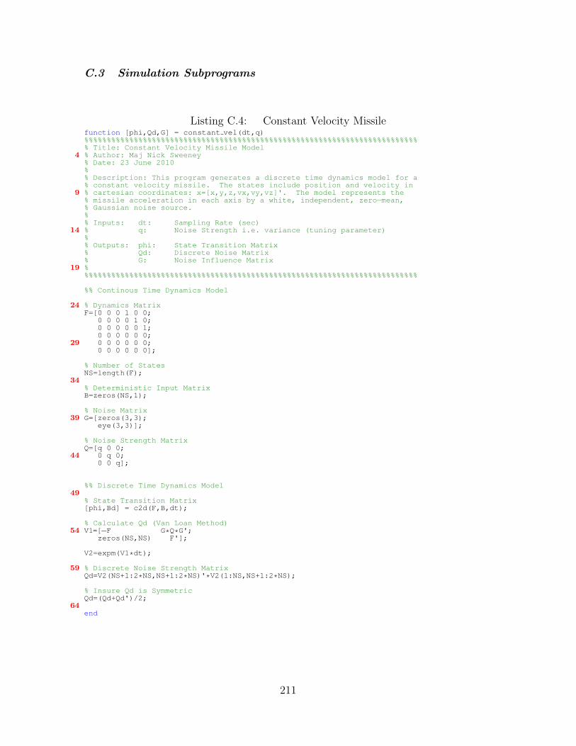
C.3 Simulation Subprograms

Listing C.4: Constant Velocity Missilefunction [phi,Qd,G] = constant vel(dt,q)%%%%%%%%%%%%%%%%%%%%%%%%%%%%%%%%%%%%%%%%%%%%%%%%%%%%%%%%%%%%%%%%%%%%%%%%%%% Title: Constant Velocity Missile Model

4 % Author: Maj Nick Sweeney% Date: 23 June 2010%% Description: This program generates a discrete time dynamics model for a% constant velocity missile. The states include position and velocity in

9 % cartesian coordinates: x=[x,y,z,vx,vy,vz]'. The model represents the% missile acceleration in each axis by a white, independent, zero−mean,% Gaussian noise source.%% Inputs: dt: Sampling Rate (sec)

14 % q: Noise Strength i.e. variance (tuning parameter)%% Outputs: phi: State Transition Matrix% Qd: Discrete Noise Matrix% G: Noise Influence Matrix

19 %%%%%%%%%%%%%%%%%%%%%%%%%%%%%%%%%%%%%%%%%%%%%%%%%%%%%%%%%%%%%%%%%%%%%%%%%%%

%% Continous Time Dynamics Model

24 % Dynamics MatrixF=[0 0 0 1 0 0;

0 0 0 0 1 0;0 0 0 0 0 1;0 0 0 0 0 0;

29 0 0 0 0 0 0;0 0 0 0 0 0];

% Number of StatesNS=length(F);

34% Deterministic Input MatrixB=zeros(NS,1);

% Noise Matrix39 G=[zeros(3,3);

eye(3,3)];

% Noise Strength MatrixQ=[q 0 0;

44 0 q 0;0 0 q];

%% Discrete Time Dynamics Model49

% State Transition Matrix[phi,Bd] = c2d(F,B,dt);

% Calculate Qd (Van Loan Method)54 V1=[−F G*Q*G';

zeros(NS,NS) F'];

V2=expm(V1*dt);

59 % Discrete Noise Strength MatrixQd=V2(NS+1:2*NS,NS+1:2*NS)'*V2(1:NS,NS+1:2*NS);

% Insure Qd is SymmetricQd=(Qd+Qd')/2;

64end

211

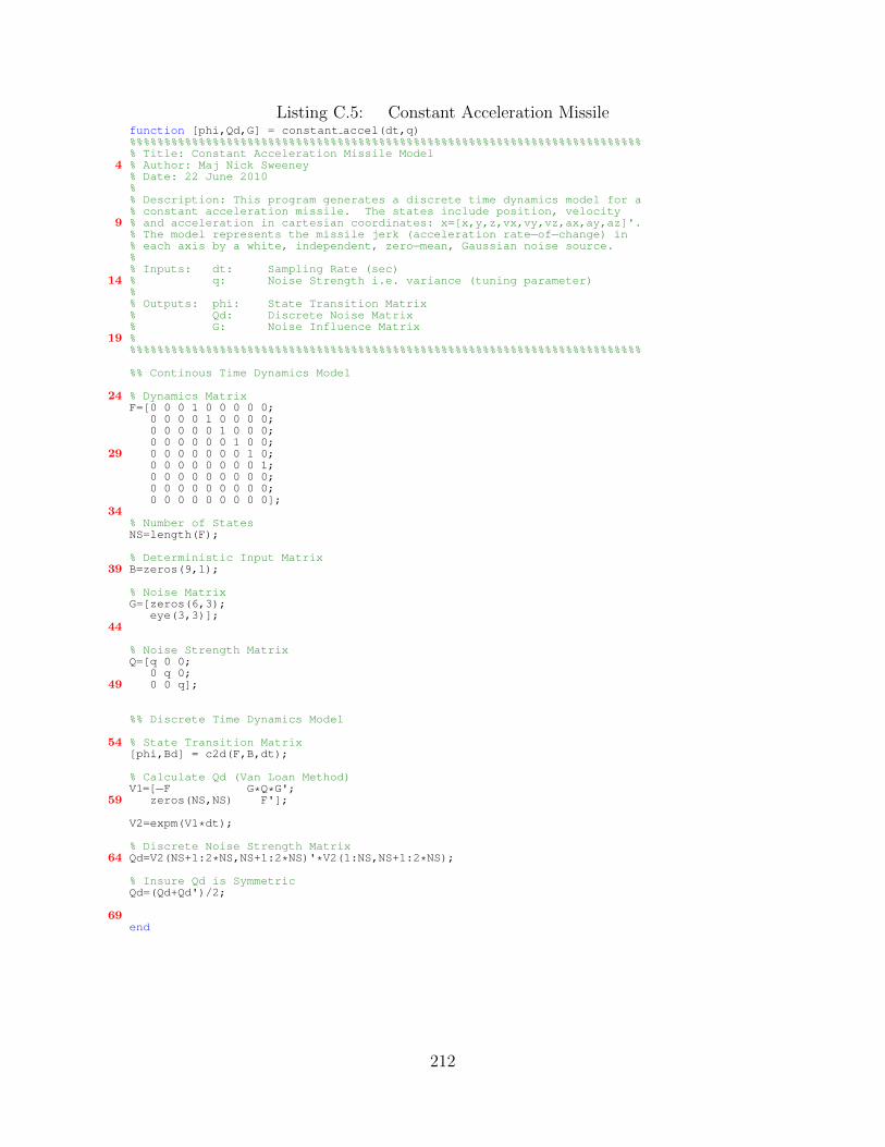
Listing C.5: Constant Acceleration Missilefunction [phi,Qd,G] = constant accel(dt,q)%%%%%%%%%%%%%%%%%%%%%%%%%%%%%%%%%%%%%%%%%%%%%%%%%%%%%%%%%%%%%%%%%%%%%%%%%%% Title: Constant Acceleration Missile Model

4 % Author: Maj Nick Sweeney% Date: 22 June 2010%% Description: This program generates a discrete time dynamics model for a% constant acceleration missile. The states include position, velocity

9 % and acceleration in cartesian coordinates: x=[x,y,z,vx,vy,vz,ax,ay,az]'.% The model represents the missile jerk (acceleration rate−of−change) in% each axis by a white, independent, zero−mean, Gaussian noise source.%% Inputs: dt: Sampling Rate (sec)

14 % q: Noise Strength i.e. variance (tuning parameter)%% Outputs: phi: State Transition Matrix% Qd: Discrete Noise Matrix% G: Noise Influence Matrix

19 %%%%%%%%%%%%%%%%%%%%%%%%%%%%%%%%%%%%%%%%%%%%%%%%%%%%%%%%%%%%%%%%%%%%%%%%%%%


24 % Dynamics MatrixF=[0 0 0 1 0 0 0 0 0;

0 0 0 0 1 0 0 0 0;0 0 0 0 0 1 0 0 0;0 0 0 0 0 0 1 0 0;

29 0 0 0 0 0 0 0 1 0;0 0 0 0 0 0 0 0 1;0 0 0 0 0 0 0 0 0;0 0 0 0 0 0 0 0 0;0 0 0 0 0 0 0 0 0];

34% Number of StatesNS=length(F);

% Deterministic Input Matrix39 B=zeros(9,1);

% Noise MatrixG=[zeros(6,3);

eye(3,3)];44


0 q 0;49 0 0 q];

%% Discrete Time Dynamics Model

54 % State Transition Matrix[phi,Bd] = c2d(F,B,dt);

% Calculate Qd (Van Loan Method)V1=[−F G*Q*G';

59 zeros(NS,NS) F'];

V2=expm(V1*dt);

% Discrete Noise Strength Matrix64 Qd=V2(NS+1:2*NS,NS+1:2*NS)'*V2(1:NS,NS+1:2*NS);

% Insure Qd is SymmetricQd=(Qd+Qd')/2;

69end

212

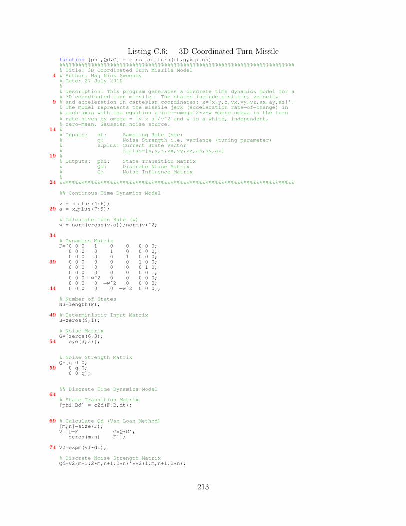
Listing C.6: 3D Coordinated Turn Missilefunction [phi,Qd,G] = constant turn(dt,q,x plus)%%%%%%%%%%%%%%%%%%%%%%%%%%%%%%%%%%%%%%%%%%%%%%%%%%%%%%%%%%%%%%%%%%%%%%%%%%% Title: 3D Coordinated Turn Missile Model

4 % Author: Maj Nick Sweeney% Date: 27 July 2010%% Description: This program generates a discrete time dynamics model for a% 3D coordinated turn missile. The states include position, velocity

9 % and acceleration in cartesian coordinates: x=[x,y,z,vx,vy,vz,ax,ay,az]'.% The model represents the missile jerk (acceleration rate−of−change) in% each axis with the equation a dot=−omegaˆ2*v+w where omega is the turn% rate given by omega = |v x a |/vˆ2 and w is a white, independent,% zero−mean, Gaussian noise source.

14 %% Inputs: dt: Sampling Rate (sec)% q: Noise Strength i.e. variance (tuning parameter)% x plus: Current State Vector% x plus=[x,y,z,vx,vy,vz,ax,ay,az]

19 %% Outputs: phi: State Transition Matrix% Qd: Discrete Noise Matrix% G: Noise Influence Matrix%

24 %%%%%%%%%%%%%%%%%%%%%%%%%%%%%%%%%%%%%%%%%%%%%%%%%%%%%%%%%%%%%%%%%%%%%%%%%%


v = x plus(4:6);29 a = x plus(7:9);

% Calculate Turn Rate (w)w = norm(cross(v,a))/norm(v)ˆ2;

34% Dynamics MatrixF=[0 0 0 1 0 0 0 0 0;

0 0 0 0 1 0 0 0 0;0 0 0 0 0 1 0 0 0;

39 0 0 0 0 0 0 1 0 0;0 0 0 0 0 0 0 1 0;0 0 0 0 0 0 0 0 1;0 0 0 −wˆ2 0 0 0 0 0;0 0 0 0 −wˆ2 0 0 0 0;

44 0 0 0 0 0 −wˆ2 0 0 0];

% Number of StatesNS=length(F);

49 % Deterministic Input MatrixB=zeros(9,1);

% Noise MatrixG=[zeros(6,3);

54 eye(3,3)];


59 0 q 0;0 0 q];

%% Discrete Time Dynamics Model64

% State Transition Matrix[phi,Bd] = c2d(F,B,dt);

69 % Calculate Qd (Van Loan Method)[m,n]=size(F);V1=[−F G*Q*G';

zeros(m,n) F'];

74 V2=expm(V1*dt);

% Discrete Noise Strength MatrixQd=V2(m+1:2*m,n+1:2*n)'*V2(1:m,n+1:2*n);

213

79 % Insure Qd is SymmetricQd=(Qd+Qd')/2;

end

214

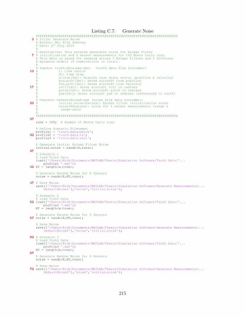
Listing C.7: Generate Noise%%%%%%%%%%%%%%%%%%%%%%%%%%%%%%%%%%%%%%%%%%%%%%%%%%%%%%%%%%%%%%%%%%%%%%%%%%

2 % Title: Generate Noise% Author: Maj Nick Sweeney% Date: 27 July 2010%% Description: This program generates noise for Kalman Filter

7 % initialization and 4 sensor measurements for 100 Monte Carlo runs.% This data is saved for seeding across 3 Kalman Filters and 3 different% dynamics models (9 combinations in total).%% Inputs: truth data xxx.mat: (truth data file includes:)

12 % t: time vector% dt: time step% x true(6xt): missile true state vector (position & velocity)% pos acft(3xt): drone aircraft true position% vel acft(3xt): drone aircraft true velocity

17 % roll(1xt): drone aircraft roll in radians% pitch(1xt): drone aircraft pitch in radians% yaw(1xt); drone aircraft yaw in radians (referenced to north)%% Outputs: DefaultNoiseX.mat (noise file data includes:)

22 % initial noise(6xruns): Kalman filter initialization noise% noise(8xtxruns): noise for 4 sensor measurements (range &% range−rate)%%%%%%%%%%%%%%%%%%%%%%%%%%%%%%%%%%%%%%%%%%%%%%%%%%%%%%%%%%%%%%%%%%%%%%%%%%%

27runs = 100; % Number of Monte Carlo runs

% Define Scenario Filenamesprofile1 = 'truth data below';

32 profile2 = 'truth data ts';profile3 = 'truth data vert';

% Generate Initial Kalman Filter Noiseinitial noise = randn(6,runs);

37% Scenario 1% Load Truth Dataload(['/Users/Nick/Documents/MATLAB/Thesis/Simulation Software/Truth Data/'...

profile1 '.mat'])42 NT = length(x true);

% Generate Random Noise for 4 Sensorsnoise = randn(8,NT,runs);

47 % Save Noisesave(['/Users/Nick/Documents/MATLAB/Thesis/Simulation Software/Generate Measurements/...

DefaultNoise1'],'noise','initial noise');

% Scenario 2% Load Truth Data

52 load(['/Users/Nick/Documents/MATLAB/Thesis/Simulation Software/Truth Data/'...profile2 '.mat'])

NT = length(x true);

% Generate Random Noise for 4 Sensors57 noise = randn(8,NT,runs);

% Save Noisesave(['/Users/Nick/Documents/MATLAB/Thesis/Simulation Software/Generate Measurements/...


62 % Scenario 3% Load Truth Dataload(['/Users/Nick/Documents/MATLAB/Thesis/Simulation Software/Truth Data/'...

profile3 '.mat'])NT = length(x true);

67% Generate Random Noise for 4 Sensorsnoise = randn(8,NT,runs);

% Save Noise72 save(['/Users/Nick/Documents/MATLAB/Thesis/Simulation Software/Generate Measurements/...


215

Listing C.8: Generate Measurementsfunction [z1,z2,z3,z4,z5,z6,z7,detect] = gen meas seed(x true,pos acft,vel acft,roll,...

pitch,yaw,noise)%%%%%%%%%%%%%%%%%%%%%%%%%%%%%%%%%%%%%%%%%%%%%%%%%%%%%%%%%%%%%%%%%%%%%%%%%%

3 % Title: Generate Measurements% Author: Maj Nick Sweeney% Date: 27 July 2010%% Description: This program generates noise corrupted measurements of

8 % missile distance and velocity using seven sensors located on an% aircraft. It also produces a random number of clutter measurements.%% Inputs: x true: 6x1 true state vector for missile% pos acft: 3x1 true position vector for drone aircraft

13 % vel acft: 3x1 true velocity vector for drone aircraft% roll: current roll of aircraft in radians% pitch: current pitch of aircraft in radians% yaw: current yaw (referenced to north) of acft in radians%

18 % Outputs: detect: 7x1 vector indicating which sensors observed a target% z1−z7: 2xN vector of sensor range and range−rate measurments%% Note: Inputs are all in local−level Earth−centered navigation frame%%%%%%%%%%%%%%%%%%%%%%%%%%%%%%%%%%%%%%%%%%%%%%%%%%%%%%%%%%%%%%%%%%%%%%%%%%

23% Define Sensor Locations (meters)% Sensor 1 − Aircraft Nose (top)px1 = 8;py1 = 0;

28 pz1 = −0.5;% Sensor 2 − Aircraft Nose (bottom)px2 = 8;py2 = 0;pz2 = 0.5;

33 % Sensor 3 − Aircraft Left Wing (top)px3 = 0;py3 = −5;pz3 = 0;% Sensor 4 − Aircraft Left Wing (bottom)

38 px4 = 0;py4 = −5;pz4 = 0.1;% Sensor 5 − Aircraft Right Wing (top)px5 = 0;

43 py5 = 5;pz5 = 0;% Sensor 6 − Aircraft Right Wing (bottom)px6 = 0;py6 = 5;

48 pz6 = 0.1;% Sensor 7 − Aircraft Tail (omni−directional)px7 = −8;py7 = 0;pz7 = −1;

53% Convert Missile LL Nav Earth−centered Coordinates to Body Frame% Nav to Body RotationC1 = [cos(yaw) sin(yaw) 0; % rotation about z−axis

−sin(yaw) cos(yaw) 0;58 0 0 1];

C2 = [cos(pitch) 0 −sin(pitch); % rotation about y−axis0 1 0;sin(pitch) 0 cos(pitch)];

63C3 = [1 0 0; % rotation about x−axis

0 cos(roll) sin(roll);0 −sin(roll) cos(roll)];

68 Cnb = C3*C2*C1;

% Missile True Position in Body Framepos true b = Cnb*(x true(1:3)−pos acft);

73 % Missile True Velocity in Body Framevel true b = Cnb*(x true(4:6)−vel acft);

% Define Position and Velocity Variables

216

x = pos true b(1);78 y = pos true b(2);

z = pos true b(3);vx = vel true b(1);vy = vel true b(2);vz = vel true b(3);

83% Define Sensor Noise% Sensor Range Accuracy is Better than 2.5% of Range (used 2.5% for 2 sigma)sigma dist = 0.025/2;% Sensor Velocity Accuracy is Better than 0.25 km/hr (used 0.25 m/s for 2 sigma)

88 sigma vel = 0.25/2;

% Randomly Determine Number of Clutter Measurements on each SensorNC = randi(3,4,1); % generates 1−3 ghost targets with equal probability

93 if z>0 % missile is below aircraft

detect = [0; 1; 0; 1; 0; 1; 1];

% Sensors 1,3,5 (no measurements)98 z1 = [];

z3 = [];z5 = [];

% Sensor 2103 % True Measurements

dist = sqrt((x−px2)ˆ2+(y−py2)ˆ2+(z−pz2)ˆ2);speed = −(vx*(x−px2)+vy*(y−py2)+vz*(z−pz2))/dist;z2(1,1) = dist+sigma dist*dist*noise(1);z2(2,1) = speed+sigma vel*noise(2);

108 % Clutter Measurements (uniformly distributed)z2(1,2:NC(1)+1) = 350*rand(1,NC(1));z2(2,2:NC(1)+1) = 650*rand(1,NC(1));










else % missile is above aircraft143

detect = [1; 0; 1; 0; 1; 0; 1];

% Sensors 2,4,6 (no measurements)z2 = [];

148 z4 = [];z6 = [];

% Sensor 1% True Measurements

153 dist = sqrt((x−px1)ˆ2+(y−py1)ˆ2+(z−pz1)ˆ2);speed = −(vx*(x−px1)+vy*(y−py1)+vz*(z−pz1))/dist;

217

z1(1,1) = dist+sigma dist*dist*noise(1);z1(2,1) = speed+sigma vel*noise(2);% Clutter Measurements (uniformly distributed)

158 z1(1,2:NC(1)+1) = 350*rand(1,NC(1));z1(2,2:NC(1)+1) = 650*rand(1,NC(1));


163 dist = sqrt((x−px3)ˆ2+(y−py3)ˆ2+(z−pz3)ˆ2);speed = −(vx*(x−px3)+vy*(y−py3)+vz*(z−pz3))/dist;z3(1,1) = dist+sigma dist*dist*noise(3);z3(2,1) = speed+sigma vel*noise(4);% Clutter Measurements (uniformly distributed)








end

193 end

218

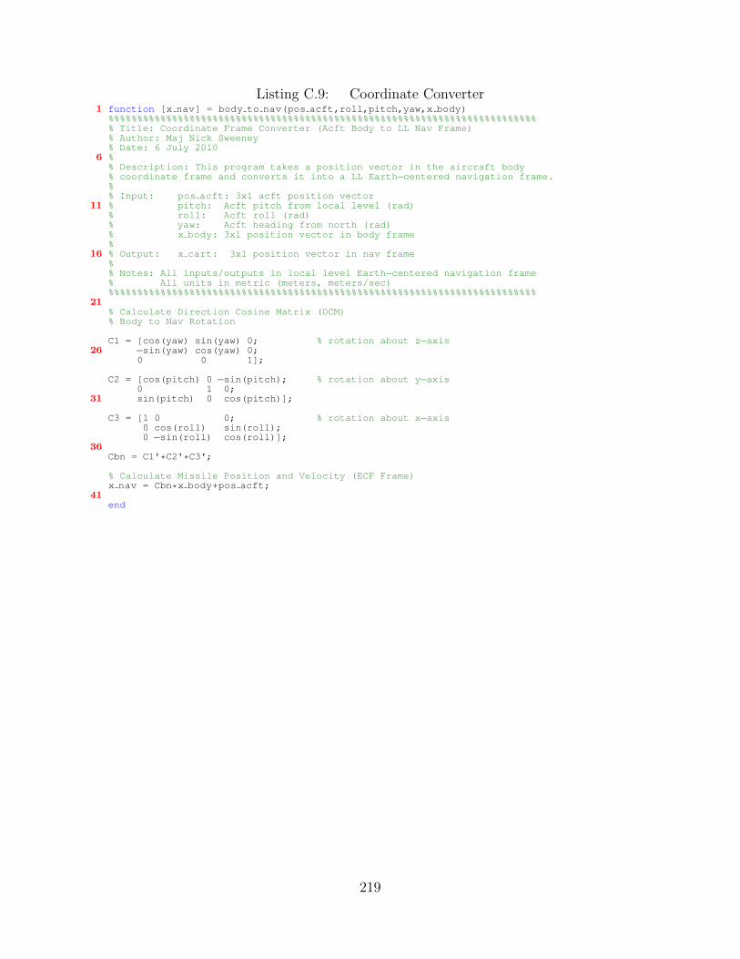
Listing C.9: Coordinate Converter1 function [x nav] = body to nav(pos acft,roll,pitch,yaw,x body)

%%%%%%%%%%%%%%%%%%%%%%%%%%%%%%%%%%%%%%%%%%%%%%%%%%%%%%%%%%%%%%%%%%%%%%%%%%% Title: Coordinate Frame Converter (Acft Body to LL Nav Frame)% Author: Maj Nick Sweeney% Date: 6 July 2010

6 %% Description: This program takes a position vector in the aircraft body% coordinate frame and converts it into a LL Earth−centered navigation frame.%% Input: pos acft: 3x1 acft position vector

11 % pitch: Acft pitch from local level (rad)% roll: Acft roll (rad)% yaw: Acft heading from north (rad)% x body: 3x1 position vector in body frame%

16 % Output: x cart: 3x1 position vector in nav frame%% Notes: All inputs/outputs in local level Earth−centered navigation frame% All units in metric (meters, meters/sec)%%%%%%%%%%%%%%%%%%%%%%%%%%%%%%%%%%%%%%%%%%%%%%%%%%%%%%%%%%%%%%%%%%%%%%%%%%

21% Calculate Direction Cosine Matrix (DCM)% Body to Nav Rotation

C1 = [cos(yaw) sin(yaw) 0; % rotation about z−axis26 −sin(yaw) cos(yaw) 0;

0 0 1];

C2 = [cos(pitch) 0 −sin(pitch); % rotation about y−axis0 1 0;

31 sin(pitch) 0 cos(pitch)];

C3 = [1 0 0; % rotation about x−axis0 cos(roll) sin(roll);0 −sin(roll) cos(roll)];

36Cbn = C1'*C2'*C3';

% Calculate Missile Position and Velocity (ECF Frame)x nav = Cbn*x body+pos acft;

41end

219

Listing C.10: Nonlinear Transform Functionfunction [ZSigma] = h transform(XSigma,p n,v n)

2 %%%%%%%%%%%%%%%%%%%%%%%%%%%%%%%%%%%%%%%%%%%%%%%%%%%%%%%%%%%%%%%%%%%%%%%%%%% Title: Nonlinear Distance Function% Author: Maj Nick Sweeney% Date: 5 August 2010%

7 % Description: This program takes a set of sigma points from an unscented% Kalman filter or a set of particles from a particle filter and transforms% them through a nonlinear observation function.%% Inputs: XSimga: UKF Sigma Points or PF Particles

12 % p n: Sensor Position in Earth−centered LL Nav Frame% v n: Sensor Velocity in Earth−centered LL Nav Frame%% Outputs: ZSigma: Sigma Points or Particles Transformed through% Distance and Velocity Functions

17 %%%%%%%%%%%%%%%%%%%%%%%%%%%%%%%%%%%%%%%%%%%%%%%%%%%%%%%%%%%%%%%%%%%%%%%%%%%

N = length(XSigma);p matrix = p n*ones(1,N);

22 v matrix = v n*ones(1,N);

% Distance TransformZSigma(1,:) = sqrt((XSigma(1,:)−p matrix(1,:)).ˆ2+(XSigma(2,:)−p matrix(2,:)).ˆ2+(...

XSigma(3,:)−p matrix(3,:)).ˆ2);

27 % Velocity TransformZSigma(2,:) = −((XSigma(4,:)−v matrix(1,:)).*(XSigma(1,:)−p matrix(1,:))+(XSigma(5,:)−...

v matrix(2,:)).*(XSigma(2,:)−p matrix(2,:))+(XSigma(6,:)−v matrix(3,:)).*(XSigma...(3,:)−p matrix(3,:)))./ZSigma(1,:);

end

220

Bibliography

1. 412th Operational Support Squadron. Air Force Flight Test Center Instruction11-1, January 2004.

2. 412th Range Squadron. Glite System Version 3, January 2011.

3. Barton, David A. Paired Layering: The Argo Way of Simulation Construction.National Air and Space Intelligence Center, December 2005.

4. Blackman, Samuel. “Multiple Hypothesis Tracking for Multiple Target Tracking”.IEEE Aerospace and Electronic Systems Magazine, 19:5–18, 2004.

5. Blackman, Samuel and Robert Popoli. Modern Tracking Systems. Artech House,1999.

6. Bradley, Joseph. Miss Distance Vector Scoring System. United States PatentNumber 5614910, 1997.

7. Brown, Robert G. and Patrick Y. C. Hwang. Introduction to Random Signals andApplied Kalman Filtering. John Wiley and Sons, 3rd edition, 1997.

8. DiFilippo, David and Lori Campbell. “Design and Implementation of a TrackingAlgorithm for Active Missile Approach Warning Systems”. Canadian Conf. onElectrical and Computer Engineering, volume 2, 756–759. 1995.

9. Farrell, William. “Interacting multiple model filter for tactical ballistic missiletracking”. IEEE Transactions on Aerospace and Electronic Systems, volume 44,418–426. 2008.

10. Folster, Florian, Hermann Rohling, and Urs Lubbert. “An Automotive RadarNetwork Based on 77GHz FMCW Sensors”. IEEE Int. Radar Conf. 2005.

11. Incorporated, Hebco. USAF Series C-12C/D Technical Order 1C-12A-1, October2010.

12. Kalandros, Michael K., Lidija Trailovic, Lucy Y. Pao, and Yaakov Bar-Shalom.“Tutorial on Multisensor Management and Fusion Algorithms for Target Track-ing”. American Control Conf. 2004.

13. Kikic, Goran and Branko Kovacevic. “Target Tracking with Passive IR sensors”.Int. Conf. on Telecommunications in Modern Satellite, Cable and BroadcastingService, volume 2, 745–748. 2001.

14. Kim, Brian. Evaluating the Correlation Characteristics of Arbitrary AM and FMRadio Signals for the Purpose of Navigation. Master’s thesis, Air Force Instituteof Technology, 2006.

15. Klotz, Michael. An Automotive Short Range High Resolution Pulse Radar Net-work. Ph.D. thesis, Technische Univ. Hamburg-Hamburg, 2002.

221

16. Mahmood, Sultan, Jane Colee, Jim Luse, Dwight Payne, Joseph Taylor, andSamuel Burkett. “Gulf Range Target Control Using Rajpo GPS Equipment, TestResults and an Alternate Concept”. Position Location and Navigation Sympo-sium, 306–313. 1992.

17. Maybeck, Peter, James Negro, Salvatore Cusumano, and Manuel De Ponte. “ANew Tracker for Air-to-Air Missile Targets”. IEEE Transactions on AutomaticControl, 900–905. 1979.

18. Maybeck, Peter S. Stochastic Models, Estimation and Control, volume 1. NavtechBook and Software Store, 1994.

19. Maybeck, Peter S. Stochastic Models, Estimation and Control, volume 2. NavtechBook and Software Store, 1994.

20. van der Merwe, Rudolph, Arnaud Doucet, Nando de Freitas, and Eric Wan. TheUnscented Particle Filter. Technical report, Cambridge University EngineeringDepartment, 2000.

21. Miah, M. Suruz and Wail Gueaieb. “A Stochastic Approach of Mobil RobotNavigation Using Customized RFID Systems”. Int. Conf. on Signals, Circuitsand Systems. 2009.

22. Minor, Roy and David Rowe. “Utilization of GPS/MEMS-IMU for Measurementof Dynamics for Range Testing of Missiles and Rockets”. IEEE Position Locationand Navigation Symposium, 602-607. 1998.

23. Minvielle, Pierre. “Decades of improvements in re-entry ballistic vehicle tracking”.IEEE Aerospace and Electronic Systems Magazine, 20:1–14, 2005.

24. Misra, Pratap and Per Enge. Global Positioning System Signals, Measurementsand Performance. Ganga-Jamuna Press, 2nd edition, 2006.

25. Musick, Stanton H. User’s Guide for Profgen, A Trajectory Generator. Air ForceResearch Laboratory, December 2004.

26. Pastorelli, A., G. Torricelli, M. Scabia, E. Biagi, and L. Masotti. “A Real-Time2-D Vector Doppler System for Clinical Experimentation”. IEEE Transactionson Medical Imaging, 27:1515–1524, 2008.

27. Pastorelli, A., G. Torricelli, M. Scabia, E. Biagi, and L. Masotti. “A Real-Time2-D Vector Doppler System for Clinical Experimentation”. IEEE Transactionson Medical Imaging, volume 27, 1515–1524. 2008.

28. Qureshi, W.A., R.A.J. Khan, M. Ahmed, and A. Bashir. “An Efficient Approachfor Target Tracking and Error Minimization by Kalman Filtering Technique”. Int.Conf. on Electrical Engineering, 1–6. 2007.

29. Rohling, Hermann and Marc-Michael Meinecke. “Waveform Design Principles forAutomotive Radar Systems”. CIE Int. Radar Conf. 2001.

222

30. Rohling, Hermann and Christof Moller. “Radar Waveform for Automotive RadarSystems and Applications”. IEEE Radar Conf. 2008.

31. Siouris, George, Guanrong Chen, and Jianrong Wang. “Tracking an IncomingBallistic Missile Using an Extended Interval Kalman Filter”. IEEE Transactionson Aerospace and Electronic Systems. 1997.

32. Smart Microwave Sensors. Universal Medium Range Radar Documentation, May2010.

33. Stadnik, P.J. “Flight test of an Integrated Digital GPS Translator”. IEEE Posi-tion Location and Navigation Symposium, 75-82. 1996.

34. Steel, Robin and Peter Fish. “Error Propagation Bounds in Dual and Triple BeamVector Doppler Ultrasound”. IEEE Transactions on Ultrasonics, Ferroelectrics,and Frequency Control, volume 49, 1222–1230. 2002.

35. Steel, Robin and Peter J. Fish. “Error Propagation Bounds in Dual and TripleBeam Vector Doppler Ultrasound”. IEEE Transactions on Ultrasonics, 49:1222–1230, 2002.

36. Sweeney, Nicholas and Kenneth Fisher. “Air-to-Air Missile Vector Scoring”. IEEEInt. Conf. on Control Applications, 579–586. 2011.

37. Tafti, Abdolreza and Nasser Sadati. “A Hybrid Fuzzy Dynamic Model for Ma-neuvering Targets”. IEEE Aerospace Conf., 1–6. 2009.

38. Thompson, T. “Demonstration of a Precision Missile Intercept MeasurementTechnique”. John Hopkins APL Technical Digest, 19:513–23, 1998.

39. Titterton, David H. and John L. Weston. Strapdown Inertial Navigation Tech-nology. The Institution of Electrical Engineers, 2nd edition, 2004.

40. Tu, Po-Jen and Jean-Fu Kiang. “Estimation on Location, Velocity, and Accel-eration with High Precision for Collision Avoidance”. IEEE Transactions onIntelligent Transportation Systems, volume 2, 374–379. 2010.

41. Veth, Michael. Fusion of Imaging and Inertial Sensors for Navigation. Ph.D.thesis, Air Force Institute of Technology, September 2006.

42. Xu, Jian-Zhong, Zu-Lin Wang, Yi-Huan Zhao, and Xu-Jing Guo. “A DistanceEstimation Algorithm Based on Infrared Imaging Guided”. Int. Conf. on MachineLearning and Cybernetics, volume 4, 2343–2346. 2009.

223

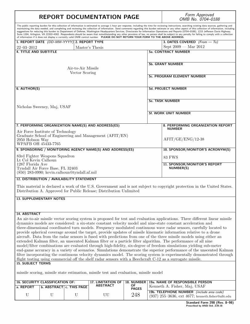
REPORT DOCUMENTATION PAGE Form ApprovedOMB No. 0704–0188

The public reporting burden for this collection of information is estimated to average 1 hour per response, including the time for reviewing instructions, searching existing data sources, gathering andmaintaining the data needed, and completing and reviewing the collection of information. Send comments regarding this burden estimate or any other aspect of this collection of information, includingsuggestions for reducing this burden to Department of Defense, Washington Headquarters Services, Directorate for Information Operations and Reports (0704–0188), 1215 Jefferson Davis Highway,Suite 1204, Arlington, VA 22202–4302. Respondents should be aware that notwithstanding any other provision of law, no person shall be subject to any penalty for failing to comply with a collectionof information if it does not display a currently valid OMB control number. PLEASE DO NOT RETURN YOUR FORM TO THE ABOVE ADDRESS.

1. REPORT DATE (DD–MM–YYYY) 2. REPORT TYPE 3. DATES COVERED (From — To)

4. TITLE AND SUBTITLE 5a. CONTRACT NUMBER

5b. GRANT NUMBER

5c. PROGRAM ELEMENT NUMBER

5d. PROJECT NUMBER

5e. TASK NUMBER

5f. WORK UNIT NUMBER

6. AUTHOR(S)

7. PERFORMING ORGANIZATION NAME(S) AND ADDRESS(ES) 8. PERFORMING ORGANIZATION REPORTNUMBER

9. SPONSORING / MONITORING AGENCY NAME(S) AND ADDRESS(ES) 10. SPONSOR/MONITOR’S ACRONYM(S)

11. SPONSOR/MONITOR’S REPORTNUMBER(S)

12. DISTRIBUTION / AVAILABILITY STATEMENT

13. SUPPLEMENTARY NOTES

14. ABSTRACT

15. SUBJECT TERMS

16. SECURITY CLASSIFICATION OF:

a. REPORT b. ABSTRACT c. THIS PAGE

17. LIMITATION OFABSTRACT

18. NUMBEROFPAGES

19a. NAME OF RESPONSIBLE PERSON

19b. TELEPHONE NUMBER (include area code)

Standard Form 298 (Rev. 8–98)Prescribed by ANSI Std. Z39.18

22–03–2012 Master’s Thesis Sept 2009 — Mar 2012


Nicholas Sweeney, Maj, USAF

Air Force Institute of TechnologyGraduate School of Engineering and Management (AFIT/EN)2950 Hobson WayWPAFB OH 45433-7765

AFIT/GE/ENG/12-38

83rd Fighter Weapons SquadronLt Col Kevin Calhoun1287 Florida AveTyndall Air Force Base, FL 32403(850) 283-0990; [email protected]

83 FWS

This material is declared a work of the U.S. Government and is not subject to copyright protection in the United States.Distribution A. Approved for Public Release; Distribution Unlimited

An air-to-air missile vector scoring system is proposed for test and evaluation applications. Three different linear missiledynamics models are considered: a six-state constant velocity model and nine-state constant acceleration andthree-dimensional coordinated turn models. Frequency modulated continuous wave radar sensors, carefully located toprovide spherical coverage around the target, provide updates of missile kinematic information relative to a droneaircraft. Data from the radar sensors is fused with predictions from one of the three missile models using either anextended Kalman filter, an unscented Kalman filter or a particle filter algorithm. The performance of all ninemodel/filter combinations are evaluated through high-fidelity, six-degree of freedom simulations yielding sub-meterend-game accuracy in a variety of scenarios. Simulations demonstrate the superior performance of the unscented Kalmanfilter incorporating the continuous velocity dynamics model. The scoring system is experimentally demonstrated throughflight testing using commercial off the shelf radar sensors with a Beechcraft C-12 as a surrogate missile.

missile scoring, missile state estimation, missile test and evaluation, missile model

U U U UU 248

Kenneth A. Fisher, Maj, USAF

(937) 255–3636, ext 4677; [email protected]