AIAA 99-0122 A Solution on the F-18C for Store Separation

AIAA 99-0122A Solution on the F-18C for Store SeparationSimulation Using Cobalt60R. F. Tomaro, F. C. Witzeman and W. Z. StrangComputational Sciences BranchAir Vehicles DirectorateAir Force Research LaboratoryWright-Patterson AFB, OH

1American Institute of Aeronautics and Astronautics

A SOLUTION ON THE F-18C FOR STORE SEPARATION SIMULATION USING Cobalt60

Robert F. Tomaro*, Frank C. Witzeman* and William Z. Strang*

Air Force Research LaboratoryAir Vehicles Directorate

WPAFB Ohio 45433

Abstract

A demonstration is presented of the ability ofComputational Fluid Dynamics (CFD) methods topredict store carriage loads and support store trajectorygeneration. A complete, complex aircraft, the F/A-18C, was modeled with actual stores in their carriagepositions. Cobalt60, a parallel, implicit unstructuredflow solver was used to calculate the flow field andresultant aerodynamic loads on grids composed oftetrahedral cells. Three grids were used to simulatethree different flow field approximations. The firstgrid was a purely inviscid grid containing 3.15 millioncells. The second grid was made up of 3.96 millioncells clustered to capture viscous effects on only thestore components. The third grid was a full viscousgrid containing 6.62 million cells. Store carriage loadsfor two flight conditions were calculated and comparedwith wind-tunnel measurements and flight-test data foreach of the above grids. The resulting carriage loadswere used in a separate six degree-of-freedom (6DOF)rigid-body motion code to generate store trajectories.All CFD solutions were second-order accurate and runto steady-state with CFL numbers of one million.Turnaround times ranged from 6 to 21 hours,depending on the number of processors used.

Introduction

The incorporation of CFD tools into the storecertification process is limited at the present.Accurate, reliable answers must be provided quicklyand economically. First, the entire solution processmust be accomplished in a matter of days. With thematuring of the unstructured grid generation process,full viscous grids can be generated in under a week’s

time on very complex configurations. Using massivelyparallel supercomputers and convergence accelerationtechniques, turbulent solution CPU times onunstructured grids have been reduced to a number ofhours. Unstructured grids also have the inherentability to be decomposed into equal or nearly equalsubsections. This quality translates into perfect or nearperfect load balance allowing the efficient use ofmassively parallel supercomputers.

The Air Force SEEK EAGLE ACFD (AppliedComputational Fluid Dynamics) project wants toprovide the store separation engineer with accurate,reliable and efficient CFD tools. From a CFDdeveloper’s point of view, capturing the fluid physicsand resulting aerodynamics accurately with quickturnaround time is the goal. For store integration andcertification, obtaining accurate carriage loads in atimely manner is very important. If this isaccomplished, then CFD has demonstrated one of itsrelative contributions. Trajectory generation/analysis,ejector modeling, etc. are separate technology areaswhich are best addressed by store certification experts.

Past demonstrative efforts have used severalcombinations of grid and flow solver techniques.Accurate predictions of store carriage loads on ageneric wing/pylon/finned-store configuration1-5 werepresented in 1992. These results were mostly Eulercalculations on a “simple” geometry. In 1996, a morecomplex aircraft/store configuration was studied, the F-16/generic finned-store6-8. However, questions aboutthe accuracy of the wind-tunnel measurements wereraised in that study. In addition, incorporating CFDtools into the certification process has been slowed by alack of validations and demonstrations on “real”configurations.

The F/A-18C JDAM configuration was chosen forthis study because both wind-tunnel measurements andflight-test data exist. For the flight test, bothphotogrametrics and telemetry were used to track the

* Aerospace Engineer, Computational Sciences BranchThis paper is declared a work of the U.S. Government and isnot subject to copyright protection in the United States.


flight path of the released JDAM. The wind-tunneltest used a six-percent scale F/A-18C model. Both aCaptive Trajectory System (CTS) and a pylon mountedJDAM approach were used in the wind tunnel. TheCTS and carriage wind-tunnel measurementscorrelated well with each other at only a few selectconditions9. JDAM trajectories generated from thesedata were compared with flight-test values, and aninverse approach was used to determine the actualcarriage loads which matched flight-test trajectories9.

This document describes the JDAM aerodynamicloads and trajectory results obtained using the AirForce Research Laboratory (AFRL) Cobalt60 flowsolver and the Naval Air Warfare Center (NAWC)NAVSEP trajectory generator. Overviews of eachmethod are provided in the following sections, andflowfield and trajectory results at two Mach numbersare given in the final sections.

Overview of Cobalt60

Cobalt60 is a parallel, implicit unstructured flowsolver developed by the Computational SciencesBranch of the Air Force Research Laboratory10.Godunov’s first-order accurate, exact Riemannmethod11 is the foundation of Cobalt60. Second-orderspatial accuracy, second-order accurate implicit timestepping, viscous terms and turbulence models havebeen added to this procedure. Cobalt60 uses a finite-volume, cell-centered approach. Arbitrary cell types intwo or three dimensions may be used, and a single gridmay be composed of a variety of cell types.Information on the calculation of inviscid and viscousfluxes and the dissipation in Cobalt60 is reported inStrang10. Two one-equation turbulence models havebeen implemented in Cobalt60, the Spalart-Allmaras12

model and the Baldwin-Barth model13.

The implicit algorithm in Cobalt60 wasimplemented and demonstrated by Tomaro14. Theimplicit algorithm resulted in a 5-10 times speed upover the original explicit algorithm with only a ten-percent increase in memory. Inviscid flows wereroutinely obtained with CFL numbers of one million;however, turbulent flows severely limited the CFLnumber. A further modification to the original implicitalgorithm, reported by Strang10, removed the limitationfor viscous flows, allowing CFL numbers of onemillion for most problems. This modified implicitalgorithm resulted in a 7-10 times speed up inconvergence over the original explicit code for viscousflows.

The development of the parallel version ofCobalt60 was reported by Grismer15. Domaindecomposition is the basis for the parallel code. Eachprocessor operates on a subsection (zone) of theoriginal grid. Information is passed betweenprocessors using the Message Passing Interface (MPI)library routines. Cobalt60 has been implemented andtested on IBM SP2’s, Cray T3E’s and SGI Origin2000’s. The resulting speed up of Cobalt60

demonstrated “superscalability” on large cache-basedsystems; i.e., the speed-up factor was greater than thenumber of processors used.

Cobalt60 allows a variety of boundary conditions16.For these F/A-18C simulations, the farfield wasimposed using a modified Riemann invariant method.The surfaces of the body were slip walls for an inviscidsurface or adiabatic no-slip walls for a viscous surface. To account for flow through the engine, a source/sinkpair was utilized. The engine face used a correctedmass flow sink boundary condition to enforce the massflowing out the grid at this boundary surface. Theengine exhaust was modeled with a source boundarycondition to allow flow into the domain from thisboundary surface.

Grid Resolution/Physics Study

Three separate grids were constructed to simulatethe flowfield around the F/A-18C with stores. Thesethree grids were used for a resolution study as well as alevel of physics study. The equation set used in thesimulation impacts the solution time as well as theaerodynamics. Therefore, it is important to knowwhich level of physics is required for an engineeringanalysis. To that end, an inviscid solution, a stores-only viscous solution and a full viscous solution werecalculated and compared. All three grids modeled thecomplete F/A-18C including the inlet duct to theengine face, the boundary layer diverter with flowthrough to the upper surface of the wing, the stair-stepped pylons, and the strakes on the JDAM includingthe notches.

The fully inviscid grid contained 3.15 milliontetrahedral cells. Cobalt60 required approximately 2.4Gb of memory for this case. The grid was generatedusing Gridtool and VGRIDns17, both programsdeveloped by NASA Langley. The F/A-18C wasessentially the first grid attempted with VGRIDns bythe first author. The first step is to construct patchesover the original PLOT3D surfaces. This step requiredapproximately one week. Subsequently, some patches


were further refined. The same surface patching wasused as a basis for all three grids. The second step is toplace sources to control grid spacing and clustering.This is an iterative step until the desired spacing isachieved. Two days were spent on this process. Thethird step is to triangulate the surface patches andproject them to the original PLOT3D surfaces. Thisrequired one day. The final step is to generate thevolume mesh; this step required approximately onehour on an SGI Octane workstation. Figure 1adisplays the inviscid grid around the outboard pylonand JDAM. Notice that the notches in the strakes weremodeled.

The second grid treated the surfaces of the JDAMand fuel tank as viscous surfaces. The rest of theaircraft was simulated with slip walls. This grid wasgenerated using the inviscid surface patching butspecifying the surfaces of the JDAM and fuel tank asviscous surfaces. The second grid contained 3.96million tetrahedral cells with approximately 850,000cells in the boundary layers requiring approximately6.0 Gb of memory for this case. This modification tothe grid required approximately one day. Thegeneration of the volume grid again required one hourof CPU time. Figure 1b shows the viscous grid aroundthe JDAM and the inviscid grid around the outboardpylon. Essentially, the same grid clustering was used.

The full viscous grid contained 6.62 milliontetrahedral cells including approximately 4 millioncells in the boundary layers. This grid was constructedby specifying all surface patches of the inviscid grid asnow being viscous. For the full viscous case, Cobalt60

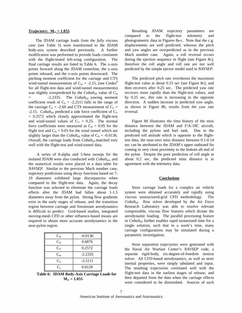
required approximately 10.1 Gb of memory. Ifeverything had proceeded smoothly, this step wouldhave taken a one-day effort. However, the advancingfront in VGRIDns actually kept growing “into” thebody. After consulting with the VGRIDns experts atNASA Langley, it was determined the surface grid mayhave contained some folded triangles and that theclustering of negative volumes in the viscous layerwere the causes (the negative volume cells are removedand then filled with the advancing front method). Toremove these two problems, more sources were addedand strengths modified during a trial and error process.This entire process required about a month of calendartime. The full viscous grid spacing around the JDAMand outboard pylon is shown in Figure 1c. Figures 2aand 2b show the viscous grid clustering at a fuselagestation and a water-line of the aircraft, respectively.

Overview of NAVSEP

Store trajectories may be obtained when carriageloads and isolated store aerodynamics are provided toan independent six-degree-of-freedom, rigid-bodymotion solver. For this F/A-18C JDAM effort, AFRLobtained and used the NAWC NAVSEP trajectorygeneration program18. This code is used routinely bythe Navy, and it requires minimal computer resourcesand user intervention requirements. NAVSEP is basedon the AEDC trajectory generation system19 embeddedin its captive trajectory testing setup. The programintegrates the standard conservation of linear andangular momentum equations for a rigid bodyexperiencing aerodynamic and other body forces andmoments.

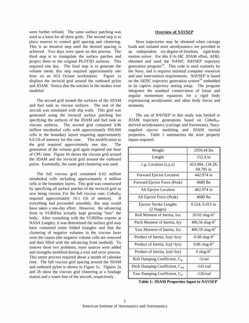
The use of NAVSEP in this study was limited toJDAM trajectory generations based on Cobalt60-derived aerodynamics (carriage and freestream), Navy-supplied ejector modeling and JDAM inertialproperties. Table 1 summarizes the store propertyinputs required.

Weight 2059.44 lbs

Length 152.4 in

c.g. Location (x,y,z) 453.084, 134.28,69.795 in

Forward Ejector Location 442.974 in

Forward Ejector Force (Peak) 4680 lbs

Aft Ejector Location 462.974 in

Aft Ejector Force (Peak) 4680 lbs

Ejector Stroke Lengths (2 Stages)

0.524, 6.015 in

Roll Moment of Inertia, Ixx 20.02 slug-ft2

Pitch Moment of Inertia, Iyy 406.56 slug-ft2

Yaw Moment of Inertia, Izz 406.59 slug-ft2

Product of Inertia, Ixz(=Izx) -0.68 slug-ft2

Product of Inertia, Ixy(=Iyx) 0.86 slug-ft2

Product of Inertia, Iyz(=Izy) 0 slug-ft2

Roll Damping Coefficient, Clp -3/rad

Pitch Damping Coefficient, Cmq -141/rad

Yaw Damping Coefficient, Cnr -126/rad

Table 1: JDAM Properties Input to NAVSEP


In addition to the JDAM aerodynamics and aboveproperties, information related to a decay functionmust be supplied to NAVSEP. This function varieswith lateral and vertical distance of a store with respectto the carriage position such that the carriage loadsdominate the effective aerodynamic forces andmoments at and near the initial release point. Later,the loads decay to the freestream, isolated storeaerodynamics. Typically the vertical separationdistance is much larger than the lateral displacement,and when a store falls anywhere from 7 to 10 bodydiameters away, it is considered to be outside thecarriage influence region.

Results

Two flight conditions were simulated on the threegrids. The first test case was at Mach number M∞ =0.962 with α = 0.46° at an altitude of 6,332 ft. Thesecond flight condition was an altitude of 10,832 ftwith a Mach number M∞ = 1.055 and α = -0.65°. TheSpalart-Allmaras turbulence model was used in theviscous cases. For these simulations, the right side ofthe aircraft was modeled. The x-axis runs aft from thenose to the tail; the y-axis is positive out the rightwing; and the z-axis is positive upward. Since theflight test tracked the JDAM on the left wing, therewill be some sign changes required to match the CFDresults, the wind-tunnel measurements and the flight-test data. The geometric reference quantities used toobtain the aerodynamic coefficients are presented inTable 2.

Reference Area 254.45 in2

Moment ReferenceLength (x-axis)

18.0 in

Moment ReferenceLength (y-axis)

18.0 in

Moment ReferenceLength (z-axis)

18.0 in

Moment ReferenceCenter (at JDAM c.g.)

453.084, 134.28, 69.795in

Table 2: Geometric Reference Quantities forJDAM Aerodynamic Forces and Moments, Aircraft

Reference Axes

Flowfield: M∞∞ = 0.962

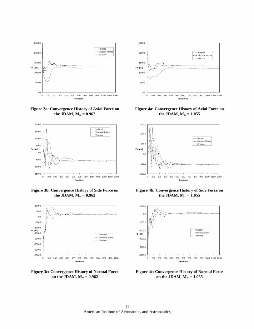
All three grids were used in the transonicsimulations. Figures 3a-c show the convergence

histories for axial force (Fx), side force (Fy) and normalforce (Fz) for the various grids/physics requested. Eachsimulation was run 2,000 iterations, but the solutionsare converged by 800 iterations. These forces arereported in the body-axis system of the entire aircraft.

In addition to grid clustering, Figures 1a-c showpressure contours on the JDAM. A high pressureregion exists at the nose due to the stagnation point.There is another high pressure region at the beginningof the JDAM module; this JDAM module appears tohave a sheet metal base that is attached only to thestore itself. The JDAM module also includes thestrakes. The high pressure region is due to thethickness of this sheet medal plate acting as a forwardfacing ramp, which was obviously modeled in thegrids. The flow then expands as this ramp becomesparallel with the store surface again causing a lowerpressure region. A shock aft of this position causesanother pressure rise. Comparing Figure 1a withFigures 1b and 1c, the shock has clearly movedforward as is expected with the inclusion of viscouseffects.

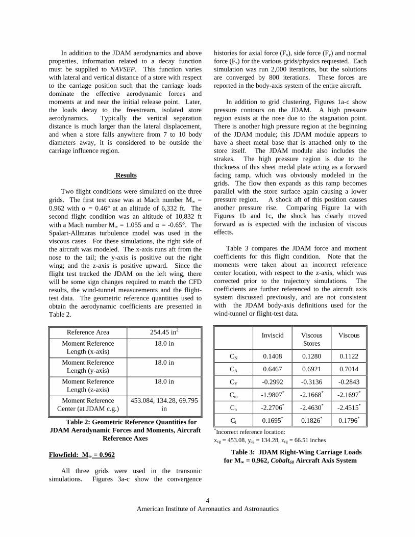
Table 3 compares the JDAM force and momentcoefficients for this flight condition. Note that themoments were taken about an incorrect referencecenter location, with respect to the z-axis, which wascorrected prior to the trajectory simulations. Thecoefficients are further referenced to the aircraft axissystem discussed previously, and are not consistentwith the JDAM body-axis definitions used for thewind-tunnel or flight-test data.

Inviscid ViscousStores

Viscous

CN 0.1408 0.1280 0.1122

CA 0.6467 0.6921 0.7014

CY -0.2992 -0.3136 -0.2843

Cm -1.9807* -2.1668* -2.1697*

Cn -2.2706* -2.4630* -2.4515*

Cl 0.1695* 0.1826* 0.1796*

*Incorrect reference location:xcg = 453.08, ycg = 134.28, zcg = 66.51 inches

Table 3: JDAM Right-Wing Carriage Loadsfor M∞∞ = 0.962, Cobalt60 Aircraft Axis System


Note that the normal force has decreased with theaddition of viscous forces. Axial force has beenincreased in the viscous simulations as expected. Sideforce varied slightly in the three different simulations.There are significant changes in the forces andmoments between the inviscid simulation and theviscous simulations. However, the forces and momentsvary slightly between the viscous stores simulation andthe full viscous simulation. Therefore, to accuratelypredict the carriage loads for an engineering analysis,treating only the stores as viscous seems sufficient.

The inviscid case was simulated on 32 processorsof an IBM SP2. The wall clock time was 4.90 hrs, thesolution time per CPU was 4.87 hrs and the total CPUtime was 155.84 hrs. The viscous stores grid was runon 36 processors of an IBM SP2. This solutionrequired a wall clock time of 4.85 hrs, 4.72 hrs foreach CPU and a total CPU time of 169.78 hrs. Theviscous stores simulation had an average y+ of 4.38.The full viscous case used 50 IBM SP2 processors.This simulation had an average y+ of 3.65. The wallclock time required was 17.69 hrs. The total CPU timewas 861.0 hrs with each CPU requiring 17.22 hrs. Theabove times are for converged solutions at 800iterations.

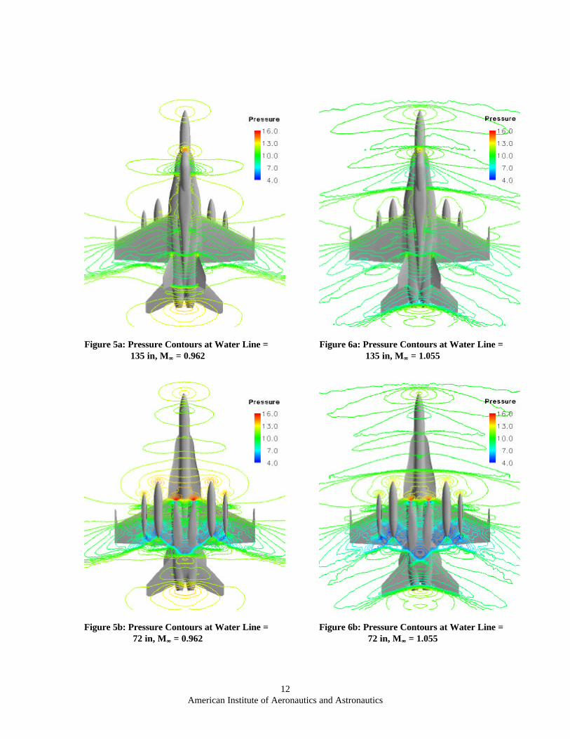
Figure 5a shows pressure contours at a water lineof 135 in, a position above the F/A-18C wing.Notable flow features include the expansion around thefront half of the canopy, a shock wave near the middleof the canopy, and shock waves aft of the boundarylayer diverter. Since the flow has accelerated tosupersonic speeds over the upper fuselage, a shockwave exists in front of the vertical tails due to theirpresence. The interesting shock is the normal shockbetween the trailing edges of the vertical tails. Figure5b shows the complex flowfield interactions below thewing at a water line station of 72 in which intersectsthe JDAM and fuel tank. The expansions due to theJDAM module and the shock wave on the module canclearly be seen. A low pressure region between the aftends of the fuel tank and the JDAM gives rise to theinboard pointing side force. Aft of the two stores,there are a series of intersecting oblique shocks whichthe released JDAM must pass through.

Trajectory: M∞∞ = 0.962

The JDAM carriage loads from the viscousCobalt60 simulation (see Table 3) were transformed tothe correct store body-axis reference system. Thissystem is aligned with the JDAM body axis which is

pitched down 3° with respect to the aircraft axis and iscentered at the JDAM c.g. location. A furthermodification was required to determine forces andmoments for the left-wing configuration. The finalcarriage results, listed in Table 4, are consistent withthe flight-test configuration where the x-axis pointsforward along the JDAM centerline, the y-axis pointsinboard, and the z-axis points downward. Note thatthe normal force is positive in the negative z-direction,and the axial force is positive in the negative x-direction. The pitching moment coefficient fromCobalt60 of Cm = -2.2854 matches the carriage andCTS wind-tunnel measurements of Cm = -2.3, (seeCenko9 for all flight-test data and wind-tunnelmeasurements). The Cobalt60 yawing momentcoefficient result of Cn = -2.4403 falls in the range ofthe carriage Cn = -2.80 and CTS measurement of Cn =-1.55. Cobalt60 calculated a side force coefficient of CY

= 0.2844 which slightly underpredicts the flight-testand wind-tunnel values of CY = 0.31. The normalforce coefficients were measured as CN = 0.15 for theflight test and CN = 0.105 for the wind tunnel whichare slightly larger than the Cobalt60 value of CN =0.0753. Overall, the carriage loads from Cobalt60

matched very well with the flight-test and wind-tunneldata.

CN 0.0753

CA 0.7063

CY 0.2844

Cm -2.2854

Cn -2.4403

Cl 0.0177

Table 4: JDAM Body-Axis Carriage Loads forM∞∞ = 0.962

A series of 5-alpha and 5-beta sweeps for theisolated JDAM were also conducted with Cobalt60, andthe numerical results were placed in a data table forNAVSEP. All the required JDAM properties fromTable 1 and other input parameters such as altitude andMach number were also supplied. Trajectory resultsusing decay functions based on 7-10 diametersexhibited large discrepancies when compared to theflight-test data. Therefore, the decay function wasselected to eliminate the carriage loads effects after theJDAM had fallen about 1-1.5 diameters away from thepylon. This modification suggests that theaerodynamic loads on the JDAM in the transitionregion between carriage and the freestream arechanging rapidly as strong flow gradients exist in the


early stages of release. A grid-based aerodynamic datamatrix or a fully-integrated, moving-mesh CFDcapability may be required to obtain more accuratetrajectories.

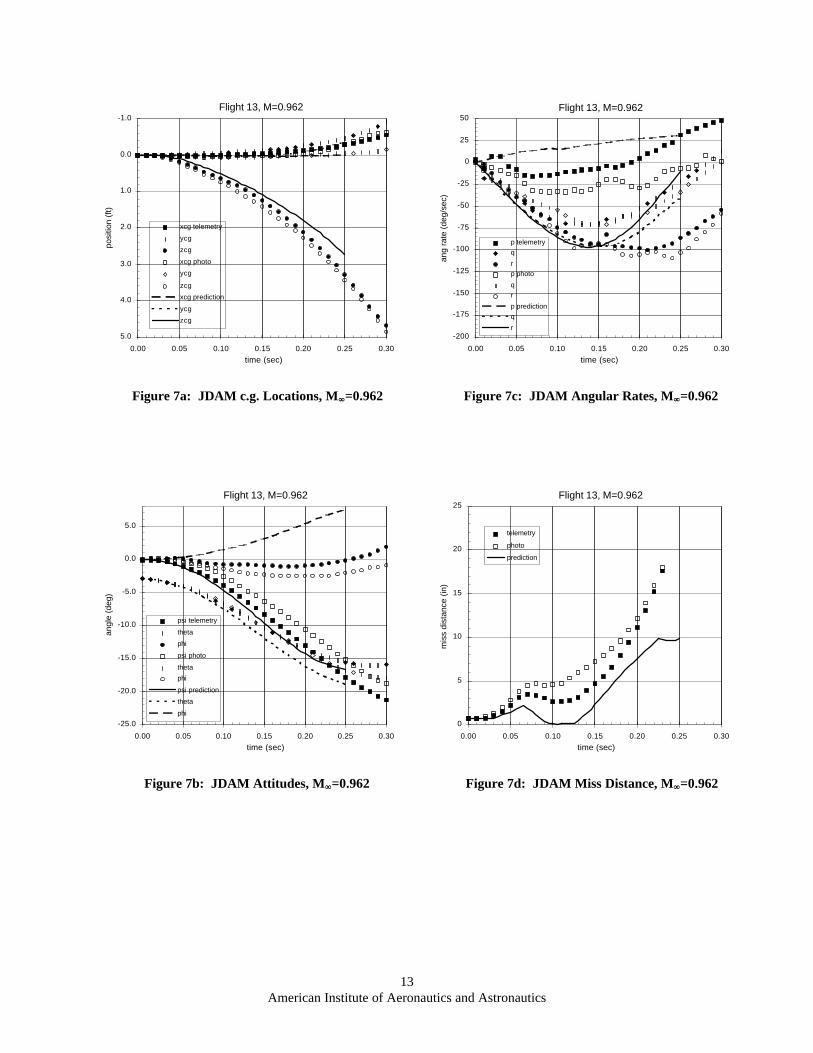
Predicted JDAM trajectory parameters arecompared to the flight-test telemetry andphotogrametric data in Figures 7a-c. Note that theaxial and vertical displacements are underpredicted,whereas the pitch and yaw angles are overpredicted. Aroll reversal occurs during the ejection sequence inflight, as shown by the data in Figure 7c, therefore theroll angle and roll rate are not well predicted by thesimple ejector model used in NAVSEP.

The predicted pitch rate overshoots the maximumflight-test value at about 0.14 sec (see Figure 7c), andthen recovers by 0.25 sec. The predicted yaw raterecovers more rapidly than the flight-test values whichindicate a nearly flat rate between 0.15-0.25 sec.

Figure 7d illustrates the time history of the missdistance, or clearance, between the JDAM and anyportion of the F/A-18C aircraft including the pylonsand fuel tank. Due to the reversed roll attitude seen inthe prediction, the near-zero miss distance between0.1-0.13 sec can be attributed to the JDAM’s upperoutboard fin coming very close to the bottom aft end ofthe pylon.

Flowfield: M∞∞ = 1.055

Simulations on the three grids were completed forthe supersonic case. The convergence histories foraxial force (Fx), side force (Fy) and normal force (Fz)for the various grids/physics requested are shown inFigures 4a-c. Each simulation was run 2,000iterations, but the solutions were again converged by800 iterations. These forces are reported in the body-axis system of the entire aircraft.

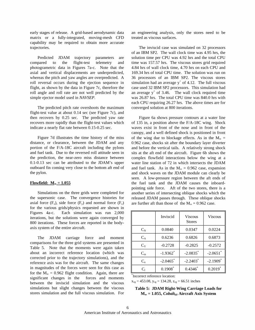
The JDAM carriage force and momentcomparisons for the three grid systems are presented inTable 5. Note that the moments were again takenabout an incorrect reference location (which wascorrected prior to the trajectory simulations), and thereference axis was for the aircraft. The same changesin magnitudes of the forces were seen for this case asfor the M∞ = 0.962 flight condition. Again, there aresignificant changes in the forces and momentsbetween the inviscid simulation and the viscoussimulations but slight changes between the viscousstores simulation and the full viscous simulation. For

an engineering analysis, only the stores need to betreated as viscous surfaces.

The inviscid case was simulated on 32 processorsof an IBM SP2. The wall clock time was 4.95 hrs, thesolution time per CPU was 4.92 hrs and the total CPUtime was 157.57 hrs. The viscous stores grid required4.84 hrs of wall clock time, 4.70 hrs on each CPU and169.34 hrs of total CPU time. The solution was run on36 processors of an IBM SP2. The viscous storessimulation had an average y+ of 4.12. The full viscouscase used 32 IBM SP2 processors. This simulation hadan average y+ of 3.46. The wall clock required timewas 26.87 hrs. The total CPU time was 840.0 hrs witheach CPU requiring 26.27 hrs. The above times are forconverged solution at 800 iterations.

Figure 6a shows pressure contours at a water lineof 135 in, a position above the F/A-18C wing. Shockwaves exist in front of the nose and in front of thecanopy, and a well defined shock is positioned in frontof the wing due to blockage effects. As in the M∞ =0.962 case, shocks sit after the boundary layer diverterand before the vertical tails. A relatively strong shocksits at the aft end of the aircraft. Figure 6b shows thecomplex flowfield interactions below the wing at awater line station of 72 in which intersects the JDAMand fuel tank. As in the M∞ = 0.962 case, expansionand shock waves on the JDAM module can clearly beseen. A low-pressure region between the aft ends ofthe fuel tank and the JDAM causes the inboard-pointing side force. Aft of the two stores, there is aanother series of intersecting oblique shocks which thereleased JDAM passes through. These oblique shocksare further aft than those of the M∞ = 0.962 case.

Inviscid ViscousStores

Viscous

CN 0.0840 0.0347 0.0224

CA 0.6236 0.6826 0.6873

CY -0.2728 -0.2825 -0.2572

Cm -1.9362* -2.0835* -2.0651*

Cn -2.0465* -2.2403* -2.1909*

Cl 0.1908* 0.4346* 0.2019*

*Incorrect reference location:xcg = 453.08, ycg = 134.28, zcg = 66.51 inches

Table 5: JDAM Right-Wing Carriage Loads forM∞∞ = 1.055, Cobalt60 Aircraft Axis System


Trajectory: M∞∞ = 1.055

The JDAM carriage loads from the fully viscouscase (see Table 5) were transformed to the JDAMbody-axis system described previously. A furthermodification was performed to provide loads consistentwith the flight-tested left-wing configuration. Thefinal carriage results are listed in Table 6. The x-axispoints forward along the JDAM centerline, the y-axispoints inboard, and the z-axis points downward. Thepitching moment coefficient for the carriage and CTSwind-tunnel measurements of Cm = -2.15, (see Cenko9

for all flight-test data and wind-tunnel measurements)was slightly overpredicted by the Cobalt60 value of Cm

= -2.2335. The Cobalt60 yawing momentcoefficient result of Cn = -2.2111 falls in the range ofthe carriage Cn = -2.60 and CTS measurement of Cn =-2.15. Cobalt60 predicted a side force coefficient of CY

= 0.2572 which closely approximated the flight-testand wind-tunnel values of CY = 0.25. The normalforce coefficients were measured as CN = 0.05 for theflight test and CN = 0.03 for the wind tunnel which areslightly larger than the Cobalt60 value of CN = -0.0136.Overall, the carriage loads from Cobalt60 matched verywell with the flight-test and wind-tunnel data.

A series of 8-alpha and 5-beta sweeps for theisolated JDAM were also conducted with Cobalt60, andthe numerical results were placed in a data table forNAVSEP. Similar to the previous Mach number case,trajectory predictions using decay functions based on 7-10 diameters exhibited large discrepancies whencompared to the flight-test data. Again, the decayfunction was selected to eliminate the carriage loadseffects after the JDAM had fallen about 1-1.5diameters away from the pylon. Strong flow gradientsexist in the early stages of release, and the transitionregion between carriage and freestream aerodynamicsis difficult to predict. Grid-based studies, integratedmoving-mesh CFD or other influence-based means arerequired to obtain more accurate aerodynamics in thenear-pylon region.

CN -0.0136

CA 0.6876

CY 0.2572

Cm -2.2335

Cn -2.2111

Cl 0.0129

Table 6: JDAM Body-Axis Carriage Loads forM∞∞ = 1.055

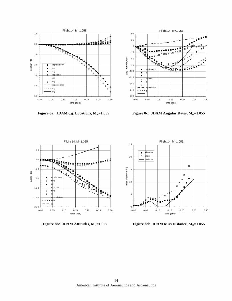
Resulting JDAM trajectory parameters arecompared to the flight-test telemetry andphotogrametric data in Figures 8a-c. Note that the c.g.displacements are well predicted, whereas the pitchand yaw angles are overpredicted as in the previousMach number case. Again, a roll reversal occursduring the ejection sequence in flight (see Figure 8c),therefore the roll angle and roll rate are not wellpredicted by the simple ejector model used in NAVSEP.

The predicted pitch rate overshoots the maximumflight-test value at about 0.15 sec (see Figure 8c), andthen recovers after 0.25 sec. The predicted yaw raterecovers more rapidly than the flight-test values, andby 0.25 sec, this rate is increasing in the oppositedirection. A sudden increase in predicted yaw angle,as shown in Figure 8b, results from the yaw ratereversal.

Figure 8d illustrates the time history of the missdistance between the JDAM and F/A-18C aircraft,including the pylons and fuel tank. Due to thepredicted roll attitude which is opposite to the flight-test data, the near-zero miss distance between 0.1-0.14sec can be attributed to the JDAM’s upper outboard fincoming in very close proximity to the bottom aft end ofthe pylon. Despite the poor prediction of roll angle atabout 0.2 sec, the predicted miss distance is inagreement with the telemetry data.

Conclusions

Store carriage loads for a complex air vehiclesystem were obtained accurately and rapidly usingviscous unstructured-grid CFD methodology. TheCobalt60 flow solver developed by the Air ForceResearch Laboratory was able to resolve relevantcompressible, viscous flow features which dictate theaerodynamic loading. The parallel processing featurein Cobalt60 further enables rapid turnaround time for asingle solution, such that in a week’s time, manycarriage configurations may be simulated during aparametric investigation.

Store separation trajectories were generated withthe Naval Air Warfare Center’s NAVSEP code, aseparate rigid-body, six-degree-of-freedom motionsolver. All CFD-based aerodynamics, as well as storeinertial properties, were simply tabulated and input.The resulting trajectories correlated well with theflight-test data in the earliest stages of release, andthen departed from the data when the carriage effectswere considered to be diminished. Sources of such


discrepancies were likely due to simple ejectormodeling characteristics and general difficulties indetermining suitable aerodynamics in regions ofrapidly changing mutual interference between the storeand parent vehicle.

Acknowledgments

The authors would like to thank J. Garriz and S.Pirzadeh for their help with VGRIDns. All thesimulations in this paper were run using the IBM SP2located at the ASC/MSRC, Wright-Patterson AFB,OH.

References

1. Lijewski, L. and Suhs, N., “Chimera-Eagle StoreSeparation,” AIAA 92-4569, August 1992.

2. Meakin, R. L., “Computations of the UnsteadyFlow About a Generic Wing/Pylon/Finned-StoreConfiguration,” AIAA 92-4568, August 1992.

3. Newman, J. C. and Baysal, O., “TransonicSolutions of a Wing/Pylon/Finned-Store Using HybridDomain Decomposition,” AIAA 92-4571, August1992.

4. Parikh, P., Pirzadeh, S., and Frink, N. T.,“Unstructured Grid Solutions to a Wing/Pylon/StoreConfiguration Using VGRID3D/USM3D,” AIAA 92-4572, August 1992.

5. Jordan, J. K., “Computational Investigation ofPredicted Store Loads in Mutual Interference FlowFields,” AIAA 92-4570, August 1992.

6. Madson, M. and Talbot, M., “F-16/GenericCarriage Load Predictions at Transonic Mach Numbersusing TRANAIR,” AIAA 96-2454, June 1996.

7. Cline, D., Riner, W., Jolly, B., and Lawrence, W.,“Calculation of Generic Store Separations from an F-16 Aircraft,” AIAA 96-2455, June 1996.

8. Kern, S. B. and Bruner, C. W. S., “ExternalCarriage Analysis of a Generic Finned-Store on the F-16 Using USM3D,” AIAA 96-2456, June 1996.

9. Cenko, A., “F-18/JDAM CFD Challenge WindTunnel Flight Test Results,” AIAA 99-0120, January1999.

10. Strang, W. Z., Tomaro, R. F., and Grismer, M. J.,“The Defining Methods of Cobalt60: A Parallel,Implicit, Unstructured Euler/Navier-Stokes FlowSolver,” AIAA 99-0786, January 1999.

11. Godunov, S. K., “A Difference Scheme forNumerical Computation of Discontinuous Solution ofHydrodynamic Equations,” Sbornik Mathematics, vol47, p. 271-306, 1959.

12. Spalart, P. R. and Allmaras, S. R., “A One-Equation Turbulence Model for Aerodynamic Flows,”AIAA 92-0439, January 1992.

13. Baldwin, B. S. and Barth, T. J., “A One-EquationTurbulence Transport Model for High ReynoldsNumber Wall-Bounded Flows,” NASA TM 102847,August 1990.

14. Tomaro, R. F, Strang, W. Z., and Sankar. L. N.,“An Implicit Algorithm for Solving Time DependentFlows on Unstructured Grids,” AIAA 97-0333, January1997.

15. Grismer, M. J., Strang, W. Z., Tomaro, R. F., andWitzeman, F. C., “Cobalt: A Parallel, Implicit,Unstructured Euler/Navier-Stokes Solver,” Advancesin Engineering Software, Vol 29, No. 3-6, pp. 365-373,Apr-Jul 1998.

16. Strang, W.Z., “Parallel Cobalt60 User’s Manual,”AFRL/VAAC, WPAFB, OH, August 1998.

17. Pirzadeh, S., “Three-Dimensional UnstructuredViscous Grids by the Advancing-Layers Method,”AIAA Journal, Vol. 34, No. 1, January 1996, p. 43-49.

18. Cenko, A., private communication, January 1998.

19. Carmen Jr., J. B., Hill Jr., D. W., and Christopher,J. P., “Store Separation Testing Techniques at theArnold Engineering Development Center, Vol II,Description of Captive Trajectory Store SeparationTesting in the Aerodynamic Wind-Tunnel (4T),”AEDC-TR-79-1, June 1980.


Figure 1a: Inviscid Grid Near the JDAM and the Outboard Pylon

Figure 1b: Viscous Stores Grid Near the JDAM and the Outboard Pylon

Figure 1c: Viscous Grid Near the JDAM and the Outboard Pylon


Figure 2a: Viscous Grid Clustering at a Fuselage Station through the JDAM

Figure 2b: Viscous Grid Clustering at a Water Line through the JDAM


0.0

500.0

1000.0

1500.0

2000.0

2500.0

0 100 200 300 400 500 600 700 800 900 1000 1100 1200

Iterations

Fx (psi)

InviscidViscous StoresViscous

Figure 3a: Convergence History of Axial Force onthe JDAM, M∞∞ = 0.962

-1500.0

-1000.0

-500.0

0.0

500.0

1000.0

1500.0

2000.0

0 100 200 300 400 500 600 700 800 900 1000 1100 1200

Iterations

Fy (psi)


Figure 3b: Convergence History of Side Force onthe JDAM, M∞∞ = 0.962

-3500.0

-3000.0

-2500.0

-2000.0

-1500.0

-1000.0

-500.0

0.0

500.0

1000.0

0 100 200 300 400 500 600 700 800 900 1000 1100 1200

Iterations

Fz (psi)


Figure 3c: Convergence History of Normal Forceon the JDAM, M∞∞ = 0.962

0.0

500.0

1000.0

1500.0

2000.0

2500.0

0 100 200 300 400 500 600 700 800 900 1000 1100 1200

Iterations

Fx (psi)


Figure 4a: Convergence History of Axial Force onthe JDAM, M∞∞ = 1.055

-1000.0

-500.0

0.0

500.0

1000.0

1500.0

0 100 200 300 400 500 600 700 800 900 1000 1100 1200

Iterations

Fy (psi)


Figure 4b: Convergence History of Side Force onthe JDAM, M∞∞ = 1.055

-5000.0

-4000.0

-3000.0

-2000.0

-1000.0

0.0

1000.0

0 100 200 300 400 500 600 700 800 900 1000 1100 1200

Iterations

Fz (psi)


Figure 4c: Convergence History of Normal Forceon the JDAM, M∞∞ = 1.055


Figure 5a: Pressure Contours at Water Line =135 in, M∞∞ = 0.962

Figure 5b: Pressure Contours at Water Line =72 in, M∞∞ = 0.962

Figure 6a: Pressure Contours at Water Line =135 in, M∞∞ = 1.055

Figure 6b: Pressure Contours at Water Line =72 in, M∞∞ = 1.055


Flight 13, M=0.962-1.0

0.0

1.0

2.0

3.0

4.0

5.0

0.00 0.05 0.10 0.15 0.20 0.25 0.30

time (sec)

posi

tion

(ft)

xcg telemetry

ycg

zcg

xcg photo

ycg

zcg

xcg prediction

ycg

zcg

Figure 7a: JDAM c.g. Locations, M∞∞=0.962

Flight 13, M=0.962

-25.0

-20.0

-15.0

-10.0

-5.0

0.0

5.0

0.00 0.05 0.10 0.15 0.20 0.25 0.30

time (sec)

angl

e (d

eg)

psi telemetry

theta

phi

psi photo

theta

phi

psi prediction

theta

phi

Figure 7b: JDAM Attitudes, M∞∞=0.962

Flight 13, M=0.962

-200

-175

-150

-125

-100

-75

-50

-25

0

25

50

0.00 0.05 0.10 0.15 0.20 0.25 0.30

time (sec)

ang

rate

(de

g/se

c)

p telemetry

q

r

p photo

q

r

p prediction

q

r

Figure 7c: JDAM Angular Rates, M∞∞=0.962

Flight 13, M=0.962

0

5

10

15

20

25

0.00 0.05 0.10 0.15 0.20 0.25 0.30

time (sec)

mis

s di

stan

ce (

in)

telemetry

photo

prediction

Figure 7d: JDAM Miss Distance, M∞∞=0.962


Flight 14, M=1.055-1.0

0.0

1.0

2.0

3.0

4.0

5.0

0.00 0.05 0.10 0.15 0.20 0.25 0.30

time (sec)

posi

tion

(ft)

xcg telemetry

ycg

zcg

xcg photo

ycg

zcg

xcg prediction

ycg

zcg

Figure 8a: JDAM c.g. Locations, M∞∞=1.055

Flight 14, M=1.055

-25.0

-20.0

-15.0

-10.0

-5.0

0.0

5.0

0.00 0.05 0.10 0.15 0.20 0.25 0.30

time (sec)

angl

e (d

eg)

psi telemetry

theta

phi

psi photo

theta

phi

psi prediction

theta

phi

Figure 8b: JDAM Attitudes, M∞∞=1.055

Flight 14, M=1.055

-200

-175

-150

-125

-100

-75

-50

-25

0

25

50

0.00 0.05 0.10 0.15 0.20 0.25 0.30

time (sec)

ang

rate

(de

g/se

c)

p telemetry

q

r

p photo

q

r

p prediction

q

r

Figure 8c: JDAM Angular Rates, M∞∞=1.055

Flight 14, M=1.055

0

5

10

15

20

25

0.00 0.05 0.10 0.15 0.20 0.25 0.30

time (sec)

mis

s di

stan

ce (

in)

telemetry

photo

prediction

Figure 8d: JDAM Miss Distance, M∞∞=1.055

Documents

AIAA 99-0122 A Solution on the F-18C for Store Separation