AI-Driven CT-based quantification, staging andshort-term outcome prediction of COVID-19pneumoniaGuillaume Chassagnon, MD PhD*,1,2,3, Maria Vakalopoulou, PhD∗4,5,6,7, Enzo Battistella,MsC4,6,7, Stergios Christodoulidis, PhD8,9, Trieu-Nghi Hoang-Thi, MD1, SeverineDangeard, MD1, Eric Deutsch, MD PhD6,7, Fabrice Andre, MD PhD8,9, Enora Guillo, MD1,Nara Halm, MD1, Stefany El Hajj, MD1, Florian Bompard, MD1, Sophie Neveu, MD1,Chahinez Hani, MD1, Ines Saab, MD1, Alienor Campredon, MD1, Hasmik Koulakian, MD1,Souhail Bennani, MD1, Gael Freche, MD1, Aurelien Lombard, MsC15, Laure Fournier, MDPhD2,10, Hippolyte Monnier, MD10, Teodor Grand, MD10, Jules Gregory, MD2,11, AntoineKhalil, MD PhD2,12, Elyas Mahdjoub, MD2,12, Pierre-Yves Brillet, MD PhD13, StephaneTran Ba, MD13, Valerie Bousson, MD PhD2,14, Marie-Pierre Revel, MD PhD1,2,3, and NikosParagios, PhD†4,7,15

1Radiology Department, Hopital Cochin – AP-HP.Centre Universite de Paris, 27 Rue du Faubourg Saint-Jacques,75014 Paris, France2Universite de Paris, 85 boulevard Saint-Germain, 75006 Paris, France3Inserm U1016, Institut Cochin, 22 rue Mechain, 75014 Paris, France4Universite Paris-Saclay, CentraleSupelec, Mathematiques et Informatique pour la Complexite et les Systemes,Gif-sur-Yvette, France, 3 Rue Joliot Curie, 91190 Gif-sur-Yvette, France5Universite Paris-Saclay, CentraleSupelec, Inria, Gif-sur-Yvette, France6Universite Paris-Saclay, Institut Gustave Roussy, Inserm 981 Molecular Radiotherapy and Innovative Therapeutics,114 Rue Edouard Vaillant, 94800 Villejuif, France7Gustave Roussy-CentraleSupelec-TheraPanacea, Noesia Center of Artificial Intelligence in Radiation Therapy andOncology, Gustave Roussy Cancer Campus, Villejuif, France8Universite Paris-Saclay, Institut Gustave Roussy, Inserm 1030 Predictive Biomarkers and New TherapeuticStrategies in Oncology, 114 Rue Edouard Vaillant, 94800 Villejuif, France9Universite Paris-Saclay, Institut Gustave Roussy, Prism Precision Medicine Center, 114 Rue Edouard Vaillant,94800 Villejuif, France10Radiology Department, Hopital Europeen Georges Pompidou – AP-HP.Centre Universite de Paris, 20 RueUniversite Paris-Saclay, 75015 Paris, France11Radiology Department, Hopital Beaujon – AP-HP.Nord Universite de Paris, 100 Boulevard du General Leclerc,92110 Clichy12Radiology Department, Hopital Bichat – AP-HP.Nord Universite de Paris, 46 Rue Henri Huchard, 75018 Paris,France13Radiology Department, Hopital Avicenne – AP-HP.Hopitaux universitaires Paris Seine-Saint-Denis, 125 Rue deStalingrad, 93000 Bobigny, France14Radiology Department, Hopital Lariboisiere – AP-HP.Nord Universite de Paris, 2 Rue Ambroise Pare, 75010 Paris,France15TheraPanacea, 27 Rue du Faubourg Saint-Jacques, 75014 Paris, France

∗Dr. Guillaume Chassagnon & Dr. Maria Vakalopoulou have equally contributed to this work†Corresponding author: n.paragios@therapanacea.eu

arX

iv:2

004.

1285

2v1

[cs

.CV

] 2

0 A

pr 2

020

ABSTRACT

Chest computed tomography (CT) is widely used for the management of Coronavirus disease 2019 (COVID-19) pneumoniabecause of its availability and rapidity1–3 . The standard of reference for confirming COVID-19 relies on microbiological testsbut these tests might not be available in an emergency setting and their results are not immediately available, contrary to CT. Inaddition to its role for early diagnosis, CT has a prognostic role by allowing visually evaluating the extent of COVID-19 lungabnormalities4,5. The objective of this study is to address prediction of short-term outcomes, especially need for mechanicalventilation. In this multi-centric study, we propose an end-to-end artificial intelligence solution for automatic quantification andprognosis assessment by combining automatic CT delineation of lung disease meeting expert’s performance and data-drivenidentification of biomarkers for its prognosis. AI-driven combination of variables with CT-based biomarkers offers perspectivesfor optimal patient management given the shortage of intensive care beds and ventilators6,7.

Main

COVID-19 has emerged in December 2019 in the city of Wuhan in China8 and disseminated around the world, leading theWorld Health Organization to declare the COVID-19 outbreak a pandemic. The disease is caused by the SARS-Cov-2 virusand the leading cause of death is respiratory failure due to severe viral pneumonia9. Chest computed tomography (CT) hasrapidly gained a major role for COVID-19 diagnosis. Indeed, despite being considered as the gold standard to make a definitivediagnosis, reverse transcription polymerase chain reaction (RT-PCR) suffers from false negatives, shortage of available supplytest kits and long turnaround times10–12.

Artificial intelligence has gained significant attention during the past decade and many applications have been proposed inmedical imaging, including segmentation and characterization tasks such as lung cancer screening on CT13–15. A few studieshave already reported deep learning to diagnose COVID-19 pneumonia on chest radiograph16 or CT17 . Other authors used

Figure 1. Overview of the method for CT-based quantification, staging and prognosis of COVID-19. (i) Two independentcohorts with quantification based on ensemble 2D & 3D consensus neural networks reaching expert-level annotations onmassive evaluation, (ii) Consensus-driven bio(imaging)-marker selection on the principle of prevalence across methods leadingto variables highly-correlated with outcomes & (iii) Consensus of linear & non-linear classification methods for staging andprognosis reaching optimal performance (minimum discrepancy between training & testing).

Figure 2. Comparison between automated and manual segmentations. Delineation of the diseased areas on chest CT in aCOVID-19 patient: First Row: input, AI-segmentation, expert I-segmentation, expert II-segmentation. Second Row: Box-PlotComparisons in terms of Dice similarity and Haussdorf between AI-solution, expert I & expert II, & Plot of correlationbetween disease extent automatically measured and the average disease extent measured from the 2 manual segmentations.Disease extent is expressed as the percentage of lung affected by the disease. Third row: statistical measures on comparisonsbetween AI, expert I, and expert II segmentations.

deep-learning to quantify COVID-19 disease extent on CT but none of them used a multi-centric cohort while providingcomparisons with segmentations done by radiologists18, 19. Disease extent is the only parameter that can be visually estimatedon chest CT to quantify disease severity4, 5, but visual quantification is difficult and usually coarse. Several AI-based tools havebeen recently developed to quantify interstitial lung diseases (ILD)20–23, which share common CT features with COVID-19pneumonia, especially a predominance of ground glass opacities. In this study, we investigated a fully automatic method(Figure 1) for disease quantification, staging and short-term prognosis. The approach relied on (i) a disease quantificationsolution that exploited 2D & 3D convolutional neural networks using an ensemble method, (ii) a biomarker discovery approachsought to determine the share space of features that are the most informative for staging & prognosis, & (iii) an ensemblerobust supervised classification method to distinguish patients with severe vs non-severe short-term outcome and among severepatients those intubated and those who did not survive.

Part I: Disease QuantificationIn the context of this work, we report a deep learning-based segmentation tool to quantify COVID-19 disease and lung volume.For this purpose, we used an ensemble network approach inspired by the AtlasNet framework22. We investigated a combinationof 2D slice-based24 and 3D patch-based ensemble architectures25. The development of the deep learning-based segmentationsolution was done on the basis of a multi-centric cohort of 478 unenhanced chest CT scans (208,668 slices) of COVID-19

3/16

Figure 3. Spider-chart distribution of features depicting their minimum and maximum values [mean value (blue), 70%percentile (yellow) and 90% percentile (red) lines] with respect to the different outcomes with the following order: top:non-severe, bottom left: intensive care support & bottom right: deceased in the testing set. White and red circles representrespectively 40% and 60% of the maximum value of each feature. Clear separation was observed on these feature space withrespect to the non-severe & severe cases. In terms of deceased versus intensive care patients, notable difference were observedwith respect to three variables, the age of the patient, the condition of the healthy lung and the non-uniformity of the disease(indicated with gray in the spider-chart).

patients with positive RT-PCR. The multicentric dataset was acquired at 6 Hospitals, equipped with 4 different CT modelsfrom 3 different 91 manufacturers, with different acquisition protocols and radiation dose (Table 1). Fifty CT exams from 3centers were used for training and 130 CT exams from 3 other centers were used for test (Table 2). Disease and lung weredelineated on all 23,423 images used as training dataset, and on only 20 images per exam but by 2 independent annotators inthe test dataset (2,600 images). The overall annotation effort took approximately 800 hours and involved 15 radiologists with 1to 7 years of experience in chest imaging. The consensus between manual (2 annotators) and automated segmentation wasmeasured using the Dice similarity score (DSC)26 and the Haussdorf distance (HD). The CovidENet performed equally well totrained radiologists in terms of DSCs and better in terms HD (Figure 2). The mean/median DSCs between the two expert’sannotations on the test dataset were 0.70/0.72 for disease segmentation. For the same task, DSCs between CovidENet and themanual segmentations were 0.69/0.71 and 0.70/0.73. In terms of HDs, the observed average value between the two expertswas 9.16mm while it was 8.96mm between CovidENet and the two experts. When looking at disease extent, defined as thepercentage of lung affected by the disease, we found no significant difference between automated segmentation and the averageof the two manual segmentations (19.9% ±17.7 [0.5−73.2] vs 19.5% ±16.5 [1.1−75.7]; p= 0.352).

Part II: Imaging Biomarker DiscoveryTo assess the prognostic value of the Chest computed tomography (CT) an extended multi-centric data set was built. Wereviewed outcomes in patient charts within the 4 days following chest CT and divided the patients in 3 groups: those whodidn’t survive, those who required mechanical ventilation and those who were still alive and not intubated. Out of the 478included patients, 27 died (6%) and 83 were intubated (17%), forming a group of 110 patients with severe short-term outcome(23%). Data of 383 patients from 3 centers were used for training and those of 85 patients from 3 other centers composed

4/16

Figure 4. Classification performance of dual & aggregated classifiers with respect to the non-severe vs severe case, theintubated vs deceased case and the three classes. Sensitivity and confusion tables are presented with respect to the differentclassification problems.

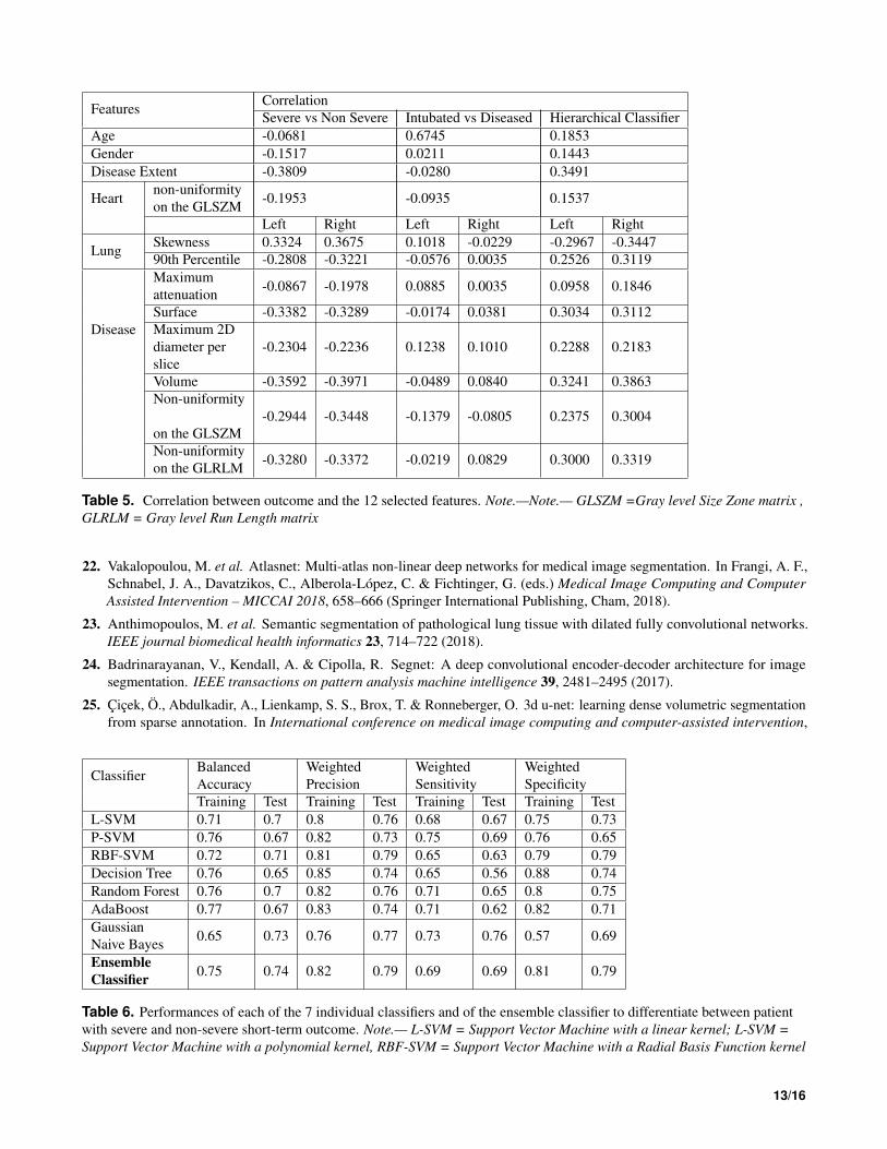
an independent test dataset (Table 3). Radiomics-based prognosis gained significant attention in the recent years towardspredicting treatment outcomes27. In this study we have adopted a similar strategy, we extracted 107 features related to firstorder, higher order statistics, texture and shape information for lungs, disease extent and heart. Feature selection was performedon a basis of predictive value consensus. We created several representative partitions 117 of the training set (80% training and20% validation) and run 13 different supervised classification methods towards optimal separation of the observed clinicalground truth between severe and non-severe cases (Table 4). The features that were shared between the different classifierswere retained as robust imaging biomarkers using a cut-off probability of 0.25 and were aggregated to patients’ age and gender(Table 5). In total 12 features were retained for the prognosis part and included age, gender, disease extent, descriptors ofdisease heterogeneity and extension, features of healthy lung and a descriptor of cardiac heterogeneity. Correlations for somethese features and the clinical outcome are presented in Figure 5 while a representation of these feature space with respect tothe different classes is presented in Figure 3.

Part III: Staging and PrognosisThe staging/prognosis was implemented using a hierarchical classification principle, targeting first staging and subsequentlyprognosis. The staging component sought to separate patients with severe and non-severe short-term outcomes, while theprognosis sought to predict the risk of decease among severe patients. On the basis of the feature selection step, the machinelearning algorithms that had a balanced accuracy greater than 60% on validation were considered. The selection of thesemethods was done on the basis of minimum discrepancy between performance on training and internal validation sub-trainingdata set. We have built two sequential classifiers using this ensemble method, one to determine the severe cases and a second topredict survival. The classifier aiming to separate patients with severe and non-severe short-term outcomes had a balancedaccuracy of 74%, a weighted precision of 79%, a weighted sensitivity of 69% and specificity of 79% to predict a severeshort-term outcome (Figure 4, Table 6). The performance of the second classifier aiming to differentiate between intubated anddeceased patients was even higher with a balanced accuracy of 81% (Figure 4, Table 7). The hierarchical classifiers combingthe 3 classes had a balanced accuracy of 68%, a weighted precision of 79%, a weighted sensitivity of 67% and specificityof 83% (Figure 4). It was observed that prognosis performance difference between training and external cohort testing waslow, suggesting that the most important information present at CT scans was recovered, and additional information should beintegrated in order to fully explain the outcome.

Part IV: ConclusionsIn conclusion, artificial intelligence enhanced the value of chest CT by providing fast accurate, and precise disease extentquantification and by helping to identify patients with severe short-term outcomes. This could be of great help in the currentcontext of the pandemic with healthcare resources under extreme pressure. In a context where the sensitivity of RT-PCR has

5/16

Figure 5. Discovery of – imaging-biomarkers through consensus. Generic variables (G: age, sex), disease related variables (D:extent, volume, maximum diameter, etc.), lung variables (L: skewness, etc.) as well as heart related variables (H:non-uniformity) have been automatically selected. The prevalence of the features as well as their distribution with respect to thedifferent classes is presented for some of them, with rather clear separation and strong correlations with ground truth.

been shown to be low, such as 63% when perform on nasal swab28, chest CT has been shown to provide higher sensitivity fordiagnosis of COVID-19 as compared with initial RT-PCR from pharyngeal swab samples10. The current COVID-19 pandemicrequires implementation of rapid clinical triage in healthcare facilities to categorize patients into different urgency categories29,often occurring in the context of limited access to biological tests. Beyond the diagnostic value of CT for COVID-19, our studysuggests that AI should be part of the triage process. The developed tool will be made publicly available. Our prognosis andstaging method achieved state of the art results through the deployment of a highly robust ensemble classification strategywith automatic feature selection of imaging biomarkers and patients’ characteristics available within the image’ metadata. Interms of future work, the continuous enrichment of the data base with new examples is a necessary action on top of updatingthe outcome of patients included in the study. The integration of non-imaging data and other related clinical and categoricalvariables such as lymphopenia, the D-dimer level and other comorbidities9, 30–32 is a necessity towards better understanding thedisease and predicting the outcomes. This is clearly demonstrated from the inability of any of the state-of-the art classificationmethods (including neural networks and multi-layer perceptron models) to predict the outcome with a balanced accuracy greaterto 80% on the training data. Our findings could have a strong impact in terms of (i) patient stratification with respect to thedifferent therapeutic strategies, (ii) accelerated drug development through rapid, reproducible and quantified assessment oftreatment response through the different mid/end-points of the trial, and (iii) continuous monitoring of patient’s response totreatment.

6/16

MethodsStudy Design and ParticipantsThis retrospective multi-center study was approved by our Institutional Review Board (AAA-2020-08007) which waived theneed for patients’ consent. Patients diagnosed with COVID-19 from March 4th to 29th at six large University Hospitals wereeligible if they had positive PCR-RT and signs of COVID-19 pneumonia on unenhanced chest CT. A total of 478 patientsformed the full dataset (208,668 CT slices). Only one CT examination was included for each patient. Exclusion criteria were(i) contrast medium injection and (ii) important motion artifacts.

For the COVID-19 radiological pattern segmentation part, 50 patients from 3 centers (A: 20 patients; B: 15 patients, C:15 patients) were included to compose a training and validation dataset, 130 patients from the remaining 3 centers (D: 50patients; E: 50 patients, F: 30 patients) were included to compose the test dataset (Table 2). The proportion between the CTmanufacturers in the datasets was pre-determined in order to maximize the model generalizability while taking into account thedata distribution.

For the radiomics driven prognosis study, 298 additional patients from centers A (96 patients), B (64 patients) and D (138patients) were included to increase the size of the dataset. Data of 383 patients from 3 centers (A, B and D) were used fortraining and those of 85 patients from 3 other centers (C, E, F) composed an independent test set (Table 3). Only one CTexamination was included for each patient. Exclusion criteria were (i) contrast medium injection and (ii) important motionartifacts. For short-term outcome assessment, patients were divided into 2 groups: those who died or were intubated in the 4days following the CT scan composed the severe short-term outcome subgroup, while the others composed the non-severeshort-term outcome subgroup.

CT AcquisitionsChest CT exams were acquired on 4 different CT models from 3 manufacturers (Aquilion Prime from Canon Medical Systems,Otawara, Japan; Revolution HD from GE Healthcare, Milwaukee, WI; Somatom Edge and Somatom AS+ from SiemensHealthineer, Erlangen, Germany). The different acquisition and reconstruction parameters are summarized in Table 1. CTexams were mostly acquired at 120 (n=103/180; 57%) and 100 kVp (n=76/180; 42%). Images were reconstructed usingiterative reconstruction with a 512×512 matrix and a slice thickness of 0.625 or 1 mm depending on the CT equipment. Onlythe lung images reconstructed with high frequency kernels were used for analysis. For each CT examination, dose lengthproduct (DLP) and volume Computed Tomography Dose Index (CTDIvol) were collected.

Data AnnotationFifteen radiologists (GC, TNHT, SD, EG, NH, SEH, FB, SN, CH, IS, HK, SB, AC, GF and MB) with 1 to 7 years of experiencein chest imaging participated in the data annotation which was conducted over a 2-week period. For the training and validationset for the COVID-19 radiological pattern segmentation, the whole CT examinations were manually annotated slice by sliceusing the open source software ITKsnap 1. On each of the 23,423 axial slices composing this dataset, all the COVID-19related CT abnormalities (ground glass opacities, band consolidations, and reticulations) were segmented as a single class.Additionally, the whole lung was segmented to create another class (lung). To facilitate the collection of the ground truth for thelung anatomy, a preliminary lung segmentation was performed with Myrian XP-Lung software (version 1.19.1, Intrasense,Montpellier, France) and then manually corrected.

As far as test cohort for the segmentation is concerned, 20 CT slices equally spaced from the superior border of aortic archto the lowest diaphragmatic dome were selected to compose a 2,600 images dataset. Each of these images were systematicallyannotated by 2 out of the 15 participating radiologists who independently performed the annotation. Annotation consisted ofmanual delineation of the disease and manual segmentation of the lung without using any preliminary lung segmentation.

Deep Learning ConstructionThe segmentation tool was built under the paradigm of ensemble methods using a 2D fully convolutional network together withthe AtlasNet framework22 and a 3D fully convolutional network25. The AtlasNet framework combines a registration stage ofthe CT scans to a number of anatomical templates and consequently utilizes multiple deep learning-based classifiers trained foreach template. At the end, the prediction of each model is - to the original anatomy and a majority voting scheme is used toproduce the final projection, combining the results of the different networks. A major advantage of the AtlasNet framework isthat it incorporates a natural data augmentation by registering each CT scan to several templates. Moreover, the frameworkis agnostic to the segmentation model that will be utilized. For the registration of the CT scans to the templates, an elasticregistration framework based on Markov Random Fields was used, providing the optimal displacements for each template33.

The architecture of the implemented segmentation models was based on already established fully convolutional neuralnetwork designs from the literature24, 25. Fully convolutional networks following an encoder decoder architecture both in 2D

1http://www.itksnap.org

7/16

and 3D were developed and evaluated. For the 2D models the CT scans were separated on the axial view. The network included5 convolutional blocks, each one containing two Conv-BN-ReLU layer successions. Maxpooling layers were also distributedat the end of each convolutional block for the encoding part. Transposed convolutions were used on the decoding part torestore the spatial resolution of the slices together with the same successions of layers. For the 3D pipeline, the model similarlyconsisted of five blocks with a down-sampling operation applied every two consequent Conv3D-BN-ReLU layers. Additionally,five decoding blocks were utilized for the decoding path, at each block a transpose convolution was performed in order toup-sample the input. Skip connections were also employed between the encoding and decoding paths. In order to train thismodel, cubic patches of size 64×64×64 were randomly extracted within a close range of the ground truth annotation borderin a random fashion. Corresponding cubic patches were also extracted from the ground truth annotation masks and the lunganatomy segmentation masks. To this end, we trained the model with the CT scan patch as input, the annotation patch as targetand the lung anatomy annotation patch as a mask for calculating the loss function only within the lung region. In order to trainall the models, each CT scan was normalized by cropping the Hounsfield units in the range [−1024, 1000].

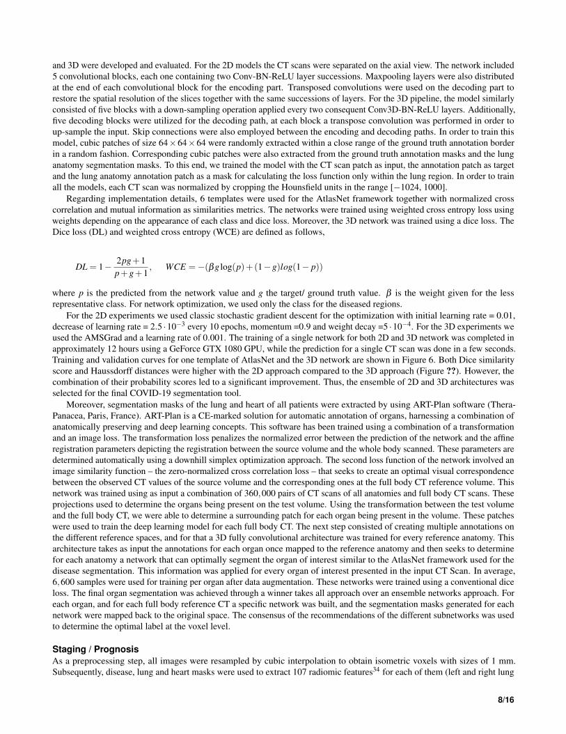
Regarding implementation details, 6 templates were used for the AtlasNet framework together with normalized crosscorrelation and mutual information as similarities metrics. The networks were trained using weighted cross entropy loss usingweights depending on the appearance of each class and dice loss. Moreover, the 3D network was trained using a dice loss. TheDice loss (DL) and weighted cross entropy (WCE) are defined as follows,

DL = 1− 2pg+1p+g+1

, WCE =−(βg log(p)+(1−g)log(1− p))

where p is the predicted from the network value and g the target/ ground truth value. β is the weight given for the lessrepresentative class. For network optimization, we used only the class for the diseased regions.

For the 2D experiments we used classic stochastic gradient descent for the optimization with initial learning rate = 0.01,decrease of learning rate = 2.5 ·10−3 every 10 epochs, momentum =0.9 and weight decay =5 ·10−4. For the 3D experiments weused the AMSGrad and a learning rate of 0.001. The training of a single network for both 2D and 3D network was completed inapproximately 12 hours using a GeForce GTX 1080 GPU, while the prediction for a single CT scan was done in a few seconds.Training and validation curves for one template of AtlasNet and the 3D network are shown in Figure 6. Both Dice similarityscore and Haussdorff distances were higher with the 2D approach compared to the 3D approach (Figure ??). However, thecombination of their probability scores led to a significant improvement. Thus, the ensemble of 2D and 3D architectures wasselected for the final COVID-19 segmentation tool.

Moreover, segmentation masks of the lung and heart of all patients were extracted by using ART-Plan software (Thera-Panacea, Paris, France). ART-Plan is a CE-marked solution for automatic annotation of organs, harnessing a combination ofanatomically preserving and deep learning concepts. This software has been trained using a combination of a transformationand an image loss. The transformation loss penalizes the normalized error between the prediction of the network and the affineregistration parameters depicting the registration between the source volume and the whole body scanned. These parameters aredetermined automatically using a downhill simplex optimization approach. The second loss function of the network involved animage similarity function – the zero-normalized cross correlation loss – that seeks to create an optimal visual correspondencebetween the observed CT values of the source volume and the corresponding ones at the full body CT reference volume. Thisnetwork was trained using as input a combination of 360,000 pairs of CT scans of all anatomies and full body CT scans. Theseprojections used to determine the organs being present on the test volume. Using the transformation between the test volumeand the full body CT, we were able to determine a surrounding patch for each organ being present in the volume. These patcheswere used to train the deep learning model for each full body CT. The next step consisted of creating multiple annotations onthe different reference spaces, and for that a 3D fully convolutional architecture was trained for every reference anatomy. Thisarchitecture takes as input the annotations for each organ once mapped to the reference anatomy and then seeks to determinefor each anatomy a network that can optimally segment the organ of interest similar to the AtlasNet framework used for thedisease segmentation. This information was applied for every organ of interest presented in the input CT Scan. In average,6,600 samples were used for training per organ after data augmentation. These networks were trained using a conventional diceloss. The final organ segmentation was achieved through a winner takes all approach over an ensemble networks approach. Foreach organ, and for each full body reference CT a specific network was built, and the segmentation masks generated for eachnetwork were mapped back to the original space. The consensus of the recommendations of the different subnetworks was usedto determine the optimal label at the voxel level.

Staging / PrognosisAs a preprocessing step, all images were resampled by cubic interpolation to obtain isometric voxels with sizes of 1 mm.Subsequently, disease, lung and heart masks were used to extract 107 radiomic features34 for each of them (left and right lung

8/16

were considered separately both for the disease extent and entire lung). The features included first order statistics, shape-basedfeatures in 2D and 3D together with texture-based features. Radiomics features were enriched with clinical data available fromthe image metadata (age, gender), disease extent and number of diseased regions. The minimum and maximum values werecalculated for the training and validation cohorts and Min-Max normalization was used to normalize the features, the samevalues were also applied on the test set. As a first step, a number of features were selected using a lasso linear model in order todecrease the dimensionality. The lasso estimator seeks to optimize the following objective function:

||y−Xw||222n

+α||w||1

where α is a constant, ||w||1 is the L1-norm of the coefficient vector and n is the number of samples. The Lasso methodwas used with 200 alphas along a regularization path of length 0.01 and limited to 1000 iterations. The staging/prognosiscomponent was addressed using an ensemble learning approach. First, the training data set was subdivided into training andvalidation set on the principle of 80%− 20% while respecting that the distribution of classes between the two subsets wasidentical to the observed one. We have created 10 subdivisions on this basis and evaluated the average performance of thefollowing supervised classification methods: Nearest Neighbor, {Linear, Sigmoid, Radial Basis Function, Polynomial Kernel}Support Vector Machines, Gaussian Process, Decision Trees, Random Forests, AdaBoost, Gaussian Naive Bayes, BernoulliNaive Bayes, Multi-Layer Perceptron & Quadratic Discriminant Analysis. Features selection was performed on the training setof each subdivision. In particular, the features selected in at least three subdivision were considered critical and have been usedlater for the staging and prognosis.

• Age

• Gender

• Disease Extent

• From the diseased areas: maximum attenuation, surface, maximum 2D diameter per slice, volume, non-uniformity of theGray level Size Zone matrix (GLSZM) and non-uniformity of the Gray level Run Length matrix (GLRLM)

• From the lung areas: skewness and 90th percentile

• From the area of the heart: non-uniformity on the Gray level Size Zone matrix (GLSZM)

These features included first order features (maximum attenuation, skewness and 90th percentile), shape features (surface,maximum 2D diameter per slice and volume) and texture features (non-uniformity of the GLSZM and GLRLM).

Subsequently, this reduced feature space was considered to be most appropriate for training, and the following 7 classificationmethods with acceptable performance, > 60% in terms of balanced accuracy, as well as coherent performance between trainingand validation, performance decrease < 20% for the balanced accuracy between training and validation, were trained andcombined together through a winner takes all approach to determine the optimal outcome (Table 4). The final selected methodsinclude the {Linear, Polynomial Kernel, Radial Basis Function} Support Vector Machines, Decision Trees, Random Forests,AdaBoost, and Gaussian Naive Bayes which were trained and combined together through a winner takes all approach todetermine the optimal outcome. To overcome the unbalance of the different classes, each class received a weight inverselyproportional to its size. The Support Vector Machines were all three granted a polynomial kernel function of degree 3 and apenalty parameter of 0.25. In addition, the one with a Radial Basis Function kernel was granted a kernel coefficient of 3. Thedecision tree classifier was limited to a depth of 3 to avoid overfitting. The random forest classifier was composed of 8 of suchtrees. AdaBoost classifier was based on a decision tree of maximal depth of 2 boosted three times.

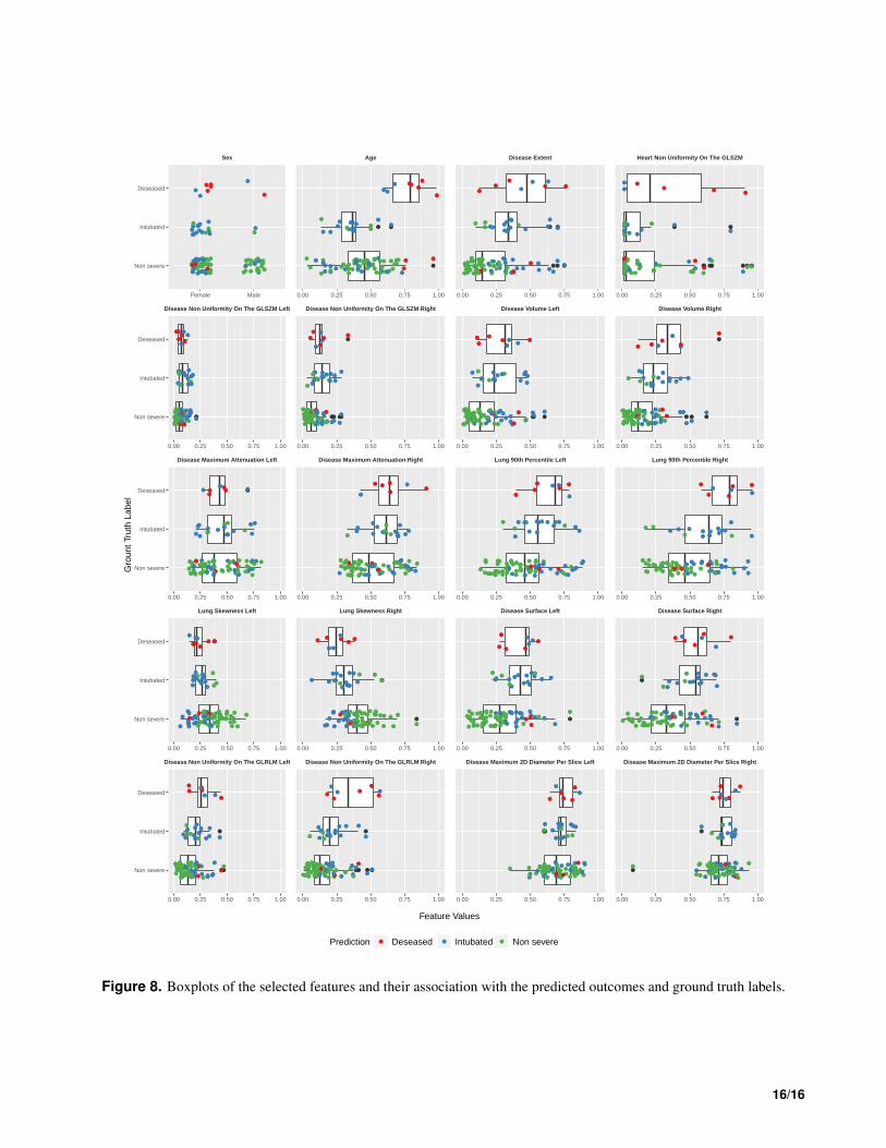
The classifiers were applied in a hierarchical way, performing first the staging and then the prognosis. More specifically, amajority voting method was applied to classify patients into severe and non-severe cases (Table 6). Then, another majorityvoting was applied on the cases predicted as severe only to classify them into intubated or deceased (Table 7). In such a setup,the correlation of the reported features are summarized in Table 5. For the hierarchical prognosis on the three classes a votingclassifier for the prediction of each class against the others has been applied to aggregate the predicted outcomes from the 7selected methods. In the Figure 8 we visualize the distributions of the different features along the ground truth labels and theprediction of the hierarchical classifier for each subject. In particular, all the samples are grouped using their ground truth labelsand a boxplot is generated for each group and each feature. Additionally, color coded points are over imposed at each boxplotdenoting the prediction label. It is therefore clearly visible that some features such as the disease extent, the age, the shape ofthe disease and the uniformity seems to be very important on separating the different subjects.

9/16

0.05

0.10

0.15

0.20

100,000 200,000 300,000Number of Batches

Loss

(W

CE

)

set

train

validation

AtlasNet 2D

0.05

0.10

0 100,000 200,000 300,000Number of Batches

Loss

(D

L) set

train

validation

U−Net 3D

Figure 6. Training and validation curves for one template of AtlasNet and the 3D U-Net.

Statistical AnalysisThe statistical analysis for the deep learning-based segmentation framework and the radiomics study was performed usingPython 3.7, Scipy35, Scikit-learn36, TensorFlow37 and Pyradiomics34 libraries. The dice similarity score (DSC)26 was calculatedto assess the similarity between the 2 manual segmentations of each CT exam of the test dataset and between manual andautomated segmentations. The DSC between manual segmentations served as reference to evaluate the similarity between theautomated and the two manual segmentations. Moreover, the Hausdorff distance was also calculated to evaluate the quality ofthe automated segmentations in a similar manner. Disease extent was calculated by dividing the volume of diseased lung by thelung volume and expressed in percentage of the total lung volume. Disease extent measurement between manual segmentationsand between automated and manual segmentations were compared using paired Student’s t-tests.

For the stratification of the dataset into the different categories, classic machine learning metrics, namely balanced accuracy,weighted precision, and weighted specificity and sensitivity were used. Moreover, the correlations between each feature and theoutcome was computing using a Pearson correlation over the entire dataset.

CT parameters between the 6 centers were compared using the analysis of variance, while patient characteristics betweentraining/validation and test datasets were compared using chi-square and Student’s t-tests.

Training/ validation dataset Testing datasetCenter A Center B Center C Center D Center E Center F

CT equipment Somatom AS+ Resolution HD Aquilion Prime Somatom Edge Revolution HD Aquilion PrimeKilovoltage 100-120 120 100-120 100-120 120-140 100-120

DLP(mGy.cm)

109±42[44-256]

306±104[123-648]

102±30[43-189]

131±44[55-499]

177±48[43-276]

115±26[75 - 186]

CTDIvol(mGy)

3.2±1.5[1.2-11.9]

8.7±2.8[3.9-18.5]

2.7±0.9[1.0-5.3]

3.2±0.9[1.4-9.5]

5.5±1.8[1.2-12.3]

2.5±0.6[1.7-4.3]

Slice thick-ness

1mm 0.625mm 1mm 0.625mm 1mm 1mm

ConvolutionKernel

i70 Lung FC51-FC52 i50 Lung FC51-FC52

Iterative re-constructions

SAFIRE 3 ASIR-v 80% IDR 3D0.67 SAFIRE 4 ASIR-v 60% IDR 3D

Table 1. Acquisition and reconstruction parameters. Note.— For quantitative variables, data are mean ± standard deviation,and numbers in brackets are the range. CT = Computed Tomography ; CTDIvol = volume Computed Tomography Dose Index ;DLP = Dose Length Product * significant difference with p < 0.001

References1. Zu, Z. Y. et al. Coronavirus disease 2019 (covid-19): a perspective from china. Radiology 200490 (2020).

10/16

Training/Validation Dataset(Centers A+B+C; N=50)

Test Dataset(Centers D+E+F; n=130) p value

Age (y) 57±17 [26-97] 59±16 [17-95] 0.363No. of Men 31(62) 87(67) 0.534Disease extent*Manual 18.1± 14.9 [0.3-68.5] 19.5±16.5 [1.1-75.7] 0.574Automated - 19.9%±17.7 [0.5-73.2] -DLP (mGy.cm) 180±124 [43-527] 139±49.0 [43-276] 0.026CTDIvol (mGy) 4.9±3.4 [1.0-13.0] 4.0±1.9 [1.2-12.3] 0.064

Table 2. Patient characteristics in the datasets used for developing the segmentation tool. Note. For quantitative variables,data are mean ± standard deviation, and numbers in brackets are the range. For qualitative variables, data are numbers ofpatients, and numbers in parentheses are percentages. CTDIvol = volume Computed Tomography Dose Index; DLP = DoseLength Product *Percentage of lung volume on CT, calculated on the full volume for the training/validation dataset and 20slices in the test dataset

Training/Validation Dataset(Centers A+B+D*; N=383)

Test Dataset(Centers C+E+F; n=95) p value

Age (y) 63±16 [24-98] 57±15 [17-97] 0.001No. of Men 255(67) 65(68) 0.732Disease extent** 19.6±17.0 [0.0-85.1] 22.5±16.4 [1.1-64.7] 0.126Short-term outcomeDeceased 19(5) 8(8)Intubated 65(17) 18(19)Alive and Not Intubated 299(78) 69(73)DLP (mGy.cm) 160±97 [44-648] 146±52.0 [ 43-276 ] 0.047CTDIvol (mGy) 4.3±2.8 [1.2-18.5] 4.1±2.0 [1.0-12.3] 0.064

Table 3. Patient characteristics in the dataset used for the developed prognosis model using radiomics. Note.— Forquantitative variables, data are mean ± standard deviation, and numbers in brackets are the range. For qualitative variables,data are numbers of patients, and numbers in parentheses are percentages. CTDIvol = volume Computed Tomography DoseIndex; DLP = Dose Length Product, ∗Enlarged by including all eligible patients over the study period, ∗∗Percentage of lungvolume on the whole CT

2. Bai, H. X. et al. Performance of radiologists in differentiating covid-19 from viral pneumonia on chest ct. Radiology200823 (2020).

3. Bernheim, A. et al. Chest ct findings in coronavirus disease-19 (covid-19): relationship to duration of infection. Radiology200463 (2020).

4. Li, K. et al. Ct image visual quantitative evaluation and clinical classification of coronavirus disease (covid-19). Eur.Radiol. 1–10 (2020).

5. Yuan, M., Yin, W., Tao, Z., Tan, W. & Hu, Y. Association of radiologic findings with mortality of patients infected with2019 novel coronavirus in wuhan, china. PLoS One 15, e0230548 (2020).

6. Truog, R. D., Mitchell, C. & Daley, G. Q. The toughest triage—allocating ventilators in a pandemic. New Engl. J. Medicine(2020).

7. White, D. B. & Lo, B. A framework for rationing ventilators and critical care beds during the covid-19 pandemic. Jama(2020).

8. Zhu, N. et al. A novel coronavirus from patients with pneumonia in china, 2019. New Engl. J. Medicine (2020).

9. Zhou, F. et al. Clinical course and risk factors for mortality of adult inpatients with covid-19 in wuhan, china: a retrospectivecohort study. The Lancet (2020).

10. Ai, T. et al. Correlation of chest ct and rt-pcr testing in coronavirus disease 2019 (covid-19) in china: a report of 1014cases. Radiology 200642 (2020).

11. Fang, Y. et al. Sensitivity of chest ct for covid-19: comparison to rt-pcr. Radiology 200432 (2020).

11/16

ClassifierBalanced Accuracy Weighted Precision Weighted Sensitivity Weighted SpecificityTraining Validation Training Validation Training Validation Training Validation

NearestNeighbors

0.66±0.02

0.55±0.03

0.88±0.01

0.73±0.03

0.85±0.01

0.78±0.01

0.47±0.03

0.32±0.04

L-SVM* 0.71±0.02

0.67±0.04

0.80±0.02

0.77±0.03

0.68±0.02

0.67±0.04

0.74±0.03

0.67±0.06

P-SVM* 0.77±0.02

0.66±0.04

0.83±0.01

0.76±0.03

0.77±0.03

0.72±0.03

0.76±0.03

0.61±0.07

S-SVM0.53±0.02

0.55±0.05

0.69±0.04

0.69±0.04

0.49±0.08

0.51±0.1

0.57±0.09

0.58±0.11

RBF-SVM* 0.74±0.02

0.67±0.06

0.82±0.01

0.77±0.04

0.66±0.02

0.63±0.06

0.81±0.02

0.71±0.08

GaussianProcess

0.63±0.03

0.59±0.04

0.82±0.02

0.77±0.04

0.83±0.01

0.80±0.02

0.43±0.04

0.38±0.05

DecisionTree*

0.78±0.02

0.68±0.04

0.85±0.01

0.78±0.03

0.69±0.03

0.64±0.05

0.87±0.03

0.72±0.08

RandomForest*

0.78±0.02

0.64±0.06

0.84±0.02

0.75±0.04

0.74±0.03

0.65±0.07

0.82±0.04

0.63±0.09

Multi-LayerPerceptron

0.83±0.04

0.58±0.03

0.90±0.02

0.72±0.02

0.9±0.02

0.73±0.03

0.77±0.06

0.43±0.05

AdaBoost* 0.8±0.03

0.63±0.03

0.86±0.01

0.75±0.03

0.76±0.07

0.66±0.07

0.83±0.08

0.6±0.11

GaussianNaive Bayes*

0.66±0.02

0.63±0.05

0.76±0.01

0.74±0.03

0.74±0.01

0.72±0.04

0.57±0.03

0.53±0.07

BernouilliNaive Bayes

0.51±0.01

0.50±0.01

0.74±0.05

0.63±0.05

0.78±0.0

0.77±0.01

0.24±0.01

0.22±0.02

QDA0.72±0.01

0.60±0.04

0.82±0.01

0.73±0.03

0.82±0.01

0.75±0.03

0.62±0.02

0.45±0.07

Table 4. Performances of the 13 evaluated classifiers. Note.— Asterixis indicates the 7 classifiers reporting a balancedaccuracy higher than 0.60 and that were finally selected, L-SVM = Support Vector Machine with a linear kernel; L-SVM =Support Vector Machine with a polynomial kernel, L-SVM = Support Vector Machine with a sigmoid kernel, RBF-SVM =Support Vector Machine with a Radial Basis Function, QDA = Quadratic Discriminant Analysis

12. Xie, X. et al. Chest ct for typical 2019-ncov pneumonia: relationship to negative rt-pcr testing. Radiology 200343 (2020).

13. Chassagnon, G., Vakalopoulou, M., Paragios, N. & Revel, M.-P. Artificial intelligence applications for thoracic imaging.Eur. J. Radiol. 123, 108774 (2020).

14. Litjens, G. et al. A survey on deep learning in medical image analysis. Med. image analysis 42, 60–88 (2017).

15. Ardila, D. et al. End-to-end lung cancer screening with three-dimensional deep learning on low-dose chest computedtomography. Nat. medicine 25, 954–961 (2019).

16. Wang, L. & Wong, A. Covid-net: A tailored deep convolutional neural network design for detection of covid-19 casesfrom chest radiography images. arXiv preprint arXiv:2003.09871 (2020).

17. Li, L. et al. Artificial intelligence distinguishes covid-19 from community acquired pneumonia on chest ct. Radiology200905 (2020).

18. Chaganti, S. et al. Quantification of tomographic patterns associated with covid-19 from chest ct. arXiv preprintarXiv:2004.01279 (2020).

19. Huang, L. et al. Serial quantitative chest ct assessment of covid-19: Deep-learning approach. Radiol. Cardiothorac.Imaging 2, e200075 (2020).

20. Jacob, J. et al. Mortality prediction in ipf: evaluation of automated computer tomographic analysis with conventionalseverity measures. Eur. Respir. J. ERJ–01011 (2016).

21. Humphries, S. M. et al. Idiopathic pulmonary fibrosis: data-driven textural analysis of extent of fibrosis at baseline and15-month follow-up. Radiology 285, 270–278 (2017).

12/16

Features CorrelationSevere vs Non Severe Intubated vs Diseased Hierarchical Classifier

Age -0.0681 0.6745 0.1853Gender -0.1517 0.0211 0.1443Disease Extent -0.3809 -0.0280 0.3491

Heartnon-uniformityon the GLSZM -0.1953 -0.0935 0.1537

Left Right Left Right Left Right

Lung Skewness 0.3324 0.3675 0.1018 -0.0229 -0.2967 -0.344790th Percentile -0.2808 -0.3221 -0.0576 0.0035 0.2526 0.3119

Disease

Maximumattenuation -0.0867 -0.1978 0.0885 0.0035 0.0958 0.1846

Surface -0.3382 -0.3289 -0.0174 0.0381 0.3034 0.3112Maximum 2Ddiameter perslice

-0.2304 -0.2236 0.1238 0.1010 0.2288 0.2183

Volume -0.3592 -0.3971 -0.0489 0.0840 0.3241 0.3863Non-uniformity

on the GLSZM-0.2944 -0.3448 -0.1379 -0.0805 0.2375 0.3004

Non-uniformityon the GLRLM -0.3280 -0.3372 -0.0219 0.0829 0.3000 0.3319

Table 5. Correlation between outcome and the 12 selected features. Note.—Note.— GLSZM =Gray level Size Zone matrix ,GLRLM = Gray level Run Length matrix

22. Vakalopoulou, M. et al. Atlasnet: Multi-atlas non-linear deep networks for medical image segmentation. In Frangi, A. F.,Schnabel, J. A., Davatzikos, C., Alberola-López, C. & Fichtinger, G. (eds.) Medical Image Computing and ComputerAssisted Intervention – MICCAI 2018, 658–666 (Springer International Publishing, Cham, 2018).

23. Anthimopoulos, M. et al. Semantic segmentation of pathological lung tissue with dilated fully convolutional networks.IEEE journal biomedical health informatics 23, 714–722 (2018).

24. Badrinarayanan, V., Kendall, A. & Cipolla, R. Segnet: A deep convolutional encoder-decoder architecture for imagesegmentation. IEEE transactions on pattern analysis machine intelligence 39, 2481–2495 (2017).

25. Çiçek, Ö., Abdulkadir, A., Lienkamp, S. S., Brox, T. & Ronneberger, O. 3d u-net: learning dense volumetric segmentationfrom sparse annotation. In International conference on medical image computing and computer-assisted intervention,

ClassifierBalancedAccuracy

WeightedPrecision

WeightedSensitivity

WeightedSpecificity

Training Test Training Test Training Test Training TestL-SVM 0.71 0.7 0.8 0.76 0.68 0.67 0.75 0.73P-SVM 0.76 0.67 0.82 0.73 0.75 0.69 0.76 0.65RBF-SVM 0.72 0.71 0.81 0.79 0.65 0.63 0.79 0.79Decision Tree 0.76 0.65 0.85 0.74 0.65 0.56 0.88 0.74Random Forest 0.76 0.7 0.82 0.76 0.71 0.65 0.8 0.75AdaBoost 0.77 0.67 0.83 0.74 0.71 0.62 0.82 0.71GaussianNaive Bayes 0.65 0.73 0.76 0.77 0.73 0.76 0.57 0.69

EnsembleClassifier 0.75 0.74 0.82 0.79 0.69 0.69 0.81 0.79

Table 6. Performances of each of the 7 individual classifiers and of the ensemble classifier to differentiate between patientwith severe and non-severe short-term outcome. Note.— L-SVM = Support Vector Machine with a linear kernel; L-SVM =Support Vector Machine with a polynomial kernel, RBF-SVM = Support Vector Machine with a Radial Basis Function kernel

13/16

ClassifierBalancedAccuracy

WeightedPrecision

WeightedSensitivity

WeightedSpecificity

Training Test Training Test Training Test Training TestL-SVM 0.84 0.78 0.87 0.84 0.81 0.85 0.87 0.72P-SVM 0.95 0.81 0.96 0.9 0.95 0.88 0.95 0.74RBF-SVM 0.9 0.62 0.92 0.83 0.90 0.77 0.9 0.48Decision Tree 0.97 0.75 0.98 0.87 0.98 0.85 0.96 0.65Random Forest 0.94 0.75 0.96 0.87 0.96 0.85 0.92 0.65AdaBoost 1 0.62 1 0.83 1 0.77 1 0.48GaussianNaive Bayes 0.82 0.75 0.86 0.87 0.83 0.85 0.8 0.65

EnsembleClassifier 0.96 0.81 0.97 0.9 0.96 0.88 0.95 0.74

Table 7. Performances of each of the 7 individual classifiers and of the ensemble classifier to differentiate between intubatedand deceased patients. Note.— L-SVM = Support Vector Machine with a linear kernel; L-SVM = Support Vector Machine witha polynomial kernel, RBF-SVM = Support Vector Machine with a Radial Basis Function kernel

424–432 (Springer, 2016).

26. Dice, L. R. Measures of the amount of ecologic association between species. Ecology 26, 297–302 (1945).

27. Sun, R. et al. A radiomics approach to assess tumour-infiltrating cd8 cells and response to anti-pd-1 or anti-pd-l1immunotherapy: an imaging biomarker, retrospective multicohort study. The Lancet Oncol. 19, 1180–1191 (2018).

28. Wang, W. et al. Detection of sars-cov-2 in different types of clinical specimens. Jama (2020).

29. CDC. Triage of suspected covid-19 patients in non-us healthcare settings. centers for disease control and prevention.https://www.cdc.gov/coronavirus/2019-ncov/hcp/non-us-settings/sop-triage-prevent-transmission.html (2020).

30. Tang, N., Li, D., Wang, X. & Sun, Z. Abnormal coagulation parameters are associated with poor prognosis in patients withnovel coronavirus pneumonia. J. Thromb. Haemostasis (2020).

31. Onder, G., Rezza, G. & Brusaferro, S. Case-fatality rate and characteristics of patients dying in relation to covid-19 in italy.Jama (2020).

32. Guo, W. et al. Diabetes is a risk factor for the progression and prognosis of covid-19. Diabetes/Metabolism Res. Rev.(2020).

33. Ferrante, E., Dokania, P. K., Marini, R. & Paragios, N. Deformable registration through learning of context-specific metricaggregation. In International Workshop on Machine Learning in Medical Imaging, 256–265 (Springer, 2017).

34. Van Griethuysen, J. J. et al. Computational radiomics system to decode the radiographic phenotype. Cancer research 77,e104–e107 (2017).

35. Virtanen, P. et al. Scipy 1.0: fundamental algorithms for scientific computing in python. Nat. methods 1–12 (2020).

36. Pedregosa, F. et al. Scikit-learn: Machine learning in python. J. machine learning research 12, 2825–2830 (2011).

37. Abadi, M. et al. Tensorflow: Large-scale machine learning on heterogeneous distributed systems. CoRR abs/1603.04467(2016). 1603.04467.

14/16

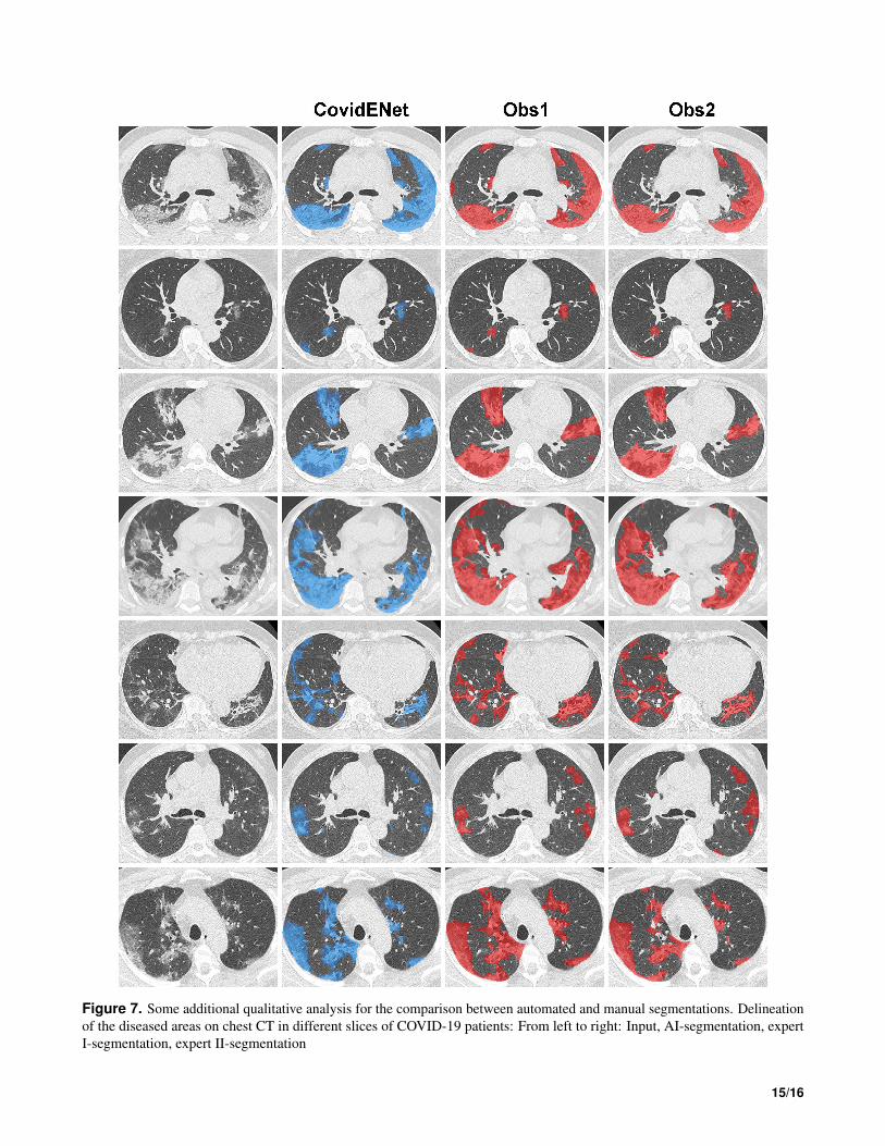
Figure 7. Some additional qualitative analysis for the comparison between automated and manual segmentations. Delineationof the diseased areas on chest CT in different slices of COVID-19 patients: From left to right: Input, AI-segmentation, expertI-segmentation, expert II-segmentation

15/16

●

●

●

●

●

●

●

●

● ●

●

●●

●

●●

●

●●●

●

●●

●

●●

●

●●

●

●

●

●●

●

●

●

●●

●

●

●

●

●

●

●●● ●

●

●

●

●●

●

●

●

● ●

●

●● ●

●

●●●

●

●

●

●

●

●

●

●

●

●●

●

●

●

●●

●

●

●

●

●●

●

●●

●

●

●

Non severe

Intubated

Deseased

Female Male

Sex

●●

●

●

●

●

●

●

●

●

●

●

●

●●

●

●●●

●

●●

●

●

● ●

●

●

●

●

●

●

●●

●

●

●●

●

●●

●

●

●

●

●

● ●●

●●

●●

●

●●

●

●

●●●

●

●●

●

●

●● ●●●

●

●

●

●

●●

●

● ●

●

●

●●

●

●

●

●

●

●

●

●

●

● ●

●

●

0.00 0.25 0.50 0.75 1.00

Age

●●

●●●

●

●

●

●

●

●

●

●

●

● ●●

●

●●

●

●

●●●

●●

●

●

●●

●●

●

●

●

●●

●●

● ●●●

●

●● ●

●

●

●●

●

●

●

●

●

●

●

●

●●

●

●

●

●●

● ●●

● ● ●

●

●

●

●

●

●

●

●

●●●

●

●

●●

●

●

●

●

● ●

●

●●

●

●

●

0.00 0.25 0.50 0.75 1.00

Disease Extent

● ●

● ●●●● ● ●

●

●

●

●

●

●

●

●●

●

●

●

●●

●●

●

●

●●● ●●

●

●

●●

●●

●

● ●●

●

●●

●

●

●

●

●●●

●

●

●●

●●

●●

●

●●

● ●● ●●

●●

●

●

●

●

●

●

●

●

● ●

●●

●

●

●

●

●

●

●

●● ●

●

0.00 0.25 0.50 0.75 1.00

Heart Non Uniformity On The GLSZM

●

●

●

●

●

●

●

●

●

●● ●●●●● ●

●

●●

●

●

●

●

●

●

●●●

●

●

●●

●

●

●● ●

●●

●

●

●

●

●

●●

●●

●

●●

●

●

●●

●

●●●

●

●

●●

●●

●

●●

●

●

●

●

●

●●

●

●●●

●

●●●

●

●

●

●

●●

●

●●●

●

●Non severe

Intubated

Deseased

0.00 0.25 0.50 0.75 1.00

Disease Non Uniformity On The GLSZM Left

●

● ●●●

●

●

●

●

●

●

●

●

●●

●

●

●●●

●

●

●● ●●

●●

●

●●

●

●●

●

●●●

●

●● ●

●

●

●

●●

●

●

●●

●

●

●

●●

●

●●

●

●

●

●

●

●

●●●●

●

●

●

●

●

●

●

●●

●

●

●

●

●●

●

●

●

●

●

●

●

●

● ●

●

●●●

●

●

0.00 0.25 0.50 0.75 1.00

Disease Non Uniformity On The GLSZM Right

● ●●

●

●

●

●

●

●

●

●

●●

●●

●●● ●

●

●● ●●

●

●

●

●

●

●●

●

●

●

●

●

●

●

●

●

●

●

●

●

● ●

●

●●

●●

●

●

●

●

●

●

●

●

●

●●

●

●

●

● ●●

●●

●●●

●

●●

●●

●

●●

●

●

●

●●

●

●

●

●

● ●

●

●●

●

●

●

0.00 0.25 0.50 0.75 1.00

Disease Volume Left

●

● ● ●

●

●

●

●

●

●

●

●

●

●●

●● ●

●

●

●

●●

●

●●

●

●

●

●●●●

●

●●●

●●

●

●

● ●

●

●

●

●

●

●

●

●

●

●

●

●

●

●

●●

●

●●

●

●

●

●●

●●

●

●●●●

●

●

●

●●

●

●

●●

●

● ●●

●

●

●

●

● ●

●

●

●●

●

●

0.00 0.25 0.50 0.75 1.00

Disease Volume Right

●●

●

●

●

●

●

●

●

●

●

●●

●

●●

●

●

●●

●●●

●

●

●●

●

●

●

●

●

●

●●

●●

●

●●

●

●

● ●

●

●●

● ●●

●

●

●

●

● ●

● ●●

●

●

●●

● ●

●

●● ●

●●

●

●

●

●

●

●

●

●●

●

●

●

●

●

●

●

●

●

●

●

●

●

●

●Non severe

Intubated

Deseased

0.00 0.25 0.50 0.75 1.00

Disease Maximum Attenuation Left

●

●

●

●

●

●

●

●

● ●●● ●

●

●●

●

●●

●

●●

●

●

●

●

●

●●

●

●

●● ●

●●

●●

●

●

●

● ●

●

●

●●●●

●

●

●

●●●

●

●●

●

●

●●●

●

●●●● ●

●

●

●

●

●●

●

●

●

●

●

●● ●

●

●

●

●

●

●●

●

●

●

●

0.00 0.25 0.50 0.75 1.00

Disease Maximum Attenuation Right

●

●

●

●

●

●

●

●

●●

●

●

●

●●

●

●

● ●●

● ●●

●

●

●

●

● ●

●

●●

●

●

●●● ●●

●

●●●

●

●●●

●●

●

●

●

●●●

●

●

●●

●

●

●●

●●

●

● ● ●

●

●

●

●

●

●

●

●●●

●

●

●

●

●

●

●

●

● ●

●

●●

●

●

●

0.00 0.25 0.50 0.75 1.00

Lung 90th Percentile Left

●

●

●

●

●

●

●

●

●

●

●

●

●

● ●

●

●

●

●

●● ●

●

●

●

●

●● ●

●

●●

●

●● ●

●

●

●

●

●●

●

●

●

●

●

●

●

● ●

●

●●

●

●●● ●

●

●●●

●

●

●

●

●●● ●

●

●●

●

●

●●

●

●

●

●

●

●

●

●

●●

●

●

●

●

●

●

0.00 0.25 0.50 0.75 1.00

Lung 90th Percentile Right

●●

●

●

●

●

●

●

●

●●

●●

●

●

●

●

●

●●

●

●●

●

●

● ●

●

●●

●

●●

●●

●●

● ●

●

●

●●

●

●

●

●

●

●

●

●●

●

●

●

●

●

●

● ●

●

●

● ●

●

●

●

●

●

● ●

●

●

●

●●

●

●●

●

●

●● ●

●

●

●

●

●

●

●

●

●●

●

●Non severe

Intubated

Deseased

0.00 0.25 0.50 0.75 1.00

Lung Skewness Left

●

●

●

●

●

●

●

●

●

●

● ●●●

●●

●●

●

● ●

●

●

●

●

●

●●

●

●

●

●

●●

●● ●●●

●

●

●

●

●

●

●

●●●

●

●

●

●

●

●●●

●

●●

●

●

●

●

●

● ●●

●

●●

●

●

●●

● ●

●

●●

●

●

●

●

●

●

●

●

●

●●

●

● ●

●

●

●

0.00 0.25 0.50 0.75 1.00

Lung Skewness Right

●

●

●

●

●

●

●

●

●

●

●

●

●●

●

●●

●

●● ●●

●●

●

●● ●

●●

●

●●

●●●

●●

●●

●

●●

●

●

● ● ●●●

●

●

●

●●

●

●

●●

●

●

●

● ●●●

●●

●

●●

●

●

●

●●

●

●

●

●

●

●●

●

●

●

●

●

●

●

●

●

●●

●

●

0.00 0.25 0.50 0.75 1.00

Disease Surface Left

●

●

●

●

●

●

●

●

●

●

●● ●

●●

●●

●

●

●●

●

●●

●

●

●●●

●●

●

●

●

●●

● ●

●● ●

●

●

●

●

●

●●

●●●

●●

●

●

●

●

●●●

●

●

●

●●

●

● ●● ●●

●

●

●●

●

●

●

●

●●

●

●●

●

●

●

●

●

●

●

●

●

●

●

●

0.00 0.25 0.50 0.75 1.00

Disease Surface Right

●

●●

●

●

●

●

●

●

●

●

●● ●

● ●

●

●

●

●

●●●

●

●

●

●

●

●

●

●

●

●

●

●

● ●

● ● ●

●●

●

●●

●

●

●●

●

●

●

●●

●

●● ●

●

●

●

●

●

●

●

●●●●

●●●●

●

●

●

●●

●

●●

●

●

●●

●

●

●

●

●

●

●

●

●

●●

●

●Non severe

Intubated

Deseased

0.00 0.25 0.50 0.75 1.00

Disease Non Uniformity On The GLRLM Left

●

● ● ●●

●

●

●

●

●

●

●

●

●●● ●

●

●●

●

●

●

●●

●●

●

●

●●● ●●

●

●●●

●

●●

●

● ●

●

●● ●

●

●

●

●

●●

●●

●

●

● ●

●

●

●●

●

●

●● ●

●

●

●

●●●

●

●●

●●

●

●

●●

●

●

●●

●

●

●

●

●

●

●

●●

●

●

●

0.00 0.25 0.50 0.75 1.00

Disease Non Uniformity On The GLRLM Right

●●

●

●

●

●

●

●

●

●

●●

●●

●●●

●

●

●

●●

●●

●

●

●

● ●●

●

●

●

●● ●●

●

●

●●

●

●

●●

●

● ●

●

●

●

●

●

●

●●

●

●

●

●

●

●

●●

● ●● ●

●●

●

●

●

●●

●

●

●

●●●

●

●● ●

●

●

●

●

●●

●

●●●

●

●

0.00 0.25 0.50 0.75 1.00

Disease Maximum 2D Diameter Per Slice Left

●

●

●

●

●

●

●

●

●

●

●●

● ●

●

●

●

●

●

●●●

●

●●

●

●

●

●

●

●

●

●

●●● ●

●●

● ●

●

●

●

●

●

●

●●

●

●

●●

●

●

●

●

●● ●●

●

●

●

●

●

●

●

●

●●

●

●

●●

● ●

●

●● ●

●

●

●●

●

●

●

●

●●

●

●

● ●

●

●

0.00 0.25 0.50 0.75 1.00

Disease Maximum 2D Diameter Per Slice Right

Feature Values

Gro

unt T

ruth

Lab

el

Prediction ● ● ●Deseased Intubated Non severe

Figure 8. Boxplots of the selected features and their association with the predicted outcomes and ground truth labels.

16/16