Embed Size (px)
Citation preview

Louisiana State UniversityLSU Digital Commons
LSU Master's Theses Graduate School
2013
Aggregation of uncontrolled fluids duringcatastrophic system failures in offshoreenvironmentsJames Thomas StiernbergLouisiana State University and Agricultural and Mechanical College, [email protected]
Follow this and additional works at: https://digitalcommons.lsu.edu/gradschool_theses
Part of the Petroleum Engineering Commons
This Thesis is brought to you for free and open access by the Graduate School at LSU Digital Commons. It has been accepted for inclusion in LSUMaster's Theses by an authorized graduate school editor of LSU Digital Commons. For more information, please contact [email protected].
Recommended CitationStiernberg, James Thomas, "Aggregation of uncontrolled fluids during catastrophic system failures in offshore environments" (2013).LSU Master's Theses. 2178.https://digitalcommons.lsu.edu/gradschool_theses/2178

AGGREGATION OF UNCONTROLLED FLUIDS DURING CATASTROPHIC SYSTEM
FAILURES IN OFFSHORE ENVIRONMENTS
A Thesis
Submitted to the Graduate Faculty of the
Louisiana State University and
Agricultural and Mechanical College
in partial fulfillment of the
requirements for the degree of
Master of Science in Petroleum Engineering
in
The Craft and Hawkins Department of Petroleum Engineering
by
James Stiernberg
B.S., The University of Texas at Austin, 2009
August 2013

ii
Acknowledgements
I would like to thank my parents for supporting me through my undergraduate studies and
always backing me up in the decisions I made. Lina Bernaola has also made a significant impact
on my life and I owe her a great deal for helping me see the completion of this work. I am
grateful to the Louisiana State University and the faculty in the Craft and Hawkins Department
of Petroleum Engineering in particular for giving me the opportunity to pick up my academic
career again after working in the field. Regarding my admission, I am indebted to those who put
their reputation on the line by vouching for me during the application process; namely, Dr.
Russell Johns, Dr. Neil Deeds, and Dr. Bayani Cardenas. I have learned a great deal from all
three and I cannot underline their contribution to my success enough.
Dr. Richard Hughes and Dr. Mayank Tyagi are inspiring instructors and dedicated advisors both
and, without their help, this work would not have been possible. I would like to extend my
gratitude towards Dr. Julius Langlinais and also Shell for financial support in this research and
my academic endeavors here at LSU. Dewayne Anderson at SPTgroup has been invaluable with
understanding OLGA®
and troubleshooting simulation errors that came up. Venu Nagineni has
been my friend and is now also my connection over at Calsep; I’m grateful for all the help he
offered me concerning PVTsim®. Finally, I’d like to thank Muhammad Zulqarnain for some
guidance during my studies as well as providing excellent pictures of real oilfield equipment.

iii
Table of Contents
Acknowledgements ......................................................................................................................... ii
List of Tables .................................................................................................................................. v
List of Figures ................................................................................................................................ vi
Nomenclature ............................................................................................................................... viii
Abstract ........................................................................................................................................... x
Chapter 1: Introduction .................................................................................................................. 1
1.1 Motivation for Research ....................................................................................................... 1 1.2 Thesis Outline ....................................................................................................................... 1
Chapter 2: Considerations and Problem Setup .............................................................................. 3 2.1 Conceptualizing the Scenario ............................................................................................... 3
2.2 Reservoirs and Fluids ........................................................................................................... 3 2.2.1 Influence of Formation Parameters ................................................................................ 4 2.2.2 Fluid Properties and Flow Performance ......................................................................... 7
2.3 Impact of Production Tubing ............................................................................................... 9 2.3.1 Installed Components ................................................................................................... 10
2.3.2 Geometry of Tubulars................................................................................................... 12 2.4 Preliminary Conclusions from Performance Relationships ............................................... 12
Chapter 3: Theory of Implemented Tools .................................................................................... 15 3.1 Nodal Analysis ................................................................................................................... 15 3.2 Simulation Software Packages OLGA
® and PVTsim
® ...................................................... 15
3.2.1 The Flow Assurance Software OLGA®
....................................................................... 17 3.2.2 Phase Behavior and PVTsim
® ...................................................................................... 19
Chapter 4: Leak Geometry and Discharge Coefficient ................................................................ 23 4.1 Sheared or Parted Pipe ....................................................................................................... 24
4.1.1 Gilbert Discharge Equation .......................................................................................... 24 4.1.2 Validity of the Gilbert Equation and Other Methods for Seafloor Leaks .................... 25
4.2 Leaking from a Failed Flange Connection ......................................................................... 29
4.3 Arbitrary Hole Shape and Modifications to the Flow Equation ......................................... 31
Chapter 5: Method and Procedure ............................................................................................... 34
5.1 OLGA® Flow Model .......................................................................................................... 34
5.2 Phase Behavior Studies ...................................................................................................... 37
Chapter 6: Discussion and Results ............................................................................................... 39 6.1 Commingling Fluids with Various Pressures ..................................................................... 39 6.2 Influence of Mixture Ratio on Fluid Properties ................................................................. 40 6.3 Compositional Effects in Simulation ................................................................................. 43

iv
6.3.1 Effect of Undersaturated Oil Coming in Contact with Condensate Gas ...................... 43
6.3.2 Estimating GOR with Heptanes Plus Fraction ............................................................. 46
Chapter 7: Conclusions ................................................................................................................ 54 7.1 Performance Relationships Dependencies ......................................................................... 54
7.2 Position and Shape of Leak ................................................................................................ 54 7.3 A New Correlation When Information is Scarce ............................................................... 55 7.4 Suggestions on Future Work .............................................................................................. 55
Bibliography ................................................................................................................................. 58
Appendix ....................................................................................................................................... 63
A. Fluid Bank ............................................................................................................................ 63 B. Heat-Transfer Coefficient Calculations ............................................................................... 65
Vita ................................................................................................................................................ 69

v
List of Tables
1 Original Reservoir Properties Used in Sensitivity Study ........................................................ 6
2 Results of TPR Sensitivity Study .......................................................................................... 12
3 Coefficients Proposed for the Gilbert Flow Equation ........................................................... 24
4 Relative Differences of Various Discharge Estimation Methods .......................................... 26
5 Liquid Rates Resulting from Different Pressures and Gas-Liquid Ratios ............................ 31
6 Ratios used in Condensate-Oil Mixtures ............................................................................... 37
7 Justification of Mixture Ratios Used in the PVT Study ........................................................ 38
8 Liquid Leak Rates (BOPD) of Condensate-Black Oil Mixtures ........................................... 43
9 Gas Leak Rates (Mcf/D) of Condensate-Black Oil Mixtures ............................................... 44
10 Gas-Liquid Ratios (ft3/bbl) from the Gas Tieback Only .................................................... 45
11 Percent Change in Gas-Liquid Ratios from Wellheads to Leak Point. .............................. 46
12 Condensate Fluids Used in Studies and Some of Their Properties .................................... 63
13 Black Oils Used in Studies and Some of Their Properties ................................................ 64
14 Well Profile and Material Properties Used in Thermal Calculations ................................ 66

vi
List of Figures
1 Schematic of Simplified Confluence and Leak Section .......................................................... 4
2 Parametric Study of Reservoir Properties. .............................................................................. 7
3 Parametric Study of Formation Fluid ...................................................................................... 8
4 Block Diagram of Iterative Solution ..................................................................................... 10
5 Parametric Study of Tubing Performance Relationship ........................................................ 11
6 Overview of Important Variables in Hydrocarbon Production ............................................. 13
7 Duns and Ros Flow Pattern Map ........................................................................................... 16
8 Examples of Sufficient and Invalid Discretizations .............................................................. 18
9 Failure Mode Tree for Deep Water Wells ............................................................................. 23
10 Discharge Model Comparisons .......................................................................................... 26
11 Choke Model as Used in OLGA®
...................................................................................... 28
12 Wellhead Flange Diagram ................................................................................................. 30
13 Examples of Flange Varieties and Connections for Subsea Applications ......................... 30
14 Arbitrary Hole Geometry in Ruptured Pipe ....................................................................... 33
15 Diagram of Gathering System as Modeled in OLGA® Simulation ................................... 35
16 Well Cross-Section Showing Dimensions of Tubulars and Cement ................................. 36
17 Gas-Liquid and Formation Volume Factor vs. Liquid Flow Rate ..................................... 40
18 Phase Diagrams for Molar Mixtures of Condensate and Black Oil ................................... 41
19 90% Quality Lines for a Condensate-Black Oil Mixture ................................................... 42
20 Gas-Liquid Ratio Sampling Points within the OLGA® Model .......................................... 45
21 Initial GOR Veresus Heavy Components Fraction ............................................................ 47

vii
22 Fitting Simulation Data to the Overall Fluid Trend ........................................................... 48
23 Comparing Various Methods for Predicting GOR ............................................................ 49
24 Drift in Heptanes-Plus Prediction While Developing Correlation .................................... 51
25 Correlation Procedure Diagram ......................................................................................... 52
26 Hierarchical Mixing ........................................................................................................... 53
27 CFD Model of Well Flange Leak Point ............................................................................. 56

viii
Nomenclature
Symbols Description SI Units Field Units
γ Euler constant = 0.5772 - -
Δ Change in some variable - -
ε Coefficient of emissivity - -
κ Specific Heat Ratio - -
μ Viscosity P or Pa·s lbm/ft·s
ρ Density kg/m3
lbm/ft3
φ Fugacity coefficient Pa psi
C Courant (CFL) number - -
CD Discharge coefficient - -
ct Total isothermal compressibility Pa-1
psi-1
g Gravitational acceleration m/s2
ft/s2
GOR/GLR Gas-oil/gas-liquid ratio m3/m
3 cf/bbl
hc Convective heat-transfer coefficient W/m2-°C Btu/ft
2-hr-°F
hr Radiative heat-transfer coefficient W/m2-°C Btu/ft
2-hr-°F
hres Reservoir thickness m ft
hti Conductive heat-transfer coefficient W/m2-°C Btu/ft
2-hr-°F
HL Liquid holdup - -
k Thermal conductivity W/m-°C Btu/ft-hr-°F
K Permeability m2 mD
N Liquid velocity number - -
Nd Diameter number - -
Nl Liquid viscosity number - -
ni Moles of species i - -
P or p Pressure N/m2
lbf/ft2
Pr Prandtl number - -
Q Volumetric Flow Rate m3/s ft
3/s
r Radius m, cm ft, inches
RN Gas velocity number - -
Re Reynolds number - -
SG Specific Gravity - -
T Time days days
u Velocity m/s ft/s
V Volume m3
ft3
x Spatial discretization length m ft
Z Compressibility factor - -

ix
Subscripts Description
ann Annulus
cem Cement
ci, co Inner and outer casing surface
p Phase
res Reservoir conditions
s Source
sep
sg
Separator conditions
Superficial gas [velocity]
sl Superficial liquid [velocity]
ti, to Inner and outer tubing surface
wf Flowing well
wh Wellhead

x
Abstract
Safety culture relating to offshore operations has shifted since the Deepwater Horizon blowout
and resulting oil spill. This incident has prompted the research of high volume spills during all
stages of hydrocarbon exploration and production. This study particularly covers the interactions
of wells and offshore networks as they pertain to situations where a release of reservoir fluids to
the environment is occurring. Primary concerns of this investigation are stream confluences, leak
modeling, and fluid behavior; the first two will be handled with various numerical software
packages (OLGA®, CFD, and nodal analyses) while the later will require more rigorous
treatment and a combination of these tools with dedicated phase behavior software (such as
PVTsim®). This research will combine with risk analysis work being done by others to identify
high-priority system failure scenarios.
The focus in modeling high-volume leaks thus far has been placed upon reservoir properties,
geology and modeling the most uncertain things when this research shows that the most
influential variables for particular reservoirs lie within the flow path. When operating offshore,
wells connect to subsea manifolds or other junctions to form unforeseen mixtures of crude oils;
these combined fluids dictate the outcome of potentially devastating releases offshore.
Flow rates through chokes have been modeled using only a few parameters, namely the pressure,
choke size and the gas-liquid ratio (GLR). The leak considered herein will choke flow and create
a back pressure, which will control how fluids move from the reservoir to wellhead. A properly
tuned equation of state can predict the GLR fairly well, but falls short when attempting to
combine the GLR of two or more fluids. A correlation is proposed to allow for more accurate
leak models when only simple fluid properties are known, such as the heptanes-plus fraction.

1
Chapter 1: Introduction
Introduction
1.1 Motivation for Research
Drilling frontiers have continuously expanded due to the demand for oil. Over 44,000 wells have
been drilled in the Gulf of Mexico since 1947 (Forrest et al., 2005) and it is in the deepest of
these wells that higher pressure and higher temperature reservoirs are typically located. Large
reservoirs can be found at such extremes, but the capital investment to discover and develop
these reservoirs is enormous and increasing. It is also costly to maintain and operate the
platforms that produce the hydrocarbons to surface. Limited slots for wells on a platform provide
an impetus to develop satellite fields, which aggregate produced fluids before allowing them to
flow to facilities at the surface. However, extending the working life of a platform in this manner
may carry unintended consequences and risks. Each node or junction in the network of flow lines
from the infrastructure beginning at the seafloor and continuing up to the platform is a possible
leak point. Knowing the rate of each fluid phase at these junctions and the duration of any leak is
essential to calculating the magnitude of the accident and predicting the environmental impact.
1.2 Thesis Outline
Presented herein are the results of simulations describing the aggregation of a number of
reservoir fluids, with varying physical and chemical properties, in a subsea development. The
goal is to model higher profile reservoirs, which would potentially be the most damaging upon
unfettered release of their energy. Of particular interest is how these reservoirs would combine at
confluences in different parts of the surface network. For instance, what happens when subsea
safety valves fail below a single template and allow low and high gravity crudes to mix? Chapter

2
two begins by setting up such a generic scenario, discussing the types of reservoirs involved and
the most important parameters responsible for pressure losses. Chapter three follows with more
in-depth theory related to the methods and tools used in the present research. Parameters
factoring into flow through a leak are discussed in chapter four. The choices of which correlation
or physical model to use is described in chapter five on the procedures carried out in this study;
the benefits and pitfalls of each item are exposed. A final discussion of the results concludes the
work and offers suggestions on how future engineering designs can benefit.

3
Chapter 2: Considerations and Problem Setup
Considerations and Problem Setup
2.1 Conceptualizing the Scenario
The primary objective of the study is to understand how multiple sources of fluid can combine
when fluid properties and flow path configurations are known. The leak, of unknown geometry
and size, constrains effluent flow at a relatively low, hydrostatic pressure; there is a difference to
consider between produced hydrocarbon and water within a pipeline versus said fluids escaping
directly to the seafloor at hydrostatic conditions. A basic scenario will be used first to investigate
the sensitivities of various parameters within the system and then an effort will be made to adjust
this to more realistic setups.
2.2 Reservoirs and Fluids
Modeling two different reservoirs, containing disparate fluids, will be sufficient for the initial
model and will provide some insight on how flow rates and void fractions are affected when
these two entities are joined. To link them, two vertical, straight-hole wells are combined
whereby their production paths are connected with a simple T-joint. A schematic of the system
with variables of particular interest is presented in Figure 1 for clarification. Specific parameters
of each reservoir will not, as it turns out, create the largest impact upon the flow rates of interest
if the only types of reservoirs considered are those that are economically producible in deepwater
fields. Relative flow rates, however, will primarily be determined by fluid properties. Well
parameters, such as tubing diameter, will remain constant during this exercise; the sensitivity
owing to the system’s plumbing will be seen thereafter.

4
1 Schematic of Simplified Confluence and Leak Section
Figure 1. Schematic of the system, showing two reservoirs’ fluids converging at simple T-joint
on seafloor and downstream leak point.
This setup provides a look at contingencies which are becoming more realistic and probable as
the frontier of deepwater drilling is expanded. The analysis of commingled flow through this
junction is intriguing because it is the key difference between producing from a conventional
offshore field versus one or more satellite fields.
2.2.1 Influence of Formation Parameters
Basic parameters, such as permeability and pressure, affect the inflow performance relationship
(IPR). The concave downward appearance of an IPR curve (found by plotting wellbore flowing
pressure against flow rate) expounds, amongst other things, the time-dependence of a well’s
productivity in a given reservoir (Walsh and Lake, 2003). However, on the time scale of a
Sea Level at
zero feet depth
Seafloor
at 5,000 feet
Black Oil
Reservoir at
15,000 feet
Condensate
Reservoir at
18,000 feet
Subsea Manifold and
Point of Fluid Mixing
Resulting Spill: GLR? API?
P > PBP
P > PDP
Condensate Gas Stream
Bg, GLR, API
Black Oil Stream
Bg, GLR, API

5
blowout, one does not expect to see much change in reservoir pressure. Thus, a study of transient
flow rates from a reservoir containing only liquid and lacking skin damage reveals the following
results (seen in Figure 2). The natural flow point is indicated by the crossing of two curves, the
IPR and the tubing performance relationship (TPR) curve, and predicts the maximum openhole
flow for those conditions. The flowing bottomhole pressure (pwf) is calculated by Equation 2.1
below (Walsh and Lake, 2003). There are actually many forms of this equation, but the one used
to be consistent with the above assumptions and requirements is
2
4ln
4 wtores
ooosciwf
rce
Kt
Kh
Bqpp
(2.1)
where K is permeability, hres is reservoir thickness, pi is initial reservoir pressure, μo is oil
viscosity, t is time, γ is the Euler constant, is porosity, ct is total isothermal compressibility, Bo
is the oil formation volume factor and rw is the radius of the well. Reservoir model 1 is the initial
trial with properties listed in Table 1 (based on values from Millheim et al., 2011). Frontier
fields, particularly those of Paleogene and Jurassic origin, are the target of this study as they pose
the most challenges and risks. They differ from the conventional Pliocene and Miocene
(commonly referred to as the Upper Tertiary) reservoirs in the Gulf of Mexico which currently
account for almost 99% of proven reserves (Millheim et al., 2011). Aside from great water
depths, reservoir complexity and quality are both problematic in comparison to the Upper
Tertiary (Payne and Sandeen, 2013); high sulfur concentration is also another matter to contend
with when safely operating these fields. Shell’s Perdido platform produces from the Paleogene
(and more specifically, Eocene-aged sands), which is known for having a high gas-oil ratio

6
(Millheim et al., 2011). Thus, it will be imperative to consider two phase flow, as it plays an
important role in this study.
Table 1. Original Reservoir Properties Used in Sensitivity Study
1 Original Reservoir Properties Used in Sensitivity Study
Initial reservoir pressure 7,000 psia Oil viscosity 5 cp
Permeability 100 mD Formation volume factor 1.1
Porosity 20% Total compressibility 10-6
psi-1
Thickness 40 ft Time 500 days
Reservoir radius 15,000 ft Wellbore radius 4 inches
Lithology type is absent from the table above and can only be inferred from the porosity and
permeability given. The pay thickness given is that of a massive bed and therefore does not
include dual porosity modeling, which may be appropriate in other cases. This base reservoir
model contains roughly 900 million stock tank barrels of oil initially. Also note that
approximately one and a half years have elapsed from the first and only well being brought
online; the inner diameter of the production tubing remains constant through out the well which
contrasts with some tapered string designs currently in use and one of the examples to be
reviewed later in Chapter 5. The remaining three reservoir models have single-parameter
variations: permeability is reduced by a factor of ten in model 2, the porosity is divided by ten in
reservoir model 3 and model 4’s pay thickness is divided by ten. The greatest change seen in
Figure 2 is the permeability reduction in model 2, which is an order of magnitude less permeable
but maintains 70% of the oil rate. Model 3 nearly overlaps the original, showing only 0.6%
reduction in oil flow rate and model 4 overlaps reservoir model 2 for a similar drop in flow rate.

7
2 Parametric Study of Reservoir Properties.
Figure 2. A Parametric Study of Reservoir Properties in a generic reservoir with three variations
on its parameters shows how much the natural flow point of the system can change. The base
case IPR results from the properties given exactly as in Table 1; the green curve represents
model 2 with a permeability that is one tenth of the base case; porosity is reduced to only 20; and
the final model’s pay thickness has been reduced tenfold.
2.2.2 Fluid Properties and Flow Performance
Focus is now placed on the black oil fluid and how its characteristics can affect the flow rate and
pressure drop within the system. A similar treatment is used in this investigation; namely, a base
case is established and then each parameter is modified one at a time.
6500
6750
7000
7250
0 2500 5000 7500 10000 12500 15000
We
llbo
re P
ress
ure
, psi
a
Oil Rate, STB/D
Reservoir Sensitivity Study
TPR Base Case IPR Permeability*0.1 Porosity*0.1 Thickness*0.1

8
3 Parametric Study of Formation Fluid
Figure 3. Comparing a generic reservoir model with four different fluids to show how the
natural flow point of the system can change. The base case curve is the original IPR; the next
IPR has an oil viscosity ten times greater than the base case; another case considered a formation
volume factor 1.8 times larger, corresponding to 2.0; and total compressibility is tested at three
magnitudes greater than the original. To assess the effects of gas-liquid ratios, a new TPR was
generated which does not intersect at all with the IPR curves, thus indicating no flow.
A black oil, of 35 °API and a bubble point gas-oil ratio of 1,000 scf/bbl, is used for all the trials.
Figure 3 displays the obvious result of gas-liquid ratio leading the parameters in influence on the
reservoir’s ability to flow; a tenfold decrease resulted in no-flow conditions. The next most
important aspect is liquid viscosity, which drops flow rate by 27% after being multiplied by ten.
Following far behind, Bo decreased flow by less than two percent when increased from 1.1 to 2.0
6500
7000
7500
8000
0 2500 5000 7500 10000 12500 15000
We
llbo
re P
ress
ure
, psi
a
Oil Rate, STB/D
Formation Fluid Sensitivity Study
TPR Base Case IPR Viscosity*10 Bo*1.8 Ct*1000 GLR*0.1

9
RB/STB and compressibility increased the produced flow by approximately 2.5% when
multiplied by a thousand.
2.3 Impact of Production Tubing
Thirdly, the conduits used in the system are isolated to show that they have the greatest control
over the pressure drop and, therefore, the relative phase rates present at the leak point. During the
produced fluid’s traverse, liquid will fall out and decrease what is known as liquid holdup (HL) in
the tubing (Hasan and Kabir, 2002). In addition to this, frictional pressure losses may liberate
more vapors from the fluid, further decreasing HL.
Changes in pressure loss with a myriad of tubing dimensions are discussed in Section 2.3.1. The
dynamic nature of the gas-oil ratio (GOR) originating from one or both of the reservoirs will be
the most intriguing aspect of the problem, because, as we just saw, it is a factor which impacts
the rate of release at the leak point very strongly. Further evidence will be presented in Chapter
4. Pressure loss through the leak may lead to choked flow and will determine backpressure,
which affects the TPR calculation in turn. Hence, an iterative process, as seen in Figure 4, will be
required when simulating. A new technique, presented in Chapter 6, will shorten calculation time
by bypassing nonessential steps, which are circled with dashed lines in the figure.
Langlinais (2013) incorporates several options for computing the TPR of a well containing at
least two phases. An oil rate must be specified in order to run the Microsoft Excel VBA routine
because the water rate and gas-liquid ratio are determined on that number. Other input required
includes production tubing inner diameter, well depth (both measured and true vertical to capture
behavior of deviated wells), fluid gravities, boundary conditions and desired correlations. The

10
latter consists of nine different models for various properties influencing the outcome of the
tubing performance relationship curve.
4 Block Diagram of Iterative Solution
Figure 4. Start at the upper left with the process of estimating the leak point pressure. Follow
through the diagram until a reasonably consistent prediction of GLR can be made, otherwise
revise the system conditions and begin with the first block again.
2.3.1 Installed Components
Casing and production tubing are essential to ensuring a safe and efficient operation in the oil
and gas business. They are also some of the most important items that engineers have complete
control over during the design phase. As such, their properties should be fully understood not
only to maximize production but also to use them safely.
The main point to be understood here is that a deeper condensate reservoir, at higher pressure,
can have a great flow potential, but still contribute less to a mixture if removed far enough and
constricted enough by a given well design. Well geometry is important in this regard, because
Is GLR different
than predicted?
No
Estimate lowest possible pressure
at leak point (i.e. hydrostatic) Finish
Use new pressure at exit node
in pipe simulation software Assess/redefine
boundary and
initial conditions
No
Use the resulting GLR
to find new ΔPLeak
Is the difference
between successive ΔPLeak
values decreasing? Extract GLR at leak from
simulation results
Yes Yes

11
multiphase flow behaves differently for vertical and horizontal pipe (Duns and Ros, 1963).
Drilling a deviated hole increases its measured depth (MD) and so it follows that extended reach
wells will suffer greater pressure losses, since there was such a profound effect owing to
increasing only the true vertical depth (TVD).
5 Parametric Study of Tubing Performance Relationship
Figure 5. Contrasting different diameters, depths and various values of pipe roughness expose
the strong influence of flow path in the well on absolute open flow. These flow potentials are
quantified in Table 2.
Switching from a 3-inch pipe to a 4.5-inch pipe, both plausible sizes for offshore wells in the
Gulf of Mexico, more than doubles daily rates. Also, within the range of the problem statement
of 15,000 and 18,000 feet of true vertical depth, there is an increase of about 170% flow rate as
6500
6750
7000
7250
7500
0 2500 5000 7500 10000 12500 15000
We
llbo
re P
ress
ure
, psi
a
Oil Rate, STB/D
Tubing Performance Sensitivity Study
IPR Diameter*1.5 Depth*1.1 Roughness*10 Base TPR

12
seen in Table 2. These two elements alone make for a variable system, especially if the fluid is
lighter and its composition engenders two phases as it nears the sea floor (volatile oil and
definitely retrograde condensates).
Table 2. Results of TPR Sensitivity Study
2 Results of TPR Sensitivity Study
TPR Modification Flow Potential
(BOPD) Change
1 Original case 8,410 -
2 Diameter increased 50% 22,650 +169.3%
3 Depth increased 10% 0 -100%
4 Pipe roughness increased tenfold 7,215 -14.2%
2.3.2 Geometry of Tubulars
Though the engineer can detail the exact specifications of tubulars used in a well, one may not
always have ideal profiles to work with. Horizontal wells exemplify this point clearly insofar as
they can be toe-up (where the bottom of the hole is not the deepest portion of the well), toe-down
(the bottom of the well is lower than the heel, below the kick-off point, of the well) or
somewhere in between. A toe-up configuration carries the obvious consequence of loading up
the heel of the well with liquid hydrocarbon or water, thereby reducing the productive
capabilities of the well. Since the immediate concern of this study is to analyze worst case
scenarios, these wells will not be given thorough treatment.
2.4 Preliminary Conclusions from Performance Relationships
Examination of each portion of the system in a blowout reveals that it is tubing constrained.
Neither geology nor formation fluid has as strong an influence on production as the conduits
used, according to Duns and Ros (1963), who break down pressure losses in hydrocarbon

13
production. They state that tubing is responsible for between 57% and 82% of the pressure loss
in petroleum systems, followed by the reservoir which accounts for 11% to 36% of losses. The
remainder of the pressure losses in the system is found in the surface lines (typically amounting
to no more than 7%). These findings are graphically represented in Figure 6 to emphasize the
lesser significance of reservoir properties and the stronger influence of GOR.
6 Overview of Important Variables in Hydrocarbon Production
Figure 6. This overview of governing variables in hydrocarbon production illustrates the skewed
level of importance away from reservoir properties and towards well properties and GOR.
The tornado chart above shows the difference in surface flow rates under the various
circumstances explored in this chapter. The base case of 8,410 barrels per day is identified by the
vertical axis, which divides the flow rate potentials between the lowest possible and the highest
reasonable. In other words, porosity was reduced by one order of magnitude (to 2% porosity) for
the smallest flow rate and adjusted to 100% for the highest as an entire order of magnitude
0 5000 10000 15000 20000 25000
Tubing Diameter
Well Depth
GOR
Permeability
Thickness
Viscosity
Pipe Roughness
Compressibility
Bo
Porosity
Flow Rate, BOPD
Flow Potential Sensitivity Analysis
Lowest Potential Highest Potential

14
greater (namely, 200% porosity) does not make physical sense. The other parameters were
handled similarly, with either practical values or one order magnitude being the constraint.
Tubing diameter far outstrips other variables with a spread of approximately 19,400 barrels of oil
per day (BOPD), followed by the well depth varying the possible flow rate by 13,600 BOPD and
then GOR giving a range of 8,400 BOPD.
An argument could be made that some of these variables have the potential to vary more than
just one order of magnitude, such as permeability which can be measured, in currently producing
reservoirs, in nanodarcys (Iwere et al., 2012) to darcys. Again, the comparison provided here is
limited to what is encountered in the deeper waters of the Gulf of Mexico and thus the base
properties are similar to those encountered in the Lower Tertiary and Jurassic formations.

15
Chapter 3: Theory of Implemented Tools
Theory of Implemented Tools
3.1 Nodal Analysis
Now a standard engineering tool for production facilities and well planning, nodal analysis
studies two sets of parameters typically grouped within either the inflow or outflow section of a
system (Hein, 1987). Gilbert (1954) proposed this method for the optimization of wells on
artificial lift, but it took some time until industry adopted it in earnest. Mach et al. (1979) took up
the mantle of nodal analysis and originally defined eight different nodes, with two additional
depending on the level of detail for surface equipment; however, the number of nodes can be
reduced to four by segmenting the system at the inflow point (reservoir pressure, rP ), the
bottomhole (Pwf), the wellhead (Pwh), and finally the separator (Psep). This approach remains an
effective teaching tool, but lacks the intricacy of a numerical simulator such as SPT Group’s Oil
and Gas Simulator (formally known as OLGA®
). The complexity of fluid behavior is also lost
without proper modeling with an equation of state, now typically handled by computer programs
like PVTsim® from Calsep.
3.2 Simulation Software Packages OLGA® and PVTsim®
Production flow simulators have been under development for decades by authors such as
Bendiksen, Malnes, Moe, and Nuland from the Institute for Energy Technology (IFE), as well as
Viggiani, Mariani, Battarra, Annunziato, and Bollettini of the Pipeline Simulation Interest Group
(PSIG). A maximum of two phases was allowed by the simulator OLGA®®
, which saw its first
operable version release in the early 1980s. It did not realize its full potential until a joint venture
of several companies (Conoco Norway, Esso Norge, Mobil Exploration Norway, Norsk Hydro

16
A/S, Petro Canada, Saga Petroleum, Statoil and Texaco Exploration Norway under the SINTEF
banner) pooled their resources (Bendiksen, 1991). This development brought together several
empirical correlations into a single system. It still relies upon flow regime maps, but integrates
them with a more concrete understanding of physics. One organization of regimes, provided in
Figure 7, shows how Duns and Ros (1963) defined vertical two-phase flow.
Two-Phase Vertical Flow Regimes According to Duns and Ros
7 Duns and Ros Flow Pattern Map
Figure 7. Flow pattern map, after Duns and Ros (1963), defines regions of fluid flow for which
appropriate frictional loss correlations should be used.
The dimensionless liquid velocity number, N, and dimensionless gas velocity number, RN, are
defined by equations 3.1 and 3.2, respectively. These governing groups take into account the
Slug Flow
Mist Flow
N
RN
Bubble Flow
Plug Flow
Froth Flow
Hea
din
g
Tra
nsi
tion
Slug Flow
Mist Flow

17
superficial velocity, νs, liquid density, ρl, gravity, g, and the interfacial tension, σ, between the
two phases present.
4
gvN l
sl (3.1)
4
gvRN l
sg (3.2)
It is important to note that these numbers were established in a study that dealt with mixtures of
oil and gas with no water present. Interfacial tension is incorporated in both numbers to allow the
use of the Duns and Ros (1963) method with low concentrations of water, however the formation
of stable oil-water emulsions causes the correlation to break down when predicting frictional
pressure losses in vertical flow. Pressure losses in water and gas mixtures can also be assessed
with practical (Duns and Ros, 1963) accuracy, but will not yield comparable results to those of
oil-gas systems. Thus, it is safe to use these groups in the present deepwater system as the
flowing pressure at the leak will generally exceed hydrostatic pressure.
3.2.1 The Flow Assurance Software OLGA®
OLGA® divides flow types into two regimes: separated flow and distributed flow. The former
contains stratified and annular flow behavior, while the latter describes dispersed bubble flow
and hydrodynamic slug flow. The most important metric for determining which of these exists is
the slip, which is a ratio of average gas velocity to average liquid velocity (OLGA®, 2012). Once
determined, this information can be fed into a system of equations (ranging from a few equations
for a simple system to seven or more) for a one-dimensional simulation; typically though, five
mass conservation equations, three momentum equations and one energy conservation equation

18
are coupled with transfer equations in the dynamic three-phase flow simulations computed by
OLGA® (Anderson, 2012). All of these are limited spatially and by time step according to the
accuracy required and the Courant number (also known as the Courant, Friedrichs and Lewy
number or CFL). A general guideline for node lengths (Δxi) is given in the OLGA® user manual
(2012) and represented in equation 3.3 below; it concerns the accuracy of the representation of
the partial differential equation being solved.
22
1
1
i
i
x
x (3.3)
This also implies that each pipe should have at least two sections, but the likelihood is that pipes
will have several sections to honor the profile of a well or topography of a pipeline network. This
discussion on numerical stability and accuracy is important to the modeling of the choke in
OLGA® (see Figure 11 in Chapter 4 for the cross-section investigated). Courant, Friedrichs and
Lewy determined that the step size of the spatial and temporal variables in the numerical solution
of a partial differential equation control the stability of the finite-difference representation of the
physical system (Courant et al., 1967 and Tannehill et al., 1997). This is visualized in Figure 8
with an invalid and valid example using the velocity of a particle inside a conduit.
8 Examples of Sufficient and Invalid Discretizations
Figure 8. The Courant number ensures stability within this explicit time marching scheme. Both
simulations use the same time step (Δt), but the gridding of pipe a is too fine. A fluid particle
may travel further than the resolution (Δxa) in this case, whereas Δxb is properly sized to preclude
numerical instability in the simulation.
1 2 3
Δxb
1 2 3 4 5
Δxa
t0
t0 + Δt

19
Trefethen (1996) mentions that the amount of time progressed per step must be short enough so
that no spatial discretization is skipped during computation.
maxCx
tuC
(3.4)
It should also be noted that the approach to numerically integrating flow is decoupled vis-à-vis
temperature, which normally contributes a ±15% error (OLGA®, 2012); there is a hard-coded
correction built into the software to address this issue. Thermal considerations are minimal in
this work as the fluids flow quickly through the pipe to the seafloor and are therefore subject to
little heat loss until passing through the leak.
Boundary conditions required by the program include temperature, GLR, and pressure or flow
rate at inlets and outlets. The temperature and pressure are crucial as a number of intensive
properties are computed with them. PVTsim®, the phase behavior software discussed in the next
section, supplies tabulated information on the fluids to be used in the simulation; any value not
present in the simulation data file is interpolated from the tabulated information. Concerning
rheology, OLGA® assumes the flowing fluids to be Newtonian for basic calculations and uses
empirical correlations, available in sub-modules, to handle non-Newtonian fluids. The manner in
which a liquid or gas behaves at turns, bends and other obstructions must be approximated
through coefficients by the user. Improvements on these discharge coefficients may be
obtainable from detailed computational fluid dynamic (CFD) studies.
3.2.2 Phase Behavior and PVTsim®
J.D. van der Waals proposed an equation of state in 1873 to reflect the behavior of real fluids,
specifically the attraction between their constituent molecules and the volume each molecule

20
occupies (McCain, 1990). However, this equation is valid only at low pressures, which restricts
its application mainly to liquids and low-pressure gases (McCain, 1990). Equation 3.3 expresses
the van der Waals relationship in cubic form.
023
p
abV
p
aV
p
RTbV MMM (3.5)
Attractive forces are denoted by the constant a which corrects for pressure by an amount of
a/VM2 when added to an unadjusted system pressure. The volume occupied by molecules is
introduced via the constant b; both a and b are specific to a given fluid. The term VM is molar
volume and R represents the universal gas constant in whichever form is appropriate to the units
being used. A host of equations of state followed in this vein, but, according to McCain (1990),
the most noteworthy came from Redlich and Kwong in 1949 (with a modification later offered
by Soave in 1972) and Peng and Robinson in 1976. These are known as the SRK and PR
equations of state, respectively. Peneloux et al. (1982) stated that the SRK equation of state gives
reasonable results for pure components with low values for the acentric factor, like methane.
They refined the SRK expression with a volume correcting constant, which enhances the
predictions of liquid density at the cost of requiring another fluid parameter beyond critical
properties and the acentric factor (Riazi and Mansoori, 1992). PVTsim®
provides the option of
using either the SRK or the PR equation of state with the static or temperature-dependent version
of the Peneloux volume correction, often denoted by the letter c. In the present study, the SRK
equation of state is used with the Peneloux correction.
Mixing is of primary interest in the current study, an explanation of the insufficiency of classical
mixing rules is required. Water is a polar molecule and when paired with one other nonpolar

21
component (such as any hydrocarbon), the classical mixing rules fail to provide a reasonable
value for attractive forces, the a parameter (PVTsim®, 2012). This disparity in charge tends to
layer by component type (i.e. alternating polar and nonpolar zones of molecules) and therefore
create a structure in the mixture (Pedersen and Milter, 2004). By default, the Huron and Vidal
(H&V) rule of 1979 is employed to combat this situation in scenarios involving not only water,
but salts and hydrate inhibitors (PVTsim®, 2012). High pressure, high temperature cases are of
particular interest in this study since deepwater wells typically have both elevated reservoir
pressures and reservoir temperatures. Pedersen and Milter (2004) surveyed the effectiveness of
the H&V correction and the Cubic Plus Association (CPA) model when applied to gas
condensates, which have a significant amount of gas in the water phase. The variations
incorporated in these schemes need not be applied universally; most binary interaction
parameters (hydrocarbon-hydrocarbon pairs namely) can be calculated with the classical mixing
rule while others involving water, methanol, and others can be treated by the H&V or CPA
exception. Within the 35°C to 200°C range and 700 bar to 1000 bar window, the predictions
using H&V proved satisfactory.
Simulating multiple phases requires that fugacity, or effective pressure, be considered.
Accurately describing PVT behavior for a gas that is real requires the matching of its chemical
potential at a specified temperature and pressure with an ideal gas at the same temperature, but
different pressure. Although this chemical potential, or partial molar free energy, is not typically
expended during normal (non-flaring) production or blowouts, it does relate to phase changes
(Job and Herrmann, 2006) that often occur between bottomhole conditions and manifolds or
platforms. In the presence of equilibrated vapor and liquid, fugacity and chemical potential are
equal in both phases. The general expression of fugacity is

22
V
nVTi
i ZdVV
RT
n
P
RTln
1ln
,,
(3.6)
where ni represents the moles of component i and Z is the compressibility factor (PVTsim®,
2012). The use of fugacity allows for better accuracy in predicting equilibrium at greater
pressures, which will be encountered in any oil or gas well. Once two phases equilibrate then the
composition for each can be calculated. Thus, the relative amounts of each phase and their
physical properties used in flow calculations can be generated. These calculations must be made
along the entire flow path of each reservoir fluid in this study, because a great deal of change can
occur in the fluids before they interact with each other. The literature and software available now
adequately predict these changes up until the point of mixing.
PVTsim® incorporates a mixing scheme called allocation after the process that Pedersen (2005)
describes. The module requires molar composition of each feed stream, each stream’s volumetric
flow rate at specific pressure and temperature, and the “process plant” configuration in order to
compute the contributions provided from all sources. To do so, PVTsim® breaks down the
composition of each fluid into common discrete components and pseudocomponents. Those
components deemed necessary are created on the basis of mass flow rate entering the process
plant. Converting the volumetric rates to molar rates is accomplished assuming complete mixing
for the given pressure and temperature given. The results of these allocation computations often
do no better than other means of simulating as Chapter 6 describes. This study picks up here and
establishes a similar process based upon flow rates, but only using the heptanes-plus
pseudocomponent in the correlation. Again, the focus is producing consistent gas-oil ratios for
use in flow rate equations where information is limited.

23
Chapter 4: Leak Geometry and Discharge Coefficient
Leak Geometry and Discharge Coefficient
Before discussing the tools and processes used in this study, the leak itself must be described in
finer detail. So far the leak has been regarded as an arbitrary back pressure on a system of
converging well streams. This is essentially true, but calculating that resistance to flow becomes
a challenge when considering the types of leaks possible in deep water operations. Nichol and
Kariyawasam (2000) analyzed the risks associated with neglecting wells and, even though the
present study does not assume wells to be temporarily abandoned or shut-in, the failure mode
analysis provides insight on weak points in offshore production.
9 Failure Mode Tree for Deep Water Wells
Figure 9. The final consequence of a blowout is located at the top of this failure mode tree with
some possible fault mechanisms listed in the branches beneath it.
The type of leak geometry can vary depending on the cause described in Figure 9 and any
backup safety measures downstream of the leak. The items closest to the top are nearer to the
spill and are likely to have leaks of greater area and thus higher flow directly to the seafloor.
Leak to environment
Leak through x-mas tree Leak through tree flange
Leak through tubing
above SSSV
Leak through
production casing
flange connection
Leak through
annulus valve
Leak through
production
casing riser
Leak through surface
casing flanged connection
Leak through surface
casing annulus valve
Leak through SSSV

24
4.1 Sheared or Parted Pipe
Perhaps the worst case scenario for a subsea blowout is when a conduit, whether it is production
tubing or seafloor flow lines, breaks open entirely. Hurricanes can generate tremendous force,
which break sediment loose near production platforms, ultimately resulting in mudslides. When
hurricane Camille hit the Gulf of Mexico with nearly 70-foot high waves in 1969, such
deformation occurred in the South Pass Block 70. One platform was destroyed entirely and
another experienced a great deal of damage (Nodine et al., 2006).
4.1.1 Gilbert Discharge Equation
The risk of shearing a pipe in this fashion will not be an issue in deep waters, but other ruptures
exposing the full diameter of a flow line would certainly cause the greatest amount of
environmental damage. This type of leak has been discussed at length in the literature and one of
the most enduring models for such a scenario was initially proposed by Gilbert (1954).
C
A
LGORB
dPQ
64 (4.1)
The liquid rate, QL, is estimated with pressure, P, the opening diameter, d64, and the gas-oil ratio.
The constants A, B and C are the subject of several papers as seen in Table 3.
Table 3. Coefficients Proposed for the Gilbert Flow Equation.
3 Coefficients Proposed for the Gilbert Flow Equation
Coefficients
Correlation Author A B C
Gilbert (1954) 1.89 10.01 0.546
Baxendell (1957) 1.93 9.56 0.546
Ros (1959) 2 17.4 0.5
Pilehvari (1980) 2.11 46.67 0.313

25
Equation 4.1 is attractive because of its ease of use; the pressure can be estimated at hydrostatic,
the inner diameter of the burst pipe is known and the GOR is known for each well stream
contributing to the leak. The way these GORs combine is left for a later discussion in the results,
but may be correlated to give an approximation of flow using Gilbert’s correlation.
However, a number of limitations exist on this correlation, because it was developed for a
specific oilfield and set of pipe and valve diameters. Gilbert (1954) sampled the Ten Section
Field in the San Joaquin Valley in Kern County, California. It was this context that provided the
tubing size to be no more than 3 ½ inches inner diameter, the GLR is between 2,000 and 500,000
scf/stb, API gravity of 25-40 degrees for the oil and an upper limit of an inch for the bean (a
colloquialism for orifice) size. The relationship was initially intended to aid gas-lift design for
the area, which was the first production in the valley after seismic surveys discovered the
potential in the 1930s (Lietz, 1949). It is understood that this tool is meant for mature onshore
fields, but should apply equally well to the case presented herein if the above parameters are kept
within a reasonable range of the correlation and that the flow through the leak is choked.
4.1.2 Validity of the Gilbert Equation and Other Methods for Seafloor Leaks
To ensure that Equation 4.1 is applicable to the present study, data is collected from Ashford
(1974) and reproduced with new calculations in Figure 10 and Table 4. In Gilbert’s study (1954),
it is assumed that flow through the bean is supersonic and that upstream pressure is at least 70%
greater than pressure downstream of the restriction (thereby ensuring choked flow).

26
10 Discharge Model Comparisons
Figure 10. Existing models from the literature are tested against a data set from Ashford (1974)
to confirm their validity next to the OLGA® models being considered.
Table 4. Relative Differences of Various Discharge Estimation Methods
4 Relative Differences of Various Discharge Estimation Methods
Well d64 R P1 T1 γoil Measured
Qo
Ashford Gilbert &
Baxendell
OLGA®
model
OLGA®
with CD
(-) (-) (scf/STB) (psia) (°F) (H2O=1) (bbl/D) (%) (%) (%) (%)
1 32 1065 485 120 0.844 1010 -10.89 -10.26 -42.62 -1.69
16 1065 505 120 0.844 230 -0.43 7.68 -33.91 13.29
2
32 180 325 120 0.885 1505 -1.86 6.52 -51.91 15.99
24 180 465 120 0.885 1190 -4.03 10.63 97.92 31.07
16 173 665 120 0.885 720 -2.22 22.18 -36.41 72.72
3
32 363 425 120 0.867 1340 3.88 6.67 -45.36 18.88
24 337 575 120 0.867 1055 2.18 9.57 1579.54 30.61
16 341 775 120 0.867 590 4.75 19.97 2797.80 52.22
4
32 118 375 120 0.883 2088 -5.32 11.57 -54.49 108.23
24 107 525 120 0.883 1752 -13.47 12.70 1212.39 57.09
16 108 740 120 0.883 1068 -17.88 18.55 -43.87 35.38
5
32 127 100 120 0.882 370 55.68 61.29 -70.16 50.53
24 120 125 120 0.882 350 17.71 26.17 1722.94 17.26
16 102 225 120 0.882 290 15.86 36.96 2127.63 36.99
0
500
1000
1500
2000
2500
0 500 1000 1500 2000 2500
Cal
cula
ted
Qo
, [b
pd
]
Measure Qo, [bpd]
Discharge Model Comparisons
Ashford (1974)
Gilbert (1954) Equation
OLGA with Cd
OLGA-Modeled Leak
Linear (10% from actual)
Linear (Actual)

27
Ros (1961) describes critical flow criterion through a choke simply when the ratio of
downstream pressure to upstream pressure is 0.544. Extrapolating this to systems with different
parameters creates errors, which can be mitigated through the use of discharge coefficients (CD)
according to Ashford (1974). This term is incorporated to absorb irreversible losses not predicted
by the Bernoulli equation (Ajienka et al., 1994, Rahman et al., 2009). The calculations from
Ashford (1974) in Table 4 use values for CD ranging between 0.642 and 1.218 from the process
outlined in the same paper. To perform this calculation, the Z-factor must first be evaluated from
lab measurements as reasonably as possible (gas composition can be erratic and cause problems
in some instances, so an average may be necessary). Inserting this number into Equation 4.2
allows the liquid flow rate to be calculated. The resulting flow rate is, of course, theoretical and
must be compared to the actual rate observed; their difference, in the ratio form of qL-measured
to qL-predicted, will be the discharge coefficient.
wowogLS
wowoSgLS
woo
LSGFRSGSGRRZT
SGFRSGSGRRZT
FB
pdQ
000217.0111)(
000217.0151)(53.1
111
21
111
21
1
2
64
(4.2)
All quantities used are measured in field units. The complexity of Equation 4.2 is reduced
considerably by removing the water-oil ratio (Fwo) for cases not involving water. SG denotes the
specific gravity, whether it be for the liquid, vapor or water phase. All other definitions remain
the same as previously described or industry-accepted, such as the gas compressibility (Z), gas-
oil ratio (R) and solution gas-oil ratio (RS). Again, the CD is a ratio (refer to Equation 4.3) of the
measured to calculated and thus expected to be less than unity.
predictedL
measuredL
DQ
QC
,
, (4.3)

28
The “Gilbert & Baxendell” column contains results from Equation 4.1 using the Baxendell
coefficients. The simulation software OLGA®, to be discussed in more detail within Chapter 5, is
used to predict flow in two ways. The first, “OLGA®-model,” describes a conduit that tapers
down to the size of the orifice being studied. Simulating abrupt changes in pipe diameter is
difficult, because it creates problems when the software’s solving routine attempts to converge
on a solution. A 16/64” venturi-style choke is modeled in OLGA® in a manner as seen in Figure
11. However, OLGA®
can also use correlations with a suggested (but changeable) CD of 0.84 to
provide much more accurate results. As mentioned before, Ashford (1974) used several values of
CD while the “OLGA®
with CD” model uses only the default discharge coefficient. The CD works
best in the ½-inch case (three out of the five scenarios) and suggests a lower value for smaller
chokes.
11 Choke Model as Used in OLGA
®
Figure 11. The pipe geometry in OLGA® must be tapered gradually to prevent the software from
crashing during simulation runs. This results in very erroneous results and provides the
motivation to further study leaks with a proper CFD package that analyzes three dimensions.
-2.5
-2
-1.5
-1
-0.5
0
0.5
1
1.5
2
2.5
0 20 40 60 80 100 120
Pip
e D
iam
ete
r, [
inch
es]
Pipeline Profile, [inches]
Choke Model as Used in OLGA®

29
4.2 Leaking from a Failed Flange Connection
Another type of leak geometry that could be encountered is around the wellhead or where any
pipes mate with the aid of flanges. There are different types of connections with advantages and
disadvantages for the kind of element used between flange faces. In a basic flange, a groove is
cut into the face of the flange with a particular profile wherein a gasket sits. Reusable types of
gaskets are typically made of rubber, but they do not provide adequate containment for high
pressure fluids. Metal gaskets, or O-rings as they are sometimes called, can seal at higher
temperatures and pressures than rubber counterparts. However, the metal rings actually deform
during the process of tightening the flange bolts to provide the stronger seal, so they cannot be
used more than once. The failure of either ring can, of course, vary between a trickle to
completely eroded rings where fluid can escape via the flange-face grooves.
Deep water wells are considerably more complex than implied by the wellhead schematic in
Figure 12. However, the diagram underlines the importance of the gasket that completes the
flange connection since these flange connections are used throughout the subsea equipment (see
Figure 13) as well as the well casings. Figure 12 shows how it may come under the influence of
two different zones in the case of bad cement jobs or other minute leak paths.

30
Lock-down screw
Casing liner
Upper spool to hang liner
Flange bolt
Metal gasket, possible weak point
Lock-down screw
Second casing landed in bowl
Surface casing
Mudline
12 Wellhead Flange Diagram
Figure 12. This cross-section of a typical wellhead details common components and highlights
the gasket as the most plausible location of failure. The surface casing is likely not to fail where
it is connected to the lower flange, because it is welded (joint not explicitly shown).
13 Examples of Flange Varieties and Connections for Subsea Applications
Figure 13. Well containment warehouses are being stocked so emergency responders can react
to blowouts with the right equipment in a timely fashion. Depending on the function and pressure
rating, flanges may have a few thick bolts or several of them evenly spaced out. Photographs
were taken by Muhammad Zulqarnain while on tour at the Marine Well Containment Company’s
facility in Houston, Texas.

31
4.3 Arbitrary Hole Shape and Modifications to the Flow Equation
In the case of parted tubing, an irregular hole may manifest and create complex fluid paths for
hydrocarbon spills. After rearranging Equation 4.1 to isolate pressure, a discharge coefficient can
be applied in order to adapt the Gilbert equation to reflect the nature of the leak. Figure 14
displays a generic conduit with an oddly shaped hole in the side. Dotted lines partition the leak
off by flow behavior: the N denotes for nozzle and infers a jetting action as fluids are accelerated
through the narrower opening and the D stands for diffuser because these areas are likely to see a
slower velocity as fluid has relatively more freedom to expand in these sections. If partitioned
properly, then each of these zones could be calculated separately with their own discharge
coefficient. Compiling the results of these sections afterward could potentially improve the
results of Equation 4.1 and overall simulations in software such as OLGA®
. The importance of
these discharge coefficients can be seen in Table 5, which shows liquid discharge within several
cases. These trials were run in OLGA®
using the proper discharge coefficient for each bean size
(and not attempting to specifically model the choke within the geometry editor) to find the liquid
flow rate through a 3 ½” pipe and then Equation 4.1 was used to predict these same rates.
Table 5. Liquid Rates (MBPD) Resulting from Different Pressures and Gas-Liquid Ratios
5 Liquid Rates Resulting from Different Pressures and Gas-Liquid Ratios
GOR
OLGA® Gilbert OLGA
® Gilbert OLGA
® Gilbert
4,000 scf/stb 29 14 19 22 38 35
1,000 scf/stb 36 21 41 44 51 56
500 scf/stb 38 30 45 36 57 79
Noncritical Flow Sonic Flow Sonic Flow
3,500 psia 4,000 psia 5,000 psia
Upstream Pressure

32
Fluid flow was constrained in these trials by first holding upstream pressure constant and varying
the gas-oil ratio and then increasing upstream pressure by 600 psia and using the same GOR
values. The hypothesis here was that the two methods would, at the very least, behave in a
similar fashion if no firm agreement could be made on exact liquid flow rates. Note the lower
pressure trials at 2,400 psia and how the liquid rate drops as a consequence of increased GOR.
However, the OLGA®
simulation calculates a drop of about 11.5% in liquid flow rate whereas
the Gilbert equation shows a decrease of 37.1% in liquid flow rate. Considering the higher 3,000
psia scenarios, the result is reversed; liquid rates increase with the GOR. At these larger
pressures, the flow becomes critical and the Gilbert equation must be substituted for another
designed to deal with such conditions. Equation 4.4, proposed by Wallis (1969), is used to verify
if the multiphase flow is, in fact, critical.
2*2**
LL
L
gg
g
ggLLVV
V
(4.4)
The asterisk denotes critical flow for the overall fluid or the phase-specific flows. The in situ
volume fractions, λg and λL, are generated with the OLGA® simulation just before the leak point.
The critical fluid velocity differs for each phase however and must be computed with equations
4.5 and 4.6 below.
C
VL
1.68* (4.5)
g
g
ZTV
4.41*
(4.6)

33
The parameters, such as the gas specific heat ratio (κ), the liquid compressibility factor (C), the
gas compressibility (Z) and specific gravity of the gas (γg) are calculated with PVTsim®. Also,
the temperature (T) is input with units of Rankine. Carrying out these operations indicates that
the flow is indeed critical and provides the rates seen in Table 5.
Finally, Chapter 7 concludes with remarks about future work in this area, which may be
improved with increased understanding of flow through various hole shapes. One tool of primary
interest is CFD because it can visualize the streamline paths as fluid moves through a leak or
restriction of abnormal geometry.
14 Arbitrary Hole Geometry in Ruptured Pipe
Figure 14. The arbitrary shape of a ruptured pipe may not exhibit simple flow paths, which
complicates the computation of flow rate or pressure at that point. Converging and diverging
streamlines can affect the fluid behavior at the effluent end of the system in unknown ways.
N D D N D
Q
2
Q3
Q4
Q5
Q1

34
Chapter 5: Method and Procedure
Method and Procedure
A bank of modeled fluids was created, with details on compositions and saturation pressure
types, from various sources (Ali and McCain, 2007 and El-Banbi, Fattah and Sayyouh, 2006).
Additional modeled samples were developed from these in order to understand subtle nuances of
compositional influence on a particular feature.
5.1 OLGA® Flow Model
Two vertical wells join together at the seafloor via 25-foot long tiebacks in the model per the
problem statement in Chapter 2. Fluid flows from these tiebacks into a vertical length of pipe
open to the sea. For simplicity, the profiles of the wells are identical, reaching down to 10,000
feet true vertical depth with a deviation starting at 8,000 feet. The deviation builds at
approximately 3.5° per 100 feet. A schematic of the entire system as seen in OLGA® is displayed
in Figure 15. The wells are constructed in two main parts, an upper portion and a lower one; the
main differences between the two is the internal diameter of the production tubing increases from
4-½” in the lower part to 5-½” in the upper. To model the outlet to the sea floor a hydrostatic
pressure of 2,200 psia is applied to the leak point. This is approximately the equivalent of 5,000
feet of sea water depth. The pressure will be greater than this as the leak will impart a pressure
loss contingent upon its shape and the type fluids passing through it. Fluids exiting through this
hole are assumed to be gas and oil only for modeling simplicity; the inclusion of water bears
little significance, because most correlations for flow through an orifice do not distinguish
different liquid phases. Additional complexity in the flow paths and the fluids can be handled by

35
the software, but also adds a layer of complexity to the analysis of the results that was deemed
unnecessary.
15 Diagram of Gathering System as Modeled in OLGA
® Simulation
Figure 15. Two identical wells produce disparate fluids from unconnected reservoirs. All
pertinent features of the wells and their associated boundary conditions, such as heat transfer
coefficients, are equivalent to reduce extraneous parameters.
A great deal of consideration is given to the flow rates used under a variety of pressure
conditions, but phase behavior also relies upon system temperature. This facet of the problem is
underlined by the fact that hydrocarbons would escape to a relatively cold environment in
deepwater environments. Therefore, heat-transfer coefficients are applied to the wells, pipelines
and manifold. Heat moves through the system in different ways, so different definitions exist for
the coefficients. Formation temperature increases with depth; that heat first penetrates the cement
and the casing string it holds in place before traversing the annulus containing completion brines.

36
The dimensions of these items for both the upper section and the lower section of the well are
seen in Figure 16.
Concrete, 1”
Casing, ½”
Completion Fluid, 2” or 4 ¾”
Tubing, ½”
16 Well Cross-Section Showing Dimensions of Tubulars and Cement
Figure 16. The physical properties of the tubing, casing, brine and cement are the same for both
well sections except for the thickness of the annulus; a smaller liner is used at the bottom.
The barriers to heat transfer are in series and this leads to the form of Equation 4.3 for the overall
heat-transfer coefficient, Uto, appearing similar to electric resistances in series.
cem
rr
to
c
rr
to
CompFluid
rr
to
rcci
to
t
rr
to
toti
to
to k
r
k
r
k
r
hhr
r
k
r
hr
r
U
co
cem
ci
co
to
ci
ti
to lnlnln
)(
ln1
(4.3)
Units are consistent for Uto to have units of Btu/(hr-ft2-°F); r denotes radius measured from the
center of the production tubing, the k variables refer to heat conductivity and the h variables to
specific heat-transfer coefficients (the subscript r is for radiative heat transfer and c for
convective heat transfer). The terms are arranged to describe the resistance from the center
outward. Subscripts i and o stand for inner and outer, respectively; t is used for tubing; c for
casing; and cem for cement. This coefficient relies on a temperature gradient, so it must be
calculated along the entire well profile to couple properly with the changing formation
temperature (the geothermal gradient). A thorough discussion of calculations and example values
are provided in Appendix B.

37
5.2 Phase Behavior Studies
Using PVTsim®, trends can be developed by uniformly modifying mixing ratios between two
representative fluids of condensate gas and black oil. Molar mixtures are simply sums of two
fluids, which is to say that mole fractions of a given component are added to the mole fraction of
the same component in another fluid and then the whole mixture is normalized to one mole of
substance. Ratios are defined with the lighter fluid first, so a 9:1 mixture is nine times more
concentrated in the lighter fluid than the heavier; here, a gas condensate is mixed with black oil.
Therefore, a mixture of 9:1 is within ten percent of the original condensate’s composition and a
100:1 mixture would be within one percent of the original lighter-fluid’s composition. Mixtures
studied were varied per the scheme found in Table 6. These weightings inevitably drag the
critical points of the mixture towards the main contributing fluid’s original critical point.
Table 6. Ratios used in Condensate-Oil Mixtures
6 Ratios used in Condensate-Oil Mixtures
Fluid 1 2 3 4 5 6 7 8 9 10 11
Ratio 100:1 50:1 9:1 8:2 7:3 6:4 1:1 4:6 3:7 2:8 1:9
Originally, only the ratios between 9:1 and 1:9 were considered, but investigating the differences
of a few keys properties for larger ratios warranted the inclusion of the lower gravity mixtures
here. Notice that the first two ratios are spread much more widely than all of the other mixture
ratios in the table. The addition of the black oil, even at only 10%, has a marked effect on the
properties of the combined fluids. The converse, however, is not true as seen in Table 7, which
contains the critical properties and total density of the resulting fluids. Starting on the left side,
the lightest mixture is created with 100 parts condensate and one part black oil. Two intermediate
ratios, 50:1 and 20:1, follow before the 9:1 ratio.

38
The right side of the table displays the higher gravity mixtures, modified in the same proportions.
The relative change between the 9:1 mix and the lighter fluids as well as the relative change
between the 1:9 and the heavy mixtures are tabulated for the three parameters considered.
Table 7. Justification of Mixture Ratios Used in the PVT Study
7 Justification of Mixture Ratios Used in the PVT Study
Mixture ratios (light fluid : heavy fluid)
100:1 50:1 20:1 9:1 1:9 1:20 1:50 1:100
Critical
Presssure, psia
4873 5033 5270 5232 1651 1557 1510 1494
-6.9% -3.8% 0.7% - - -5.7% -8.6% -9.5%
Critical
Temperature,
°F
135.91 167.21 245.51 361.25 815.53 822.98 826.69 827.92
-62.4% -53.7% -32.0% - - 0.9% 1.4% 1.5%
Total Density at
Reservoir
Conditions,
lbs/ft3
22.97 23.40 24.59 26.59 41.28 41.75 41.99 42.07
-13.6% -12% -7.5% - - 1.1% 1.7% 1.9%
Table 6 provides some of the answers to flow aggregation without running computationally
intensive models. Small contributions from the black oil well likely bring about the onset of
multiphase flow more readily than the opposite situation of a little gas joining a majority oil
flow. Conceptually, this makes sense because gas can dissolve into a black oil and make little
difference other than perhaps increasing Bo. Should a droplet of oil become entrained into a gas
stream though, it is unlikely that the fluid will remain a single vapor phase.
Phase diagrams can help characterize the type of fluid in a reservoir. Those broad definitions
used for fluid categories, in turn, suggest the flow behavior the fluid will exhibit in production
tubing. The results section will cover the various mixture phase envelopes (including internal
vapor/liquid mole fraction lines) and the way in which they change.

39
Chapter 6: Discussion and Results
Discussion and Results
The background work done in chapter two revealed sensitivities to the present study by using
current knowledge and tools. The fact that the IPR of a model offshore reservoir plots nearly
horizontal in most cases shows that it is not a limiting factor in the accidental release of
hydrocarbons. More to the point, the steeper areas of curvature in a typical IPR are not realized
on the same time scale of blowouts, which may last a few months or less. Chapter 3 dealt with
the particulars of how a study of this type is usually performed and the years of data upon which
the simulation’s routines are based. The results of the processes carried out in Chapter 5 will now
be displayed and their significance explained in light of recent disasters.
6.1 Commingling Fluids with Various Pressures
The reservoirs are stated to have the requisite productivity index to flow continuously without a
significant drop in pressure within the time scale of a blowout, so there will always be a
contribution to the leaking manifold from both reservoirs. Varying the pressure in either
reservoir reveals obvious conclusions about variables like temperature, liquid holdup and GLR.
The liquid flow rate originating from the black oil well changes an appreciable amount due the
variability in the bottomhole pressure (BHP) used in this study, as seen in Figure 17. The
condensate well’s BHP is maintained at 7,000 psia while the black oil well’s BHP starts at 1,000
psia less and increases to 5,000 greater than the condensate’s BHP (in other words, the black oil
well BHP ranges from 6,000 to 12,000 psia). The liquid rate at the leak contributed by the
condensate well changes less than one percent; it also exhibits classic condensate behavior of
first decreasing in liquid flow rate as the black oil reservoir pressure is brought up and then

40
begins to increase in the amount of liquid throughput as the black oil well’s pressure exceeds the
condensate’s by about 3,000 psia.
17 Gas-Liquid and Formation Volume Factor vs. Liquid Flow Rate
Figure 17. The GLR and Bo downstream of the mixing point can be estimated by using the flow
rate contributed by the black oil well.
6.2 Influence of Mixture Ratio on Fluid Properties
The mixtures used in these case studies approach the composition of a constituent when a
mixture ratio is biased enough toward that fluid, but there are interesting things to be noted in
between these end-member cases. Quality lines do not change in the same fashion as saturation
curves, leading to a propensity for liquid to fall out of a condensate or gas to evolve from a
volatile oil while flowing up a well. The heavier hydrocarbons disproportionately affect the
cricondentherm in these mixtures and interplays interestingly with lessons learned from OLGA®
simulations seen in the next section concerning relative flow rates for various compositions.
y = 99.862x-0.566 R² = 0.9998
y = -0.024ln(x) + 1.7392 R² = 0.999
1.615
1.62
1.625
1.63
1.635
1.64
1.645
1.65
0
2
4
6
8
10
12
14
0 20 40 60 80 100 120 140
Bo
(rb
/stb
)
GLR
(ft
3/M
BB
L)
Liquid-Only Flow from Black Oil Well (MBOPD)
Gas-Liquid and Formation Volume Factor vs. Liquid Flow Rate
GLR Bo Power (GLR) Log. (Bo)

41
18 Phase Diagrams for Molar Mixtures of Condensate and Black Oil
Figure 18. Phase envelopes shift to better reflect their largest constituent; this is most evident
with the gradual change in height and width of the envelopes with successively heavier mixtures.
The cricondenbar and cricondentherm of a given mixture do not change much relative to the next
mixture’s maximum pressure and temperature as seen in Figure 18. However, the same cannot be
said of the quality lines, which describe the percentages of phases contained within a system at
equilibrium. For example, the cricondenbar doesn’t change much when it drops 4.5% from Mix
9:1 to Mix 8:2 for the bubblepoint curve and about 5.4% for the 0.9 vapor/liquid mole fraction
line. However, Figure 19 shows the cricondentherm increasing 6.5% on the dewpoint curve and
21.7% for the 0.9 vapor/liquid mole fraction line. This may carry consequences for a system that
falls far below reservoir temperature, such as the case may be for pipes along the seafloor.
0
1000
2000
3000
4000
5000
6000
0 100 200 300 400 500 600 700 800 900 1000
Pre
ssu
re, [
psi
a]
Temperature, [°F]
Phase Diagrams for Molar Mixtures of Condensate and Black Oil
Mix 100:1 Mix 50:1 Mix 9:1 Mix 1:1
Mix 1:9 Condensate Black Oil Critical Points

42
19 90% Quality Lines for a Condensate-Black Oil Mixture
Figure 19. The same mixture ratios are maintained from Figure 9 and show the large departure
of 0.9 vapor/liquid mole fraction lines from saturation curves.
Combining fluids per the phase behavior studies in Chapter 4 exposes the dependence of critical
pressures and temperatures on C7+ fractions. Logically, these heavier components increase with
the concentration of black oil in the mixture and are responsible for skewing the phase/quality
envelopes to higher temperatures. The relevance here is the expansion or exsolution of gas near
the leak point, further increasing volumetric flow rates. It is not until close inspection of
composition that patterns begin to appear in ways that suggest a correlation that could be built
for general mixing cases.
0
1000
2000
3000
4000
5000
6000
0 100 200 300 400 500 600 700 800 900 1000
Pre
ssu
re, [
psi
a]
Temperature, [°F]
90% Quality Lines for Mixtures of Condensate and Black Oil
Mix 100:1 Mix 50:1 Mix 9:1 Mix 1:1
Mix 1:9 Condensate Black Oil Critical Points
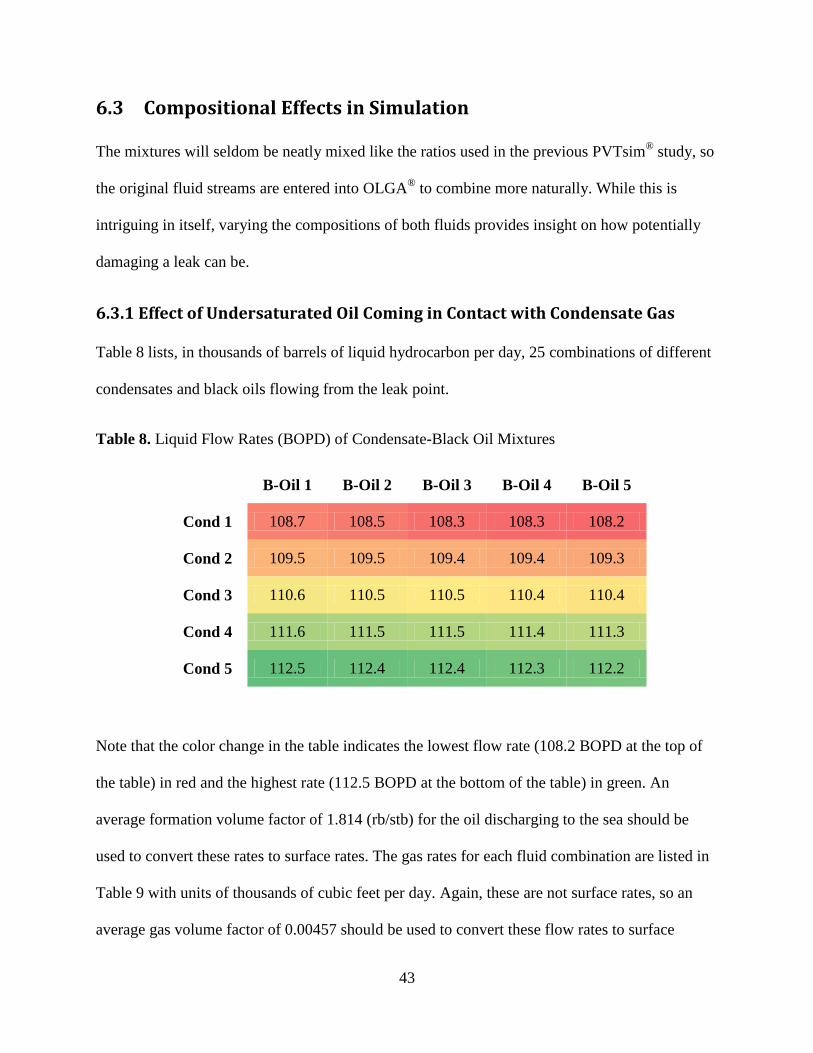
43
6.3 Compositional Effects in Simulation
The mixtures will seldom be neatly mixed like the ratios used in the previous PVTsim® study, so
the original fluid streams are entered into OLGA®
to combine more naturally. While this is
intriguing in itself, varying the compositions of both fluids provides insight on how potentially
damaging a leak can be.
6.3.1 Effect of Undersaturated Oil Coming in Contact with Condensate Gas
Table 8 lists, in thousands of barrels of liquid hydrocarbon per day, 25 combinations of different
condensates and black oils flowing from the leak point.
Table 8. Liquid Flow Rates (BOPD) of Condensate-Black Oil Mixtures
8 Liquid Leak Rates (BOPD) of Condensate-Black Oil Mixtures
B-Oil 1 B-Oil 2 B-Oil 3 B-Oil 4 B-Oil 5
Cond 1 108.7 108.5 108.3 108.3 108.2
Cond 2 109.5 109.5 109.4 109.4 109.3
Cond 3 110.6 110.5 110.5 110.4 110.4
Cond 4 111.6 111.5 111.5 111.4 111.3
Cond 5 112.5 112.4 112.4 112.3 112.2
Note that the color change in the table indicates the lowest flow rate (108.2 BOPD at the top of
the table) in red and the highest rate (112.5 BOPD at the bottom of the table) in green. An
average formation volume factor of 1.814 (rb/stb) for the oil discharging to the sea should be
used to convert these rates to surface rates. The gas rates for each fluid combination are listed in
Table 9 with units of thousands of cubic feet per day. Again, these are not surface rates, so an
average gas volume factor of 0.00457 should be used to convert these flow rates to surface

44
conditions. It is not advisable to simply divide by Bg here because the gas will partially dissolve
in sea water, thereby reducing the quantity of gas actually seen at the surface. However, plume
modeling from offshore spills is not within the scope of this study. For example, the solubility of
methane in pure water at 2,250 psia is approximately 2x10⁻³
mole fraction (Rojey, 1997). One
last point of interest is the general trend seen in the table, which contradicts intuition somewhat.
The lightest black oil in combination with the heaviest condensate yields the most liquid and the
heaviest black oil with the lightest condensate yields the least amount. Steady increments in
liquid flow are to be expected from the gradual increase of the heptanes plus fraction in the
condensate; however, the amount of liquid at the leak decreases slightly with each increase to the
black oil’s heavy fraction.
Table 9. Gas Leak Rates (Mcf/D) of Condensate-Black Oil Mixtures
9 Gas Leak Rates (Mcf/D) of Condensate-Black Oil Mixtures
B-Oil 1 B-Oil 2 B-Oil 3 B-Oil 4 B-Oil 5
Cond 1 1,021.7 1,015.5 1,011.0 1,005.4 1,002.1
Cond 2 1,003.9 999.3 993.6 988.2 984.4
Cond 3 986.5 980.4 975.3 970.3 965.9
Cond 4 967.6 962.1 956.8 951.8 947.4
Cond 5 947.5 941.7 936.4 931.5 927.5
Now a table of GLR values can be generated and used for discharge computations. The question
that remains though concerns the manner in which GLR changes from each wellhead to the
mixing point. If a link can be established between these locations, then a correlation could be
built to better predict leak rates if only bottomhole compositions are known.

45
20 Gas-Liquid Ratio Sampling Points within the OLGA
® Model
Figure 20. In order to assess the changes in GLR within the system, three sampling points are
chosen. The first two places in which the compositions will be measured are the gas tieback and
oil tieback, marked by red dots. The final sampling location is downstream of the T-joint at the
leak itself.
Table 10. Gas-Liquid Ratios (ft3/bbl) from the Gas Tieback Only
10 Gas-Liquid Ratios (ft3/bbl) from the Gas Tieback Only
B-Oil 1 B-Oil 2 B-Oil 3 B-Oil 4 B-Oil 5
Cond 1 10.460 10.527 10.597 10.652 10.721
Cond 2 10.185 10.263 10.322 10.376 10.445
Cond 3 9.925 9.981 10.050 10.097 10.157
Cond 4 9.659 9.727 9.782 9.833 9.889
Cond 5 9.399 9.456 9.509 9.567 9.619
As expected, the heavier the condensate contributing to the flow, the lower the combined GLR
becomes at the leak. The mixtures containing heavier black oils have higher GLR’s compared to
those mixtures with the lighter black oil. This can be explained by considering how the modeled
reservoir fluids were created. All components heavier than hexane were uniformly increased by
5%, 10%, 15% and 20% over the original composition. Even though this reduces the volatile
components in the black oil and allows it to dissolve more gas, the increased density of the

46
mixture actually impedes liquid flow from the black oil well. Liquid flow from the black oil well
reduces by 3.6% between B-Oil 1 and B-Oil 5, regardless of the condensate with which it mixes.
Table 11. Percent Change in Gas-Liquid Ratios from Wellheads to Leak Point.
11 Percent Change in Gas-Liquid Ratios from Wellheads to Leak Point.
B-Oil 1 B-Oil 2 B-Oil 3 B-Oil 4 B-Oil 5
Cond 1 -11.26% -12.53% -13.57% -14.71% -15.79%
Cond 2 -11.14% -12.48% -13.68% -14.83% -15.98%
Cond 3 -11.29% -12.54% -13.84% -14.90% -16.05%
Cond 4 -11.39% -12.76% -13.96% -15.09% -16.20%
Cond 5 -11.59% -12.89% -14.12% -15.31% -16.40%
The black oil, with a bubble point of about 1,480 psia, is undersaturated up to the mixing point;
therefore, the GLR in the oil tieback is equal to Rsoi in all 25 permutations. Table 11 shows the
amount the GLR changes from the wellheads to the leak. As the color coding indicates, the GLR
does not correlate as strongly with the condensate well as it does with the black oil well.
6.3.2 Estimating GOR with Heptanes Plus Fraction
Using the same bank of 25 fluids, an effort was made to extrapolate fluid properties from only
knowing the C7+ fraction of each fluid. McCain (1994) discusses the control heavy components
have over reservoir fluid behavior and generalizes fluid characterization upon C7+ concentration
and a few other parameters. Figure 21 is reproduced from McCain (1994) to show the
dependence of initial GOR on heptanes-plus and how it may be used to make correlations.

47
21 Initial GOR Veresus Heavy Components Fraction
Figure 21. The initial gas-oil ratio ties together rather nicely with the amount of C7+ present in
the reservoir fluids surveyed by McCain (1994). This chart includes fluids ranging from black
oils to wet gases.
Although Figure 21 was reproduced from McCain’s (1994) data set, the curve-fitting was
calculated and may not match exactly as an explicit equation is not provided in the paper.
Converting the GLR’s from Table 10 allows the fluids studied herein to be plotted on this same
chart. Despite lacking as many data points, a trend line for the data can still be constructed.
Figure 22 appears promising, but the exponent determined for the trend line is too different for
the correlation to McCain’s data to be used for fluid mixtures involving anything lighter than
condensate gases. The percent error below a heptanes-plus concentration of 10%, where the
study takes place, should be considered the lower limit when using this relationship.
y = 77008x-1.301 R² = 0.9861
0
20,000
40,000
60,000
80,000
100,000
0 10 20 30 40 50
Init
ial G
OR
, scf
/STB
Heptanes Plus in Reservoir Fluid, mole %
Initial GOR Versus Heavy Components Fraction

48
22 Fitting Simulation Data to the Overall Fluid Trend
Figure 22. The 25 data points extracted from the OLGA® simulations are used to fit a power law
trend line like the one used in McCain (1994).
If the range of fluids considered is reduced to those containing between approximately 5% and
20% heptanes-plus, then a clearer picture of how well this correlation works is visible. Figure 23
zooms further in on this section of the curve and compares the results of different methods
available for predicting the gas-oil ratio from the heavies fraction. Since the trend line for the
McCain data is grounded in several points of actual data, it is plotted again and used as a metric
for determining how well the other methods might predict actual fluids. In addition, a ±10%
error window for this data is also shown.
y = 268403x-1.761
y = 77008x-1.301
0
2,000
4,000
6,000
8,000
0 10 20 30 40 50
GLR
, [sc
f/ST
B]
C7+ Concentration, [%]
Fitting Simulation Data to the Overall Fluid Trend
Surface GOR from OLGA Simulations
McCain's Correlation

49
23 Comparing Various Methods for Predicting GOR
Figure 23. A suite of options exist for estimating the gas-oil ratio when limited data is available;
most of these require the composition to be fully specified.
First, a number of trials were run in the OLGA®
simulator with various pressures for each
reservoir to furnish data points for curve-fitting. The gas condensate reservoir pressure was held
constant at 7,000 psia initially while the black oil reservoir pressure was set to 6,000 psia and
increased by 1,000 psia increments for each new trial. Compositions were sampled within the
OLGA® simulation results at two points: just before mixing and at the leak point. The methods
calculated by PVTsim® and OLGA
® require the full composition to generate mixtures. However,
only the heptanes-plus fractions found just before mixing are needed for calculating GORs with
the proposed correlation. Regardless of method, once a mixture’s heavies-fraction can be
0
1000
2000
3000
4000
5000
5 10 15 20
Gas
-Oil
Rat
io, [
scf/
STB
]
Concentration of Heptanes Plus, [%]
Comparing Various Methods for Predicting GOR
PVTsim Calculation OLGA Simulation Series4
Allocation Method Power (McCain Dataset) Power (McCain ±10%)

50
determined, McCain’s correlation can be applied to estimate the resulting fluid GOR. Assuming
the physics modeled in OLGA® are correct, then the C7+ fraction listed at the leak point after
simulation should provide input for McCain’s correlation to get a close approximation of gas-
liquid ratios expected at the seafloor (after adjusting for pressures and temperatures). Figure 23
does not show the GOR calculated with McCain’s correlation with this heptanes-plus fraction as
it would simply fall along the trend line shown. However, the GORs provided by the simulator
are plotted as “OLGA®
Simulation” in green triangles to compare with this line and fall within
less than 4% save for one outlier that underestimates GOR by about 12%.
PVTsim® can do something different with the leak point compositions, though, by flashing them
to surface conditions. These results are labeled “PVTsim® Calculation” and are marked by red
squares in Figure 23 and agree with the McCain correlation to within less than ten percent.
Another of PVTsim®’s tools is the allocation method previously described at the end of Chapter
3. This software routine consistently predicts GORs to be 20% to 25% higher than the McCain
correlation. Implementing the allocation method is perhaps the quickest if flow rates and
composition are known at the pressure and temperature of interest. However, one can estimate
with even less information by using only the flow rates and heptanes-plus fraction. McCain’s
(1994) discussion of the influence of heavy components to reservoir fluid behavior partly led to
the development of this faster calculation method.
The proposed correlation, denoted by purple circles in Figure 23, requires the volumetric flow
rates, and their respective densities, from each fluid stream as well as the heptanes-plus fraction
for each. Normalizing each stream’s mass flow contribution by the sum of all mass flows
aggregating at the mixing point provides a weighting mechanism (see Equation 6.1) for the C7+
fractions at the mix point.

51
Mixture
C
s
C
s
s p
s
p
s
p
p
s
p
s
p
ZZQ
Q
77
2,1
2,1 2,1
2,1
(6.1)
The subscripts s and p represent well stream source and phase, respectively, while 7CZ denotes
the molar fraction of heptanes-plus. However, it is noted that this simple weighting function
increases in error as the difference in flow from one source dominates the other. In order to
account for this, the increasing difference between actual C7+ concentration and the predicted C7+
concentration is plotted against the difference in pressure between the contributing reservoirs.
Applying this fix removes the gradual drift from accuracy, which tends to increase in a parabolic
manner as displayed in Figure 24.
24 Drift in Heptanes-Plus Prediction While Developing Correlation
Figure 24. The increasing error in predicting the fraction of heavies within the combined fluids
versus the relative strengths of the reservoirs is plotted. Here, the pressure of the condensate
reservoir is subtracted from the black oil reservoir; the convention of subtracting the lighter-fluid
reservoir pressure from the heavier-fluid reservoir must be maintained to use this correlation.
y = -7E-08x2 + 0.0006x + 4.6894 R² = 0.9887
0
1
2
3
4
5
6
7
-2000 -1000 0 1000 2000 3000 4000 5000 6000 Pre
dic
ted
Min
us
Act
ual
C7
+ Fr
acti
on
, [m
ole
s]
Difference between Reservoir Pressures, psia
Differences in Heptanes-Plus Prediction

52
This correction need only be subtracted from the mixture’s heptanes-plus fraction calculated in
Equation 6.1 earlier.
AdjustedMixture
C
Mixture
C ZPPZ ,428
777.4106107
(6.1)
The ΔP here specifically refers to the pressure of the reservoir containing the denser fluid minus
the reservoir pressure contributing the lighter fluid to the mixture. The procedure can be
visualized in the flow diagram provided in Figure 25.
25 Correlation Procedure Diagram
Figure 25. The process of combining disparate fluids from two different paths is procedurally
short, but collection of pertinent data and actual calculation is better left to computer software.
Regarding the process in Figure 25 above, the starting point is always the same and focuses on
simple knowledge of fluid properties and flow within the system. Simulators or nodal analysis
can provide the relative rates of each contributing well or fluid source before the mixing point.
Fluid samples can provide the heptanes-plus fraction of each stream, which will be weighted by
the flow rates just determined. At this point, the method can vary some as the drift of predicted-
to actual C7+ fraction will vary. Note that the abscissa in Figure 24 used to create the trend for
Determine liquid and gas
flow rates from first well just
before the mixing point
Determine liquid and gas
flow rates from second well
just before the mixing point
Find mass rates
using densities of
each phase present
Use mass rates to
create weighted
average of C7+ fraction
Determine heptanes-
plus fraction from the
first well stream
Determine heptanes-
plus fraction from the
second well stream
Correct C7+ fraction
using difference in
reservoir pressures
Use McCain
correlation to
approximate GOR
Predict pressure
loss through leak

53
this drift is the heavier fluid’s reservoir pressure minus the lighter fluid’s reservoir pressure. This
presents a problem for those situations containing more than one fluid source, but this may be
handled with a hierarchical mixing scheme presented in Figure 26. Similar fluids are treated first
with the proposed method to create pseudo-fluids, which are then combined with the disparate
fluids (or pseudo-fluids) in turn.
26 Hierarchical Mixing
Figure 26. A hierarchy of mixing allows use of the proposed method with a complex mixture
containing more than two constituent fluid sources.
The final prediction of C7+ mole fraction can then be used in the McCain relationship to find the
mixture’s GOR. This last piece of information is what the leak pressure drop hinges upon and
provides greater accuracy in fluid discharge. One last thing to note is that the proposed
correlation appears to predict a GOR lower than what is expected by the McCain correlation
whereas the allocation method in PVTsim® consistently predicts too large a value (see Figure
23). The proposed correlation is preferred because it falls more closely within the spread of
McCain’s actual data points; however, an average between the new correlation and the allocation
method may be used if either seems to err too much and both of these methods are very easy to
obtain.
Condensate 1
Condensate 2
Volatile Oil 1
Black Oil 1
Black Oil 2
Pseudofluid 1
Pseudofluid 2
Pseudofluid 3
Final Mixture

54
Chapter 7: Conclusions
Conclusions
The depths to which companies now drill require a tremendous amount of engineering,
technology and capital. Producing from limited slots on platforms creates the need to operate
satellite fields, which in turn opens up the risks associated with hydrocarbons releasing directly
to the seafloor. Each aggregation in the network of flow lines is an area of mixing and possible
leak point carrying fluids with seldom known properties. Knowing these fluid properties allows
for relative rate calculations and the magnitude of the ensuing accident.
7.1 Performance Relationships Dependencies
Results of several simulations concerning aggregation of reservoir fluids, with varying physical
and chemical properties, in a subsea field development have been presented. Chapter two began
by setting up a generic scenario and discussed the most important parameters responsible for
pressure losses. These variables were found within the tubing performance relationship primarily
and, when changed even modest amounts, changed the flow rates much more than the properties
of the reservoir. The one exception to this conclusion is the GOR of the fluid as the advent of
multiphase flow greatly increases pressure drops in the flow path.
7.2 Position and Shape of Leak
Different locations of leak points and the hole geometries through which fluids escape were
discussed. For the worst case of unobstructed flow from a pipe, data from Ashford (1974) was
used to validate different methods of calculating choke flow. The initial attempt of modeling the
leak with OLGA® did not produce accurate results, nor did it compare well with the alternatives
discussed. A built-in correlation, utilizing a default value of 0.84 for the discharge coefficient,

55
allowed OLGA® to vastly improve the accuracy of its flow rate calculations. The coefficient can
be changed to handle arbitrary leaks as one value will never suffice in a real-world situation.
However, using Equation 4.1 provides an even better fit to the data furnished by Ashford (1974).
In other words, finding a means to bring OLGA®’s built-in correlation to the level of Gilbert’s
will allow better estimations of hydrocarbon leaks. Determining a proper discharge coefficient
continues to be the limiting factor regarding this improvement, but may be helped with the aid of
CFD as discussed in the suggestions on future research below.
7.3 A New Correlation When Information is Scarce
The danger and irregularity associated with blowouts causes a good deal of difficulty when
attempting to calculate discharge to the environment. Even when a reservoir has been mapped
out and a well’s profile is fully described, the manner in which merging fluids combine alters
properties and behavior in uncertain ways. Either an expensive simulator or a TPR-IPR analysis
can provide an idea of flow rates contributed by individual well streams. Complete fluid
characterization or quantifying at least the heptanes-plus fraction in each constituent fluid allows
for estimation of the heavies fraction. Ultimately, the GOR of the resulting mixture can be
predicted with the correlation developed herein. This fluid parameter is important in the
discharge equation originally put forth by Gilbert (1954) and improves understanding of pressure
losses experienced at a leak point. This information can then be fed into the iterative solution
process illustrated in Chapter 2.
7.4 Suggestions on Future Work
CFD modeling can greatly aid this study by fine-tuning the smaller elements of the system not
captured by OLGA®. For instance, the wellhead flange connection need not be entirely rendered

56
in such a program (see Figure 27 for a small section of a typical flange and its mating gasket).
Since the equipment is cylindrical, the symmetry can be exploited by only visualizing a quarter
or eighth of the flange connection where a hole has eroded. A complete failure could be modeled
in the same way, except without a gasket to abate flow, and the result multiplied by four or eight
(depending on the modeler’s preference of simplifying the geometry).
27 CFD Model of Well Flange Leak Point
Figure 27. The modeling of a cylindrical well flange is simplified by considering only that
portion which is leaking or by making a representative gap which circumscribe the connection.
Another consideration to make when expanding this study is the amount of wells contributing to
the leak. Only two wells are considered presently, but the addition of a third well would
complicate the mixing even further. However, the difference in fluid composition of the nth
well
is not likely to be as different if it taps into the same reservoir as those nearby. If this assumption

57
is correct then the number of converging fluids can be reduced from the number of contributing
wells to the number of disparate reservoirs contributing.

58
Bibliography
Ajienka, J.A., Enaibe, O.E. and Owolabi, O.O. 1994. Multiphase Flow Metering: An Evaluation
of Discharge Coefficients. Journal of Canadian Petroleum Technology 33 (8): 57-62.
Al-Meshari, Ali A. and McCain, William. 2007. Validation of Splitting the Hydrocarbon Plus
Fraction: First Step in Tuning Equation of State. Paper SPE 104631 presented at the 15th
SPE Middle East Oil & Gas Show and Conference, Kingdom of Bahrain. March 11-14.
Anderson, D. 2012. Flow Assurance with OLGA®
7. SPT Group Industry Course. May 9-11.
Ansari, A.M., Sylvester, N.D., Sarica, C., Shoham, O., and Brill, J.P. 1994. A Comprehensive
Mechanistic Model for Upward Two-Phase Flow in Wellbores. SPE Production and
Facilities 9 (2): 143-151.
Ashford, F.E. 1974. An Evaluation of Critical Multiphase Flow Performance through Wellhead
Chokes. Journal of Petroleum Technology 26 (8): 843-850.
Baxendell, P.B. and Thomas, R. 1961. The Calculation of Pressure Gradients in High-Rate
Flowing Wells. Paper presented at Joint AIChE-SPE Symposium, Tulsa, Oklahoma.
September 25-28, 1960.
Bendiksen, K.H., Malnes, D., Moe, R. and Nuland, S. 1991. The Dynamic Two-Fluid Model
OLGA®: Theory and Application. SPE Production Engineering 6 (2): 171-180.
Bird, R.B., Stewart, W.E., and Lightfoot, E.N. 2007. Transport Phenomena, 2nd
edition. Pages
12-84.
Brown, K.E. and Lee, J.F. 1985. Nodal Systems Analysis of Oil and Gas Wells. Journal of
Petroleum Technology 37 (10): 1751-1763.
Courant, R., Friedrichs, K. and Lewy, H. 1967. On the Partial Difference Equations of
Mathematical Physics. IBM Journal of Research and Development 11 (2): 215-234.
Craft, B.C., Hawkins, M.F., Jr. and Terry, R.E.: Applied Petroleum Reservoir Engineering. New
Jersey: Hall, Inc.

59
Duns, H. and Ros, N.C.J. 1963. Vertical Flow of Gas and Liquid Mixtures in Wells. Paper
presented at the 6th
Annual World Petroleum Congress, Frankfurt am Main, Germany,
June 19-26.
El-Banbi, A.H., Fattah, K.A. and Sayyouh, M.H. 2006. New Modified Black-Oil Correlations for
Gas Condensate and Volatile Oil Fluids. Paper SPE 102240 presented at the SPE Annual
Technical Conference and Exhibition, San Antonio, Texas, USA. September 24-27.
Engineering Toolbox. 2013. Emissivity Coefficients of Some Common Materials. Downloaded
February 19.
Forrest, J., Marcucci, E. and Scott, P. 2005. Geothermal Gradients and Subsurface Temperatures
in the Northern Gulf of Mexico. Search and Discovery Article #30048 in GCAGS
Transactions 55: 233-248.
Gilbert, W.E. 1954. Flowing and Gas-Lift Well Performance. Drilling and Production Practice
(API) 126-43.
Gulf of Mexico. 2013. Scale not determined; James Stiernberg; using “Google Maps”.
https://maps.google.com/maps?q=gulf+of+mexico&ll=27.771051,-
90.615234&spn=7.345348,9.876709&hnear=Gulf+of+Mexico&t=h&z=7 (accessed
March 11, 2013).
Hagedorn, A.R. and Brown, K.E. 1963. The Effect of Liquid Viscosity in Two-Phase Vertical
Flow. Paper SPE 733 presented at the SPE Fall Meeting in New Orleans, 6-9 October.
Hasan, A.R. and Kabir, C.S. 2002. Fluid Flow and Heat Transfer in Wellbores. Richardson, TX:
Society of Petroleum Engineers, Inc., pages 1-62.
Hein, M.A. 1987. Nodal Analysis as Applied to Pipelines and Risers. Paper presented at Pipeline
Simulation Interest Group in Tulsa, Oklahoma, 22-23 October.
Iwere, F.O., Heim, R.N., and Cherian, B.V. 2012. Numerical Simulation of Enhanced Oil
Recovery in the Middle Bakken and Upper Three Forks Tight Oil Reservoirs of the
Williston Basin. Paper SPE 154937 presented at the Americas Unconventional Resources
Conference in Pittsburgh, PA, June 5-7.
Job, G. and Herrmann, F. 2006. Chemical Potential—A Quantity in Search of Recognition.
European Journal of Physics 27 (2): 353-371.
Langlinais, J. 2013. Two Phase Flow. File last modified March 2013. Microsoft Excel file.

60
Lietz, W. Tempelaar. 1949. The Performance of the Ten Section Oil Field. Journal of Petroleum
Technology 1 (9): 251-258.
Mach, J., Proano, E., and Brown, K.E. 1979. A Nodal Approach for Applying Systems Analysis
to the Flowing and Artificial Lift Oil or Gas Well. OnePetro, http://www.onepetro.org/.
Accessed 26 February 2012.
Massoud, M. 2005. Engineering Thermofluids: Thermodynamics, Fluid Mechanics and Heat
Transfer. Berlin: Springer.
McCain, William D. 1990. The Properties of Petroleum Fluids, Second Edition. Tulsa,
Oklahoma: PennWell Books.
McCain, William D. 1994. Heavy Components Control Reservoir Fluid Behavior. Journal of
Petroleum Technology 46 (9): 746-750.
Millheim, K., Williams, T.E., Yemington, C.R. 2011. Evaluation of Well Testing Systems for
Three Deepwater Gulf of Mexico (GOM) Reservoir Types. Paper SPE 145682 prepared
for the SPE Annual Technical Conference and Exhibition in Denver, CO, Oct. 30-Nov. 2
Moore, T.V. and Wilde, H.D. 1931. Experimental Measurements of Slippage in Flow through
Vertical Pipe. Trans. Am. Inst. Mining Met. Engrs. (Petroleum Development and
Technology) 114 (99): 296-319.
Muskat, M. 1949. Physical Principles of Oil Production. New York: McGraw-Hill.
Navier, L.M.H. 1827. Mémoires de l'Académie Royale des Sciences 6: 389-440.
Nichol, J.R. and Kariyawasam, S.N. 2000. Risk Assessment of Temporarily Abandoned or Shut-
in Wells. Report for the Department of Interior, Mineral Management Service.
Nodine, M.C., Wright, S.G., Gilbert, R.B. and Ward, E.G. 2006. Mudflows and Mudslides
During Hurricane Ivan. Paper presented at the Offshore Technology Conference in
Houston, Texas, May 1-4.
OLGA®. 2012. Computer software manual by SPT Group. Version 7.2, released September 27.
Payne, L. and Sandeen, J. 2013. Emerging Plays Boost Economic Attractiveness of Deepwater
Gulf of Mexico. The Way Ahead 9 (1): 11-13.

61
Pedersen, K.S. and Milter, J. 2004. Phase Equilibrium Between Gas Condensate and Brine at
HT/HP Conditions. Paper SPE 90309 presented at the SPE Annual Technical Conference
and Exhibition in Houston, Texas, September 26-29.
Pedersen, K.S. 2005. PVT Software Applied with Multiphase Meters for Oil & Gas Allocation.
Presented at the Flow 2005: Modeling, Metering and Allocation conference in Aberdeen,
Scotland, March 14-15.
Peneloux, A., Rauzy, E., Freze, R. 1982. A Consistent Correction for Redlich-Kwong-Soave
Volumes. Phase Equilibria 8 (1): 7-23.
Peng, D. and Robinson, D.B. 1976. A New Two-Constant Equation of State. Ind. Eng. Chem.
Fundamentals 15 (1): 59-64.
Poettmann, F.H. and Carpenter, P.G. 1952. The Multiphase Flow of Gas, Oil, and Water
Through Vertical Flow Strings with Application to the Design of Gas-Lift Installations.
Presented at the spring meeting of the Mid-Continent District, Division of Production,
Wichita, Kansas, March.
PVTsim®. 2012. Computer software manual by Calsep. Version 20.2.0, released April 9.
Rahman, M.M., Biswas, R. and Mahfuz, W.I. 2009. Effects of Beta Ratio and Reynold’s Number
on Coefficient of Discharge of Orifice Meter. Journal of Agricultural and Rural
Development 7 (1&2): 151-156.
Redlich, O. and Kwong, J.N.S. 1949. On the Thermodynamics of Solutions. V—An Equation of
State. Fugacities of Gaseous Solutions. Chem. Reviews 44: 233-244.
Riazi, M. R. and Mansoori, G.A. 1992. An Accurate Equation of State for Hydrocarbon Systems.
Paper SPE 25397 available from SPE, Richardson, Texas.
Rojey, A. 1997. Natural Gas: Production, Processing, Transport. Paris, France: Technip, pages
205-207.
Ros, N.C.J. 1961. An Analysis of Critical Simultaneous Gas/Liquid Flow through a Restriction
and Its Application to Flow Metering. Applied Science Research 9: 843-850.
Soave, G. 1972. Equilibrium Constants from a Modified Redlich-Kwong Equation of State.
Chem. Eng. Sci., 27 (6): 1197-1203.
Stokes, G.G. 1845. Proceedings of the Cambridge Philosophical Society 8: 287-319.

62
Tannehill, J.C., Anderson, D.A. and Pletcher, R.H. 1997. Computational Fluid Mechanics and
Heat Transfer Second Edition. Washington, D.C.: Taylor & Francis, pages 45-60.
Trefethen, L.N. 1996. Finite Difference and Spectral Methods for Ordinary and Partial
Differential Equations. Unpublished text available at
http://people.maths.ox.ac.uk/trefethen/pdetext.html. Downloaded 29 October 2012.
van der Waals, J.D. 1873. Over de Continuiteit van den Gas-en Vloeistoftoestand. Dissertation,
Leiden University, Leiden, Netherlands.
Walsh, M.P. and Lake, L.W. 2003. A Generalized Approach to Primary Hydrocarbon Recovery.
Oxford, UK: Elsevier, pages 209-210.
Weisstein, Eric W. "Courant-Friedrichs-Lewy Condition." From MathWorld--A Wolfram Web
Resource. http://mathworld.wolfram.com/Courant-Friedrichs-LewyCondition.html
White, Frank M. 2006. Viscous Fluid Flow (3rd
Edition). New York: McGraw-Hill.

63
Appendix
A. Fluid Bank
Fluids in this study came from different sources; Al-Meshari and McCain (2007) provide the
initial condensate and black oil fluids denoted by the superscript-daggers in the following tables.
Table 12. Condensate Fluids Used in Studies and Some of Their Properties
12 Condensate Fluids Used in Studies and Some of Their Properties
Component or Property Cond 1† Cond 2 Cond 3 Cond 4 Cond 5
N2 0.29 0.2891 0.2882 0.2872 0.2863
CO2 0.2 0.1994 0.1987 0.1981 0.1975
C1 84.66 84.3900 84.1216 83.8550 83.5900
C2 4.04 4.0271 4.0143 4.0016 3.9889
C3 2.23 2.2229 2.2158 2.2088 2.2018
C4 0.68 0.6778 0.6757 0.6735 0.6714
C5 0.99 0.9868 0.9837 0.9806 0.9775
C6 0.51 0.5084 0.5068 0.5052 0.5036
C7 1.12 1.1722 1.2242 1.2758 1.3270
C8 0.51 0.5338 0.5574 0.5809 0.6043
C9 0.38 0.3977 0.4153 0.4328 0.4502
C10 0.3 0.3140 0.3279 0.3417 0.3555
C11 0.28 0.2931 0.3060 0.3189 0.3318
C12 0.22 0.2303 0.2405 0.2506 0.2607
C13 0.2 0.2093 0.2186 0.2278 0.2370
C14 0.15 0.1570 0.1640 0.1709 0.1777
C15 0.12 0.1256 0.1312 0.1367 0.1422
C16 0.12 0.1256 0.1312 0.1367 0.1422
C17 0.1 0.1047 0.1093 0.1139 0.1185
C18 0.07 0.0733 0.0765 0.0797 0.0829
C19 0.06 0.0628 0.0656 0.0683 0.0711
C20 0.05 0.0523 0.0547 0.0570 0.0592
C21 0.04 0.0419 0.0437 0.0456 0.0474
C22 0.03 0.0314 0.0328 0.0342 0.0355
C23 0.03 0.0314 0.0328 0.0342 0.0355
C24 1.5 1.5700 1.6395 1.7086 1.7773
C25 0.95 0.9943 1.0384 1.0821 1.1256
Pseudocomponent C26-C30 0.09 0.0942 0.0984 0.1025 0.1066
Pseudocomponent C31-C36 0.08 0.0837 0.0874 0.0911 0.0948
Critical Pressure (psia) 4645.2 4748.3 4826.8 4890.4 4941.2
Critical Temperature (°F) 100.7 117.5 132.1 146.1 159.5

64
The compositional tracking module in OLGA®
requires an input called a “feedfile” which limits
the amount of components used to thirty, thereby increasing the granularity of simulation results;
this is mitigated by choosing components similar to each other in any given pseudocomponent.
For example, one pseudocomponent definition groups normal and iso-butane. Thus, the
maximum is used with no pseudocomponent representing more than six individual components).
Table 13. Black Oils Used in Studies and Some of Their Properties
13 Black Oils Used in Studies and Some of Their Properties
Component or Property B-Oil 1† B-Oil 2 B-Oil 3 B-Oil 4 B-Oil 5
N2 0.7960 0.7828 0.7700 0.7576 0.7456
CO2 1.1940 1.1742 1.1550 1.1364 1.1184
H2S 0.4980 0.4897 0.4817 0.4740 0.4665
C1 44.0300 43.2987 42.5913 41.9067 41.2437
C2 5.4730 5.3821 5.2942 5.2091 5.1267
C3 5.2740 5.1864 5.1017 5.0197 4.9402
C4 2.0900 2.0553 2.0217 1.9892 1.9577
C5 3.383 3.3268 3.2725 3.2199 3.1689
C6 3.4830 3.4252 3.3692 3.3150 3.2626
C7 2.8860 2.9800 3.0709 3.1588 3.2440
C8 2.1890 2.2603 2.3292 2.3960 2.4606
C9 1.9200 1.9825 2.0430 2.1015 2.1582
C10 1.6920 1.7471 1.8004 1.8520 1.9019
C11 1.6120 1.6645 1.7153 1.7644 1.8120
C12 1.4330 1.4797 1.5248 1.5685 1.6108
C13 1.3330 1.3764 1.4184 1.4590 1.4984
C14 1.1440 1.1812 1.2173 1.2522 1.2859
C15 0.9550 0.9861 1.0162 1.0453 1.0735
C16 0.9550 0.9861 1.0162 1.0453 1.0735
C17 0.9050 0.9345 0.9630 0.9906 1.0173
C18 0.7160 0.7393 0.7619 0.7837 0.8048
C19 0.6470 0.6681 0.6884 0.7082 0.7273
C20 0.5970 0.6164 0.6352 0.6534 0.6711
C21 0.5470 0.5648 0.5820 0.5987 0.6149
C22 0.5070 0.5235 0.5395 0.5549 0.5699
C23 0.4780 0.4936 0.5086 0.5232 0.5373
C24 3.3830 3.4932 3.5997 3.7028 3.8027
C25 2.587 2.6712 2.7527 2.8316 2.9079
Pseudocomponent C26-C30 1.91 1.9722 2.0323 2.0906 2.1470
Pseudocomponent C31-C36 5.383 5.5583 5.7278 5.8919 6.0508
Critical Pressure (psia) 1480.8 1434.9 1392.4 1353 1316.4
Critical Temperature (°F) 829.8 834.7 839.2 843.3 847.2

65
B. Heat-Transfer Coefficient Calculations
The overall heat-transfer coefficient equation is reproduced here from Chapter 4’s section
discussing the OGLA model.
cem
rr
to
c
rr
to
ann
rr
to
rcci
to
t
rr
to
titi
to
to k
r
k
r
k
r
hhr
r
k
r
hr
r
U
co
cem
ci
co
to
ci
ti
to lnlnln
)(
ln1
(B.1)
The greatest difficulty in determining this number is the temperature-dependent nature of the
heat-transfer coefficients associated with convection. A number of heat-transfer coefficients
must first be found before incorporating all of them together; for example, the first term deals
with conductive heat transfer from the reservoir fluid to the outside surface of the production
tubing.
14.03
18.0
31
8.0 023.0PrRe023.0
w
HC
HC
HCp
HCti
HC
ti
HCti
k
cvd
d
k
d
kh
(B.2)
The produced fluid’s thermal conductivity, kHC, and viscosity, μHC, are required for the Reynolds
number (Re) and the Prandtl number (Pr); these dimensionless numbers are expanded in
Equation B.2 for convenience. The former is a ratio of viscous and inertial forces while the latter,
Prandtl number, is a ratio of momentum diffusivity to thermal diffusivity (White, 2006). An
initial OLGA® simulation is required to obtain an idea of what the superficial fluid velocity is at
the bottom of the well; it is about 36.4 ft/s in the black oil well. The other items required for
these equations, such as dimensions and emissivity, are given in Table 8.

66
Table 14. Well Profile and Material Properties Used in Thermal Calculations
14 Well Profile and Material Properties Used in Thermal Calculations
Parameter Lower Portion Upper Portion
dti (in) = 4.5 5.5
dto (in) = 5 6
dci (in) = 7 10.75
dco (in) = 7.5 11.25
dcem (in) = 8.5 12.25
εsteel, polished†
= 0.075 0.075
koil (Btu/hr-ft-°F) = 0.131 0.132
cp,oil (Btu/lbmol-°F) = 56.63 52.95
ρoil (lbs/ft3) = 53.04 53.04
ρann (lbs/ft3) = 59.14 63.1
μoil (lb/ft-hr) = 1.78 1.773
μann (lb/ft-hr) = 0.8696 3.67
kann (Btu/hr-ft-°F) = 0.406 0.37
ktbg,csg (Btu/hr-ft-°F) = 11.54 11.54
kcem (Btu/hr-ft-°F) = 4.021 4.021
βoil (1/°F) = 0.314 0.314
MWoil (lb/lbmol) = 101.22 101.22
† Measured at 300 Kelvin according to The Engineering Toolbox (2013).
Plugging the proper terms in yields the Reynolds number, the Prandtl number and the first
conductivity value (which has units of Btu/hr-ft2-°F).
168,464,1
)3600/78.1(
375.0*4.36*04.53Re
oil
oilvd
(B.3)
6.7
22.101
1*
131.0
78.1*63.56Pr
,
oiloil
oiloilp
MWk
c
(B.4)
85.494,18696.0
78.16.7168,464,1
375.0
131.0023.0
14.0
31
8.0
tih (B.5)

67
The next heat-transfer coefficients that require some involved manipulation relate to radiation
and convection in the annular space between tubing and casing. The Grashof number (Gr) must
be introduced to proceed with the calculation of the convection term.
16.308696.0
180179)314.0*14.59*2.32(
12
5.2
12
5.3)(
2
2
3
2
23
a
tociatoci
TTgrrGr
(B.6)
The gravity constant, g, uses length units consistent with the density and the fluid expansion
term, β, has units of reciprocal Fahrenheit. Convective heat transfer within the completion brine
between tubing and casing can now be determined.
345.1
208.0
292.0ln
12*2
7
347.0)6.7()6.7*16.30(*049.0
ln
PrPr049.0 074.031
074.031
to
cici
annc
rr
r
kGrh
(B.7)
This number is considerably smaller than the conductive heat-transfer coefficient as expected,
because the tight spacing between tubing and casing walls precludes well-developed convection
cells. Smaller than this though is the coefficient for radiative heat-transfer.
0586.0
1075.0
1
5.2
5.3
075.0
1
)639640)(639640(*9713.1
111
))(( 22**2*2*
e
r
r
TTTTh
cito
ci
ci
tocitocir
(B.8)
The asterisks are reminders for using Rankine instead of Fahrenheit and ε is the emissivity (the
ability to transmit energy in the form of radiation) of the bounding solid surface; it is specific to
the material and measured relative to a black body’s ability to emit radiation, therefore it is
unitless (Massoud, 2005). The Stefan-Boltzmann constant has a value of 1.713x10⁻⁹
for units of

68
reciprocal ft2-hr-°R (Hasan and Kabir, 2002). Combining these values allows for the overall
heat-transfer coefficient to be computed.
406.0
4.1ln*208.0
)0586.0345.1(*292.0
208.0
54.11
11.1ln*208.0
495,1*1875.0
208.01
toU
Btu
Ffthr
2
6913.0021.4
13.1ln*208.0
54.11
071.1ln*208.0
(B.9)
Therefore, the overall coefficient is 1.4465 Btu/hr-ft2-°F at the bottom of the well; this is a
reasonable number since there is little difference in temperature near the source of the fluid. The
coefficient increases with elevation and is largest at the mud line.

69
Vita
James Thomas Stiernberg was born in Galveston, Texas, in 1986. Shortly thereafter, he moved to
Bellaire, Texas for most of elementary school and graduated from Bellaire High School in 2004.
He followed his two brothers, Charles and William, to the Cockrell School of Engineering at the
University of Texas at Austin. He graduated with a Bachelor of Science in Geosystems
Engineering and Hydrogeology in the spring of 2009. He promptly went to work for Halliburton
as a surface data logging field engineer on deepwater drilling rigs in the Gulf of Mexico. In his
final summer before graduating from Louisiana State University, he gained engineering
experience during his internship with Chevron in Bakersfield, California; the company made a
return offer, which he accepted. He enjoys rock climbing, running, swimming, electronics and art
in his spare time.