Embed Size (px)
Citation preview

��������������� ��
���������������������������������
����������������������������
���� !�"� ##�
� � � � � � � � � � � � � � � � � �
�����������������

��������������� ��
����������������������������������
������������������������������
���� !�"� ##�
� ���������������� ������������������������������� � ��������������������������������������������������������������������� ����� � ���������������������������������������������������� ������ ������!�������"������������������������������������������������������#� $������
% ����� &'�����( ������������������
� � � � � � � � � � � � � � � � � �
�����������������

� ������������ ��������
������� ���������������
���������������� !��
"�� �#
$���� ������� $�����%&������
���������������� !��
"�� �#
'� ��&�� ()�����))�
*����� &���+,,---.�%/.��
��0 ()�����))����
'� �0 )���))�%/�
��������������
����������������������������������������������������������������������������������������������
��������������������������������������������������������������������������
�������������� ����
���������������������

������������ ��������������������������� �
��������
��������
�� ����������������� �
�� ������������ �
�� ��������������������� �� �������!������ "
�� #������� �$
� %�&��������������� ���� '���� ������������������������&���������������� ���� #���� �� �����!������ ���� #�������������!������� ��� (����������������)���&���� ������������������������������ �*�� �� ���&���&��&������ �*�* +��������&��&������ ��
�� '���������� �"
,��������� ��
#������������ ���� ��
%���&����'�������-��.����.�� �&�&��������� ��

������������ ���������������������������
Abstract
This paper examines the issue of the impact of aggregation in theempirical analysis of euro area labour markets. A Phillips Curve describingthe adjustment of unit labour costs is estimated at the national and aggregatelevel for the 5 largest euro area countries. Potential sources of aggregationbias are investigated – such as differences in parameter coefficients and alack of correlation in the independent variables across countries – as well asthe potentially offsetting statistical averaging effect. Finally the out-of-sample forecasting performance of both approaches is evaluated. The resultspoint to some limited advantages of analysing wage developments at thenational rather than at the area-wide level. The paper concludes that if majoradvantages in undertaking national analysis do exist, they are likely to arisefrom the ability to develop country-specific structures for the PhillipsCurves and not from aggregation biases that emerge when a commonstructure is used.
JEL Classification: C52, C53, E24, J30 .
Key words: Euro area; Phillips curve; wage growth.
������������ ��������������������������� �
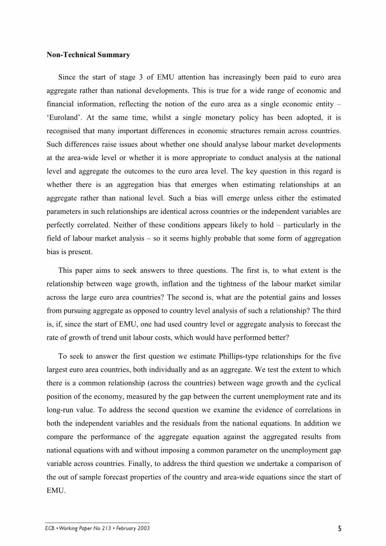
Non-Technical Summary
Since the start of stage 3 of EMU attention has increasingly been paid to euro area
aggregate rather than national developments. This is true for a wide range of economic and
financial information, reflecting the notion of the euro area as a single economic entity –
‘Euroland’. At the same time, whilst a single monetary policy has been adopted, it is
recognised that many important differences in economic structures remain across countries.
Such differences raise issues about whether one should analyse labour market developments
at the area-wide level or whether it is more appropriate to conduct analysis at the national
level and aggregate the outcomes to the euro area level. The key question in this regard is
whether there is an aggregation bias that emerges when estimating relationships at an
aggregate rather than national level. Such a bias will emerge unless either the estimated
parameters in such relationships are identical across countries or the independent variables are
perfectly correlated. Neither of these conditions appears likely to hold – particularly in the
field of labour market analysis – so it seems highly probable that some form of aggregation
bias is present.
This paper aims to seek answers to three questions. The first is, to what extent is the
relationship between wage growth, inflation and the tightness of the labour market similar
across the large euro area countries? The second is, what are the potential gains and losses
from pursuing aggregate as opposed to country level analysis of such a relationship? The third
is, if, since the start of EMU, one had used country level or aggregate analysis to forecast the
rate of growth of trend unit labour costs, which would have performed better?
To seek to answer the first question we estimate Phillips-type relationships for the five
largest euro area countries, both individually and as an aggregate. We test the extent to which
there is a common relationship (across the countries) between wage growth and the cyclical
position of the economy, measured by the gap between the current unemployment rate and its
long-run value. To address the second question we examine the evidence of correlations in
both the independent variables and the residuals from the national equations. In addition we
compare the performance of the aggregate equation against the aggregated results from
national equations with and without imposing a common parameter on the unemployment gap
variable across countries. Finally, to address the third question we undertake a comparison of
the out of sample forecast properties of the country and area-wide equations since the start of
EMU.

������������ ���������������������������*
In answer to the first question, our analysis suggests that freely estimated Phillips curves
do generate different estimates of the impact of unemployment gap on wage formation.
However, when estimated jointly in a panel system, these differences do not prove to be
statistically significant and it is possible to impose a common unemployment gap effect.
Nevertheless, many national idiosyncrasies remain in the equations.
In answer to the second question, the value of area-wide analysis is enhanced if there is a
similarity in parameters across the national equations, a high positive correlation between the
independent variables and a negative correlation between the residuals from the national
equations. As already indicated, the evidence on the common parameters was mixed, with it
being possible to impose a restriction on the unemployment gap parameter. All the other unit
labour cost and price variables, as well as the constant, showed marked differences across
countries. It is also noteworthy that for most of the independent variables we found evidence
of positive and statistically significant cross-country correlations. Overall there did not appear
to be evidence of strong correlation – either positive or negative – in the residuals from the
national equations. In addition, to further shed light on this second question we estimated an
aggregate unit labour cost equation and compared the results with the aggregation of results
from the national equations. Although the statistical properties of the area-wide equation were
quite good overall, its standard error was slightly higher than the aggregated standard errors
from the national equations, both estimated independently and as a system.
In relation to the third question, we found that if the Phillips curves developed in this
paper had been used, then this variable would have been slightly better predicted if the
national approach had been adopted and the results aggregated. However, the gains from the
diasaggregate approach tended to disappear as the forecast horizon lengthened. One caveat
here is that, if a constant rather than the time-varying NAIRU computed by the OECD is
assumed, the relative forecast performance of the area-wide approach deteriorates further.

������������ ��������������������������� �
1. Introduction2
Since the start of stage 3 of EMU attention has increasingly been paid to euro area
aggregate rather than national developments. This is true for a wide range of economic and
financial information, reflecting the notion of the euro area as a single economic entity –
‘Euroland’. At the same time, whilst a single monetary policy has been adopted, it is
recognised that many important differences in economic structures remain across countries.
Nowhere is this more evident than in labour markets. Structural features relating to labour
market institutions, the legislative framework and social security systems differ to a large
degree across the euro area countries. Such differences raise issues about whether one should
analyse labour market developments at the area-wide level or whether it is more appropriate
to conduct analysis at the national level and aggregate the outcomes to the euro area level.
There is a growing literature on aggregation issues which is summarised in Dedola et al
(2001). Much of the recent work has focussed on the aggregation of money demand
relationships (Fagan and Henry (1998), Dedola et al (2001)) but some analysis has also been
undertaken with respect to labour markets (Turner and Seghezza (1999) and OECD (2000)).
The question that is often addressed by researchers is whether there is an aggregation bias that
emerges when estimating relationships at an aggregate rather than national level. As discussed
in Fagan and Henry (1998) an aggregation bias will emerge unless either the estimated
parameters in such relationships are identical across countries or the independent variables are
perfectly correlated. Neither of these conditions appears likely to hold – particularly in the
field of labour market analysis – so it seems highly probable that some form of aggregation
bias is present.
It is then necessary to investigate how large such a bias is and whether there are any
potentially offsetting factors that make it more useful to conduct an area-wide analysis rather
than estimating national relationships. As Fagan and Henry (1998) discuss, the magnitude of
the bias depends positively on the extent to which the parameter coefficients are different and
inversely on the degree of correlation in the movement of the independent variables at the
national level. A potential offsetting factor is what is known as the statistical averaging effect.
This emerges because, typically, the variance of the weighted sum of the country equation
2 This paper was presented at the 3rd ECB Labour Market Workshop, held in Frankfurt on the 10th-11th ofDecember 2001. We thank, without implicating, Olivier de Bandt, Michael Burda, Gabriel Fagan, DennisSnower, an anonymous referee and other participants to the workshop.

������������ ���������������������������/
residuals is lower than the variance of the residuals in any one country. In other words some
residuals will tend to offset each other leading to lower residuals at the aggregate rather than
national level. The extent to which this happens clearly depends on the degree of correlation
in the residuals across countries. Another way of looking at this, as argued by OECD (2000),
is that the national equations may be mis-specified in that they wrongly exclude important
area wide variables. For example, in the context of money demand, national equations would
be affected by foreign variables if there was currency substitution within European portfolios.
This may lead to negative cross-country correlations in the residuals from national money
demand equations.
The issue of the validity of aggregation therefore becomes an empirical question on the
extent to which parameters differ across countries and on the comparison of the correlations
in both the independent variables and the residuals. In the context of money demand, Fagan
and Henry (1998) estimate a long-run money demand function on 14 EU countries and at the
aggregate level. Despite the fact that there are marked differences in the parameter estimates
between the national equations, they find a superior performance of the aggregate equation
with a lower standard error and stronger evidence for cointegration than the national
equations. The statistical averaging effects are found to lower the standard error at the
aggregate level, as there is a small tendency towards a negative correlation in the residuals
from national equations. However, a point forcefully made by Dedola et al (2001) is that it is
not necessarily appropriate to compare the performance of an aggregate equation against the
performance of a typical national equation. Rather comparison should be made between the
performance of the aggregate equation and the performance of the aggregated results from the
national equations. This way the statistical averaging effect of residuals falls out of the
comparison and no longer serves to favour the aggregate approach. Nevertheless, in the paper
by Fagan and Henry (1998), the aggregate money demand equation still outperforms the
aggregation of national equations.
This paper aims to make a practical contribution to this debate in the context of labour
market analysis by seeking answers to three questions. The first is, to what extent is the
relationship between wage growth, inflation and the tightness of the labour market similar
across the large euro area countries? The second is, what are the potential gains and losses
from pursuing aggregate as opposed to country level analysis of such a relationship? The third
is, if, since the start of EMU, one had used country level or aggregate analysis to forecast the
rate of growth of trend unit labour costs, which would have performed better?

������������ ��������������������������� "
To seek to answer the first question we estimate Phillips-type relationships for the five
largest euro area countries, both individually and as an aggregate. We test the extent to which
there is a common relationship across the five countries between wage growth and the
cyclical position of the economy, measured by the gap between the current unemployment
rate and its long-run value. To address the second question we examine the evidence of
correlations in both the independent variables and the residuals from the national equations. In
addition we compare the performance of the aggregate equation against the aggregated results
from national equations with and without imposing a common parameter on the
unemployment gap variable across countries. Finally, to address the third question we
undertake a comparison of the out of sample forecast properties of the country and area-wide
equations since the start of EMU.
The paper is structured as follows. In the next section we discuss the specification adopted
to model the dynamics of wage growth. Next we report estimates of the aggregate and
national equations. In the latter cases these are estimated separately and as a system to test
whether the restriction of a common parameter on the unemployment gap is accepted. We
also provide evidence on the correlation structure in the independent variables and the single
equation residuals. The residuals of the various approaches are compared. The paper then
gives details of the out of sample forecast properties of the approaches before concluding.
2. An Overview of the Wage Growth Equation
We examine the potential importance of aggregation biases in labour markets using a
simple wage-price Phillips curve (following Gordon (1997)). The equation describes a
disequilibrium adjustment process in the labour market: the change in nominal wages adjusted
for trend productivity growth provides a measure of trend unit labour costs. This is postulated
to depend on price inflation and labour market tightness. Price inflation is measured by the
first difference in (the log of) consumption deflator (current and lagged values). In the
absence of a specific measure of expected inflation, this lag structure is assumed to capture
both price inertia and the formation of inflationary expectations. Labour market tightness is
measured by the unemployment gap, that is, the difference between the actual rate of
unemployment and the NAIRU, where the latter is computed as a filtered version of observed
unemployment. The equation also contains shocks to import prices as an additional factor
which might influence wage growth other than the stance of the labour market.

������������ ����������������������������$
The specification chosen includes among the regressors lagged values of the dependent
variable, lagged values of the change in (the log of) consumer prices and import prices (in
second differences) and current values of the unemployment gap.
t
p
jjitj
h
jjitj
k
jjitjtt zpmgpdulccbgapaulc ∑ +∆∆∑ +∆∑ +∆++=∆
=−
=−
=−
001lnlnlnln (1)
where ulc is the ratio of nominal wages to trend labour productivity, p is the consumers’
expenditure deflator, pm is the import deflator, gap is the difference between the
unemployment rate (ILO measure) and the time-varying NAIRU and z is an error term.
As is standard practice in Phillips curve-based analysis, a long-run nominal homogeneity
restriction is imposed. This assumption guarantees the existence of an equilibrium in the
labour market and implies that inflation depends only on nominal factors in the long run, that
is: 14
0
4
1
=+∑∑== j
jj
j dc .3
The choice of analysing a reduced-form relationship such as the Phillips Curve described
above is partly motivated by the idea that an area-wide approach might be more justified for
an empirical analysis of the euro area labour market based on this type of relationship rather
than, say, on a structural model. It is in fact sometimes argued that the Phillips Curve
approach and, relatedly, the concept of NAIRU, is more relevant for large closed economies
(such as the US) than for small open ones, where domestic factors play a lesser role in
determining inflation when compared to foreign variables such as the exchange rate and
competitiveness. Indeed, as indicated in Fabiani and Mestre (2000, 2001), area-wide estimates
of the NAIRU show significant inflation forecasting ability and are able to produce sensible
measures of the output gap at the euro area level.
3. The Data
Data for the five largest euro area countries are seasonally adjusted quarterly time series
collected from various sources, namely the ESA95 database published by Eurostat, the
Quarterly National Account (QNA), the Quarterly Labour Force Statistics and the Main
3 For a detailed explanation of the implications of the assumption of long-run homogeneity, see Fabiani andMestre (2000).

������������ ��������������������������� ��
Economic Indicators (MEI) databases published by the OECD and the BIS database. The time
range covered by the series differs across countries. In order to achieve the highest possible
degree of comparability we selected a common sample period, starting in 1982q1 and ending
in 2000q4.
Data on GDP, final consumption of households, imports of goods and services (all at
constant and current prices), the number of employees and total compensation of employees
at current prices were available from the ESA95 database since 1978q1 for France, 1970q1
for Italy, 1980q1 for Spain and 1991q1 for Germany.
For Germany, data prior to 1991 were reconstructed by the authors using time series for
West Germany from different sources: namely the QNA database for GDP at current and
constant prices, private final consumption expenditure at current and constant prices, imports
of goods and services at current and constant prices and the BIS database for compensation of
employees and the number of employees for the whole economy. In order to be coherent with
the seasonally adjusted ESA95 data available since 1991, as a first step the data prior to 1991
from the QNA database were adjusted for seasonal effects by the authors.4
For the Netherlands, ESA95 data on GDP and imports at constant and current prices are
available from 1977q1, while time series on private final consumption started only in 1995.
For the latter, the BIS private consumption deflator series, seasonally adjusted and starting in
1977q1, was used.
For the unemployment rate, Eurostat standardised unemployment rate series available on
the OECD MEI database were used for all countries, with the exception of Italy, for which the
series for unemployment in the Centre-North provided by Banca d’Italia was adopted5. Trend
unemployment (or the NAIRU) was derived by filtering the unemployment rate series for
each country using the standard Hodrick-Prescott methodology. Finally, data on total
employment for all countries were taken from the OECD Quarterly Labour Force Statistics
database. Trend unit labour costs time series were constructed as follows. First an estimate of
4 Using the package available in the FAME software.5 As a first attempt, we tried to model the Phillips curve by computing the unemployment gap on the basis
of the national unemployment rate, as in the other countries. This variable, however, performed verypoorly, in line with the claim, often made in the literature on the subject, that the strong regionalsegmentation of the Italian labour market implies that unemployment in the Northern regions is the mainfactor affecting the bargaining process and hence the determination of wages in Italy (see also Fabiani atal (1997), Turner and Seghezza (1999)).

������������ �����������������������������
whole economy productivity was derived as the ratio of real GDP to total employment. This
series was smoothed with a Hodrick-Prescott filter to obtain a measure of trend productivity.
Trend unit labour costs were then calculated as the ratio of wages (compensation per
employee) to trend productivity. The consumption deflator was computed as the ratio of
nominal to real private consumption expenditure, with the exception of the Netherlands, as
mentioned above. The import deflator was obtained as the ratio of nominal to real imports of
goods and services, for all countries.
In order to compare the results at the single country level with those obtained at the area-
wide level, the national data for trend unit labour costs, the consumption deflator, the import
deflator, the unemployment rate described above were aggregated into area-wide variables.6
For this purpose, we adopted the so-called index method: national nominal and price variables
were transformed into logarithms and then aggregated using fixed weights, namely GDP at
PPP exchange rates for 1995. These weights were also used to compute the area-wide
unemployment rate. As stressed by Fagan and Henry (1998) this approach has the advantage
of facilitating the comparison of results from area-wide and national equations.
4. Empirical evidence
4.1. Cross-correlations in the independent variables
As discussed in the introduction, the degree of correlation in the national independent
variables is an important indicator of the extent to which aggregation biases may be relevant.
To recap, the higher the degree of correlation in the movement of the independent variables at
the national level the smaller the expected magnitude of the aggregation bias. As shown in
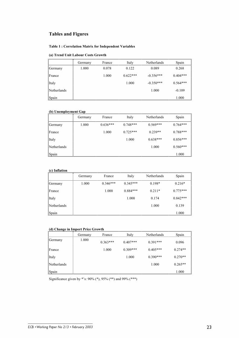
Table 1, which gives details of the correlations in the independent variables across countries,
we generally find a positive and statistically significant correlation coefficients. In the case of
the change in the log of trend unit labour costs the correlation coefficient is around 0.4 to 0.6
for France-Italy, France-Spain and Italy-Spain and highly statistically significant. The
correlation coefficients for each country with respect to Germany are also positive, but lower
in magnitude and not statistically significant. However, in the case of the Netherlands the
6 For the main methods of constructing consistent aggregate data from disaggregate ones, see Fagan andHenry (1998).

������������ ��������������������������� ��
correlation coefficients with the other countries are generally negative. The overall average of
the correlation coefficients was 0.14. As for the unemployment gap, there is a significant and
generally large positive correlation for all pairs of countries. The overall average correlation
coefficient was 0.65. For the inflation variable, that is, the first difference of the log of the
consumers’ expenditure deflator, all correlation coefficients are positive, and most are
statistically significant, with an overall average of 0.41. Finally, in all cases there is a positive
correlation in the change in the log of import price growth across the 5 countries, with the
overall average being 0.32. In all but one case these correlation coefficients are statistically
significant.7
4.2. The Aggregate Equation
We estimated an area-wide Phillips curve described in equation 1 using data obtained by
aggregating the time series of the five countries. Prior to the estimation, we tested for
stationarity of the unit labour cost growth and inflation time series by means of standard
Augmented Dickey Fuller tests. As the last two rows of Table 2 show, it is possible to reject
the null hypothesis that both series have a unit root when an order of augmentation of the test
of at least two is selected.
After having ascertained that the series were stationary, a search for the preferred
specification of the Phillips curve was undertaken. Both Akaike and Schwartz selection
criteria suggested the introduction of only one lagged value of the dependent variable among
the regressors. As for the independent variables, the preferred specification was one that
included three lags of price inflation, the current change in import price inflation. For the
variable measuring the stance of the labour market, we followed Gordon (1996) in including
the current value of the unemployment gap and, as a result of our specification search, we
choose not to enter first differences of the unemployment rate as an additional regressor
capturing hysteresis effects. The final specification adopted was:
titj
jitjittt zqDqDqDpmepdulccbgapaulc ++++∆∆∑ +∆+∆++=∆=
−− 198291284lnlnlnln3
11 (2)
7 It should be noted that these correlations relate to the variables as used in the equation. In their raw formthe correlation coefficients are generally much higher – in fact in the case of wages and the consumers’expenditure deflator they range from 0.96 to 0.99.

������������ ����������������������������
Where D84q2 and D91q2 are time dummy variables accounting for large outliers in German
data. The first relates to a major period of industrial unrest whilst the second relates to
reunification. The dummy variable labelled as D98q1 accounts instead for a break in the
series of compensation of employees for Italy, due to the introduction of a new tax scheme
(IRAP). In order to achieve nominal dynamic homogeneity in the long run, we imposed the
restriction c+d1+d2+d3=1.
The OLS estimates of the aggregate Phillips curve for the period 1982:1 2000:48 are
reported in the last column of Table 3. The unemployment gap term is correctly signed and
significant with a coefficient of –0.0016.
The statistical properties of the model are quite satisfactory. The long-run homogeneity
restriction is not rejected by the data. The goodness of fit is high, considering that the
equation is specified in first differences and that the estimation period covers a long period of
time. The LM test for serial correlation shows that the chosen specification captures quite
well the dynamic properties of the endogenous variable, while the RESET test supports the
validity of the linear specification. The estimated equation exhibits no signs of
heteroscedasticity. In order to verify whether the relationship linking nominal wage growth to
inflation and the unemployment gap has undergone significant modifications during the
estimation period we followed two different strategies. First, we estimated the equation up to
1998:1 and used the obtained coefficients to predict the wage growth pattern over the
following two years. The Chow test for the adequacy of such predictions does not seem to
signal the existence of a structural break in the relationship. Second, given that the timing of
structural breaks cannot in general be established a priori, we performed a Hansen test aimed
at detecting instability of a general form (which is approximately an LM test of the null of
constant parameters against the alternative that they follow a martingale). The test was carried
out on the overall equation and on some relevant parameters. As the last column of Table 4
shows, none of the parameters show signs of instability and the statistic for the entire equation
is well below the 5% critical value.
8 This was the longest period for which data were available for all countries.

������������ ��������������������������� ��
4.3. The National Equations
After having investigated the stationarity properties of the national series of trend unit
labour cost growth and inflation (see Table 2), equation (1) was estimated for each single
country. The results of the OLS regressions are reported in the first five columns of Table 3.
Excluding the case of France, the unemployment gap always has the expected negative
coefficient, ranging from –0.0014 in Italy to –0.0037 in Germany. For France and Italy the
coefficient is not significantly different from zero. For the other countries, the statistical
significance of the unemployment gap coefficient is quite high, as it has a t-statistic in the
range of 2.6-2.9.
As each national model is specified exactly as the one chosen for the aggregate equation
and its performance varies quite widely across countries. The estimated equation performs
quite poorly in the case of France, showing signs of residual auto-correlation and
heteroscedasticity, but reasonably well for the remaining countries. Hansen tests (reported in
the first five columns of Table 4) point to a certain degree of instability of the overall equation
for France and Germany, although the result for latter is driven by the necessity to exclude the
dummy variables from the specification for carrying out the test. In the case of the
Netherlands the test finds evidence of instability for the unemployment gap coefficient.
Conversely, Chow tests for stability of the regression coefficients for 1999:1-2000:4 and
predictive failure tests based on estimates for the period up to 1998:4 both reject the
hypothesis of a structural break at the start of Stage 3 of EMU.
Table 5 gives details of the cross correlation matrix of the national OLS residuals. In
general, there is somewhat mixed evidence on the co-movement of these residuals, but in
almost all cases the results are not statistically significant. The correlation coefficients for the
residuals of the German equations and each of the other countries are negative except in the
case of Italy. A negative pattern emerges also for the correlation coefficients for the residuals
of Netherlands-Spain and France-Spain. It appears that there is some sign of a small mutual
positive correlation in the other residuals, although the coefficients are nearly all below 0.3.
The lack of a strong positive correlation in the residuals means that the aggregate equation
should benefit from the statistical averaging effect described in the introduction, leading to a
lower standard error than is present in the typical national equation.

������������ ����������������������������*
4.4. System estimation: imposing restrictions across countries
The national Phillips Curves were then estimated together as a panel system with fixed
effects and (following Turner and Seghezza, 1999) tested for the imposition of a common
unemployment gap term across countries.9 As this assumption was not rejected by the data, it
was imposed and the results reported in Table 6. Overall, the pattern of results is similar to the
individual OLS regressions. The main notable improvement is an increase in the significance
of the unemployment gap term which, at –0.002 is slightly larger in magnitude than in the
aggregate equation..
It is noteworthy that this finding of a common parameter on the unemployment gap for
these countries finds some support from other studies. Morgan and Mourougane (2001), who
estimate a panel system including a structural wage and labour demand equation for the same
five countries and in addition the UK, find that it is possible to impose a common
unemployment parameter. Turner and Seghezza (1999), who estimate a Phillips Curve with
an output gap variable using a SURE system, also find that it is possible to impose a common
coefficient for the gap variable for a wide group of OECD countries.
Although the restriction required for the long-run nominal dynamic homogeneity in the
wage-price system was imposed in all countries, we did not investigate the extent to which it
would be possible to impose a common price dynamics, i.e. common coefficients on trend
unit labour cost, consumer and import prices. It is clear from the tables that although it may
be possible to group individual parameters in some countries, it is highly unlikely to be
possible to group them all given the range of outcomes reported in the tables (as for of them
the estimated coefficients are positive and significant in one country and negative and
significant in another).
4.5. In-Sample Properties
Despite the generally satisfactory nature of the area-wide equation, as Dedola et al (2001)
point out, it is necessary to compare its residuals with those obtained by aggregating the
9 Another approach would have been to implement a Seemingly Unrelated Regression Estimation (SURE).However for such an approach to have been worthwhile there would needed to have been a clear sign thatthere was a correlation in the residuals from the national equations.

������������ ��������������������������� ��
residuals from the national equations. For this purpose, we have aggregated the national
residuals derived from the estimation exercises (both single OLS and system estimates)
described in the first part of this section, using the same weights adopted to construct the area-
wide variables. Figure 1 compares the aggregated residuals from the single OLS and the
restricted system estimation with the residuals from the area-wide equation. Table 7 also gives
details of the respective standard errors. Both the table and the graph clearly show that the
volatility of the area-wide residuals is slightly higher than that of the aggregated national
ones. In particular, the OLS single country estimation seems to generate residuals that, once
aggregated, provide the lowest standard error. According to the test of Grunfeld and Griliches
(1960), this provides grounds for selecting the disaggregate model over the aggregate one.
However, it should be noted that the differences in the standard errors are not particularly
large – ranging from 0.29% for the aggregated national equations to 0.30% for the system and
the aggregate approach. The difference of 0.01% compares with an average quarterly change
in aggregate unit labour costs of 0.7% over the estimation period.
4.6. Forecast Properties
The last part of this empirical section focuses on the performance of our Phillips Curves in
forecasting aggregate trend unit labour costs. More precisely, we investigate the out-of-
sample forecast properties of the area-wide equation as compared with the aggregation of the
out-of-sample forecasts based on the national equations. It should be emphasised that the
results presented here should be seen as simple tests of the performance of the equations
analysed thus far in this paper and are not the outcome of a careful fine-tuning of equations
providing optimal forecasts of area-wide wage growth.
The approach to out of sample forecasting that we adopted here is that of Staiger et al
(1997), based on recursive least squares. This approach provides a consistent way to evaluate
real-time forecasting performance, since at each point in time the forecast is truly out of
sample. We examined what forecasts would have been made during each quarter from the
start of 1999 to the end of 2000 based on quarterly data for the period from 1982q1 up to the
quarter when the forecast was made, by estimating our equations on actual data over the same

������������ ����������������������������/
time period.10 For example, for 1999q1 we estimated the equation up to this quarter, we
derived a forecast for the next four quarters and we saved the 1, 2 3, and 4 steps ahead
forecast errors. The process was then repeated for 1999q2, using data up to that date and a
new set of 1, 2, 3 and 4 step ahead errors was saved. After having repeated this exercise
recursively until the quarter before the last (i.e. 2000q3) we computed the Mean Absolute
Error (MAE), the Root Mean Square Error (RMSE) and the Theil’s U statistics (U) for 1, 2, 3
and 4 steps ahead (Table 8).11
Table 8 is divided into two panels. The first panel is based on forecast errors generated by
aggregating the five national wage growth forecasts; the second panel refers instead to the
forecasting performance of the area-wide equation. In both cases the equations used to
compute each forecast have exactly the same specification as the ones adopted in the OLS
exercise described above.
Both the RMSE and the Theil’s U statistic are lower in the top panel for the first two rows,
corresponding to the forecasts for 1 and 2 steps ahead. However, the better forecasting
performance of the national equations is not maintained for the 3 and 4 steps ahead forecasts.
Hence, the results presented in the table indicate that if one had used the Phillips curve to
forecast aggregate trend unit labour cost growth since the start of 1999, then such a variable
would have been better predicted if one had relied on national equations and then aggregated
the results rather than adopting an area-wide specification. However, if one had wished to
predict the rate of growth of trend unit labour costs more than six months ahead, then there
would have been no benefit in using national equations. The gain from using the national
equations, in terms of lower RMSEs, was 0.02 for both the 1 and 2 period ahead forecasts.
This compares with an average quarter-on-quarter growth rate in the variable about 0.3% over
the forecast horizon.
In specifying the Phillips Curve, we have so far computed the NAIRU in each country and
at the area-wide level as a smoothed version of observed unemployment. In order to check the
robustness of the results, we also considered an alternative framework, based on the
assumption that the NAIRU is constant over the whole time horizon. In other words, we
10 When running the n-steps ahead forecasts we used autoregressive processes (with four lags and aconstant) to generate subsequent observations for the regressors (inflation, unemployment, the NAIRUand the change in the import deflator).

������������ ��������������������������� �"
modelled trend unit labour cost growth as depending on the actual unemployment rate instead
of the unemployment gap.12 The pattern of results obtained under these alternative hypotheses
framework was very similar to that described above, as are the standard errors for both the
aggregated and aggregate results. However, under the hypothesis of constant NAIRU the
forecasting ability of the area-wide equation was markedly worse than when using a time-
varying NAIRU. Although the performance of the national equations also worsened when
using a constant NAIRU, the deterioration in the forecast performance of the area-wide
equation was much more marked.13
5. Conclusions
At the start of this paper we set out to find information to help answer three questions. The
first was the extent to which the relationship between wages and productivity growth,
inflation and the tightness of the labour market is similar in the large euro area countries. Our
analysis suggests that freely estimated Phillips curves do generate different estimates of the
impact of the rate of unemployment on wage formation. However, when estimated jointly in a
panel system, these differences do not prove to be statistically significant and it is possible to
impose a common unemployment gap effect. Nevertheless, many national idiosyncrasies
remain, which, within the reduced form equation considered in this paper, are captured by the
constant and by the dynamic pattern of consumer and import prices.
The second question related to the potential gains and losses from pursuing aggregate as
opposed to country-level analysis of such relationships. As discussed in the early part of the
paper, the value of area-wide analysis is enhanced if there is a similarity in parameters across
the national equations, a high positive correlation between the independent variables and a
negative correlation between the residuals from the national equations. As already indicated,
the evidence on the common parameters was mixed, with it being possible to impose a
restriction on the unemployment gap parameter. All the other unit labour cost and price
variables, as well as the constant, showed marked differences across countries. It is also
11 The Theil’s U statistic is a unit-free measure computed as the ratio of the root mean square error to theroot mean square error of the ‘naïve’ forecast of no change in the dependent variable. A value of zeroimplies no forecast error.
12 The constant NAIRU then forms a part of the constant.13 Full results using the constant NAIRU are available upon request from the authors.

������������ ����������������������������$
noteworthy that for most of the independent variables we found evidence of positive and
statistically significant cross-country correlations. Overall there did not appear to be evidence
of strong correlation – either positive or negative – in the residuals from the national
equations. In addition, to further shed light on this second question we estimated an aggregate
unit labour cost equation and compared the results with the aggregation of results from the
national equations. Although the statistical properties of the area-wide equation were quite
good overall, its standard error was slightly higher than the aggregated standard errors from
the national equations, both estimated independently and as a system.
The third question was, if, since the start of EMU, you had used country-based or area-
wide analysis to forecast aggregate unit labour cost growth, which would have performed
better? We found that if the Phillips curves developed in this paper had been used, then this
variable would have been slightly better predicted if the national approach had been adopted
and the results aggregated. However, the gains from the diasaggregate approach tended to
disappear as the forecast horizon lengthened. One caveat here is that, if a constant rather than
the time-varying NAIRU computed by the OECD is assumed, the relative forecast
performance of the area-wide approach deteriorates further.
Overall, our results point to some limited advantages from estimating wage-price Phillips
Curves at the national level rather than conducting the analysis at the area-wide level. Most
notably the standard errors and the 1-period ahead out-of-sample forecasts from the
aggregated national equations are found to be lower than those from the area-wide equation.
However, the differences between the forecast errors disappear at longer horizons (3-4 periods
ahead) are not large. Furthermore, some support for adopting an area-wide approach in
Phillips curves-based analysis stems from the fact that it proved possible to impose a common
coefficient on the unemployment gap across countries and that there is some positive
correlation in the movements of some of the national independent variables.
These results are open to different interpretations. In support of the aggregate approach, it
could be argued that the key finding is the common unemployment coefficient. The other
coefficients – on lagged prices – reflect expectations formation and the properties of the
inflation process which clearly, in the past, differed a lot across countries. Given the move to
monetary union, we may expect a tendency towards a common inflation process and
convergence of expectations formation. In other words, the coefficients on lagged inflation
may become more similar across countries over time. Therefore the relative position of the
aggregate approach may improve over time. Alternatively, it could be argued that the simple

������������ ��������������������������� ��
models used in the paper do not do justice to the more sophisticated, detailed type of analysis
which could be carried out at the national level. Indeed, one of the key advantages of national
as opposed to aggregate analysis may lie in the possibility to take account of country-specific
features in the specification of the Phillips Curves, rather than adopting a common
specification as we do here. Hence the results may provide only a lower bound estimate of the
likely superiority of bottom-up versus top-down approaches to area-wide labour market
analysis. Nevertheless, our results suggest that if major advantages in undertaking national
analysis do exist, they are likely to arise from the ability to develop country-specific
structures for the Phillips Curves and not from aggregation biases that emerge when a
common structure is used.
������������ �����������������������������
References
Dedola, L., E. Gaiotti and L. Silipo (2001), “Money Demand in the Euro Area: DoNational Differences Matter?”, Temi di Discussione, Banca d’Italia No. 405.
Fabiani S., A. Locarno, G. Oneto and P. Sestito (1997), “NAIRU: Incomes Policy andInflation”, OECD Economics Department Working Papers No. 187.
Fabiani S. and R. Mestre (2000), “Alternative estimates of the NAIRU in the euro area:estimates and assessment”, ECB Working Paper No. 17.
Fabiani, S. and R. Mestre (2001), “A system approach for measuring the euro areaNAIRU”, ECB Working Paper No 65.
Fagan, G. and J. Henry (1998), “Long run money demand in the EU: evidence from area-wide aggregates”, Empirical Economics, Vol. 23 pp. 483-506.
Gordon, R. (1997), “The Time-Varying NAIRU and its Implications for EconomicPolicy”, Journal of Economic Perspectives, Winter 1997; 11(1): 11-32
Gruen, D., A. Pagan and C. Thompson (1999), “The Phillips Curve in Australia”, ReserveBank of Australia Research Discussion Paper No 1999-01.
Grunfeld, Y. and Z. Griliches (1960), “Is aggregation necessarily bad?”, The Review ofEconomics and Statistics, Vol.17, pp.1-13.
Hansen, B. E. (1994), “Testing for Parameter Instability in Linear Models”, in N. R.Ericsson and Irons, J. S. (eds.) Testing exogeneity, Oxford, Oxford University Press.
Lucifora, C. and P. Sestito (1993), “Determinazione del salario in Italia: una rassegnadella letteratura empirica”, Istituto di Economia dell’Impresa e del Lavoro, Discussion PaperNo. 5
Morgan, J. and A. Mourougane (2001), “What can changes in structural factors tell usabout unemployment in Europe”, ECB Working Paper No. 81.
OECD (2000), “Could aggregation be misleading?”, in Emu one year on, OECD, Paris.
Staiger, D., J. H. Stock and M. W. Watson (1997), “The NAIRU, Unemployment andMonetary Policy”, Journal of Economic Perspectives, Vol. 11(1), pp. 33-49.
Turner, D. and E. Seghezza (1999), “Testing for a Common OECD Phillips Curve”,OECD Economics Department Working Papers No. 219.
������������ ��������������������������� ��
Tables and Figures
Table 1 : Correlation Matrix for Independent Variables
(a) Trend Unit Labour Costs Growth
Germany France Italy Netherlands Spain
Germany 1.000 0.078 0.122 0.089 0.268
France 1.000 0.622*** -0.356*** 0.404***
Italy 1.000 -0.350*** 0.564***
Netherlands 1.000 -0.109
Spain 1.000
(b) Unemployment Gap
Germany France Italy Netherlands Spain
Germany 1.000 0.636*** 0.748*** 0.569*** 0.764***
France 1.000 0.725*** 0.239** 0.788***
Italy 1.000 0.638*** 0.856***
Netherlands 1.000 0.560***
Spain 1.000
(c) Inflation
Germany France Italy Netherlands Spain
Germany 1.000 0.346*** 0.345*** 0.198* 0.216*
France 1.000 0.884*** 0.211* 0.775***
Italy 1.000 0.174 0.842***
Netherlands 1.000 0.139
Spain 1.000
(d) Change in Import Price Growth
Germany France Italy Netherlands Spain
Germany 1.0000.363*** 0.407*** 0.391*** 0.096
France 1.000 0.309*** 0.405*** 0.274**
Italy 1.000 0.390*** 0.270**
Netherlands 1.000 0.265**
Spain 1.000
Significance given by *’s: 90% (*), 95% (**) and 99% (***)

������������ ����������������������������
Table 2: Stationarity tests
Variable
c c,t c c,t c c,t c c,t c c,t
France DULC -4.36 -5.55 -3.07 -3.48 -2.86 -3.18 -3.41 -4.10 -3.07 -3.68 DPC -3.89 -4.76 -4.04 -4.03 -3.97 -3.67 -4.37 -4.73 -4.68 -4.42
Germany DULC -9.13 -9.34 -5.32 -5.52 -3.98 -4.19 -2.98 -3.18 -2.04 -2.22 DPC -5.23 -5.18 -4.24 -4.21 -2.89 -2.87 -2.16 -2.13 -2.02 -1.98
Italy DULC -4.79 -6.39 -3.78 -5.33 -3.02 -4.03 -2.85 -3.74 -2.73 -3.52 DPC -2.80 -3.90 -2.64 -3.26 -2.85 -2.92 -2.95 -2.88 -2.83 -2.86
Netherlands DULC -3.01 -3.72 -2.29 -2.91 -2.13 -2.77 -2.62 -3.39 -2.41 -3.23 DPC -10.28 -10.36 -5.91 -5.91 -5.14 -5.14 -3.22 -3.23 -2.65 -2.64
Spain DULC -5.50 -6.37 -3.58 -3.98 -3.37 -3.79 -3.24 -3.71 -2.69 -2.92 DPC -3.19 -5.31 -2.33 -3.46 -2.21 -3.22 -2.18 -3.30 -2.12 -2.54
Aggregate DULC -5.63 -7.31 -3.25 -4.28 -2.49 -3.27 -2.29 -2.99 -2.02 -2.50 DPC -3.28 -3.88 -2.91 -3.31 -2.71 -2.61 -2.69 -2.57 -2.77 -2.50
Notes:
For each lag, the two columns report the results of Dickey-Fuller regressions including an intercept (c ) and including an intercept and a time trend (c,t ), respectively
The 95% critical value for the ADF statistics is -2.9 in the regression (c) and -3.5 in the regression (c,t )
ADF(4)ADF ADF(1) ADF(2) ADF(3)
Table 3: OLS estimation for individual countries and 5-country aggregate
Variable France Germany Italy Netherlands Spain Aggregate
Constant -0.0017 (2.98) -0.0013 (1.55) -0.0031 (3.42) -0.0006 (1.32) -0.0012 (1.57) -0.0021 (4.91)GAPt 0.0001 (0.07) -0.0037 (2.79) -0.0014 (0.70) -0.0027 (2.63) -0.0019 (2.88) -0.0016 (2.04)DULCt-1 0.2872 (2.16) -0.1278 (1.50) 0.2085 (1.88) 0.7079 (9.37) 0.2408 (1.91) 0.0696 (0.75)DPCt-1 0.3326 (1.44) 0.3951 (2.37) 0.4203 (1.61) 0.1008 (1.73) 0.6244 (3.00) 0.5010 (2.79)DPCt-2 0.0329 (0.15) 0.1876 (0.93) 0.5068 (1.59) 0.0675 (1.20) -0.1144 (0.57) 0.0723 (0.32)DPCt-3 0.3473 (2.25) 0.5451 (3.29) -0.1356 (0.50) 0.1237 (2.11) 0.2493 (1.38) 0.3570 (2.11)DDPMt 0.0124 (0.44) 0.1324 (2.39) 0.0497 (1.47) 0.0019 (0.10) -0.0568 (1.09) 0.0682 (2.22)d84q2 -0.4107 (5.61) -0.0176 (5.03)d91q2 0.0337 (4.59) 0.0153 (4.38)d98q1 -0.0283 (4.18) -0.0062 (1.82)
R(bar)2
DW
SE
Homogeneity restriction - χ2(1) 5.6465 [0.017] 0.5097 [0.475] 2.1928 [0.139] 5.2967 [0.021] 9.6705 [0.002] 2.5692 [0.109]
A - Serial correlation - χ2(4) 15.8336 [0.003] 4.6366 [0.327] 2.5431 [0.637] 5.6370 [0.228] 7.0066 [0.136] 5.0731 [0.280]
B - Functional form - χ2(1) 2.8795 [0.090] 1.2975 [0.255] 0.3080 [0.579] 0.0496 [0.824] 3.2031 [0.073] 0.4721 [0.492]
C - Normality - χ2(2) 1.2284 [0.541] 0.3772 [0.828] 0.1249 [0.939] 1.3269 [0.515] 0.3238 [0.851] 1.8520 [0.396]
D - Heteroscedasticity - (χ2(1)) 5.3481 [0.021] 0.1826 [0.669] 1.3452 [0.246] 2.3690 [0.124] 0.4509 [0.502] 1.2277 [0.268]
E - Predictive Failure (χ2(8)) 11.4063 [0.180] 7.2976 [0.505] 1.6240 [0.990] 4.9867 [0.759] 3.1129 [0.927] 7.6699 [0.466]
F - Chow test (χ2(6)) 11.2071 [0.082] 4.0573 [0.669] 2.9360 [0.817]
Notes: Brackets show absolute values of t statistics; square brackes show the significance level of the reported tests.A: Lagrange multiplier tests of residual serial correlation; B: Ramset’s RESET test using the square of fitted values; C: based on a test of skewness and kurtosis of residuals; D: based on the regression of squared residuals on squared fitted values; E: test of adequacy of predictions for 1999:1- 2000:4 based on the estimates for the period up to 1998:4 (Chow second test); F: test for stability of the regression coefficients for 1999:1- 2000:4 based on the estimates for the period up to 1998:4 (Chow first test).
0.4864
2.0974
0.0044
2.1314
0.0034
0.5646
1.9021
0.0066
0.6002
1.6625
0.0068
0.6923
1.9138
0.0032
0.3651
2.1465
0.0061
0.5808

������������ ��������������������������� ��
Table 4: Hansen stability tests for individual countries and 5-country aggregate OLS equations
Variable France Germany Italy Netherlands Spain Aggregate
Equation 2.655 3.025 1.034 1.676 1.618 1.783
GAPt 0.384 0.078 0.088 0.679 0.132 0.055DULCt-1 0.274 0.094 0.086 0.081 0.097 0.066DPCt-1 0.074 0.254 0.129 0.477 0.062 0.176DPCt-2 0.039 0.062 0.122 0.486 0.036 0.139DPCt-3 0.074 0.099 0.117 0.280 0.093 0.130DDPMt 0.225 0.199 0.316 0.084 0.113 0.092
NotesThe 5% critical values are 0.470 for individual coefficients and 2.110 for the whole equationThe test for Germany and for the aggregate was run without including the dummy variables.
Table 5: Correlation Matrix for the Residuals from the National OLS Equations
Germany France Italy Netherlands Spain
Germany 1.000 -0.141 0.139 -0.115 -0.202*
France 1.000 0.012 0.309***-0.031
Italy 1.000 0.066 0.101
Netherlands 1.000 -0.126
Spain 1.000
Significance given by *’s: 90% (*), 95% (**) and 99% (***)
Table 6: Restricted Pooled estimation for individual countries
Variable France Germany Italy Netherlands Spain
Constant -0.0017 -(2.22) -0.0013 -(1.90) -0.0032 -(4.09) -0.0005 -(0.74) -0.0012 -(1.71)GAPt -0.0020 -(4.39) -0.0020 -(4.39) -0.0020 -(4.39) -0.0020 -(4.39) -0.0020 -(4.39)DULCt-1 0.3218 (1.90) -0.0866 -(1.31) 0.1995 (2.19) 0.7357 (6.73) 0.2306 (2.09)DPCt-1 0.2384 (0.82) 0.4040 (2.93) 0.4205 (1.91) 0.0926 (0.97) 0.6283 (3.29)DPCt-2 0.0732 (0.27) 0.1613 (0.96) 0.5084 (1.89) 0.0553 (0.61) -0.1117 -(0.61)DPCt-3 0.3666 (1.85) 0.5213 (3.81) -0.1284 -(0.57) 0.1164 (1.21) 0.2528 (1.53)DDPMt 0.0102 (0.28) 0.1310 (2.86) 0.0490 (1.72) 0.0000 (0.00) -0.0587 -(1.24)d84q2 -0.0422 -(7.00)d91q2 0.0362 (6.15)d98q1 -0.0284 -(4.96)
R(bar)2 0.6232SE 0.0056χ2(4) test for the equality of the coefficient of GAPt for all countries = 5.0855 [p-value=0.279]

������������ ����������������������������*
Table 7: Standard error of residuals
National OLS 0.0029Restricted pooled system 0.0030Aggregate OLS 0.0030
Table 8: Out of sample recursive forecasts of aggregate wage growth
mean absolute error root mean squared error Theil U
steps ahead
1 0.0023 0.0031 0.93892 0.0027 0.0031 0.99343 0.0021 0.0026 1.20594 0.002 0.0024 0.7320
steps ahead
1 0.0027 0.0033 0.98542 0.0028 0.0033 1.04783 0.0021 0.0024 1.10794 0.0020 0.0024 0.7097
NotesTheil U is computed as the ratio of the root mean square error to the root mean square error of a "naive" forecast of no change in the dependent variable
aggregate equation
national equations
Figure 1 : Residuals from the Aggregate, National and Panel Equations
-0.01
-0.008
-0.006
-0.004
-0.002
0
0.002
0.004
0.006
0.008
0.01
AGGREGATE
NATIONAL
PANEL

������������ ��������������������������� ��
�������������� ���������������������
�������� ���� ���������������������� ������������������� ���� ������������!��"������#����$%%"""&���&���'&
((� )������ �������������������������������������������$��������� ������������ ������ �������*�����&������+&�,�������-&�.��� � ��+����/00/&
((1 )2�����������������������������$�"�������"������3*����4&�5��� �����5&�-������&�2�6�����&�7� �88�����+����/00/&
((9 )2�������� ����� �������������������� ���������� ����$�� ��"����������������*���5&�:�����������������/00(&
((; )<�������������������������������=�����(>?9����(>>?*����+&�@�����������&�-�8&�+����/00/&
((� )@�������������������"������������������$��������������"��� ��������������*���:&��� ������&�A� � ��+����/00/&
((? )��� ������������������B������C� ���������$����� ����������������� ����������4� ���(>??D(>>?*����=&�2&�7�����+����/00/&
((> )2�������� ����������������������������������*����.&����� �����&�2���+����/00/&
(/0 ),���������� �����������������"���������������������*����E&�@������6����-&�2���+����/00/&
(/( ).�� ����������*����5&���������<&��&�5&������������/00/&
(// ).�"������� ���������������� ������"���������������*�����&�A�6�� ����<&�5 ����������/00/&
(/� )5� ��������������������� ��� ���������������������������� �������������*�����&�7�������5&�A������������/00/&
(/1 )2�������� ������B�����������������������*����=&��&�� ������E&�@������6�������/00/&
(/9 )�������� � ������� � �� �����������������*����E&�2���� ���������/00/&
(/; ):���� ������������������������ ������� �������������� *�����&�2���������&�F��������������/00/&
(/� )��������������������� ����"��������� ����� ��������������*����E&�@������6���-&�2����������/00/&
(/? ):�������������������B������������D������������������� ���*�����&�E�������<&���������������/00/&
������������ ����������������������������/
(/> ).��D���������� ����� ������������������"���������������������C�� ����*���5&� D.�"�������,&�E�����2���/00/&
(�0 )@����8�������B�������������������$�������������� �����������*�����&����"���2���/00/&
(�( )2��������������������@4��$�"������"�����"�����"������"�������������"3*���2&�5&�����������&�<��G���8D� ��8�� ��2���/00/&
(�/ )4�� ������������������ ���� �������������������������$��)��"�-�������*�������� �*����:&�5���� ���&�<��G���8D� ��8�� �����&�7�������2���/00/&
(�� )������������������������������� ��������������������� �=�����"��3*���5&�2�����������2&�<����2���/00/&
(�1 )7������������� ���������������������.���� �����(>>/D(>>>*�����&��������+&�A��� ����2���/00/&
(�9 )7�������� ���B�����B����������������������������������*�����&������������&�7� ����5�� �/00/&
(�; )<��� �������������������D������$�������"�� ������������������� � � *���=&�����������5�� �/00/&
(�� )�C�� ������������������������������!��������������������*����H&�������� ��5�� /00/&
(�? ).�"*� ��"�������������������������������$�"�������2H��� ������3*����&��&�2���� ���5�� �/00/&
(�> ):��������������������������*����2&���8������5�� �/00/&
(10 )�������������������������D������������������� ����*����2&�������2��/00/&
(1( )5������������������ �� ����*�����&��������������,&�E�����������2��/00/&
(1/ )2��� ���������� ������������������ �����������������B��������� �C��������������������������������� ����*�����5&�������=&����D2����8��5&�@���������&�.�����2��/00/&
(1� )5����D����������������� �������"������*�����4&��"�����2��/00/&
(11 )5��� �������������������������� ����$���� ���������������������������B���������������������*�����2&�E� �����E&�@� ���2��/00/&
(19 )7�"������"�� ��"��������������������� ������*�����2&���8��������2&���������2��/00/&
(1; )������������������� ����I�"��!������� ������������3*������&�� ���������&�@�����2��/00/&

������������ ��������������������������� �"
(1� )7���D��D��� ��������������������������������"���������8��������������� ����2&�������2��/00/&
(1? )7����������� ����������� ���� ��*����A&����������2��/00/&
(1> )7���E������� ������������E��D�� ��D����������� *����5&���������5&��� ����2�/00/&
(90 )�C���������������������� ���� ������������������������� ���*����<&�=����+&�A�� ����=&�A� �����+����/00/&
(9( )=D����� ������������*�����&���� ��+����/00/&
(9/ )E���D��������������������� ��� ���������� ���*����=&����D2����8����5&�,����+���/00/&
(9� )����������������������������������� �������$������ �������������������*���5&��� ����+����/00/&
(91 )7�������� ���������� �� ��������������� ��$���"��������������� ��������������������B���������� �B��� ���������������������������"� �3*����2&���8������+����/00/&
(99 )J���������� ��������������:���$������������������� �������������������������������������������*����+&��&�+����������&�<������8D� ��8�� ��+����/00/&
(9; )4�������������������������� ��� ����� ���������������������� �*����+&�+&����8�����&�@�������+� ��/00/&
(9� )����������������������������������$�� ���������������������������������*���-&�=&�.������H&�������� ����4&�5&�E���� � ��+� ��/00/&
(9? )F�������������������7����� ���� ������*�����&�E�� �������&�+&��� �����+� ��/00/&
(9> ):���� ���� ��������*�����&�2�������+� ��/00/&
(;0 )2��� �������������������C�� ������ ����������� �������� �������B��������*����&���������5&���������+&�@������&�2�������&�E������+� ��/00/&
(;( )7�������� � ���������������������������������*����,&�E�����+� ��/00/&
(;/ )��� �����������������$����������������B�����������������������������H����*���E&�-��������5������/00/&
(;� )7������� ���������������!���� ������B���������$��� ��D������ ������������������*����2&����� �����=&�-������5������/00/&
(;1 )��������������������������������$������������ �� ������*����=&����������5������/00/&
������������ ����������������������������$
(;9 )7������������������������������� ����������������*����=&������������&�E�����5������/00/&
(;; )2������������� ��� �����������������������D������������ �����������������*���<&�2&�&+&�����������@&�+�������5������/00/&
(;� )4����������������������������������� ���������������B�����������������������C�������K����+&�������+&@&�<�������&�E"��������+&@&��������5������/00/&
(;? )����������������������������� ��� �������:������������*����<&���������5������/00/&
(;> )2��� �������� ����������*����5&�:���������.&��� �����5������/00/&
(�0 )���������������� ��������� ������� ���������3*����=&�2���"����<&�<����5������/00/&
(�( )5�������������������������������� ��C�� ���������� �������������*�����&�E�������<&���������5������/00/&
(�/ )������������C� ���D�6������������������$������������������������������������������� �*����.&�+������E��������/00/&
(�� ):������������C�� ��������������������������������� ��*�����&�����������L&�,����E��������/00/&
(�1 )4�������� ���������� ������������������������ ���������������*���5&�E���� ����E��������/00/&
(�9 )2�������� ����������������� ���� ��������������������*����E&�=� ������+&:&�@�� �����@&�-������E��������/00/&
(�; )2������������������������ ������������������*����=&������������,&����� �E��������/00/&
(�� )5��������������������������������������������� ����*�����&������������&� �����������E��������/00/&
(�? )4�� ������������������������ ���������� ����������������*�����&�����������+&�&�,M��8DE �����E��������/00/&
(�> ):���� ���������� ����"������� ��������D��� �������*�����&+&��������5&7&�,� ����E��������/00/&
(?0 )<����� ���� ���������������������$����� ��� ���� �&��������� �*����2&��������5&,&��� ����E��������/00/&
(?( )4�� ������������������������� � ������$������ ��������H������E������������������+��*����=&�����������A&���� ����E��������/00/&
(?/ )7������������������������� D����������������������������� ������������������*����=&�<N��� ���E��������/00/&

������������ ��������������������������� ��
(?� )2�������� ��������"� ��"������������������� ��������*�����&�����:������/00/&
(?1 )�������������������� ��� �������������������������*�����&�@� ���������+&D�&�<�������:������/00/&
(?9 )����������������$�"��� ���������������������3�7����������,����5����*����&���������E&�������2&���8���������&��&�2���� ���:������/00/&
(?; )H��������������������������������� ����� ��������B��� �&� �� �����������$���� ����������(>?>D(>>?�������=����*����2&�2����:������/00/&
(?� )5����� ������������ ���������*����2&�H�����:������/00/&
(?? )E��� ������ ������� ������ �B�� �3*����@&��&�=N����:������/00/&
(?> )����������������������������� ������*�����&�@�������+&�+&��O�8����2&�<�������:������/00/&
(>0 )2�������� �����������8�����������������������$��� ��"*����7&�J�����:�����/00/&
(>( )7������� ���������������� ������� ����� ������*����,&�E��������������&�����������.� �����/00/&
(>/ )4����������������� �����#�������H������E��������� �<��� �'�������� �3*���=&����8DF��������+&�E��� ���.� �����/00/&
(>� )E������� ���������� �������������������������� �������������� ������������������ ���*����+&�2G���.� �����/00/&
(>1 )E������ ����� �������� � �� ���$����"���� ����������������*����E&�2���� ���A&���������&�A���������.� �����/00/&
(>9 )4�D��� �������D��D��� ������������������� ���$�"������������� ��"�����3*����5&�4�������,&�-� ����.� �����/00/&
(>; )�������������������������"������������� ��������������������������"�����*���E&�=��P ������,&�-� ����.� �����/00/&
(>� )5����� �����������������!��������� ����"��������������� ������� ���������*����&��"�����.� �����/00/&
(>? )�B��������������� ������ ���������������������������� ���� � �� ������� ��$������������ ���� ��������������� ���������������2��������������������������*���5&��&�5����������7&����������������/00/&
(>> )7���� ��������������� ���� ������������������������*����7&����������&�H������������/00/&

������������ �����������������������������
/00 )4�����������������"���������������������HE$�"���� ������2H3*����2&���������2&���8��������������/00/&
/0( )��������� ���������������*����.&����������������/00/&
/0/ )5������� ������������������� ��������*����5&�� 8��2&�2��C������+&�E����+����/00�&
/0� )2������ ���� ��������������������� ���������������C��������������88 �*����&���� ��������,&�E�����+����/00�&
/01 )5��������������������������� ���������� �� ��C������������������*���,&������ ���<&�&���� �����-&�E�������+����/00�&
/09 )<� ��B������������������D����� ��D������D���� �"���������� ���������*�����&2�������+����/00�&
/0; )������ ������������������������������������������*�����&�=������������&�<������+����/00�&
/0� )5����������� ������ ������������� ���������*�����&�<&��N�8��+����/00�&
/0? )�������������������������������������3�� �������������������� ���*���5&�5������5&�2�� �����+����/00�&
/0> )5����"�������� �� ���������� ������������*�����&���������L&�@�����&�5����D.��������&�=��8Q �8��+����/00�&
/(0 )5����������<��������������������������B����������� �$������ �������������� ������ ������*����E&�E������D=��O����2&�H�����+����/00�&
/(( )E� �D����� ����� ����*�����&�2���� ����+&�&�A�� ��+����/00�&
/(/ )2��� ����������� ��������� �������������������� ������*�����&�= �8����2&�E���������+����/00�&
/(� )5��������������������� ������ ��*����E&����������+&�2�����������/00�&