Agendas in Multi-Issue Bargaining:When to Sweat the Small Stuff∗

M. Keith Chen†

Harvard Department of Economics

This Draft: January 2006

Abstract

In practice, negotiators deal with numerous issues by ordering themin an agenda, yet in theory separating components of a decision canpreclude Pareto-improving tradeoffs. Why then do negotiators addressissues separately, rather than all at once? Moreover, what determinesthe order issues get addressed, and what effect does it have on the finalagreement? I characterize an extension of Rubinstein bargaining to themultiple-issue setting and show it has a simple and unique equilibriumagenda. Under this equilibrium issue-by-issue bargaining can amelio-rate ex-ante bargaining risk, leading to Pareto improvements. Issuebargaining can also allow bargainers to make implicit, if not explicit,tradeoffs between issues, and can dramatically change a negotiation’sfinal agreement, with large distributional consequences. My resultssuggest that issue-by-issue bargaining may be socially optimal and pre-ferred by one or both parties if players are sufficiently asymmetric, orif bargaining frictions are large.

∗I am extremely grateful to Dan Benjamin, Drew Fudenberg, Gabor Futo, MatthewGentzkow, Jerry Green, Emir Kamenica, David Laibson, Mihai Manea, Markus Möbius, AlRoth and workshop participants at Dartmouth, Harvard, Kellogg, and Yale for numerousinsightful comments on this and previous drafts.

†mkchen@fas.harvard.edu, www.fas.harvard.edu/~mkchen

1

Here we have the oldest and most naive canon of justice, fairplay. Justice, at this level, is good will operating among men ofroughly equal power, their readiness to come to terms with oneanother, to strike a compromise– or, in the case of others, toforce them to accept such a compromise.Friedrich Nietzsche; Towards a Genealogy of Morals, 1887

1 Introduction

People, firms and nations must regularly commit to common action in situ-ations with conflicting interests, often by means of a bargaining procedure.Indeed as Nietzsche (derogatorily) points out, distributive notions of jus-tice and fairness are often by-product of some underlying bargaining game,under conditions of roughly equal power.

Our intuition on the outcome of such games draws heavily from the Ru-binstein model of alternating-offers bargaining. However in practice, mostnegotiations occur over several separately-addressed issues, an aspect of bar-gaining the Rubinstein model does not capture. For example political partiesbargain over the structure of multiple programs such as taxes, welfare out-lays, foreign policy, and domestic spending, but rarely all in the same bill.Examples of multi-issue bargaining are ubiquitous; nations negotiate tradeterms in multiple markets; unions and firms bargain over wages, hours, andbenefits; couples must decide both which movie and which restaurant topatronize.

In this paper I examine an extension of the Rubinstein model whichallows bargainers to address multiple issues. To do this, the procedure mustallow bargainers a much wider array of strategies. Possible actions includetendering an offer on any issue, revising past offers, accepting any standingoffer, making counter-offers on received proposals, and tabling issues to begindebating another. Underlying this process is a latent risk that bargainingmay breakdown, suffered by both parties whenever a disagreement arisesover how an issue is to be settled. I show this extension has a uniquesolution under subgame-perfection and a monotonicity condition, allowingfull characterization of equilibrium bargaining.

Since my framework allows bargainers to raise any unresolved issue atany time, the order in which issues arise is a natural vehicle for understand-ing agenda formation. I show the equilibrium agenda can be produced by astraightforward algorithm which uses only ordinal information on how mucheach bargainer values each issue. This low-informational requirement leads

2

to the possibility of strong agenda inefficiency; it is possible that both bar-gainers would prefer that issues be addressed in an order different from theway they are in the unique equilibrium. In addition, the degree to whichagenda inefficiency can exist is a function of how correlated player’s prefer-ences are.

Using this unique agenda we also ask a more fundamental question aboutissue-by issue bargaining; why separate issues at all when separating issuesmay preclude Pareto-improving cross-issue tradeoffs? Here, I provide twopossible explanations. First, the distributional effects of separating issuesmay systematically shift the outcome of bargaining in favor of one party,causing him to prefer the separation of issues. More broadly, if bargain-ing frictions create significant advantages to moving first, separating issuestypically increases both agents ex-ante utility. This occurs because as bar-gaining frictions get large, separate issue bargaining not only amelioratesthe ex-ante risk of moving first or second, but also enables bargainers toimplicitly make inter-issue tradeoffs that were made explicitly under collec-tive bargaining. These observations lead to several predictions as to whenseparation of issues will occur. Issue-by-issue bargaining will be optimalif players are sufficiently asymmetric or if bargaining frictions are large, acomparative static I suggest organizes many real-world observations.

The paper is organized as follows. In Section 2 I illustrate the questionssurrounding agenda bargaining, and briefly discuss previous approaches theliterature has taken towards answering them. In Section 3 I present mymodel and characterize its solution. Section 4 presents the algorithm thatdetermines the equilibrium, then characterizes and bounds its inefficiencies.Section 5 discusses predictions which arise from these results and Section 6concludes.

2 Agenda Approaches

Figure 1 illustrates a type of efficiency loss that can result from separateissue bargaining. Two agents have preferences over two issues with linearfrontiers but differing marginal rates of substitution. Assuming both agentstotal utility is simply the sum of their utilities on issues 1 and 2, the com-bined bargaining problem is represented by the polygon on the right. Recallthat the Nash bargaining solution maximizes the product of agent’s utili-ties; for linear frontiers this is satisfied at the midpoint (Nash 1950). If theagents were to Nash bargain over the two issues separately, they would reachthe point labeled Solution(1) + Solution(2). This point however, is strictly

3

Figure 1: Inefficiency in separate vs. single-issue bargaining.

dominated by the point Solution(1 + 2), which would result if the playersNash bargained over the combined problem. Intuitively, under separate is-sue bargaining both agents would be better off if they could forfeit all utilityon the issue they care about less in exchange for a full concession on theissue they care about more. Since Nash bargaining over the combined prob-lem would result in an efficient total allocation, all such Pareto improvingtradeoffs would be exhausted if the agents had bargained over the collectiveproblem.

This example illustrates two barriers to understanding the strategic im-portance of agendas. First, in this setting it is hard to understand whyagents would choose to bargain over issues separately at all. Second, notethat the order in which issues are addressed is irrelevant to either player.Anecdotally though, issue order can have large effects on the outcome of anegotiation, and addressing issues separately is often seen as desirable. Inthese respects, Nash bargaining is inadequate as a multi-issue model. Aricher axiomatic framework can produce more reasonable total allocations,see for example O’Neill, Samet, Weiner & Winter (2001). To understandhow issues are ordered and what effect that order has, however, requires anon-cooperative approach. In my framework, which issue to broach next isa strategic choice, and what I call the agenda is simply the order in whichagents choose to raise those issues.

4

2.1 Past Attempts

This non-cooperative approach is part of a rapidly growing literature onmulti-issue bargaining. Fershtman (1990) studies the case of 2 issues whichare both pie-splitting problems. Here a unique subgame-perfect equilibriumis easy to compute, and the effects of going first on either the large or smallpie are analyzed.

Another early approach was to simply extend the Rubinstein model byadding a preliminary period in which agents bargain over an agenda. Thisis the approach taken by Busch and Horstmann (1997); their agents firstbargain over an ordering then bargain sequentially over the issue as set forthby that ordering. The addition of a preliminary stage may seem artificialthough, and makes the ordering of issues less endogenous then one wouldlike. A model in which agents are free to discuss any issue at any time maybe a more natural way of endogenizing the order of discussion; that is theapproach taken here. My model also raises the possibility that bargainerscan actually find themselves ordering issues inefficiently; i.e. there can exista different agenda both bargainers would prefer. In my model this happenswhen bargainers’ preferences are highly correlated, and is not possible undera preliminary agenda-setting model. Several recent papers have also takenthis approach, including Inderst (2000) and Weinberger (2000). However,these papers are plagued by multiple equilibria even in very simple split-the-pie settings.

Alternatively, a closely related and well developed literature considers theproblem of allocations in committee settings. This literature focuses primar-ily on three things; the impact of coalition formation on final agreements;the role of agendas in achieving coalitional stability, and the non-cooperativefoundations of core-allocation implementation. Generally speaking, impos-ing stationarity on the set of admissable strategies allows papers such asPerry and Reny (1994), and Winter (1997) to provide a non-cooperativebasis for achieving core allocations, the latter in multi-issue settings.

The paper with the most similar approach to the one taken here is In andSerrano (2001), which studies a procedure similar to ours but in which theoriginal Rubinstein formulation is followed more literally. In and Serranoprovide a partial characterization of the multiple stationary equilibria whichemerge, again under the special case of agents splitting zero-sum pies. Theyalso analyze a model in which agents can choose to bargain over issuesseparately or collectively. Unfortunately, they obtain the negative resultthat only collective (not issue-by-issue) bargaining is a subgame-perfect.

5

2.2 Uniqueness and the Agenda

In contrast to these papers, the model I present allows a completely endoge-nous agenda to emerge, yet obtains a unique subgame-perfect equilibriumwhen a natural monotonicity restriction is imposed. This uniqueness allowsme to study in what order issues will be broached, what effect issue-by-issuebargaining will have on agreements, and when efficiency gains or losses willoccur. My model escapes the negative result of In and Serrano by allowingbargainers much more conversational flexibility; I allow offers to be tabled,revised, accepted or rejected at any time. Hopefully this also increases themodel’s descriptive realism, mirroring the back and forth interchange ofactual negotiations. Perhaps most importantly, in my model I can unam-biguously characterize when separate-issue bargaining will be preferred byone or both players.

3 Multi-Issue Bargaining Problems

The bargaining literature is one of the oldest in game theory, and my setupfollows the canonical model. Two parties have the opportunity to reachagreement on an outcome from a set X of possible agreements. They haveagreed to bargain over which x ∈ X will obtain, and have agreed to abide bythe results of a bargaining procedure. Both parties’ preferences over X arecommon knowledge, and both perceive that if they fail to reach agreementthe outcome will be some fixed event D ∈ X. For example X could beall possible trading terms for all markets in which 2 countries trade, andD could be the event that no trade takes place. We assume that X is acompact, connected subset of Euclidean space, and that it divides naturallyinto separate issues along subsets of its dimensions. The set L of separateissues inX is endogenously determined by player’s preferences; in this modelseparate issues are disjoint subspaces of X between which both player’spreferences are additively separable.1

1This separation comes with a loss of generality, but dramatically simplifies the analysisand has natural appeal. Intuitively, if two components of a decision problem are neithercompliments nor substitutes for either player, it seems natural that bargainers wouldconsider them separate issues. See the Appendix on separate issues for a more completediscussion.

6

3.1 Issues

Formally, let X ⊂ Rn and let P be a partition of the dimensions of X intom ≤ n subsets. For simplicity I specify X and P such that both players’utilities are additively separable between the subspaces of X indexed byP . Furthermore, let P be the finest partition for which this additive co-separability is true and let X be imbedded in Rn in such a way that all suchadditive co-separabilities are captured by P . For example if X ⊂ R3 thenP = {{1, 3}, {2}} if and only if for both players i ∈ {1, 2}:There,exist functions fi and gi such that player i’s preferences can be rep-resented as

Ui(hx1, x2, x3i) = fi(hx1, x3i) + gi(hx2i)

and where for at least some player j, Uj is not further separable; i.e. /∃f 0andg0 such that

fj(hx1,x3i) = f 0(hx1i) + g0(hx3i).

Notation 1 For convenience we denote the set of these additively separablesubspaces of X as the set L = {I1, I2, I3, ..., Im} the set of separate is-sues in X, and D1,D2,D3, ...,Dm the corresponding components of D, thedisagreement outcome.

3.2 The Basic Issue-by-Issue Model

I model multi-issue bargaining as a game in which two players alternateturns making offers.2 There is no predetermined bound on the number ofrounds of negotiation. Intuitively, players go back and forth making offersuntil 2 consecutive offers are feasible. All asymmetries between players areexogenous. That is, the first mover is determined prior to play (perhaps bycoin flip), and any differences between players are determined solely by theirpreferences. The bargaining procedure I study is simple:

2Alternating-offer models, though common in the literature, may seem unrealistic.However, alternating offers are often the only stable outcome of a more flexible game,where at any time players are free to make an offer or remain silent. This will be thecase if the channel through which bargainers communicate sufficiently discourages bothsimultaneous and rapid-fire individual offers. See Maskin & Tirole (1988) for an examplein a price-setting model, and the appendix of this paper for an extension which relaxesthis procedure.

7

1. The first mover chooses an issue I ∈ L and proposes that the bargain-ers choose agreement a ∈ I. Outcome a becomes the standing offeron I.

2. The second mover can then choose any issue J ∈ L, and proposeagreement a0 ∈ J .

• If I = J , and a = a0, then the players have reached an agree-ment, and can now only make offers on the set L− I.3

• If I = J , but a 6= a0, then player 2 has made a counter-proposaland the players have disagreed on I. Then with probability (1−β) bargaining breaks down4 and issue I can never be broachedagain; bargaining continues over issues L − I. With probabilityβ the players continue bargaining over the set L, and a0 becomesthe standing proposal.

• If p 6= q, then the second mover has tabled the first mover’s offeron I; outcome a is the standing proposal on I and a0 becomes thestanding proposal on J .

The game continues with players alternating offers until all issues inL are either resolved or have ended in disagreement. Whenever it isplayer i0s turn she can make a proposal on any issue J which has notbroken down or been settled.

3. Whenever a proposal is made on issue J and not by the player whomade the standing offer, either:

(a) the proposals are feasible and issue J is now settled, or

(b) a risk (1− β) of breakdown on J occurs. If breakdown does notoccur then the new offer replaces the standing offer.

4. If player i makes an offer on an issue J for which i also made thestanding offer, then i has revised her offer, incurring a risk (1 − β)of breakdown. If breakdown does not occur then i0s new offer is thestanding offer.

3Abusing notation slightly, I write L− I instead of L− {I}.4 In my model, the incentive for bargainers to reach agreement is that every time they

disagree on an issue I they bear a risk of (1 − β) that I will revert to its disagreementoutcome. This assumption is discussed in the section on payoffs and in the Appendix,section 7.3.

8

5. An issue is settled whenever two offers in a row by different agentspropose the same agreement.

3.2.1 Payoffs

Completing the model, both players are assumed to have continuous pref-erences Ui over the set of agreements X. Whenever an issue is settled bothplayers receive their payoffs on that issue, regardless of the future path ofplay. Furthermore, when bargaining breaks down both agents receive theirdisagreement payoffs on that issue, but can continue bargaining on any re-maining issue. Time-discounting is assumed to be negligible over the courseof negotiations; all bargaining frictions derive from the risk of breakdowninduced by disagreement. This full separability of issues models bargainingsituations in which the separate implementation of issues is feasible, and inwhich bargainers dispassionately treat past disagreements as sunk.5 Thispayoff structure and the additive separability of Ui over the issues in L isequivalent to the first of our axioms:

Axiom 1 For each player i there exists continuous functions

ui : ∪Ij −→ R and Ui : X −→ R

such that the preferences %i of player i are represented on every issue I ∈ Lby ui, and such that player i0s total utility U(x) is just the sum

Pui of

her utilities over the components of x, i.e. the projections of x into thesubspaces indexed by L.

Note that when the set L is simply {X}, this model is equivalent toRubinstein’s (1982) bargaining game of alternating offers. This model differsfrom others recent attempts, however, in how it extends to multiple issues .Figure 2 shows the extensive form of traditional Rubinstein bargaining.

In this extensive form, bargainers take turns making offers and eliciting aresponses from the other. Thus each stage game actually comprises a moveby both players, with consecutive stages differing in which player gets tomake the first move. Hence most extensions are not truly alternating-movegames. In particular the first move of the first player (by player 1 in Figure2) is simply an offer, not an acceptance or rejection followed by an offer. Ipropose a model in which this asymmetry is removed but which is equivalentto the above form when the number of issues is one. Figure 3 is the extensiveform of the first two stages:

5Ex-ante we do not assume agents cannot condition on past disagreements, just thatthe past is sunk with respect to their utilities. For a more complete discussion of this

9

Figure 2: The first 2 periods of Rubinstein bargaining.

Figure 3: The first 2 periods of my modified game.

10

In this game form players really do alternate making offers. The roleplayed above by the acceptance/rejection move is instead merged into thetransition rule from one stage to the next. Here, identical offers signalagreement while mismatched offers lead to disagreement and the possibilityof breakdown. It is easy to see that this simplification has no substantive ef-fect on the structure of one issue bargaining models above. When extendedto multiple issues however, this removal of an acceptance and rejection stagetremendously simplifies the set of equilibria, as we will demonstrate in thenext section. In specific, this modification allows bargainers to table propos-als and consider other issues first, without requiring (though not excluding)the agent’s immediate rejection of a received proposal.

Also, this model differs from existing models in which β is treated as arate of time discounting. Here we reinterpret β as the ability of the firstmover to force the second mover to either accept her proposal or face thehazards of disagreement, not an expression of the impatience of agents.6

This reinterpretation has an obvious advantage. Given that most negotia-tions take place over the span of hours or days and not years, any β signifi-cantly less then 1 is very difficult to calibrate with reasonable levels of timediscounting. In practice though, there are often significant asymmetries inbargaining outcomes, requiring implausibly high bargaining frictions (lowβ’s) to exist over short time spans. The reinterpretation of β as a probabil-ity of breakdown makes plausible values significantly lower then 1, providinga more compelling explanation for the existence of sizable advantages frombeing the first mover.7 Again, this modification has no structural effect onthe Rubinstein model in the single-issue case but dramatically changes theequilibrium outcome in the multi-issue case.

3.3 Equilibrium Bargaining

Now I characterize the equilibrium path of play in this model. In thispaper I employ Monotonicity8 to restrict attention to simple equilibria,and Subgame-Perfection to eliminate non-credible threats. This is much

structure and the implications of relaxing it, see the Appendix on separate issues.6 Indeed, the traditional Rubinstein model has been reinterpreted in just this way in

Binmore, Rubinstein and Wolinsky (1986).7This intuition follows from the unique equilibrium payoff to each bargainer and it

dependance on β, which we will characterize as a comparative static in the next section.8This refinement imposes a very natural monotonicity condition on the rejection of

offers. Intuitively, holding all other issues constant if player 1 makes a worse offer on issueI (demands greater concessions from 2,) it should only make player 2 more likely to reject1’s offer. See the proof of Theorem 3 in the Appendix for a full definition.

11

weaker than Stationarity, the refinement commonly used in the bargainingliterature. From here on I refer to subgame-perfect equilibria as SPE (orsimply equilibria) and monotone subgame-perfect equilibria as MSPE. Itturns out that under a few simplifying assumptions on the structure of theset of issues L, restricting attention to MSPE leaves us with a unique equi-librium path and outcome. This stands in contrast to existing models ofmulti-issue bargaining which either have a multiplicity of stationary equilib-ria supporting an infinite number of non-stationary equilibria, or the addedcomplication of incomplete information. The structure we place on everyissue I ∈ L mirrors Rubinstein’s original formulation. The first assumptioneliminates redundancies:

Axiom 2 For every issue I and two distinct agreements x, y ∈ I it is notthe case that both

u1(x) = u1(y) and u2(x) = u2(y).

Were this ever violated we could simply identify the two agreements andbargain over the subsequent problem.

Axiom 3 For every issue Ij the corresponding disagreement outcome Dj

has utility 0 for both agents, and happens when the other agent gets her bestagreement.

In other words,

u1(Dj) = u2(Dj) = 0 = u1(B2j ) = u2(B

1j ), where

Notation 2 Bij is the best agreement for i in issue Ij.

This axiom comes without loss of generality, since assuming additive sepa-rability allows us to replace the function

Ui(x) = ui(x1) + ui(x2) + ...+ ui(xm)

with the function

U 0i(x) = [ui(x1) + z1] + [ui(x2) + z2] + ...+ [ui(xm) + zm]

where zj is any Real number.The next axioms refer to characteristics of the Pareto frontier or the set

of efficient agreements, where

12

Definition 1 An agreement x ∈ I is efficient if and only if ¬∃y ∈ I withy Âi x for i = 1, 2.

Axiom 4 For every issue I the Pareto Frontier of I is strictly monotone.In other words if an agreement x is efficient there is no other agreement ysuch that y %i x for both players.

This is satisfied in every bargaining situation where parties can make smallmonetary transfers to one another.

Axiom 5 For every issue I there is a unique pair of efficient agreementsa, b ∈ I such that u1(b) = βu1(a) and u2(a) = βu2(b).

A sufficient condition for this assumption to be satisfied is if for every Ithe utility possibility set {hu1(x), u2(x)i : x ∈ I} is convex. This holdstrivially if the bargaining set also includes lotteries over agreements. Aweaker condition that also produces axiom 5 is that the Pareto frontier ofevery issue I can be described by some concave function f .

In his original 1982 paper Rubinstein shows that under similar axiomshis bargaining model admits a unique subgame-perfect equilibrium and thatthe pair ha, bi from axiom 5 completely determines the equilibrium outcome.That is:

Theorem 1 (Rubinstein 1982) Under axioms 1−5, the Rubinstein modelof bargaining on a single issue I has a unique SPE characterized by the pairha, bi. In that equilibrium if player 1 (2) goes first she proposes a (b) andplayer 2 (1) immediately accepts.

Notation 3 For every issue I we denote the unique pair of agreementsa, b ∈ I as the Rubinstein solution to issue I, giving us the solution valuefor player i

riI =

½a if i = 1,b if i = 2.

An additional theorem which will be extremely useful in examining the ef-ficiency of agreements under the multi-issue case was shown by Binmore in1987.

Theorem 2 (Binmore 1987) If we take the single issue bargaining prob-lem I and let β approach 1, the game of alternating offers implements theNash bargaining solution. That is as β → 1, riI converges to the argmaxx∈I{u1(x)·u2(x)}.

13

Now we turn our attention to the full multi-issue game of alternatingoffers.

3.4 The Multi-Issue Equilibrium

We inductively define two functions that will determine the equilibrium pathof offers and counter-offers in the multi-issue game with fully separable agree-ments. These jointly defined functions specify two things:

1. the issue on which an offer is made by a player when faced with theability to do so,

2. and the value function of facing such a set.

Notation 4 Denote the value function for player i when faced with asubset S ⊂ L as Vi(S), and

Notation 5 Denote the offer function for player i when faced with asubset S ⊂ L as Oi(S).

Definition 2 We define Oi(S) and Vi(S) recursively by induction on the|S| ∈ N, letting

Oi(S) = {I} when |S| = 1, S = {I},V1(S) = u1(a) when S = {I} and r1I = a,

and V2(S) = u2(b) when S = {I} and r2I = b.

In words, each player makes the first offer on the last unacceptable or un-touched issue if given the chance, and propose what they would have underthe standard Rubinstein model. Continuing,

Oi(S) = argmaxx∈S(Vi({x}) + βVi(S − {x})), when |S| = 2,Vi(S) = Vi(Oi(S)) + βVi(S −Oi(S)), when |S| = 2,

Oi(S) =argmaxx∈S(Vi({x}) + βVi(O−i(S − {x})) + Vi(S − {x}−O−i(S − {x})))

when |S| ≥ 3,Vi(S) = Vi(Oi(S))+βVi(O−i(S−Oi(S)))+Vi(S−Oi(S)−O−i(S−Oi(S)))

when |S| ≥ 3.

So player i chooses which of two issues left to make an offer on by maximizingthe sum of a first mover payoff on one and second mover payoff (β timesfirst mover payoff) on the other. When choosing between n choices the agent

14

maximizes the payoff of choosing x and leaving her opponent to choose overS − {x}, allowing him to choose over S − {x}−O−i(S − {x}), and so on.9

To simplify our proofs we adopt the following notation:

Notation 6 Let the state of I be represented by s : L −→ ∪Ij, where

s(Ij) =DJ if no offer has bee made on Ij ,xij ∈ Ij if i made the last proposal x on Ij , which is still open,xj ∈ Ij if Ij has been settled with x,Dj if Ij has broken down.

Notation 7 Let Sh represent the state of L after history h, where

Sh = h(s(I1), s(I2), ..., s(Im)i

This leads us to our first proposition the characterization of a SPE in themulti-issue game of alternating offers.

Proposition 1 (Equilibrium for Multi-Issue Bargaining) A bargain-ing game of alternating offers hL, (%i)i which satisfies assumptions 1 − 5admits the strategies described below as a SPE.

The strategies involve two stages; a proposal / counter-proposal stage andan acceptance stage.

3.4.1 Proposal Stage

Definition 3 When it is Player i0s turn, she first looks at the set of unac-ceptable issues,

Ti = {I ∈ L :

I is open, andui(s(I)) < βui(r

iI) if −i made the last offer on I,

ui(s(I)) < ui(riI) otherwise;

where

Notation 8 An issue I is open if neither agreement or breakdown on I hasoccurred.

9 In defining Oi(S) we ignore the case in which an argmax is multi-valued. This willgenerically be the case, and when it is not the analysis does not change in a substantiveway.

15

This is the set of issues on which either no one has bid or the standingbid is off-equilibrium path, i.e. less then the Rubinstein solution to thatissue.

If the set Ti is non-empty, i proposes rOi(Ti)i on issue Oi(Ti). When

Ti = ∅ player i leaves the proposal stage and enters the:

3.4.2 Acceptance Stage

Definition 4 Player i looks at the set of pending issues,

Ui = {Ij ∈ L : Ij is open and −i made the standing offer}.

If the set U is non-empty she agrees to the standing proposal on Oi(U) byproposing s(Oi(U)). If the set U is empty, then player i has no legal movesleft and is done bargaining.

To prove this proposition when we have more then one issue we firstshow that the bargaining game of alternating offers satisfies the one-stagedeviation principle. That is,

Lemma 1 Any strategy profiles s1 and s2 form a subgame-perfect equilib-rium if and only if there does not exists a history up to time t such thateither player can profit by changing her action at t alone.

Proof of Lemma 1 We will show that players payoffs are continuous inthe limit as time goes to infinity.

Let |L| = m.Note that after an offer has been made on an issue, any subsequent offereither settles the issue or risks breakdown, and players cannot make offerson issues which have either broken down or have been settled. Hence theprobability that at time t fewer then m breakdowns or settlements haveoccurred is a Poisson process.

Therefore ∀ε > 0 there exists a time t such that the probability thatany issues remain open at t is < ε. But only open issues affect player’spayoffs. Consequently the bargaining process satisfies continuity at infin-ity,10 which implies the one-stage deviation principle.This finishes lemma 1. ¤We now use the one-stage deviation principle to prove our proposition.

10For a proof that continuity at infinity implies the one-stage deviation principle seeFudenberg and Tirole (1991).

16

Proof of Proposition 1 Let s1 and s2 be the strategies of players 1 and2 as described in the proposition.

We look at a history h and state Sh. Note that s1 and s2 treat identicallyany history which results in the same state, so we can suppress the historyand refer to S. Recall that:

Ti =

I ∈ L :I is open,ui(s(I)) < βui(r

iI) if −i made the last offer on I,

ui(s(I)) < ui(riI) otherwise;

Without loss of generality assume it is player 1’s move after history h. Weexamine two possible sets of history/state pairs; pairs in which T1 6= ∅ andin which T1 = ∅.

Case 1 (Proposal Stage) Assume T1 6= ∅.If player 1 deviates from s1 once and then never again, she either:

1. makes an offer of b different then rO1(T1)1 ,

2. bids on an issue J 6= O1(T1),

3. or both.

If she does the first she has either bid too aggressively or not enough. Ifshe has bid too aggressively, then:

u2(b) < βu2(r2O1(T1)

).

But then b will not be accepted, issue O1(T1) remains in T−1, and player 1has simply lost a move.Claim: If players return to playing s1 and s2, this is equivalent to player 1having made an offer of r1J on issue J where

J = argminI∈T1 u2(r2I )− u2(r

1I ).

We postpone proving this claim since it is an immediate corollary of ouranalysis in section 6.Since O1(T1) was the argmax of all possible choices in T1, this leaves 1weakly worse off. Hence 1 did not profit from bidding too aggressively.If 1 has not bid aggressively enough, she could have gotten a bid strictlybetter for himself accepted.

17

If 1 bids on an issue J 6= O1(T1), by the construction of the function O1(·)she can only have made himself worse off (weakly) since O1(·) is preciselythe argmax of player 1’s utility under s1 and s2. If she does the third andhas bid r1J then the same argument as in the second applies. If she has bidb 6= r1J then the same argument as in the first applies.

This finishes case 1.

Case 2 (Acceptance Stage) Assume T1 = ∅.Recall

Ui = {Ij ∈ L : Ij is open and −i made the standing offer}.

If U1 = ∅, then we are done.Otherwise, by deviating player 1 either:

1. makes an offer of b different then s(O1(U1)),

2. proposes on an issue J 6= O1(U1),

3. or both.

If she does the first or the third she risks breakdown, and receives at most

βu1(r1J) ≤ s(O1(U)).

If she does the second she either doesn’t change the outcome (J is an issueshe would have accepted eventually anyway), or risks breakdown unneces-sarily revising a proposal, which doesn’t improve her payoff. If she doesboth and has bid r1J then the same argument as in the second applies. Ifshe has bid b 6= r1J then the same argument as in the second case applies.

This finishes case 2.So we have proven Proposition 1. ¤

We now turn to the more difficult task of proving that the subgame-perfect strategies described above are essentially unique. This is our secondproposition:

Proposition 2 (Uniqueness of Equilibrium) If monotonic strategies s01and s02 are subgame perfect, then all issues must be settled exactly as in s1and s2, our equilibrium strategies from Proposition 1.

I postpone proving this theorem until the mathematical appendix in orderto characterize the order in which issues get addressed.

18

4 The Agenda

4.1 Characterizing the Equilibrium Agenda

Again, consider the set of issues L = {I1, I2, I3, ..., Im}. Recall that for eachissue Ij , there are two agreements aj , bj ∈ Ij , where

u1(bj) = βu1(aj) and u2(aj) = βu2(bj)

From this we see that each player has a corresponding utility surplus associ-ated with being the first mover on any given issue. In other words, player 1earns ui(aj)− ui(bj) more utility from proposing rather then accepting theequilibrium agreement on issue Ij , and vice versa for player 2. We use thissurplus to define, ≺i the issue order relation for player i over the set ofissue L.

Definition 5 Let ≺i be the order relation which ranks the issues of L fromgreatest to least utility surplus for player i.11

For expositional simplicity, we adopt the following notation:

Notation 9 Let wi(S) : P(L) −→ L be the worst issue for player i fromthe set of issues S ⊂ L, i.e.

wi(S) = Ij , where S = {Ij ≺i Ix ≺i ... ≺i Iy}

We now define inductively a sequence aij which we will call the agendaordering. This issue aij will be the j

th issue raised if player i moves first.Hence this sequence fully describes the agenda which arises in equilibriumbargaining.12

Definition 6 The agenda ordering sequence ai1, ai2, a

i3, ..., a

im is defined

recursively as follows:

aim =

½wi(L) if m is even,w−i(L) if m is odd

, and

∀j < m, aij =

½wi(S) : S = L− {aij+1, ..., aim} if j is even,w−i(S) : S = L− {aij+1, ..., aim} if j is odd.

11For simplicity we abuse notation and look at a players (cardinal) preferences over issuesurpluses, rather then agreements. I ignore the case of equality of surplus; this does notsubstantially changes any subsequent results.12Special thanks to Gabor Futo, who suggested the form of this sequence.

19

In words, the following algorithm determines the order in which issues willbe considered:

Algorithm 1 (Endogenous Agenda) If there are an even (odd) numberof issues, the first (second) mover’s worst issue will be considered last. Thisprocess repeats using the player’s ranking over remaining issues, with thesecond mover now the first mover and vice versa.

It is worthwhile to note several interesting properties of this order func-tion, an example of which is illustrated in Figure 4.

Figure 4: An example of the agenda algorithm. The left and right columnsare how players rank the issues, and the center numbered arrows indicatethe order of offers.

Remark 1 Note that the agenda which arises endogenously depends onlyon the ways players rank issues, and not on the relative importance of thoseissues.

The example in Figure 4 demonstrates the basic comparative static thatdetermines when a player makes an offer on an issue. Note that the first

20

mover makes her first offer on her second most important issue and onlylatter makes an offer on her most important issue. This is because the firstmover’s most important issue is of little importance to the second moverand addressing it is not urgent.

Proposition 3 (Endogenous Agenda) The inductive function defined abovedefines the unique subgame-perfect agenda of the multi-issue bargaining game(generically). That is if the first mover is i, she makes the first offer on issueai1, then player −i makes the first offer on issue ai2,...

Remark 2 By Zermelo’s argument we know that there exists a unique subgame-perfect agenda (generically), and that all subgame-perfect agendas hold thesame value for the first mover.

Remark 3 It is trivial to note that for |L| = m ∈ {1, 2} the algorithmproduces the equilibrium agenda, and easy enough to prove by inspection form = 3.

Proof of Proposition 3 We proceed by strong induction on the numberof issues in L.

First, note that if we prove player 1 cannot increase her payoff by devi-ating, then we are done since after 1 has moved 2 faces an identical problem,only on a game with one fewer issues.

Let us assume that ∀n < k, |L| = n⇒ Oi determines a subgame-perfectequilibrium agenda, which attains for player 1 her optimal payoff. We willnow show it holds true for n = k. First we prove a Lemma which willsimplify the proof of our proposition.

Lemma 2 (First-Mover Advantage) For any bargaining game S with anumber of issues n < k, both players weakly prefer moving first to movingsecond.

Proof of Lemma 2 First, note that by our inductive hypothesis thatthe agenda algorithm determines the unique subgame-perfect distribution ofissues.

We will show that moving first, a player can always achieve the samedistribution which would have occurred had they moved second. Since shecould have achieved what she would have gotten had she moved second, shemust at least weakly prefer what she gets when she moves first.

For expositional simplicity we prove this first for when the number ofissues n is even, then we show it for n odd. Recall that:

21

ai1, ai2, ..., a

in

is that agenda for the game when player i moves first, and

a−i1 , a−i2 , ..., a−in

when i moves second. Since n is even, when i moves first she proposes onissues

ai1, ai3, ..., a

in−1

and on issues

a−i2 , a−i4 , ..., a−in

when she moves second.We now show she can have achieved what she would have received when

moving second, when she moves first. How? Player i could deviate fromthe strategy laid out by ai1, a

i2, ..., a

in by first proposing on player −i’s worst

issue w−i(L) instead of ai1. Player i is then the second mover in the gameS − {w−i(S)}. But note that:

w−i(L) = a−in .

Applying the agenda algorithm to the remaining game L − {a−in } gives usprecisely the sequence a−i1 , a−i2 , ..., a−in−1 as an agenda which maximizes thepayoff to player −i. The resulting agenda is

a−in , a−i1 , a−i2 , ..., a−in−1

giving player i the first move on issues

a−in , a−i2 , a−i4 , ..., a−in−2.

But this is precisely what she gets when she goes second. This demonstratesour first-mover advantage lemma in even games.

Now note that when n is odd, an analogous argument holds. Whenplayer i moves first, she proposes on issues ai1, a

i3, ..., a

in when she moves

first, and issues a−i2 , a−i4 , ..., a−in−1 when she moves second. If she would havepreferred a−i2 , a−i4 , ..., a−in−1 to a

i1, a

i3, ..., a

in however, she could have achieved

something strictly better moving first, by first proposing on her worst issuewi(S). Applying the agenda algorithm, if player i moves first on her worstissue, she receives:

22

a−i2 , a−i4 , ..., a−in−1 ∪ wi(L).

That is, she would have received everything she got by moving second, plusthe additional benefit of her worst issue. Since she could have received some-thing strictly better that what she would have received by moving second,our first-mover advantage lemma holds for odd games as well.

Therefore we are done with Lemma 2. ¤Now for any game |L| = k, let the sequence ai1, a

i2, ..., a

ik be the agenda

determined by the algorithm. Note that once the first mover has chosenan issue to make the first offer on, by our inductive hypothesis the orderdetermined by the algorithm on the remaining game maximizes her payoff.But if the first mover proposed first on ai1, the subsequent agenda wouldsimply be ai2, ..., a

ik. Therefore to prove that the sequence a

i1, a

i2, ..., a

ik is

a subgame-perfect agenda it is enough to show that the first mover cannotprofitably deviate in the first round. Towards this we examine 2 cases:

1. i deviates by proposing first on something she proposes on under ai1,ai2, ..., a

ik, but not a

i1,

2. i deviates by proposing first on something she does not propose onunder ai1, a

i2, ..., a

ik.

Case 1 Assume that player i chooses to move first on issue aij, somethingshe would have proposed on but not ai1.

By assumption j is odd and j 6= 1. By our inductive assumption thegame proceeds on the remaining game S − {aij} by the agenda algorithm.Let that sequence be b−i1 , b−i2 , ..., b−ik−1. Note that:

aik = wi(S).

now if j < k, then aik is still in the reduced game, and hence

b−ik−1 = wi(S) = aik.

Repeating this argument, we get that:

∀l > j, b−il−1 = ail.

Then when l = j, b−il−1 would have been aij , but that issue has already beenbroached. Therefore

23

b−il−1 = w−i({ai1, ai2, ..., aij−1}),

and the sequence continues, (possibly) differently then ai1, ai2, ..., a

il. The

final agenda is then:

aij , b−i1 , b−i2 , ..., b−ik−1 = aij , b

−i1 , b−i2 , ..., b−ij−1, a

ij+1, a

ij+2, ..., a

ik.

Note that this differs from ai1, ai2, ..., a

ik only up to issue b

−ij−1.

Now note that under ai1, ai2, ..., a

ik player i proposes on issues

ai1, ai3, ..., a

ij−2, a

ij , a

ij+2, ..., a

ik−1,

and under aij , b−i1 , b−i2 , ..., b−ij−1, a

ij+1, a

ij+2, ..., a

ik, proposes on

aij , b−i2 , b−i4 , ..., b−ij−1, a

ij+2, a

ij+4, ..., a

ik−1,

Now note that

ai1, ai3, ..., a

ij−2

is also what player i proposes on when she moves first on the game {ai1,ai2, ..., a

ij−1}. But b−i2 , b−i4 , ..., b−ij−1 is what player i gets when she moves

second on the game {ai1, ai2, ..., aij−1}.By our first-mover advantage lemma, this cannot leave player i better

off. Hence the initial deviation of i to aij leaves him weakly worse off.This finishes case 1.

Case 2 Assume that player i chooses to move first on issue aij, somethingshe does not originally propose on.

By assumption j is even. By our inductive assumption the game proceedson the remaining game L−{aij} by the agenda algorithm. Let that sequencebe b−i1 , b−i2 , ..., b−ik−1. Similar to Case 1, we have that:

∀l > j, b−il−1 = ail.

Note b−ij−1 (which −i proposes on) would have been

wi({ai1, ai2, ..., aij}) = aij .

But i has already proposed on aij , so

24

b−ij−1 = wi({ai1, ai2, ..., aij−1}).

Hence, looking only at the distribution of issues ai1, ai2, ..., a

ij (since all other

issues are distributed identically with or without the initial deviation,) wesee that under the deviation of moving first by proposing first on aij , playeri gets aij , plus those issues she gets by moving second in the odd game{ai1, ai2, ..., aij−1}, while if she had not initially deviated she would have gottenthose issues she receives when moving first on {ai1, ai2, ..., aij}.

Second, note that since j is even the agenda algorithm assigns the sameissues to player i regardless if she goes first in the game {ai1, ai2, ..., aij} orthe game {ai1, ai2, ..., aij−1}. This is because in an even game the first mover’sworst issue always gets addressed last and goes to the second mover; deletingit therefore does not affect the payoff of the first mover.

But now note that moving first in the game {ai1, ai2, ..., aij−1}, player icould have achieved what she would have achieved by moving second plusthe issue aij−1, just by moving first on aij−1. By our inductive hypothesisthis could not have helped player i. Summarizing, we have that:

What i would have received had she not initially deviated equalswhat she gets by moving first in the game {ai1, ai2, ..., aij} =what she gets by moving first in the game {ai1, ai2, ..., aij−1},

which is better (by our inductive hypothesis) for i than what she gets bymoving second in {ai1, ai2, ..., aij−1} plus the issue aij−1.

But recall that by initially deviating by first proposing on aij , player ireceived what she gets by moving second in {ai1, ai2, ..., aij−1} plus the issue aij .But by our agenda algorithm, aij = wi({ai1, ai2, ..., aij}), and is in particularworse for i than aij−1. Therefore she prefers not to have initially deviated byproposing on aij .

This finishes case 2.This completes our proof of Proposition 3. ¤

Now that we have characterized the subgame-perfect agenda, note animmediate corollary:

Corollary 1 Any deviation by player i from the strategy given by our algo-rithm which results in a different distribution of issues results in a strictlydominated list of issues for i.

That is, there is a one-to-one function f from the set of issues i proposeson to the set she proposes on after the deviation such that i ranks x weakly

25

higher then f(x). This follows immediately from the fact that the agendawas determined only by the way players ranked various issues, not by relativemagnitudes of utility surplus earned on those issues.

4.2 Efficiency and Inefficiency in the Agenda

Descriptively, this procedure mirrors the way agendas form in many actualbargaining situations. The order in which issues are discussed is determinedby when agents choose to raise them in the course of free-flowing dialog.One interesting feature of this procedure is that it raises the possibility ofan inefficient agenda. That is, there can exist a different distribution offirst-proposal rights that both agents would find preferable to the one whichoccurs in equilibrium. This is easiest to see in a situation where preferencesare perfectly correlated. For example, assume that both players rank allissues identically. The agenda algorithm gives the first player her odd rankedissues and the second player her even ranked issues. Depending on theactual utility surpluses however, the players may want to trade issues {1, 5}for issues {2, 4}. Despite this possibility, we can prove a partial-efficiencyresult which guarantees that the final distribution of first proposals on issuescannot be drastically inefficient.

Proposition 4 (No 1-to-1 Trades) Let S be the set of issues i proposeson in equilibrium, and let T be the set of issues −i proposes on in equilibrium.Then there does not exist an s ∈ S and t ∈ T such that i and −i would preferto trade respective first proposer advantages on s and t.

Proof of Proposition 4 We must show that @s, t such that i ranks t % sand −i ranks s % t.

Let s = aij and t = aik where ai1, a

i2, ..., a

im is the equilibrium agenda.

Note that

aij = w−i({aij , aij−1, ..., ai1}),

and

aik = wi({aik, aik−1, ..., ai1}).

This means that −i will not trade issue aik for aij if k < j. But likewise, iwill not trade issue aij for a

ik if j < k.

Since j 6= k, one player must be unwilling to trade.This proves Proposition 4. ¤

26

Additionally, inefficiencies in the agenda arise mostly when the rankingof issues between parties are highly correlated. Note that high rankingcorrelation occurs when parties largely agree on which issues are worth largeamounts and when the Pareto frontiers of each issue have relatively equalslopes. Losses due to an inefficient agenda are also a function of β sinceas the risk of breakdown vanishes, so does the importance of the agenda.Consequently, as the risk of breakdown vanishes the losses due to inefficientagendas go to 0. Offsetting agenda-based losses though, β’s strictly lessthen 1 tend to decrease another form of inefficiency found in separate-issuebargaining.

4.3 Efficiency and Inefficiency in the Separation of Issues

In Figure 5 we use the fact that as β → 1 the bargaining solution approachesthe Nash solution (Theorem 2) to demonstrate another basic inefficiency ofmulti-issue bargaining. That is, as β → 1 separate-issue bargainers lose theability to exploit differing marginal rates of substitution between issues.

Figure 5: Inefficiency in separate vs. single-issue bargaining.

When issues 1 and 2 are bargained on separately the agents attain a utilityof

(12 , 112) + (1

12 ,12) = (2, 2).

However if the agents bargain over the two issues collectively they attainutility (3, 3). This leads to the following observation:

27

Remark 4 As β → 1 the separate issue bargaining solution is (generically)inefficient in the combined problem.

That is, if the bargaining solutions of each issue have differing marginalrates of substitution then in the combined problem the issue-by-issue solu-tion will not lie on the Pareto frontier.

As the risk of breakdown increases however, the relationship betweenefficiency and separation becomes more complex. Continuing with the sameexample, Figure 6 demonstrates what happens as the risk of breakdownbecomes non-negligible.

Figure 6: As breakdown becomes likely, issue-by-issue bargaining eliminatesex-ante risk.

Note that if player 1 moves first she proposes on issue 2 and vice versa forplayer 2; hence the same distribution occurs regardless of who moves first.Solving for the solution of each issue yields:

( β1+β ,

31+β )

for issues 1,

( 31+β ,

β1+β )

for issue 2, and

( 12β3+β ,123+β ), (

123+β ,

12β3+β )

28

on the combined problem if player 1 or 2 moves first, respectively.As β → 0 the settlement point of the first issue goes to (0, 3) and the

second issue goes to (3, 0). So as β → 0 separate-issue bargainers earn

(0, 3) + (3, 0) = (3, 3).

In contrast collective bargainers move from (3, 3) when β = 1 to an evengamble over (0, 4) and (0, 4) as β → 0. Ex-ante this earns bargainers anexpected payoff of (2, 2). So as the risk of breakdown increases, bargainingseparately both ameliorates the ex-ante risk induced by first-mover advan-tage and implicitly induces agents to make efficient tradeoffs between issues.This suggest:

Proposition 5 (Benefits of Issue Bargaining) As β → 0 both playersweakly prefer bargaining over issues to bargaining over the combined problem.

Proof of Proposition 5 We show directly that the endogenous agendaleads both players to weakly prefer issue bargaining.

Let the set of issues be L, and recall that Bij is the best agreement for i

in issue Ij ∈ L.Note that as β → 0 the solution of the combined problem is:

(B11 +B12 + ...+B1m, 0), (0, B21 +B22 + ...+B2m)

if player 1 or 2 moves first, respectively. This is because

Bi1 +Bi

2 + ...+Bim = Bi(I1 + I2 + ...+ Im).

Now bargaining issue by issue, the worst player i can obtain is:

Bi1 +Bi

3 +Bi5 + ...

if i moves first and

Bi2 +Bi

4 +Bi6 + ...

if i moves second. This is because the agent can always adopt the strategyof proposing on her highest ranked remaining issue. But ex-ante this is thesame payoff as bargaining on the combined problem.

So at worst player i is indifferent between issue and combined bargaining.This proves Proposition 5. ¤

29

Figure 7: Players disagree as to whether bargaining over issues is preferable.

Note that the natural converse is not true. That is, it is not always thecase that as β → 1 both players prefer to bargain collectively. Figure 7provides a counter-example:

For β = 1, issue 1 settles at (1, 3), issue 2 at (8, 1), and the combinedissues at (8, 7). But then player 1 gets 8 if bargaining collectively, and 9 ifbargaining proceeds issue by issue. This implies that for a range of β player1 will strictly prefer bargaining over issues 1 and 2 separately. This suggestthat the distributional effects of issue-by-issue bargaining can significantlyshift the distribution from one bargainer to the other.

5 Discussion, Efficiency and Separation

Proposition 5 provides a positive rational for issue-by-issue bargaining; whenbargaining frictions are high agents will find discussing issues separatelyPareto-dominates combining them. This dominance can be viewed as theresult of two distinct effects.

First, in the presence of large bargaining frictions the first mover (on anyissue) enjoys an extreme advantage; since rejecting her offer carries withit high costs, in the limit the first mover can demand her best outcome.This imposes significant ex-ante risk on both players. Separating issuesameliorates this risk; agents endogenously partition issues into first moversets, essentially spliting first mover rents. The greater the number of issuesis, the greater are the gains to be had through this division.

Second, as bargaining frictions increase, the strategic process of issue

30

selection implicitly makes Pareto optimal tradeoffs which might have goneunimplemented in issue bargaining. That is, as bargaining frictions grow thegains to be had by moving first on any particular issue increase. But thesegains are precisely a function of the bargainer’s marginal rates of substitutionbetween issues. As the relative gains on any issue shift towards a player, theprobability she will be the first mover on that issue increases. Hence, thestrategic exchange of offers begins to make those Pareto-improving tradeoffsthat bargaining over the combined problem would have achieved.

Further, note that in Figure 7, player 1 would prefer issue-by-issue tocollective bargaining even if she knew ex-ante she would go first under eitherprocedure. This indicates that separate-issue bargaining may be robust toricher models in which the linking of issues is endogenous. In specific, ifit were sufficient that both bargainers had to agree to issue-bargaining ex-ante, situations in which separation represent a Pareto improvement wouldsuffice to produce issue separation. The example of Figure 7 however, wouldsurvive even a more stringent procedure in which the first mover could decidewhether issues should be separated or grouped.

6 Conclusion

The informal literature on bargaining (for example see Raiffa’s The Art andScience of Negotiation) instructs negotiators to bundle issues whenever pos-sible13 in order to exploit inter-issue tradeoffs. By contrast, many real-worldbargaining situations proceed sequentially over several distinct, unbundledissues. In this paper I have tried to understand the costs and benefits ofboth systems and to characterize the conditions under which each system isoptimal. Instrumental to this is the fact that under reasonable restrictionsmy model has a unique equilibrium prediction.

My results suggest that when bargaining frictions are low, linking is-sues is generically more efficient then bargaining issue-by-issue. Congru-ent with intuition, this is due to bargainers being unable to commit tomutually-beneficial tradeoffs. However when bargaining frictions are large,these tradeoffs which are made explicitly under collective bargaining begin tobe made implicitly by the order in which issue endogenously arise. In thesesituations bargaining issue-by-issue can benefit both parties by ameliorat-ing the ex-ante risk that stem from a first-mover advantage. These resultssuggest that issue-by-issue bargaining can be desirable, a counterpoint tothe informal literature on bargaining. Normatively, when negotiating un-

13Suggestively, the informal literature calls the multi-issue case integrative bargaining.

31

der large threat of breakdown bargainers should try to split the probleminto numerous smaller issues, a prediction which accords well with casualobservation.

The degree to which player’s preferences are correlated can also effect therelative merits of bargaining systems, but in a less straightforward manner.When negotiators’ ordinal rankings of issues largely agree, the possibilityof being stuck in an inefficient agenda can be high. Countervailing this isthe fact that when players rank issues similarly, the possibility of drasticallydiffering marginal rates of substitution diminishes, and with it the gains tobe had from inter-issue tradeoffs.

7 Appendix: Discussion of Modelling Assumptions

7.1 Issue Separation and Selection

Intuitively, additive separability seems sufficient grounds for players to re-gard choices as intellectually distinct. That is, if it becomes common knowl-edge that two parts of an overall agreement are neither complements norsubstitutes for either party, it seems reasonable they would commonly re-gard them as separate issues. In the absence of correspondingly strong nec-essary grounds we adopt the modeling choice of additively separable issues,which brings with it three strong advantages. First, the model’s tractabil-ity and hence its empirical usefulness are greatly benefited by this choice.Second, the set of issues becomes endogenous and determined by the moreprimitive notion of players’ preferences. Third, additive separability servesto focus attention solely on those aspects of multi-issue strategy driven bythe relative importance of issues, not by complementarities in preferences.

Additionally in many interesting bargaining situations additive separa-bility is a compelling assumption, modeling decisions aside. Firms negotiat-ing joint ventures in disjoint markets will have just such preferences if theyare profit maximizing. Utilitarian political leaders bargaining over interna-tional policy will also, provided the policies being considered primarily effectdisjoint sets of the population.

7.2 Example of Issue Complementarities

I present an example which is suggestive of what may happen if we relax theassumption of issue-separability. Intuitively, if one bargainer finds two issuesto be complements and the other does not, the first would want those issuediscussed simultaneously while her opponent would not. While this is hard

32

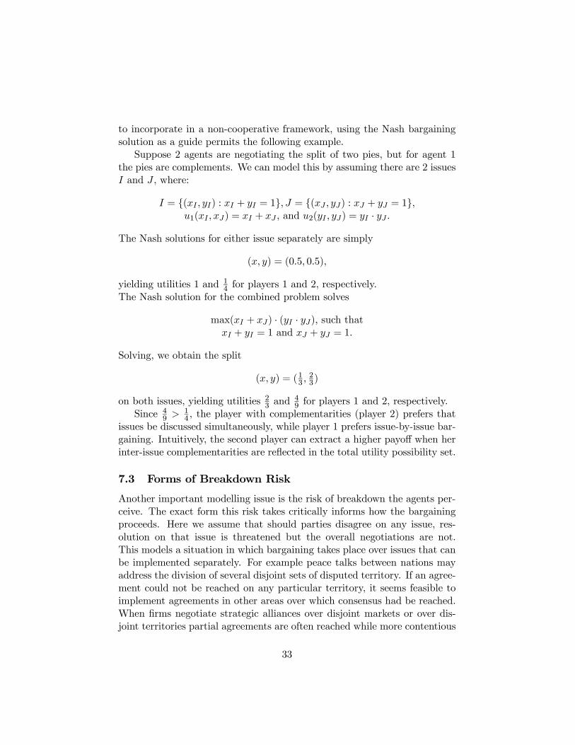
to incorporate in a non-cooperative framework, using the Nash bargainingsolution as a guide permits the following example.

Suppose 2 agents are negotiating the split of two pies, but for agent 1the pies are complements. We can model this by assuming there are 2 issuesI and J , where:

I = {(xI , yI) : xI + yI = 1}, J = {(xJ , yJ) : xJ + yJ = 1},u1(xI , xJ) = xI + xJ , and u2(yI , yJ) = yI · yJ .

The Nash solutions for either issue separately are simply

(x, y) = (0.5, 0.5),

yielding utilities 1 and 14 for players 1 and 2, respectively.

The Nash solution for the combined problem solves

max(xI + xJ) · (yI · yJ), such thatxI + yI = 1 and xJ + yJ = 1.

Solving, we obtain the split

(x, y) = (13 ,23)

on both issues, yielding utilities 23 and49 for players 1 and 2, respectively.

Since 49 > 1

4 , the player with complementarities (player 2) prefers thatissues be discussed simultaneously, while player 1 prefers issue-by-issue bar-gaining. Intuitively, the second player can extract a higher payoff when herinter-issue complementarities are reflected in the total utility possibility set.

7.3 Forms of Breakdown Risk

Another important modelling issue is the risk of breakdown the agents per-ceive. The exact form this risk takes critically informs how the bargainingproceeds. Here we assume that should parties disagree on any issue, res-olution on that issue is threatened but the overall negotiations are not.This models a situation in which bargaining takes place over issues that canbe implemented separately. For example peace talks between nations mayaddress the division of several disjoint sets of disputed territory. If an agree-ment could not be reached on any particular territory, it seems feasible toimplement agreements in other areas over which consensus had be reached.When firms negotiate strategic alliances over disjoint markets or over dis-joint territories partial agreements are often reached while more contentious

33

proposals remain unimplemented. When two people are deciding where toeat dinner and what movie to watch, it may be possible for them to eatseparately but still meet up to see a movie.

In contrast, many situations provide issues over which separate imple-mentation of agreements is not possible; an example being the labor problemmentioned earlier. Generally, a firm and a worker must agree on all majoraspects of a job before they can legally contract on the terms of employment.Two firms considering a joint venture may have to agree on every aspect be-fore the project becomes feasible. A car dealer and customer must decideon a model, options package, and financing before trade can take place. Inall of these examples failure to reach agreement on any issue produces thedisagreement outcome over all the issues.

7.4 Differing Risks

Finally, the assumption of one β across players and issues is easily relaxedwithout substantively changing our equilibrium analysis. Most naturally,some issue may be more volatile then others, with disagreements leadingmuch more readily to the collapse of talks. These issues would providelarger first-mover advantages and hence tend to be broached sooner thenless controversial issues. This may seem counterintuitive; in many real-worldnegotiations more volatile issues are often addressed latter. This could bemodeled as a time-varying β; issues broached latter may be less likely tobreak down due to a built up of good-faith between the bargainers. Oftenthough, issue are seen as volatile when the set of agreements both partieswould prefer to the status quo is very small; a feature which would encour-aging latter discussion since it would reduce first-mover surpluses.

8 Appendix: Proof of Equilibrium Uniqueness

Theorem 3 If monotonic strategies s01 and s02 are subgame-perfect, all is-sues must be settled exactly as in s1 and s2, our equilibrium strategies fromProposition 1, where

Definition 7 Strategies s01 and s02 are Monotonic if and only if:

For every state X, if ∃ a history h which leads to state X and afterwhich player j rejects player −j’s offer xI ∈ I with probability p > 0, thenafter every state X 0 such that:

1. X and X 0 differ only on issue I,

34

2. player −j also made the standing offer x0I ∈ I in X 0, and

3. player j likes xI strictly more then x0I (uj(xI) > uj(x0I)),

player j must reject −j0s offer on I.

Remark 5 Note that this is significantly weaker then the stationarity foundin the existing literature. Monotonicity requires only that holding all otherissues constant, a worse offer from −i to i on an issue makes i more likelyto reject that offer.

Proof of Theorem 3 We prove equilibrium uniqueness by iterated con-ditional dominance.

The proof of our main result proceeds as follows. We first establish thatin equilibrium the set of offers that can be made and the set that can berejected are very small. We then show that constrained to actions withinthese sets, the order issues can be broached is generically unique and givesrise to the same agreements.

Proceeding then, we first prove:

Lemma 3 (Restriction of Strategies) If Monotonic strategies s01 and s02

are subgame-perfect, then on any issue K, player j cannot:

1. offer an x ∈ K such that uj(x) < uj(rjK), or

2. accept an x ∈ K such that uj(x) < βuj(rjK),

if ∀L 6= K and L still open, ui(xiL) < ui(riL).

In words, no player can offer strictly less then her Rubinstein solution (whatshe offers in the single-issue case), or accept anything which is worse for himthen her opponent’s Rubinstein solution if all other standing offers do notask for strictly more then their Rubinstein values.

Proof of Lemma 3 For expositional simplicity I prove the Lemma in the2 issue case; the proof extends easily by identical arguments to the n issuecase.

Assume players are bargaining over 2 issues, I and J , and recall BiI

denotes the best outcome for agent i on issue I. Without loss of generalitywe focus on issue I; let f(x) be the function which maps player 1’s utilityto the highest utility player 2 can earn on I when 1 earns x; i.e.

35

f(x) = max{y : (x, y) ∈ I}.

Now assume the state of the game is < x1I , x1J >, i.e. no issue has broken

down, and for both issues the standing offer x was made by player 1. Furtherassume that

∀S, u2(x1S) > βu2(B2S).

In words, assume that 1 has offered 2 more then β times 2’s best possibleoutcome on every issue. Note that this is a possible subgame of the bar-gaining game for any number of issues; player 1 can make offer x1I on I,2 can propose on J , and then player 1 can reject and propose x2J . Sinceevery standing offer was made by player 1, it must be player 2’s turn in thissubgame.

Now in any SPE, player 2 cannot reject on I. Why? Rejecting on Icannot help on I, since the probability of breakdown already negates anypossible gains on I from rejecting.

Further, rejecting on I cannot help on J . Why? Any change to thestate of issue J would involve a risk of breakdown on that issue; hence 2 hasnothing to gain on any issue other then I. Switching the roles of the twoissues, we see that:

Conclusion 1 In such a state player 2 cannot reject on I, and must acceptboth issues.

Furthermore, if the state is < x2I , x1J >, it is 1’s turn,

u1(x2I) < βf−1(βu2(B2I )), andu2(x

1J) > βu2(B

2J),

then in any SPE player 1 cannot accept x2I . Why? Player 1 could reject x2I

and propose and agreement on I arbitrarily close to (f−1(βu2(B2I )), βu2(B2I )),

which by our first conclusion player 2 must accept. This earns player 1 apayoff of βf−1(βu2(B2I )) on issue I and leaves all other payoffs the same.

Conclusion 2 Hence in such a state player 1 can never accept such a x2I .

But note then that in state < x1I , x1J > where

u2(x1I) > βf(βf−1(βu2(B2I ))), and∀S 6= I, u2(x1S) > βu2(B

2S),

36

player 2 cannot reject on I. Why?By the same argument which established our first conclusion, if player 2

rejects x1I ,

1. 1will not accept any offer which gives him less then βf−1(βu2(B2I )),and

2. if she rejects will not propose anything which earns him less thenf−1(βu2(B2I ).

In either case 2 will not earn more then accepting x1I .Further, player 2 cannot reject on J . Why? If player 2 rejects and

counter-proposes on J either:

1. player 1 accepts player 2’s proposal, or

2. player 1 rejects player 2’s proposal and counter-proposes.

If the first happens, 2 has been hurt on J and by the original Rubinsteinargument must immediately accept x1I . If the second happens it cannot havehelped 2 on J . Could it have helped on issue I? Only if 1’s counter-proposalx is weakly worse for 2 then βu2(B

2J). But

βu2(B2J) ≥ u2(x)⇒ u2(x

1J) > u2(x).

But then by Monotonicity player 2 must immediately reject i’s counter-proposal x. Hence player 2 cannot act on I while the state is < x1I , y

1J >,

whenever

u2(y1J) ≤ βu2(B

2J).

But in both of these situations player 2 is strictly worse off.

Conclusion 3 Hence in such a state player 2 cannot reject x1I , and mustaccept both issues.

Now assume that we have shown that whenever player 1 has made bothpending offers, player 2 must accept both offers immediately if they arestrictly better for 2 then (mI ,mJ), with

u2(mI) ≥ u2(r1I ) and u2(mJ) ≥ u2(r

1J).

We now show 2 claims:

37

Claim 1 If the state is < x1I , x1J >, where:

1. u2(x1I) > βf(βf−1(mI)), and

2. u2(x1J) > mJ ,

then player 2 must accept both issues, and

Claim 2 if the state is < x2I , x1J >, it is 1’s turn,

u1(x2I) < βf−1(mI), andu2(x

1J) > mJ ,

then in any SPE player 1 must reject x2I .To establish these claims first note that if the state is < x2I , x

1J >, it is

1’s turn,

u1(x2I) < βf−1(mI), and u2(x

1J) > mj ,

then in any SPE player 1 cannot accept x2I . Why? Just as before player 1could reject x2I and propose and agreement on I arbitrarily close to (f

−1(mI),mI),which by our first conclusion 2 must accept. This earns player 1 a payoff ofβf−1(mI) on issue I and leaves all other payoffs the same.

But then player 1 cannot accept on issue I.This proves Claim 2. ¤Now towards our first claim; can player 1 reject on issue J? No, since if

player 2 rejects and counter-proposes on J either:

1. player 1 accepts player 2’s proposal, or

2. player 1 rejects player 2’s proposal and counter-proposes.

If the first happens, 2 has been hurt on J , and by the original Rubinsteinargument must immediately accept x1I . If the second happens it cannot havehelped 2 on J .

Can it have helped on issue I? Only if 1’s counter-proposal x is weaklyworse for 2 then mJ . But

mJ ≥ u2(x)⇒ u2(x1J) > u2(x).

But then by Monotonicity player 2 must then reject i’s counter-proposal x.Hence player 2 cannot act on I while the state is < x1I , y

1J >, whenever

38

u2(y1J) ≤ mj .

But in both of these situations player 2 is strictly worse off.This proves Claim 1. ¤Iterating the preceding arguments and noting that our selection of issue

I came without loss of generality, we arrive at the following conclusions:

Conclusion 4 Player 1 cannot accept x2K ∈ K ∈ {I, J} if

u1(x2K) < βf−1(βf(βf−1(βf(βf−1(...βf(βf−1(βu2(B2K)))...))))),

and ∀L 6= K and L open,u2(x

1−K) > βf(βf−1(βf(βf−1(...βf(βf−1(βu2(B2−K)))...)))).

Similarly,

Conclusion 5 Player 2 must immediately accept both x1K and x1−K if

u2(x1K) > βf(βf−1(βf(βf−1(...βf(βf−1(βu2(B2K)))...)))),

and ∀L 6= K and L open,u2(x

1−K) > βf−1(βf(βf−1(βf(βf−1(...βf(βf−1(βu2(B2−K)))...))))).

And as an immediate consequence,

Conclusion 6 Player 1 cannot propose x1K ∈ K where

u1(x1K) < f−1(βf(βf−1(βf(βf−1(...βf(βf−1(βu2(B2K)))...))))),

if ∀L 6= K and L open,u2(x

1−K) > βf−1(βf(βf−1(βf(βf−1(...βf(βf−1(βu2(B2−K)))...))))).

But note that these conditions converge to Rubinstein solutions, i.e.

βf−1(βf(βf−1(βf(βf−1(...βf(βf−1(βu2(B2K)))...))))) −→ u1(r2K),

andβf(βf−1(βf(βf−1(...βf(βf−1(βu2(B2K)))...)))) −→ u2(r

1K).

Finally, note that we can repeat these arguments with players 1 and 2switched, and recall the choice of I came without loss of generality.

Then these last three conclusions imply Lemma 3. ¤Now we use Lemma 3 to limit the types of outcomes that can occur in

equilibrium.

Lemma 4 (No Extreme Advantage) If Monotonic strategies s01 and s02are subgame-perfect, then players can not settle on < x̄I , x̄J >,14 whereui(xI) > ui(r

iI) and ui(xJ) > ui(r

iJ).

14Recall that an overbar denotes a final agreement.

39

Figure 8: Rubinstein solutions and the iterative process.

Proof of Lemma 4 We proceed by contradiction.Without loss of generality, we assume it is player 1 who has received

better then her Rubinstein values on both issues.By the original Rubinstein argument player 1must have gone last. With-

out loss of generality let us assume issue I settled last, at time t.This implies that player 2 moved at time t− 1, and must have moved on

issue J , since if not J must have already settled and player 2 could not haveoffered 1 better then her Rubinstein payoff on I (by subgame-perfection.)Continuing, player 1 moved at time t − 2, necessarily on issue J (else shecould not have closed issue I at time t.) Now without loss of generality,subgame-perfection lets us focus on equilibrium paths of the form:

< ..., x2I , x1J , x̄

2J , x̄

1I >.

But note that

u2(x2I) < u2(r

2I ),

yet 2 accepts and offer x1J such that

u2(x2J) < βu2(r

2J).

This violates Lemma 3, a contradiction.This proves Lemma 4. ¤

40

Remark 6 Note that it also cannot be the case that ui(xI) > ui(r1I ) and

ui(xJ) = ui(r1J), or vice-versa. Player 2 could have changed her time t − 1

move to revising her offer on issue I to arbitrarily close to r2I , which byLemma 3 would then have been accepted. This would have earned 2 a strictlyhigher payoff.

Finally, we prove that all payoffs that can be realized under some MSPEmust be bounded by the two Rubinstein payoffs on each issue. In otherwords,

Lemma 5 (No Extreme Payoffs) If Monotonic strategies s01 and s02 aresubgame-perfect, then players can not settle on < x̄I , x̄J >, where ui(xI) >ui(r

1I ) and uj(xJ) > uj(r

1J).

Proof of Lemma 5 As with Lemma 4, we can impose a tremendousamount of structure on the end of the equilibrium path without loss of gen-erality.

First note that if i = j, then we are done by Lemma 4. Toward acontradiction, assume that:

u1(x̄I) > u1(r1I ) and u2(x̄J) > u2(r

2J).

Without loss of generality, let player 1 have moved last. Again, subgame-perfection implies issue I must have settled last. Backward-constructing theequilibrium path, we arrive at:

< ..., x2I , x1J , x̄

2J , x̄

1I >.

But note that player 1 could have accepted player 2’s offer on issue I im-mediately. This would strictly increase 1’s payoff, since she would then geta minimum of

u1(r2J) = βu1(r

1I )

on issue J . This contradicts subgame-perfection.This proves Lemma 5. ¤But from Lemmas 3 − 5 it is immediate that only very specific equi-

librium paths are possible. Whenever a player proposes she must proposeher Rubinstein solution for that issue, and this can not be rejected by heropponent. The way Section 3.4 characterizes my solution is precisely thebackwards-inductive process both players face when they are restricted to

41

these types of offers and know their opponent is as well. Hence the so-lution characterized in this paper is generically unique among monotonesubgame-perfect equilibria of the multi-issue bargaining game. Note thatmixed strategies were not ruled out ex-ante, but are ruled out by the MSPErefinement.

This proves Theorem 3. ¤

References

[1] Binmore,K., Rubinstein, A., and Wolinsky, A. (1986), “The Nash Bar-gaining Solution in Economic Modelling,” Rand Journal of Economics17, 176-188

[2] Busch, L.A., and Horstmann, I.J. (1997), “Bargaining Frictions, Bar-gaining Procedures and Implied Costs in Multiple-Issue Bargaining,”Economica 64, 669-680

[3] Fershtman, C. (1990), “The Importance of the Agenda in Bargaining,”Games and Economic Behavior 2, 224-238

[4] Fudenberg, D. and Tirole, J. (1991) “Game Theory,” MIT Press, Cam-bridge, MA

[5] In, Y. and Serrano, R. (2001), “Agenda Restrictions in Multi-IssueBargaining,” mimeo

[6] Inderst, R. (2000), “Multi-Issue Bargaining with Endogenous Agenda,”Games and Economic Behavior 30, 64-82

[7] Maskin, E. and Tirole, J. (1988) “A Theory of Dynamic Oligopoly, II:Price Competition, Kinked Demand Curves, and Edgeworth Cycles,”Econometrica 56, 571-599

[8] Nash, J. (1950) “The Bargaining Problem,” Econometrica 18, 155-162

[9] O’Neill, B., Samet, D., Wiener, Z., and Winter, E. (2001), “Bargainingwith an Agenda,” mimeo

[10] Perry, M. and Reny, P. (1994) “A Noncooperative View of CoalitionFormation and the Core,” Econometrica 62, 795-817

[11] Raiffa, H. (1982), “The Art and Science of Negotiation,” Harvard Uni-versity Press, Cambridge, MA

42

[12] Rubinstein, A. (1982), “Perfect Equilibrium in a Bargaining Model,”Econometrica 50, 97-109

[13] Weinberger, C. (2000), “Selective Acceptance and Inefficiency in a Two-Issue Complete Information Bargaining Game,” Games and EconomicBehavior 31, 262-293

[14] Winter, E. (1997), “Negotiations in Multi-Issue Committees,” Journalof Public Economics 65, 323-342

43