Embed Size (px)
Citation preview
Aerodynamic Shape Optimization of Airfoils in
Ultra-Low Reynolds Number Flow using
Simultaneous Pseudo-Time Stepping
S. B. Hazra, A. Jameson
Aerospace Computing Lab (ACL) Report, 2007-4,
2007
1
Aerodynamic Shape Optimization of Airfoils in
Ultra-Low Reynolds Number Flow using
Simultaneous Pseudo-Time Stepping
S. B. Hazra1, A. Jameson2
1 Department of Mathematics, University of Trier, D-54286 Trier, Germany
2 Department of Aeronautics and Astronautics, Stanford University, Stanford,
CA 94305, USA
Abstract. The paper presents numerical results of optimized airfoils at ultra-low
Reynolds numbers. These investigations are carried out to understand the aerodynamic
issues related to the low speed and micro scale air vehicle design and performance. The
optimization method used is based on simultaneous pseudo-time stepping in which sta-
tionary states are obtained by solving the preconditioned pseudo-stationary system of
equations representing the state, costate and design equations. Design examples of airfoils
of different thicknesses at Mach numbers between 0.25 to 0.3 and at Reynolds numbers
below 15000 are presented.
1 Introduction
Aerodynamic studies of low Reynolds number flows have begun to take momentum. This
is due to the fact that technological advances have made it possible to consider Micro Air
Vehicles (MAVs) for various difficult missions of interest.
Aerodynamic studies are quite mature for flows with Reynolds number greater than
106. However, there are not many analytical or numerical or experimental studies available
for flows at very low Reynolds numbers. Consideration of 2d geometries, i.e., airfoils, for
such studies seems to be a good starting point to improve our understanding of low
Reynolds number flows. Some experimental studies are reported in [7, 8, 9]. Numerical
studies, for analysis as well as for design, and experimental validations of airfoils at ultra-
low Reynolds number are presented in [11, 12].
The viscous effects are dominant at low Reynolds numbers, and the flow physics
is quite complicated due to the predominance of separations. If the flow is laminar, a
2
separation bubble is formed in the boundary layer on the upper surface of the airfoil at
a quite low lift coefficient. The position of this bubble depends on the Reynolds number
and the angle of attack. These are also the parameters which determine weather the flow
reattaches behind the bubble or remains separated. If the flow remains separated, there
is a a sharp drop in the lift coefficient and an increase in the drag coefficient, leading to
a drastic reduction in the performance.
The paper is organized as follows. In the next section we give a brief description of
the numerical method used in this study. Section 3 presents the numerical results and
discussions. We draw our conclusions in Section 4.
2 Computational framework for simulation and op-
timization of the flow
The flow conditions that we considered are in the Mach numbers between 0.3 and 0.25 and
the Reynolds numbers less than 15000. The flow is assumed to be laminar. The SYN103
code of A. Jameson [5, 6, 4] has been used for the simulation and optimization which
is capable of running in laminar as well as in turbulent mode. The Reynolds averaged
Navier-Stokes equations together with the turbulence model of Baldwin and Lomax is
used for the flow modelling. The cell-centered finite volume method together with the
artificial dissipation of Jameson, Schmidt and Turkel is used in this code. For the time
stepping it uses 5 stage, 4th order Runge-Kutta type of scheme. The code additionally
has acceleration techniques such as multigrid, enthalpy damping and residual averaging.
It has been used for numerous applications in analysis and design, specially in transonic
flows.
The simultaneous pseudo-time stepping optimization method has been developed in
[1]. In this method the preconditioned pseudo-stationary system of equations resulting
from the necessary optimality conditions of the optimization problem are solved using time
stepping method. The preconditioner used in this method stems from the reduced SQP
methods. This method has been integrated into SYN103 code and used for optimization
in viscous transonic flow in [2]. In this work we use the same method and the code for
optimization at the very low Reynolds numbers. The code seems to work quite well in
these flow conditions.
3
3 Numerical results and discussion
The numerical method is applied to 2D test cases for drag reduction with constant lift
and constant thickness. The computational domain is discretized using 512 × 64 C-grid.
On this grid pseudo-unsteady state, costate and design equations are solved using the
SYN103 code. All the points on the airfoil are used as design parameters which are 257
in numbers.
Case 1: RAE 2822 airfoil at Reynolds number 15000
In this case the optimization method is applied to a RAE2822 airfoil at Mach number
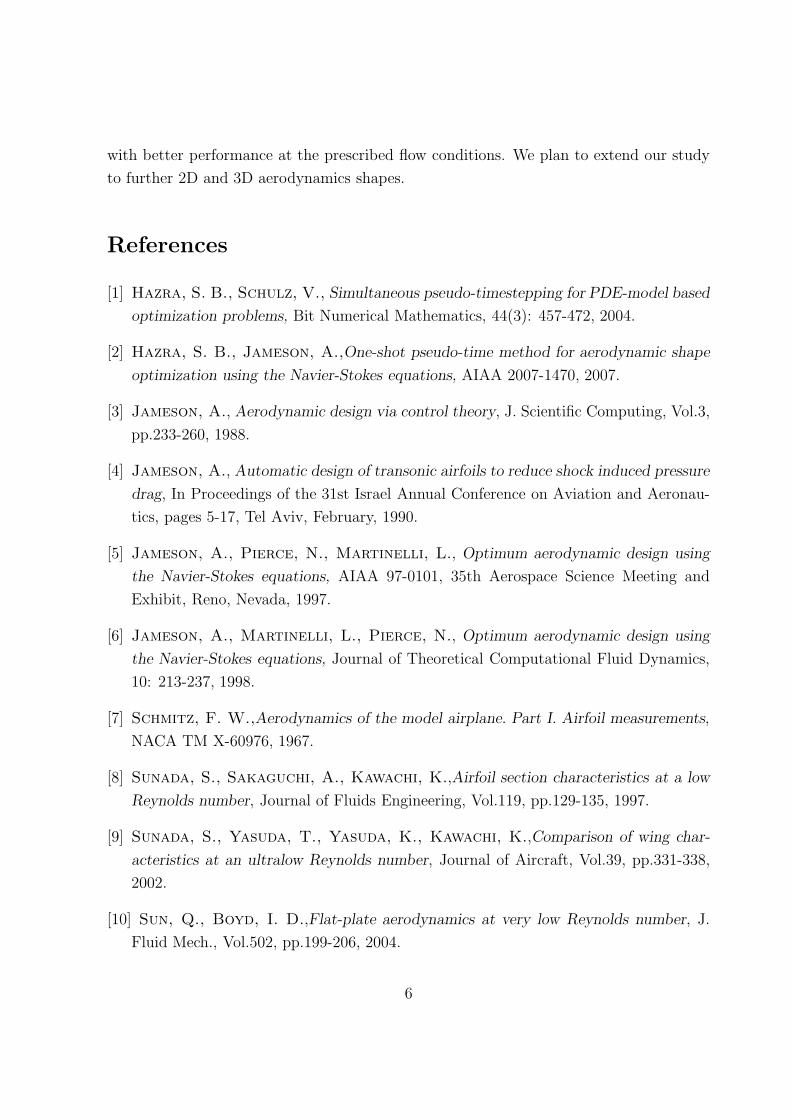
0.25. The constraint of constant lift coefficient is fixed at 0.2. Figure 1 presents the
cordwise pressure distribution (left) and the Mach contours (right) in baseline. As one
can see there is a separation bubble near the upper surface trailing edge of the airfoil.
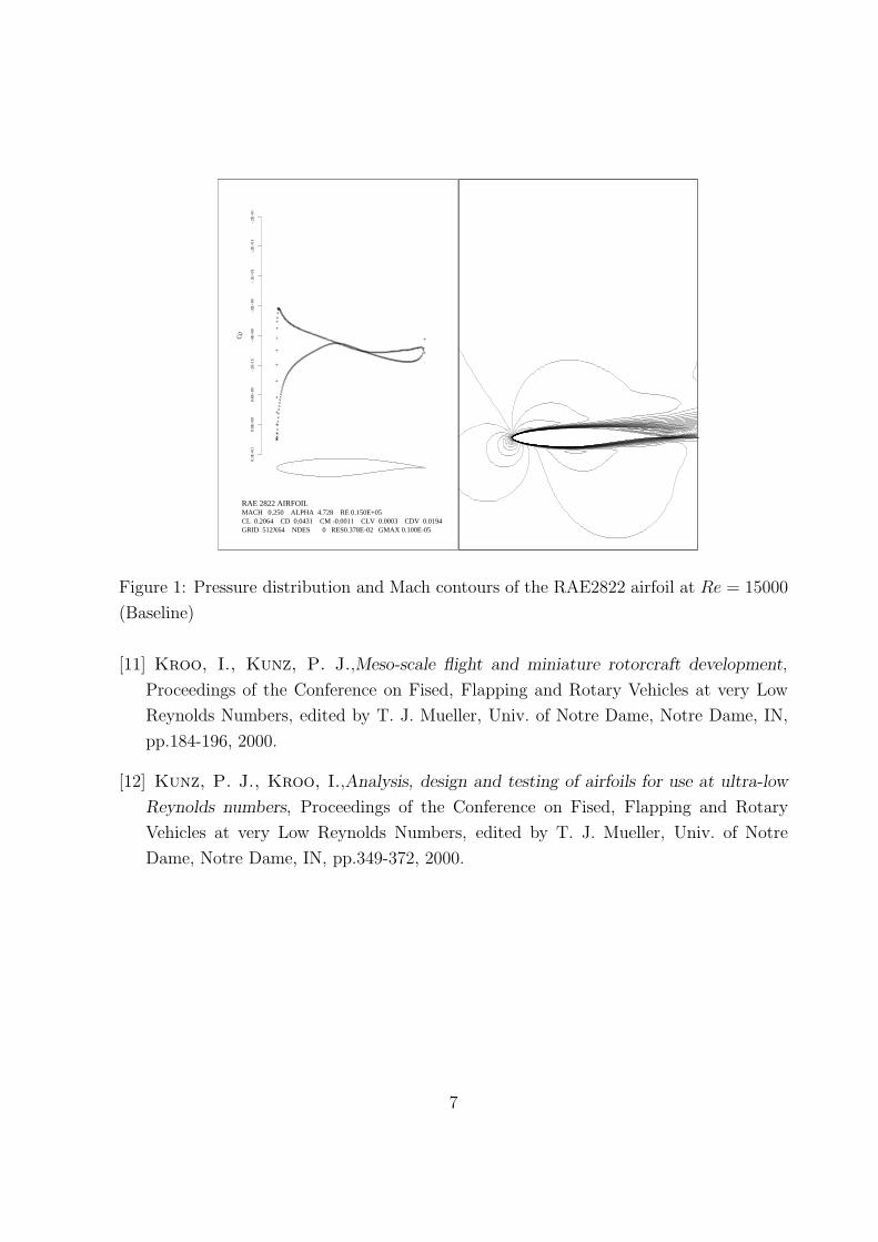
Figure 2 presents the vector plots of the velocity where, in the zoomed trailing edge, one
can clearly see the circulation zone forming the separation bubble. In Figures 3 and 4
the optimized surface pressure, Mach contours and the velocity vectors are presented. In
the optimized profiles the separation bubble has been disappeared making the flow purely
attached laminar one. The total drag, which is the sum of pressure drag and the viscous
drag, has been reduced by 82 counts. The values of the force coefficients are given in
Table 1.
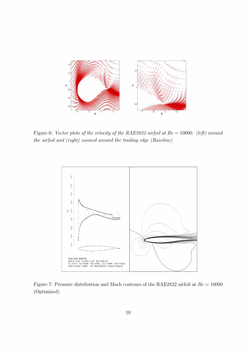
Case 3: RAE 2822 airfoil at Reynolds number 10000
In this case the optimization method is applied to a RAE2822 airfoil at Mach number 0.25.
The constraint of constant lift coefficient is fixed at 0.3. The reduction of Reynolds number
results in stronger separation bubble and hence larger drag value. Figure 5 presents the
cordwise pressure distribution and Mach contours. Figure 6 presents the vector plots of
the velocity. One can see the stronger separation bubble near the upper surface trailing
edge. The same optimized quantities are presented in Figures 7 and 8. The optimization
again has resulted the airfoil with attached laminar flow. The total drag in this case has
been reduced by about 170 counts. In both of these cases the viscous drag have been
increased by 8 and 22 counts respectively. The baseline and optimized force coefficients
are presented in Table 1. The polars are presented in Figure 9. As we can see there, the
optimized airfoil will have better performance around the lift coefficient upto 0.4.
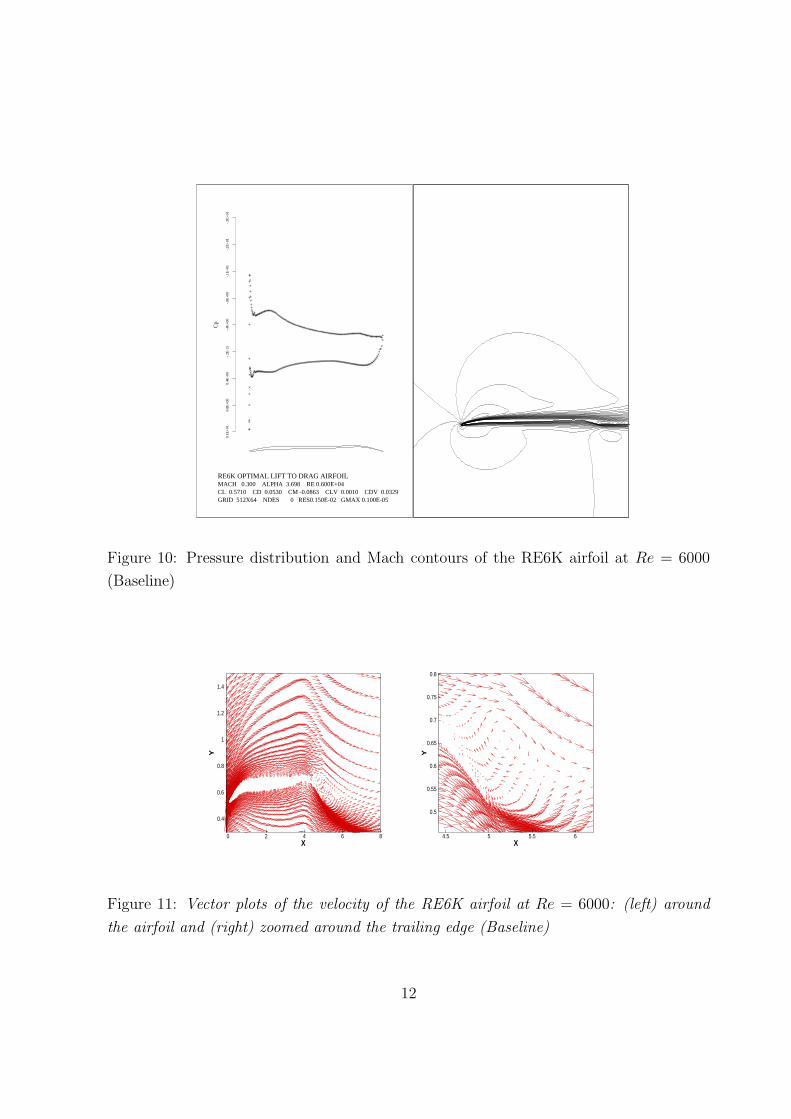
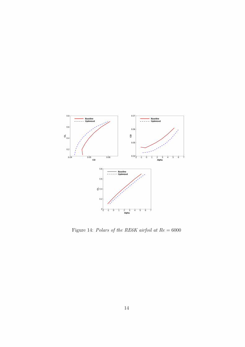
Case 3: RE6K airfoil at Reynolds number 6000
It is generally believed that thin airfoils perform better than thick airfoils at low Reynolds
numbers. In [12] the RE6K airfoil was optimized using a numerical method. The INS2D
code, where the incompressible fluid model is used, was used for that design. The airfoil
4
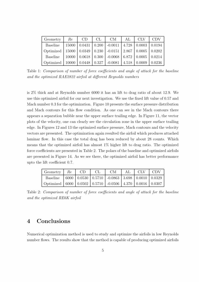
Geometry Re CD CL CM AL CLV CDV
Baseline 15000 0.0431 0.200 -0.0011 4.728 0.0003 0.0194
Optimized 15000 0.0349 0.230 -0.0151 2.867 0.0005 0.0202
Baseline 10000 0.0618 0.300 -0.0068 6.872 0.0005 0.0214
Optimized 10000 0.0448 0.327 -0.0081 4.518 0.0009 0.0236
Table 1: Comparison of number of force coefficients and angle of attack for the baseline
and the optimized RAE2822 airfoil at different Reynolds numbers
is 2% thick and at Reynolds number 6000 it has an lift to drag ratio of about 12.9. We
use this optimized airfoil for our next investigation. We use the fixed lift value of 0.57 and
Mach number 0.3 for the optimization. Figure 10 presents the surface pressure distribution
and Mach contours for this flow condition. As one can see in the Mach contours there
appears a separation bubble near the upper surface trailing edge. In Figure 11, the vector
plots of the velocity, one can clearly see the circulation zone in the upper surface trailing
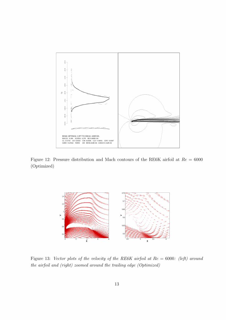
edge. In Figures 12 and 13 the optimized surface pressure, Mach contours and the velocity
vectors are presented. The optimization again resulted the airfoil which produces attached
laminar flow. In this case the total drag has been reduced by about 28 counts. Which
means that the optimized airfoil has almost 1% higher lift to drag ratio. The optimized
force coefficients are presented in Table 2. The polars of the baseline and optimized airfoils
are presented in Figure 14. As we see there, the optimized airfoil has better performance
upto the lift coefficient 0.7.
Geometry Re CD CL CM AL CLV CDV
Baseline 6000 0.0530 0.5710 -0.0863 3.698 0.0010 0.0329
Optimized 6000 0.0502 0.5710 -0.0506 4.370 0.0016 0.0307
Table 2: Comparison of number of force coefficients and angle of attack for the baseline
and the optimized RE6K airfoil
4 Conclusions
Numerical optimization method is used to study and optimize the airfoils in low Reynolds
number flows. The results show that the method is capable of producing optimized airfoils
5
with better performance at the prescribed flow conditions. We plan to extend our study
to further 2D and 3D aerodynamics shapes.
References
[1] Hazra, S. B., Schulz, V., Simultaneous pseudo-timestepping for PDE-model based
optimization problems, Bit Numerical Mathematics, 44(3): 457-472, 2004.
[2] Hazra, S. B., Jameson, A.,One-shot pseudo-time method for aerodynamic shape
optimization using the Navier-Stokes equations, AIAA 2007-1470, 2007.
[3] Jameson, A., Aerodynamic design via control theory, J. Scientific Computing, Vol.3,
pp.233-260, 1988.
[4] Jameson, A., Automatic design of transonic airfoils to reduce shock induced pressure
drag, In Proceedings of the 31st Israel Annual Conference on Aviation and Aeronau-
tics, pages 5-17, Tel Aviv, February, 1990.
[5] Jameson, A., Pierce, N., Martinelli, L., Optimum aerodynamic design using
the Navier-Stokes equations, AIAA 97-0101, 35th Aerospace Science Meeting and
Exhibit, Reno, Nevada, 1997.
[6] Jameson, A., Martinelli, L., Pierce, N., Optimum aerodynamic design using
the Navier-Stokes equations, Journal of Theoretical Computational Fluid Dynamics,
10: 213-237, 1998.
[7] Schmitz, F. W.,Aerodynamics of the model airplane. Part I. Airfoil measurements,
NACA TM X-60976, 1967.
[8] Sunada, S., Sakaguchi, A., Kawachi, K.,Airfoil section characteristics at a low
Reynolds number, Journal of Fluids Engineering, Vol.119, pp.129-135, 1997.
[9] Sunada, S., Yasuda, T., Yasuda, K., Kawachi, K.,Comparison of wing char-
acteristics at an ultralow Reynolds number, Journal of Aircraft, Vol.39, pp.331-338,
2002.
[10] Sun, Q., Boyd, I. D.,Flat-plate aerodynamics at very low Reynolds number, J.
Fluid Mech., Vol.502, pp.199-206, 2004.
6
RAE 2822 AIRFOIL MACH 0.250 ALPHA 4.728 RE 0.150E+05CL 0.2064 CD 0.0431 CM -0.0011 CLV 0.0003 CDV 0.0194GRID 512X64 NDES 0 RES0.378E-02 GMAX 0.100E-05
0.1E
+01
0.8E
+00
0.4E
+00
-.2E
-15
-.4E
+00
-.8E
+00
-.1E
+01
-.2E
+01
-.2E
+01
Cp
++++++++++++++++++++++++++++++++++++++++++++++++++
+++++++++++++++
++++++++++++++++++
+++++++++++++++++++++++++++++++++++++++++++++++++++++++++++++++++++++++++++
+
+
+
+
+
+
+
+
+++++++++++++++++++++++++++++++++++++++++++++++++++++++++++++++++++++++++++++++++++++++++++++++++++++++++++++++++++++++++++++++++++++++++++
+++++++++++++++
+
Figure 1: Pressure distribution and Mach contours of the RAE2822 airfoil at Re = 15000
(Baseline)
[11] Kroo, I., Kunz, P. J.,Meso-scale flight and miniature rotorcraft development,
Proceedings of the Conference on Fised, Flapping and Rotary Vehicles at very Low
Reynolds Numbers, edited by T. J. Mueller, Univ. of Notre Dame, Notre Dame, IN,
pp.184-196, 2000.
[12] Kunz, P. J., Kroo, I.,Analysis, design and testing of airfoils for use at ultra-low
Reynolds numbers, Proceedings of the Conference on Fised, Flapping and Rotary
Vehicles at very Low Reynolds Numbers, edited by T. J. Mueller, Univ. of Notre
Dame, Notre Dame, IN, pp.349-372, 2000.
7
X
Y
0 2 4 6
0.4
0.6
0.8
1
1.2
1.4
X
Y
4.5 5 5.5
0.8
1
1.2
Figure 2: Vector plots of the velocity of the RAE2822 airfoil at Re = 15000: (left) around
the airfoil and (right) zoomed around the trailing edge (Baseline)
RAE 2822 AIRFOIL MACH 0.250 ALPHA 2.867 RE 0.150E+05CL 0.2300 CD 0.0349 CM -0.0150 CLV 0.0005 CDV 0.0202GRID 512X64 NDES 120 RES0.270E-02 GMAX 0.144E-02
0.1E
+01
0.8E
+00
0.4E
+00
-.2E
-15
-.4E
+00
-.8E
+00
-.1E
+01
-.2E
+01
-.2E
+01
Cp
+++++++++++++++++++++++++++++++++++++++++
++++++++++++++++++
+++++++++++++
+++++++++++++++++++++++++++++++++++++++++++++++++++++++++++++++++++++++++
+++++
+++++++++
+
+
+
+
+
+
+
+++++
+++++++++++++++++++++++++++++++++++++++++++++++++++++++++++++++++++++++++++++++++++++++++++++++++++++++++++++++++++++++++++++++++++++++++++++++++++++
+
(a)
Figure 3: Pressure distribution and Mach contours of the RAE2822 airfoil at Re = 15000
(Optimized)
8
X
Y
0 2 4 6
0.4
0.6
0.8
1
1.2
1.4
X
Y
4.5 5 5.5
0.8
0.9
1
1.1
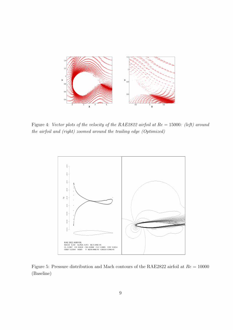
Figure 4: Vector plots of the velocity of the RAE2822 airfoil at Re = 15000: (left) around
the airfoil and (right) zoomed around the trailing edge (Optimized)
RAE 2822 AIRFOIL MACH 0.250 ALPHA 6.872 RE 0.100E+05CL 0.2967 CD 0.0618 CM -0.0068 CLV 0.0005 CDV 0.0214GRID 512X64 NDES 0 RES0.488E-03 GMAX 0.100E-05
0.1E
+01
0.8E
+00
0.4E
+00
-.2E
-15
-.4E
+00
-.8E
+00
-.1E
+01
-.2E
+01
-.2E
+01
Cp
+++++++++++++++++++++++++++++++++++++++++++++++++++++++++
+++++++++++++++++++
++++++++++++++++++++++++++++++++++++++++++++++++++++++++++++++++++++++++++++++++
++
+
+
+
+
+
+
+
+
+++++++++++++++++++++++++++++++++++++++++++++++++++++++++++++++++++++++++++++++++++++++++++++++++++++++++++++++++++++
+++++++++++++++++++++++++++++++++++++
+
Figure 5: Pressure distribution and Mach contours of the RAE2822 airfoil at Re = 10000
(Baseline)
9
X
Y
0 2 4 6
0.4
0.6
0.8
1
1.2
1.4
X
Y
4 4.5 5 5.5
0.8
1
1.2
Figure 6: Vector plots of the velocity of the RAE2822 airfoil at Re = 10000: (left) around
the airfoil and (right) zoomed around the trailing edge (Baseline)
RAE 2822 AIRFOIL MACH 0.250 ALPHA 4.518 RE 0.100E+05CL 0.3271 CD 0.0448 CM -0.0081 CLV 0.0009 CDV 0.0236GRID 512X64 NDES 120 RES0.385E-02 GMAX 0.166E-02
0.1E
+01
0.8E
+00
0.4E
+00
-.2E
-15
-.4E
+00
-.8E
+00
-.1E
+01
-.2E
+01
-.2E
+01
Cp
+++++++++++++++++++++++++++++++++++++++++++++++++
+++++++++++++++++
+++++++++++++++++++++++++++++++++++++++++++++++++++++++++++++++++++++++++++++++
++++++++++++
++
+
+
+
+
+
+
+
++++++++++++++++++++++++++++++++++++++++++++++++++++++++++++++++++++++++++++++++++++++++++++++++++++++++++++++++++++++++++++
++++++++++++++++++++++++++++++
+
Figure 7: Pressure distribution and Mach contours of the RAE2822 airfoil at Re = 10000
(Optimized)
10

X
Y
0 2 4 6
0.4
0.6
0.8
1
1.2
1.4
X
Y
4 4.5 5 5.5
0.8
1
Figure 8: Vector plots of the velocity of the RAE2822 airfoil at Re = 10000: (left) around
the airfoil and (right) zoomed around the trailing edge (Optimized)
CD
CL
0.03 0.045 0.06 0.075 0.09
0.15
0.225
0.3
0.375
0.45
BaselineOptimized
Alpha
CD
1 2 3 4 5 6 7 8 90.03
0.04
0.05
0.06
0.07
0.08
0.09
BaselineOptimized
Alpha
CL
1 2 3 4 5 6 7 8 90
0.1
0.2
0.3
0.4
0.5
BaselineOptimized
Figure 9: Polars of the RAE2822 airfoil at Re = 10000
11
RE6K OPTIMAL LIFT TO DRAG AIRFOIL MACH 0.300 ALPHA 3.698 RE 0.600E+04CL 0.5710 CD 0.0530 CM -0.0863 CLV 0.0010 CDV 0.0329GRID 512X64 NDES 0 RES0.150E-02 GMAX 0.100E-05
0.1E
+01
0.8E
+00
0.4E
+00
-.2E
-15
-.4E
+00
-.8E
+00
-.1E
+01
-.2E
+01
-.2E
+01
Cp
+++++
++++++++++++++++++++++++++++++++++++++++++++++++++++++++++++++++++++++++++++++++++++++++++++++++++++++++++++++++++++++++++++++++++++++++++++++++
++++++
+
+
+
++
+
+
+
+
+
+++++++++++++++++++++++++++++
+++++++++++++++++++++++++++++++++++++++++++++++++++++++++++++++++++++++++++++++++++++++++++++++++++++++++++++++++++++++++++++++
Figure 10: Pressure distribution and Mach contours of the RE6K airfoil at Re = 6000
(Baseline)
X
Y
0 2 4 6 8
0.4
0.6
0.8
1
1.2
1.4
X
Y
4.5 5 5.5 6
0.5
0.55
0.6
0.65
0.7
0.75
0.8
Figure 11: Vector plots of the velocity of the RE6K airfoil at Re = 6000: (left) around
the airfoil and (right) zoomed around the trailing edge (Baseline)
12
RE6K OPTIMAL LIFT TO DRAG AIRFOIL MACH 0.300 ALPHA 4.370 RE 0.600E+04CL 0.5710 CD 0.0502 CM -0.0506 CLV 0.0016 CDV 0.0307GRID 512X64 NDES 100 RES0.434E-04 GMAX 0.142E-02
0.1E
+01
0.8E
+00
0.4E
+00
-.2E
-15
-.4E
+00
-.8E
+00
-.1E
+01
-.2E
+01
-.2E
+01
Cp
+++++++++++++++++++++++++++++++++++++++++++++++++++++++++++++++++++++++++++++++++++++++++++++++++++++++++++++++++++++++++++++++++++++++++++++++++++++++++++
+
+
+++
+
+
+
+
+
+
+
+++
+
+
++++++++++++++++++++++++++++++++++++++++++++++++++++++++++++++++++++++++++++++++++++++++++++++++++++++++++++++++++++++++++++++++++++++++++++++++++++
+
Figure 12: Pressure distribution and Mach contours of the RE6K airfoil at Re = 6000
(Optimized)
X
Y
0 2 4 6 8
0.4
0.6
0.8
1
1.2
1.4
X
Y
4.5 5 5.5 6
0.5
0.55
0.6
0.65
0.7
0.75
Figure 13: Vector plots of the velocity of the RE6K airfoil at Re = 6000: (left) around
the airfoil and (right) zoomed around the trailing edge (Optimized)
13
CD
CL
0.04 0.05 0.06
0.2
0.4
0.6
0.8BaselineOptimized
Alpha
CD
-2 -1 0 1 2 3 4 5 6 70.04
0.05
0.06
0.07BaselineOptimized
Alpha
CL
-2 -1 0 1 2 3 4 5 6 70
0.2
0.4
0.6
0.8BaselineOptimized
Figure 14: Polars of the RE6K airfoil at Re = 6000
14


![Aerodynamic Optimization Trade Study of a Box-Wing ...oddjob.utias.utoronto.ca/~dwz/Miscellaneous/gagnonzingg...only supercritical airfoils are selected [18]. Specifically, for the](https://img.dokumen.tips/doc/110x75/5ac15cd07f8b9a357e8c96b3/aerodynamic-optimization-trade-study-of-a-box-wing-dwzmiscellaneousgagnonzinggonly.jpg)