Embed Size (px)
Citation preview

AERO 422: Active Controls for Aerospace VehiclesFrequency Response-Design Method
Raktim Bhattacharya
Intelligent Systems Research LaboratoryAerospace Engineering, Texas A&M University.

Frequency Response

Frequency Response Fourier Analysis Bode Plot Asymptotes Steady-State Stability Design
Response to Sinusoidal InputP
u(t) y(t)
Let u(t) = Au sin(ωt)Vary ω from 0 to ∞
A linear system’s response to sinusoidal inputs is called the system’s frequency response
AERO 422, Instructor: Raktim Bhattacharya 3 / 51

Frequency Response Fourier Analysis Bode Plot Asymptotes Steady-State Stability Design
Response to Sinusoidal InputExample
Let P (s) = 1s+1 , u(t) = sin(t)
y(t) =1
2e−t − 1
2cos(t) + 1
2sin(t)
=1
2e−t︸ ︷︷ ︸
natural response
+1√2
sin(t− π
4)︸ ︷︷ ︸
forced response
Forced response has form Ay sin(ωt+ ϕ)
Ay and ϕ are functions of ω
AERO 422, Instructor: Raktim Bhattacharya 4 / 51

Frequency Response Fourier Analysis Bode Plot Asymptotes Steady-State Stability Design
Response to Sinusoidal InputGeneralization
In general
Y (s) = G(s)ω0
s2 + ω20
=α1
s− p1+ · · · αn
s− pn+
α0
s+ jω0+
α∗0
s− jω0
=⇒ y(t) = α1ep1t + · · ·+ αne
pnt︸ ︷︷ ︸natural
+Ay sin(ω0 + ϕ)︸ ︷︷ ︸forced
Forced response has same frequency, different amplitude and phase.
AERO 422, Instructor: Raktim Bhattacharya 5 / 51

Frequency Response Fourier Analysis Bode Plot Asymptotes Steady-State Stability Design
Response to Sinusoidal InputGeneralization (contd.)
For a system P (s) and inputu(t) = Au sin(ω0t),
forced response isy(t) = AuM sin(ω0t+ ϕ),
where
M(ω0) = |P (s)|s=jω0 = |P (jω0)|,magnitude
ϕ(ω0) = P (jω0) phase
In polar formP (jω0) = Mejϕ.
AERO 422, Instructor: Raktim Bhattacharya 6 / 51

Fourier Analysis

Frequency Response Fourier Analysis Bode Plot Asymptotes Steady-State Stability Design
Fourier Series ExpansionGiven a signal y(t) with periodicity T ,
y(t) =a02
+∑
n=1,2,···an cos
(2πnt
T
)+ bn sin
(2πnt
T
)
a0 =2
T
∫ T
0y(t)dt
an =2
T
∫ T
0y(t) cos
(2πnt
T
)dt
bn =2
T
∫ T
0y(t) sin
(2πnt
T
)dt
AERO 422, Instructor: Raktim Bhattacharya 8 / 51

Frequency Response Fourier Analysis Bode Plot Asymptotes Steady-State Stability Design
Fourier Series ExpansionApproximation of step function
0 0.5 1 1.5 2 2.5 3 3.5 4 4.5 5−0.2
0
0.2
0.4
0.6
0.8
1
1.2
N=2
0 0.5 1 1.5 2 2.5 3 3.5 4 4.5 5−0.2
0
0.2
0.4
0.6
0.8
1
1.2
N=6
0 0.5 1 1.5 2 2.5 3 3.5 4 4.5 5−0.2
0
0.2
0.4
0.6
0.8
1
1.2
N=8
0 0.5 1 1.5 2 2.5 3 3.5 4 4.5 5−0.2
0
0.2
0.4
0.6
0.8
1
1.2
N=10
0 0.5 1 1.5 2 2.5 3 3.5 4 4.5 5−0.2
0
0.2
0.4
0.6
0.8
1
1.2
N=20
0 0.5 1 1.5 2 2.5 3 3.5 4 4.5 5−0.2
0
0.2
0.4
0.6
0.8
1
1.2
N=50
AERO 422, Instructor: Raktim Bhattacharya 9 / 51

Frequency Response Fourier Analysis Bode Plot Asymptotes Steady-State Stability Design
Fourier TransformStep function
Fourier transform reveals the frequency content of a signalAERO 422, Instructor: Raktim Bhattacharya 10 / 51

Frequency Response Fourier Analysis Bode Plot Asymptotes Steady-State Stability Design
Fourier TransformStep function – frequency content
0 0.2 0.4 0.6 0.8 1 1.2 1.4 1.6 1.8 2−0.2
0
0.2
0.4
0.6
0.8
1
1.2
t
y(t)
0 5 10 15 20 25 30 35 40 45 500
0.1
0.2
0.3
0.4
0.5
0.6
0.7
ω
y(ω
)
AERO 422, Instructor: Raktim Bhattacharya 11 / 51

Frequency Response Fourier Analysis Bode Plot Asymptotes Steady-State Stability Design
Signals & SystemsInput Output
Pu(t) y(t)
Fourier Series Expansionsuperposition principle
P∑
i ui(t)∑
i yi(t)
Fourier Transform
PU(jω) Y (jω)
ui(t) = ai sin(ωit)
yiforced(t) = aiM sin(ωit+ ϕ)
Y (jω) = P (jω)U(jω)
Suffices to study P (jω) |P (jω)|, P (jω)
AERO 422, Instructor: Raktim Bhattacharya 12 / 51

Bode Plot

Frequency Response Fourier Analysis Bode Plot Asymptotes Steady-State Stability Design
First Order System
−40
−35
−30
−25
−20
−15
−10
−5
0
Magnitude (
dB
)
10−2
10−1
100
101
102
−90
−45
0
Phase (
deg)
Bode Diagram
Frequency (rad/s)
P (s) = 1/(s+ 1)
loglog scaledB = 10 log10(·)20dB = 10 log10(100/1)
0 10 20 30 40 50 60 70 80 90 100−1
0
1
y(t)
Fre q = 0.10 rad/s
0 1 2 3 4 5 6 7 8 9 10−1
0
1
y(t)
Fre q = 1.00 rad/s
0 1 2 3 4 5 6 7 8 9 10−1
0
1
y(t)
Fre q = 5.00 rad/s
0 1 2 3 4 5 6 7 8 9 10−1
0
1
y(t)
Fre q = 10.00 rad/s
u(t) = A sin(ω0t)
yforced(t) = AM sin(ω0t+ ϕ)
AERO 422, Instructor: Raktim Bhattacharya 14 / 51

Frequency Response Fourier Analysis Bode Plot Asymptotes Steady-State Stability Design
Second Order System
−40
−30
−20
−10
0
10
Ma
gn
itu
de
(d
B)
10−1
100
101
−180
−135
−90
−45
0
Ph
ase
(d
eg
)
Bode Diagram
Frequency (rad/s)
P (s) = 1/(s2 + 0.5s+ 1)
ωn = 1 rad/s
0 10 20 30 40 50 60 70 80 90 100−2
0
2
y(t)
Fre q = 0.10 rad/s
0 10 20 30 40 50 60 70 80 90 100−2
0
2
y(t)
Fre q = 1.00 rad/s
0 1 2 3 4 5 6 7 8 9 10−1
0
1
y(t)
Fre q = 5.00 rad/s
0 1 2 3 4 5 6 7 8 9 10−1
0
1
y(t)
Fre q = 10.00 rad/s
u(t) = A sin(ω0t)
yforced(t) = AM sin(ω0t+ ϕ)
AERO 422, Instructor: Raktim Bhattacharya 15 / 51

Frequency Response Fourier Analysis Bode Plot Asymptotes Steady-State Stability Design
Lead Compensator
−15
−10
−5
0
5
10
Ma
gn
itu
de
(d
B)
10−2
10−1
100
101
102
103
0
30
60
Ph
ase
(d
eg
)
Lead Controller
Frequency (rad/s)
Phase leadlow gain at low frequencyhigh gain at high frequencyrelate it to derivative control
AERO 422, Instructor: Raktim Bhattacharya 16 / 51

Frequency Response Fourier Analysis Bode Plot Asymptotes Steady-State Stability Design
Lag Compensator
0
1
2
3
4
5
6
Ma
gn
itu
de
(d
B)
10−2
10−1
100
101
−20
−15
−10
−5
0
Ph
ase
(d
eg
)
Lag Controller
Frequency (rad/s)
Phase laghigh gain at low frequencylow gain at high frequencyrelate it to integral control
AERO 422, Instructor: Raktim Bhattacharya 17 / 51

Frequency Response Fourier Analysis Bode Plot Asymptotes Steady-State Stability Design
S(jω) + T (jω) = 1
10−2
10−1
100
101
102
10−2
10−1
100
101
ω rad/s
Magnitude|S
(jω)|
10−1
100
101
102
10−3
10−2
10−1
100
101
ω rad/s
Magnitude|T
(jω)|
C P+u+r +
d
+
n
e +y ym−ym
P (s) = 1(s+1)(s/2+1)
C(s) = 10
S = Ger = 11+PC
= 11+10P
T = Gyr = PC1+PC
= 10P1+10P
10−2
10−1
100
101
102
−60
−50
−40
−30
−20
−10
0
10
Magnitude (
dB
)
Bode Diagram
Frequency (rad/s)
S
T
S+T
AERO 422, Instructor: Raktim Bhattacharya 18 / 51

Frequency Response Fourier Analysis Bode Plot Asymptotes Steady-State Stability Design
All transfer functionsWith proportional controller
10−2
100
102
−30
−20
−10
0
10
Ma
gn
itu
de
(d
B)
Ger
Frequency (rad/s)
100
102
−80
−60
−40
−20
0
Ma
gn
itu
de
(d
B)
Ged
Frequency (rad/s)
10−2
100
102
−30
−20
−10
0
10
Ma
gn
itu
de
(d
B)
Gen
Frequency (rad/s)
100
102
−60
−40
−20
0
20
Ma
gn
itu
de
(d
B)
Gyr
Frequency (rad/s)
100
102
−80
−60
−40
−20
0
Ma
gn
itu
de
(d
B)
Gyd
Frequency (rad/s)
100
102
−60
−40
−20
0
20
Ma
gn
itu
de
(d
B)
Gyn
Frequency (rad/s)
AERO 422, Instructor: Raktim Bhattacharya 19 / 51

Frequency Response Fourier Analysis Bode Plot Asymptotes Steady-State Stability Design
Piper Dakota Control SystemDesigned with root locus method
SystemTransfer function from δe (elevator angle) to θ (pitch angle) is
P (s) =θ(s)
δe(s)=
160(s+ 2.5)(s+ 0.7)
(s2 + 5s+ 40)(s2 + 0.03s+ 0.06)
Control Objective 1Design an autopilot so that the step response to elevator input has tr < 1 andMp < 10% =⇒ ωn > 1.8 rad/s and ζ > 0.6 2nd order
Controller
C(s) = 1.5s+ 3
s+ 25(1 + 0.15/s)
AERO 422, Instructor: Raktim Bhattacharya 20 / 51

Frequency Response Fourier Analysis Bode Plot Asymptotes Steady-State Stability Design
Piper Dakota Control SystemTime Response
0 0.2 0.4 0.6−0.5
0
0.5
1
1.5
Ref to Control
Time (seconds)
Ele
va
tor
an
gle
(d
eg
)
0 10 20−0.5
0
0.5
1
Ref to Error
Time (seconds)
Err
or
(de
g)
0 10 200
0.5
1
1.5
Ref to Output
Time (seconds)
Pitch
An
gle
(d
eg
)
0 20 40−5
−4
−3
−2
−1
0
Dist to Error
Time (seconds)
Err
or
(de
g)
0 10 20−1.5
−1
−0.5
0
Dist to Control
Time (seconds)
Ele
va
tor
an
gle
(d
eg
)
0 20 400
1
2
3
4
5
Dist to Output
Time (seconds)
Pitch
an
gle
(d
eg
)AERO 422, Instructor: Raktim Bhattacharya 21 / 51

Frequency Response Fourier Analysis Bode Plot Asymptotes Steady-State Stability Design
Piper Dakota Control SystemFrequency Response
100
−80
−60
−40
−20
0
20
Ma
gn
itu
de
(d
B)
Ger
Frequency (rad/s)
100
−40
−30
−20
−10
0
10
20
Ma
gn
itu
de
(d
B)
Ged
Frequency (rad/s)
100
−80
−60
−40
−20
0
20
Ma
gn
itu
de
(d
B)
Gen
Frequency (rad/s)
100
−80
−60
−40
−20
0
20
Ma
gn
itu
de
(d
B)
Gyr
Frequency (rad/s)
100
−40
−30
−20
−10
0
10
20
Ma
gn
itu
de
(d
B)
Gyd
Frequency (rad/s)
100
−80
−60
−40
−20
0
20
Ma
gn
itu
de
(d
B)
Gyn
Frequency (rad/s)
AERO 422, Instructor: Raktim Bhattacharya 22 / 51

Frequency Response Fourier Analysis Bode Plot Asymptotes Steady-State Stability Design
Piper Dakota Control SystemFrequency Response (contd.)
10−2
10−1
100
101
102
103
−80
−60
−40
−20
0
20
Ma
gn
itu
de
(d
B)
Gur
Frequency (rad/s)
10−1
100
101
102
103
−80
−60
−40
−20
0
20
Ma
gn
itu
de
(d
B)
Gud
Frequency (rad/s)
AERO 422, Instructor: Raktim Bhattacharya 23 / 51

Asymptotes
Frequency Response Fourier Analysis Bode Plot Asymptotes Steady-State Stability Design
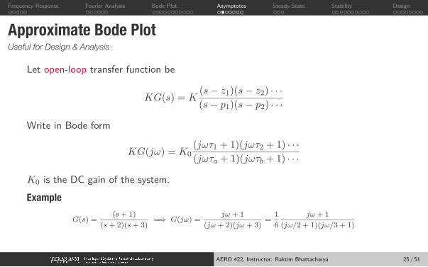
Approximate Bode PlotUseful for Design & Analysis
Let open-loop transfer function be
KG(s) = K(s− z1)(s− z2) · · ·(s− p1)(s− p2) · · ·
Write in Bode form
KG(jω) = K0(jωτ1 + 1)(jωτ2 + 1) · · ·(jωτa + 1)(jωτb + 1) · · ·
K0 is the DC gain of the system.Example
G(s) =(s+ 1)
(s+ 2)(s+ 3)=⇒ G(jω) =
jω + 1
(jω + 2)(jω + 3)=
1
6
jω + 1
(jω/2 + 1)(jω/3 + 1)
AERO 422, Instructor: Raktim Bhattacharya 25 / 51

Frequency Response Fourier Analysis Bode Plot Asymptotes Steady-State Stability Design
Approximate Bode Plotcontd.
Transfer function in Bode Form
KG(jω) = K0(jωτ1 + 1)(jωτ2 + 1) · · ·(jωτa + 1)(jωτb + 1) · · ·
Three cases1. K0(jω)
n pole, zero at origin
2. (jω + 1)±1 real pole, zero
3.[(
jωωn
)2+ 2ζ jω
ωn+ 1
]±1
complex pole, zero
AERO 422, Instructor: Raktim Bhattacharya 26 / 51

Frequency Response Fourier Analysis Bode Plot Asymptotes Steady-State Stability Design
Case:1 K0(jω)n
pole, zero at origin
GainlogK0|(jω)|n = logK0 + n log |jw| = logK0 + n logw
PhaseK0(jω)|n = K0 + n jω = 0 + n× 90◦
10−1
100
101
102
103
10−4
10−3
10−2
10−1
100
101
102
Bode Plot
Frequency (rad/s)
Gain
(a) Gain
10−1
100
101
102
103
−80
−60
−40
−20
0
20
40
60
80
Bode Plot
Frequency (rad/s)
Phase
(b) Phase
AERO 422, Instructor: Raktim Bhattacharya 27 / 51

Frequency Response Fourier Analysis Bode Plot Asymptotes Steady-State Stability Design
Case:2 (jωτ + 1)±1real pole, zero
Gain(jωτ + 1) =
{≈ 1, ωτ << 1,≈ jωτ, ωτ >> 1.
Frequency ω = 1/τ is the break point
10−1
100
101
102
103
10−4
10−3
10−2
10−1
100
101
102
Bode Plot
Frequency (rad/s)
Gain
AERO 422, Instructor: Raktim Bhattacharya 28 / 51

Frequency Response Fourier Analysis Bode Plot Asymptotes Steady-State Stability Design
Case:2 (jωτ + 1)±1real pole, zero (contd.)
Phase
jωτ + 1 =
≈ 1, ωτ << 1, 1 = 0◦
≈ jωτ, ωτ >> 1, jωτ = 90◦
ωτ ≈ 1, jωτ + 1 = 45◦
10−1
100
101
102
103
−80
−60
−40
−20
0
20
40
60
80
Bode Plot
Frequency (rad/s)
Phase
AERO 422, Instructor: Raktim Bhattacharya 29 / 51

Frequency Response Fourier Analysis Bode Plot Asymptotes Steady-State Stability Design
Example
G(s) =200(s+ 0.5)
s(s+ 10)(s+ 50)
−80
−60
−40
−20
0
20
40
Ma
gn
itu
de
(d
B)
10−2
10−1
100
101
102
103
−180
−135
−90
−45
0
Ph
ase
(d
eg
)
Bode Diagram
Frequency (rad/s)
Bode Diagram
Frequency (rad/s)
−80
−60
−40
−20
0
20
40
Ma
gn
itu
de
(d
B)
0.01 0.1 1 10 100 1000−180
−150
−120
−90
−60
−30
0
Ph
ase
(d
eg
)
AERO 422, Instructor: Raktim Bhattacharya 30 / 51

Steady-State Errors

Frequency Response Fourier Analysis Bode Plot Asymptotes Steady-State Stability Design
Closed-loop systemC Pu+r e y
−y
Closed-loop transfer functionGer =
1
1 + PC= K0(jω)
n (jωτ1 + 1)(jωτ2 + 1) · · ·(jωτa + 1)(jωτb + 1) · · ·
Steady-state gain
lims→0
sGer(s)1
s⇔ lim
ω→0|Ger(jω)|
PC =200(s+ 0.5)
s(s+ 10)(s+ 50)
Typically analysis is done with open-loop system
10−3
10−2
10−1
100
101
102
−60
−50
−40
−30
−20
−10
0
10
Magnitude (
dB
)
Bode Diagram
Frequency (rad/s)
AERO 422, Instructor: Raktim Bhattacharya 32 / 51

Frequency Response Fourier Analysis Bode Plot Asymptotes Steady-State Stability Design
Open-loop systemC Pu+r e y
−y
Open-loop transfer functionPC =
200(s+ 0.5)
s(s+ 10)(s+ 50)= K0(jω)
n (jωτ1 + 1)(jωτ2 + 1) · · ·(jωτa + 1)(jωτb + 1) · · ·
Steady-state error step
ess =1
1 +Kp, Kp := K0.
Steady-state error ramp
ess =1
Kv
System type is the slope of the low frequencyasymptoteKv is the value of low frequency asymptote atω = 1 rad/s 10
−210
−110
010
110
210
3−80
−60
−40
−20
0
20
40
Magnitude (
dB
)
Bode Diagram
Frequency (rad/s)
AERO 422, Instructor: Raktim Bhattacharya 33 / 51

Stability Analysis
Frequency Response Fourier Analysis Bode Plot Asymptotes Steady-State Stability Design
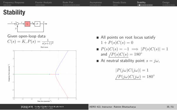
StabilityC Pu+r e y
−y
Given open-loop dataC(s) = K,P (s) = 1
s(s+1)2
−5 −4 −3 −2 −1 0 1 2−3
−2
−1
0
1
2
3
Root Locus
Real Axis (seconds−1
)
Imagin
ary
Axis
(seconds
−1)
Stable for K < 2
All points on root locus satisfy1 + P (s)C(s) = 0
P (s)C(s) = −1 =⇒ |P (s)C(s)| = 1and P (s)C(s) = 180◦
At neutral stability point s = jω,
|P (jω)C(jω)| = 1
P (jω)C(jω) = 180◦
AERO 422, Instructor: Raktim Bhattacharya 35 / 51

Frequency Response Fourier Analysis Bode Plot Asymptotes Steady-State Stability Design
Stability|P (jω)C(jω)| < 1 at P (jω)C(jω) = 180◦
−150
−100
−50
0
50
100
Magnitude (
dB
)
10−2
10−1
100
101
102
−270
−225
−180
−135
−90
−45
0
Phase (
deg)
Bode Diagram
Frequency (rad/s)
K=0.1
K=2
K=10
AERO 422, Instructor: Raktim Bhattacharya 36 / 51

Frequency Response Fourier Analysis Bode Plot Asymptotes Steady-State Stability Design
Gain MarginOpen loop Bode Plot
−150
−100
−50
0
50
100
Ma
gn
itu
de
(d
B)
10−2
10−1
100
101
102
−270
−225
−180
−135
−90
−45
0
Ph
ase
(d
eg
)
Bode Diagram
Frequency (rad/s)
K=0.1
K=2
K=10
Gain Margin (GM): factor by which gain can be increased at P (jω)C(jω) = −180◦
AERO 422, Instructor: Raktim Bhattacharya 37 / 51

Frequency Response Fourier Analysis Bode Plot Asymptotes Steady-State Stability Design
Phase MarginOpen loop Bode Plot
−150
−100
−50
0
50
100
Ma
gn
itu
de
(d
B)
10−2
10−1
100
101
102
−270
−225
−180
−135
−90
−45
0
Ph
ase
(d
eg
)
Bode Diagram
Frequency (rad/s)
K=0.1
K=2
K=10
Phase Margin (PM): amount by which phase exceeds −180◦ at |P (jω)C(jω)| = 1
AERO 422, Instructor: Raktim Bhattacharya 38 / 51

Frequency Response Fourier Analysis Bode Plot Asymptotes Steady-State Stability Design
Nyquist PlotRelates open-loop frequency response to number of unstable closed-loop polesResidue theorem in complex analysisPlot P (jω)C(jω) in the complex plainNumber of encirclements of −1 equals Z − P of 1 + P (s)C(s)
AERO 422, Instructor: Raktim Bhattacharya 39 / 51

Frequency Response Fourier Analysis Bode Plot Asymptotes Steady-State Stability Design
Nyquist Plotcontd.
Write P (s)C(s) = KG(s) = KN(s)D(s)
=⇒ 1 + P (s)C(s) =D(s) +KN(s)
D(s)
Poles of 1 + P (s)C(s) = Poles of G(s) none of them on RHP
Number of encirclements = number of zeros of 1 + P (s)C(s) on RHPnumber of poles of closed-loop system
AERO 422, Instructor: Raktim Bhattacharya 40 / 51

Frequency Response Fourier Analysis Bode Plot Asymptotes Steady-State Stability Design
Nyquist PlotExample: P (s)C(s) = K
s(s+1)2
−10 −5 0 5−3
−2
−1
0
1
2
3
Nyquist Diagram
Real Axis
Imagin
ary
Axis
K=1
K=2
K=10
AERO 422, Instructor: Raktim Bhattacharya 41 / 51

Frequency Response Fourier Analysis Bode Plot Asymptotes Steady-State Stability Design
Nyquist PlotDetermining Gain
Given P (s)C(s) = Ks(s+1)2
, what is K for stability?Encirclement of 1/K +G(s) = 0
−2 −1.8 −1.6 −1.4 −1.2 −1 −0.8 −0.6 −0.4 −0.2 0−2
−1.5
−1
−0.5
0
0.5
1
1.5
2
Nyquist Diagram
Real Axis
Imagin
ary
Axis
AERO 422, Instructor: Raktim Bhattacharya 42 / 51

Frequency Response Fourier Analysis Bode Plot Asymptotes Steady-State Stability Design
Nyquist PlotGain and Phase Margin
Nyquist plot of P (s)C(s)
−2 −1.5 −1 −0.5 0 0.5 1 1.5 2−2
−1.5
−1
−0.5
0
0.5
1
1.5
2
Nyquist Diagram
Real Axis
Imagin
ary
Axis
AERO 422, Instructor: Raktim Bhattacharya 43 / 51

Frequency Domain Design

Frequency Response Fourier Analysis Bode Plot Asymptotes Steady-State Stability Design
Design Using Bode Plot of P (jω)C(jω)Loop Shaping
Develop conditions on the Bode plot of the open loop transfer functionSensitivity 1
1+PC
Steady-state errors: slope and magnitude at limω → 0
Robust to sensor noiseDisturbance rejectionController roll off =⇒ not excite high-frequency modes of plantRobust to plant uncertainty
Look at Bode plot of L(jω) := P (jω)C(jw)
AERO 422, Instructor: Raktim Bhattacharya 45 / 51

Frequency Response Fourier Analysis Bode Plot Asymptotes Steady-State Stability Design
Frquency Domain SpecificationsConstraints on the shape of L(jω)
Stea
dy-s
tate
erro
r bou
ndar
y
Sens
or n
oise
, pla
nt
unce
rtain
ty
!!c
1
|P(j!)C
(j!)|
slope ⇡ 1
!!c
1
|P(j!)C
(j!)|
slope ⇡ 1
Steady-state error boundary
Sensor noise, disturbance Plant uncertainty
Choose C(jω) to ensure |L(jω)| does not violate the constraintsSlope ≈ −1 at ωc ensures PM ≈ 90◦ stable if PM > 0 =⇒ PC > −180◦
AERO 422, Instructor: Raktim Bhattacharya 46 / 51

Frequency Response Fourier Analysis Bode Plot Asymptotes Steady-State Stability Design
Plant UncertaintyP (jω) = P0(jω)(1 + ∆P (jω))
10−2
10−1
100
101
102
103
−250
−200
−150
−100
−50
0
50
Ma
gn
itu
de
(d
B)
Bode Diagram
Frequency (rad/s)
True
Model
Unc+
Unc−
Stea
dy-s
tate
erro
r bou
ndar
y
Sens
or n
oise
, pla
nt
unce
rtain
ty
!!c
1
|P(j!)C
(j!)|
slope ⇡ 1
!!c
1
|P(j!)C
(j!)|
slope ⇡ 1
Steady-state error boundary
Sensor noise, disturbance Plant uncertainty
AERO 422, Instructor: Raktim Bhattacharya 47 / 51

Frequency Response Fourier Analysis Bode Plot Asymptotes Steady-State Stability Design
Sensor CharacteristicsNoise spectrum
Stea
dy-s
tate
erro
r bou
ndar
y
Sens
or n
oise
, pla
nt
unce
rtain
ty
!!c
1
|P(j!)C
(j!)|
slope ⇡ 1
!!c
1
|P(j!)C
(j!)|
slope ⇡ 1
Steady-state error boundary
Sensor noise, disturbance Plant uncertainty
Gyn = − PC
1 + PC
AERO 422, Instructor: Raktim Bhattacharya 48 / 51

Frequency Response Fourier Analysis Bode Plot Asymptotes Steady-State Stability Design
Reference TrackingBandlimited else conflicts with noise rejection
0 5 10 15 20 25
0.01
0.02
0.03
0.04
0.05
Spectrum of r(t)
Frequency (Hz)
|X(f
)|
0 5 10 15 20 25
0.01
0.02
0.03
0.04
0.05
Spectrum of n(t)
Frequency (Hz)
|X(f
)|
Stea
dy-s
tate
erro
r bou
ndar
y
Sens
or n
oise
, pla
nt
unce
rtain
ty
!!c
1
|P(j!)C
(j!)|
slope ⇡ 1
!!c
1
|P(j!)C
(j!)|
slope ⇡ 1
Steady-state error boundary
Sensor noise, disturbance Plant uncertainty
Gyr =PC
1 + PC
Gyn = − PC1+PC
AERO 422, Instructor: Raktim Bhattacharya 49 / 51

Frequency Response Fourier Analysis Bode Plot Asymptotes Steady-State Stability Design
Disturbance RejectonBandlimited else conflicts with noise rejection
0 5 10 15 20 25
0.01
0.02
0.03
0.04
0.05
Spectrum of n(t)
Frequency (Hz)
|X(f
)|
0 5 10 15 20 25
0.01
0.02
0.03
0.04
0.05
Spectrum of d(t)
Frequency (Hz)
|X(f
)|
Stea
dy-s
tate
erro
r bou
ndar
y
Sens
or n
oise
, pla
nt
unce
rtain
ty
!!c
1
|P(j!)C
(j!)|
slope ⇡ 1
!!c
1
|P(j!)C
(j!)|
slope ⇡ 1
Steady-state error boundary
Sensor noise, disturbance Plant uncertainty
Gyd =P
1 + PC
Gyn = − PC1+PC
AERO 422, Instructor: Raktim Bhattacharya 50 / 51