Embed Size (px)
Citation preview

ADVANCED WATER DISTRIBUTION MODELING
AND MANAGEMENT
Authors
Thomas M. Walski
Donald V. Chase
Dragan A. Savic
Walter Grayman
Stephen Beckwith
Edmundo Koelle
Contributing Authors
Scott Cattran, Rick Hammond, Kevin Laptos, Steven G. Lowry,
Robert F. Mankowski, Stan Plante, John Przybyla, Barbara Schmitz
Peer Review Board
Lee Cesario (Denver Water), Robert M. Clark (U.S. EPA),
Jack Dangermond (ESRI), Allen L. Davis (CH2M Hill),
Paul DeBarry (Borton-Lawson), Frank DeFazio (Franklin G. DeFazio Corp.),
Kevin Finnan (Bristol Babcock), Wayne Hartell (Bentley Systems),
Brian Hoefer (ESRI), Bassam Kassab (Santa Clara Valley Water District),
James W. Male (University of Portland), William M. Richards
(WMR Engineering), Zheng Wu (Bentley Systems ),
and E. Benjamin Wylie (University of Michigan)
Click here to visit the Bentley Institute Press Web page for more information

C H A P T E R
3Assembling a Model
As Chapter 1 discusses, a water distribution model is a mathematical description of a real-world system. Before building a model, it is necessary to gather information describing the network. In this chapter, we introduce and discuss sources of data used in constructing models.
The latter part of the chapter covers model skeletonization. Skeletonization is the pro-cess of simplifying the real system for model representation, and it involves making decisions about the level of detail to be included.
3.1 MAPS AND RECORDSMany potential sources are available for obtaining the data required to generate a water distribution model, and the availability of these sources varies dramatically from utility to utility. The following sections discuss some of the most commonly used resources, including system maps, as-built drawings, and electronic data files.
System MapsSystem maps are typically the most useful documents for gaining an overall under-standing of a water distribution system because they illustrate a wide variety of valuable system characteristics. System maps may include such information as
• Pipe alignment, connectivity, material, diameter, and so on
• The locations of other system components, such as tanks and valves
• Pressure zone boundaries
• Elevations
• Miscellaneous notes or references for tank characteristics
• Background information, such as the locations of roadways, streams, plan-ning zones, and so on
• Other utilities

76 Assembling a Model Chapter 3
Topographic MapsA topographic map uses sets of lines called contours to indicate elevations of the ground surface. Contour lines represent a contiguous set of points that are at the same elevation and can be thought of as the outline of a horizontal “slice” of the ground sur-face. Figure 3.1 illustrates the cross-sectional and topographic views of a sphere, and Figure 3.2 shows a portion of an actual topographic map. Topographic maps are often referred to by the contour interval that they present, such as a 20-foot topographic map or a 1-meter contour map.
By superimposing a topographic map on a map of the network model, it is possible to interpolate the ground elevations at junction nodes and other locations throughout the system. Of course, the smaller the contour interval, the more precisely the elevations can be estimated. If available topographic maps cannot provide the level of precision needed, other sources of elevation data need to be considered.
Topographic maps are also available in the form of Digital Elevation Models (DEMs),which can be used to electronically interpolate elevations. The results of the DEM are only as accurate as the underlying topographic data on which they are based; thus, it is possible to calculate elevations to a large display precision but with no additional accuracy.
Figure 3.1Topographic representation of a hemisphere
Looking DownGeneratesPlan View
Profile
Plan
Looking fromthe Side
GeneratesProfile View
0
100
200
200100
0
400
300
300
400
As-Built Drawings
Site restrictions and on-the-fly changes often result in differences between original design plans and the actual constructed system. As a result, most utilities perform post-construction surveys and generate a set of as-built or record drawings for the purpose of documenting the system exactly as it was built. In some cases, an inspec-tor's notes may even be used as a supplemental form of documentation. As-built drawings can be especially helpful in areas where a fine level of precision is required for pipe lengths, fitting types and locations, elevations, and so forth.

Section 3.1 Maps and Records 77
Figure 3.2Typical topographic map
As-built drawings can also provide reliable descriptions of other system components such as storage tanks and pumping stations. There may be a complete set of drawings for a single tank, or the tank plans could be included as part of a larger construction project.
Electronic Maps and RecordsMany water distribution utilities have some form of electronic representation of their systems in formats that may vary from a nongraphical database, to a graphics-only Computer-Aided Drafting (CAD) drawing, to a Geographic Information System (GIS)that combines graphics and data.
Nongraphical Data. It is common to find at least some electronic data in non-graphical formats, such as a tracking and inventory database, or even a legacy text-based model. These sources of data can be quite helpful in expediting the process of model construction. Even so, care needs to be taken to ensure that the network topol-ogy is correct, because a simple typographic error in a nongraphical network can be difficult to detect.
Computer-Aided Drafting. The rise of computer technology has led to many improvements in all aspects of managing a water distribution utility, and mapping is no exception. CAD systems make it much easier to plug in survey data, combine data from different sources, and otherwise maintain and update maps faster and more reli-ably than ever before.

78 Assembling a Model Chapter 3
Even for systems having only paper maps, many utilities digitize those maps to con-vert them to an electronic drawing format. Traditionally, digitizing has been a process of tracing over paper maps with special computer peripherals, called a digitizing tab-let and puck (see Figure 3.3). A paper map is attached to the tablet, and the drafts- person uses crosshairs on the puck to point at locations on the paper. Through magnetic or optical techniques, the tablet creates an equivalent point at the appropriate location in the CAD drawing. As long as the tablet is calibrated correctly, it will automatically account for rotation, skew, and scale.
Figure 3.3A typical digitizing tablet
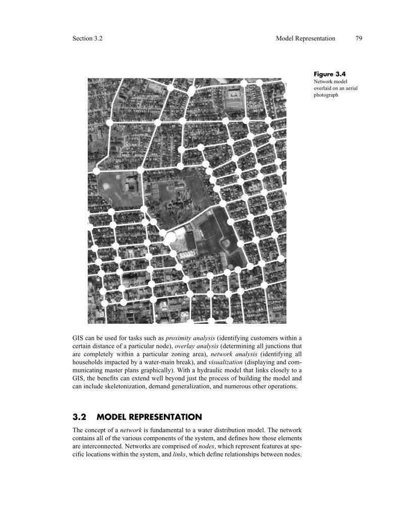
Another form of digitizing is called heads-up digitizing (see Figure 3.4). This method involves scanning a paper map into a raster electronic format (such as a bitmap), bringing it into the background of a CAD system, and electronically tracing over it on a different layer. The term heads-up is used because the draftsperson remains focused on the computer screen rather than on a digitizing tablet.
Geographic Information Systems. A Geographic information system (GIS) is a computer-based tool for mapping and analyzing objects and events that happen on earth. GIS technology integrates common database operations such as query and statistical analysis with the unique visualization and geographic analysis benefits offered by maps (ESRI, 2001). Because a GIS stores data on thematic layers linked together geographically, disparate data sources can be combined to determine relationships between data and to synthesize new information.
Section 3.2 Model Representation 79
Figure 3.4Network model overlaid on an aerial photograph
GIS can be used for tasks such as proximity analysis (identifying customers within a certain distance of a particular node), overlay analysis (determining all junctions that are completely within a particular zoning area), network analysis (identifying all households impacted by a water-main break), and visualization (displaying and com-municating master plans graphically). With a hydraulic model that links closely to a GIS, the benefits can extend well beyond just the process of building the model and can include skeletonization, demand generalization, and numerous other operations.
3.2 MODEL REPRESENTATIONThe concept of a network is fundamental to a water distribution model. The network contains all of the various components of the system, and defines how those elements are interconnected. Networks are comprised of nodes, which represent features at spe-cific locations within the system, and links, which define relationships between nodes.

80 Assembling a Model Chapter 3
Network ElementsWater distribution models have many types of nodal elements, including junction nodes where pipes connect, storage tank and reservoir nodes, pump nodes, and con-trol valve nodes. Models use link elements to describe the pipes connecting these nodes. Also, elements such as valves and pumps are sometimes classified as links rather than nodes. Table 3.1 lists each model element, the type of element used to rep-resent it in the model, and the primary modeling purpose.
Table 3.1 Common network modeling elements
Element Type Primary Modeling Purpose
Reservoir Node Provides water to the system
Tank Node Stores excess water within the system and releases that water at times of high usage
Junction Node Removes (demand) or adds (inflow) water from/to the system
Pipe Link Conveys water from one node to another
Pump Node or link
Raises the hydraulic grade to overcome elevation differences and friction losses
Control Valve
Node or link
Controls flow or pressure in the system based on specified criteria
Naming Conventions (Element Labels). Because models may contain tens of thousands of elements, naming conventions are an important consideration in mak-ing the relationship between real-world components and model elements as obvious as possible (see Figure 3.5). Some models allow only numeric numbering of ele-ments, but most modern models support at least some level of alphanumeric labeling (for example, “J-1,” “Tank 5,” or “West Side Pump A”).
Figure 3.5Schematic junction with naming convention
J5 - 115 - ElmStreet
Description“115” = Sequential Number
“5” = Zone 5“J” = Junction Node
Naming conventions should mirror the way the modeler thinks about the particular network by using a mixture of prefixes, suffixes, numbers, and descriptive text. In general, labels should be as short as possible to avoid cluttering a drawing or report, but they should include enough information to identify the element. For example, a naming convention might include a prefix for the element type, another prefix to indi-cate the pressure zone or map sheet, a sequential number, and a descriptive suffix.
Section 3.2 Model Representation 81
Of course, modelers can choose to use some creativity, but it is important to realize that a name that seems obvious today may be baffling to future users. Intelligent use of element labeling can make it much easier for users to query tabular displays of model data with filtering and sorting commands. In some cases, such as automated calibration, it may be very helpful to group pipes with like characteristics to make cal-ibration easier. If pipe labels have been set up such that like pipes have similar labels, this grouping becomes easy.
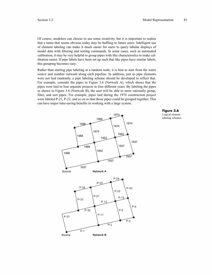
Rather than starting pipe labeling at a random node, it is best to start from the water source and number outward along each pipeline. In addition, just as pipe elements were not laid randomly, a pipe labeling scheme should be developed to reflect that. For example, consider the pipes in Figure 3.6 (Network A), which shows that the pipes were laid in four separate projects in four different years. By labeling the pipes as shown in Figure 3.6 (Network B), the user will be able to more rationally group, filter, and sort pipes. For example, pipes laid during the 1974 construction project were labeled P-21, P-22, and so on so that those pipes could be grouped together. This can have major time-saving benefits in working with a large system.
Figure 3.6Logical element labeling schemes
82 Assembling a Model Chapter 3
Boundary Nodes. A boundary node is a network element used to represent locations with known hydraulic grade elevations. A boundary condition imposes a requirement within the network that simulated flows entering or exiting the system agree with that hydraulic grade. Reservoirs (also called fixed grade nodes) and tanks are common examples of boundary nodes.
Every model must have at least one boundary node so that there is a reference point for the hydraulic grade. In addition, every node must maintain at least one path back to a boundary node so that its hydraulic grade can be calculated. When a node becomes disconnected from a boundary (as when pipes and valves are closed), it can result in an error condition that needs to be addressed by the modeler.
Network TopologyThe most fundamental data requirement is to have an accurate representation of the network topology, which details what the elements are and how they are intercon-nected. If a model does not faithfully duplicate real-world layout (for example, the model pipe connects two nodes that are not really connected), then the model will never accurately depict real-world performance, regardless of the quality of the remaining data.
System maps are generally good sources of topological information, typically includ-ing data on pipe diameters, lengths, materials, and connections with other pipes. There are situations in which the modeler must use caution, however, because maps may be imperfect or unclear.
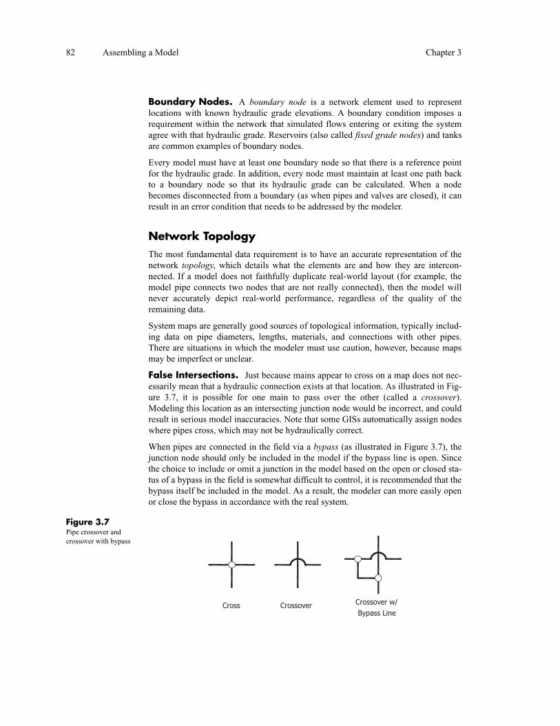
False Intersections. Just because mains appear to cross on a map does not nec-essarily mean that a hydraulic connection exists at that location. As illustrated in Fig-ure 3.7, it is possible for one main to pass over the other (called a crossover).Modeling this location as an intersecting junction node would be incorrect, and could result in serious model inaccuracies. Note that some GISs automatically assign nodes where pipes cross, which may not be hydraulically correct.
When pipes are connected in the field via a bypass (as illustrated in Figure 3.7), the junction node should only be included in the model if the bypass line is open. Since the choice to include or omit a junction in the model based on the open or closed sta-tus of a bypass in the field is somewhat difficult to control, it is recommended that the bypass itself be included in the model. As a result, the modeler can more easily open or close the bypass in accordance with the real system.
Figure 3.7Pipe crossover and crossover with bypass
Cross Crossover Crossover w/
Bypass Line

Section 3.2 Model Representation 83
Converting CAD Drawings into Models. Although paper maps can some-times falsely make it appear as though there is a pipe intersection, CAD maps can have the opposite problem. CAD drawings are often not created with a hydraulic model in mind; thus, lines representing pipes may visually appear to be connected on a large-scale plot, but upon closer inspection of the CAD drawing, the lines are not actually touching. Consider Figure 3.8, which demonstrates three distinct conditions that may result in a misinterpretation of the topology:
• T-intersections: Are there supposed to be three intersecting pipes or two non-intersecting pipes? The drawing indicates that there is no intersection, but this could easily be a drafting error.
• Crossing pipes: Are there supposed to be four intersecting pipes or two non-intersecting pipes?
• Nearly connecting line endpoints: Are the two pipes truly non-intersecting?
Automated conversion from CAD drawing elements to model elements can save time, but (as with any automated process) the modeler needs to be aware of the potential pitfalls involved and should review the end result. Some models assist in the review process by highlighting areas with potential connectivity errors. The possibility of difficult-to-detect errors still remains, however, persuading some modelers to trace over CAD drawings when creating model elements.

84 Assembling a Model Chapter 3
Figure 3.8Common CAD conversion errors
3.3 RESERVOIRSThe term reservoir has a specific meaning with regard to water distribution system modeling that may differ slightly from the use of the word in normal water distribu-tion construction and operation. A reservoir represents a boundary node in a model that can supply or accept water with such a large capacity that the hydraulic grade of the reservoir is unaffected and remains constant. It is an infinite source, which means that it can theoretically handle any inflow or outflow rate, for any length of time, without running dry or overflowing. In reality, there is no such thing as a true infinite source. For modeling purposes, however, there are situations where inflows and out-flows have little or no effect on the hydraulic grade at a node.
Reservoirs are used to model any source of water where the hydraulic grade is con-trolled by factors other than the water usage rate. Lakes, groundwater wells, and clearwells at water treatment plants are often represented as reservoirs in water distri-bution models. For modeling purposes, a municipal system that purchases water from a bulk water vendor may model the connection to the vendor’s supply as a reservoir (most current simulation software includes this functionality).
For a reservoir, the two pieces of information required are the hydraulic grade line (water surface elevation) and the water quality. By model definition, storage is not a concern for reservoirs, so no volumetric storage data is needed.
3.4 TANKSA storage tank (see Figure 3.9) is also a boundary node, but unlike a reservoir, the hydraulic grade line of a tank fluctuates according to the inflow and outflow of water. Tanks have a finite storage volume, and it is possible to completely fill or completely exhaust that storage (although most real systems are designed and operated to avoid such occurrences). Storage tanks are present in most real-world distribution systems, and the relationship between an actual tank and its model counterpart is typically straightforward.

Section 3.4 Tanks 85
Figure 3.9Storage tanks
For steady-state runs, the tank is viewed as a known hydraulic grade elevation, and the model calculates how fast water is flowing into or out of the tank given that HGL. Given the same HGL setting, the tank is hydraulically identical to a reservoir for a steady-state run. In extended-period simulation (EPS) models, the water level in the tank is allowed to vary over time. To track how a tank’s HGL changes, the relationship between water surface elevation and storage volume must be defined. Figure 3.10 illus-trates this relationship for various tank shapes. For cylindrical tanks, developing this relationship is a simple matter of identifying the diameter of the tank, but for non-cylindrical tanks it can be more challenging to express the tank’s characteristics.
Some models do not support noncylindrical tanks, forcing the modeler to approximate the tank by determining an equivalent diameter based on the tank’s height and capac-ity. This approximation, of course, has the potential to introduce significant errors in hydraulic grade. Fortunately, most models do support non-cylindrical tanks, although the exact set of data required varies from model to model.
Regardless of the shape of the tank, several elevations are important for modeling pur-poses. The maximum elevation represents the highest fill level of the tank, and is usually determined by the setting of the altitude valve if the tank is equipped with one. The overflow elevation, the elevation at which the tank begins to overflow, is slightly higher. Similarly, the minimum elevation is the lowest the water level in the tank should ever be. A base or reference elevation is a datum from which tank levels are measured.
The HGL in a tank can be referred to as an absolute elevation or a relative level,depending on the datum used. For example, a modeler working near the “Mile High” city of Denver, Colorado, could specify a tank’s base elevation as the datum, and then work with HGLs that are relative to that datum. Alternatively, the modeler could work with absolute elevations that are in the thousands of feet. The choice of whether to use absolute elevations or relative tank levels is a matter of personal preference. Figure

86 Assembling a Model Chapter 3
3.11 illustrates these important tank elevation conventions for modeling tanks. Notice that when using relative tank levels, it is possible to have different values for the same level, depending on the datum selected.
Figure 3.10Volume versus level curves for various tank shapes
Volu
me
Ratio
Depth Ratio
0 0.1 0.2 0.3 0.4 0.5 0.6 0.7 0.8 0.9 1.0
1.0
0.9
0.8
0.7
0.6
0.5
0.4
0.3
0.2
0.1
0
Spherical
45 Deg. Cone
Cylindrical/Rectangular
Water storage tanks can be classified by construction material (welded steel, bolted steel, reinforced concrete, prestressed concrete), shape (cylindrical, spherical, torroi-dal, rectangular), style (elevated, standpipe, ground, buried), and ownership (utility, private) (Walski, 2000). However, for pipe network modeling, the most important classification is whether or not the tank “floats on the system.” A tank is said to floaton the system if the hydraulic grade elevation inside the tank is the same as the HGL in the water distribution system immediately outside of the tank. With tanks, there are really three situations that a modeler can encounter:
1. Tank that floats on the system with a free surface
2. Pressure (hydropneumatic) tank that floats on the system
3. Pumped storage in which water must be pumped from a tank

Section 3.4 Tanks 87
Figure 3.11Important tank elevations
Figure 3.12 shows that elevated tanks, standpipes, and hydropneumatic tanks float on the system because their HGL is the same as that of the system. Ground tanks and buried tanks may or may not float on the system, depending on their elevation. If the HGL in one of these tanks is below the HGL in the system, water must be pumped from the tank, resulting in pumped storage.
A tank with a free surface floating on the system is the simplest and most common type of tank. The pumped storage tank needs a pump to deliver water from the tank to the distribution system and a control valve (usually modeled as a pressure sustaining valve) to gradually fill the tank without seriously affecting pressure in the surrounding system.
Figure 3.12Relationship between floating, pressurized, and pumped tanks
HGL
Elevated Standpipe
GroundBuried
Ground
Buried
Hydro-Pneumatic
//=//=
//=
//=
//=
//=
Pumped Storage Floating on System

88 Assembling a Model Chapter 3
Hydropneumatic Tanks. In most tanks, the water surface elevation in the tank equals the HGL in the tank. In the case of a pressure tank, however, the HGL is higher than the tank’s water surface. Pressure tanks, also called hydropneumatic tanks, are partly full of compressed air. Because the water in the tank is pressurized, the HGL is higher than the water surface elevation, as reflected in Equation 3.1.
HGL CfP Z+= (3.1)
where HGL = HGL of water in tank (ft, m)P = pressure recorded at tank (psi, kPa)Z = elevation of pressure gage (ft, m)Cf = unit conversion factor (2.31 English, 0.102 SI)
In steady-state models, a hydropneumatic tank can be represented by a tank or reser-voir having this HGL. In EPS models, the tank must be represented by an equivalent free-surface tank floating on the system. Because of the air in the tank, a hydropneu-matic tank has an effective volume that is less than 30 to 50 percent of the total volume of the tank. Modeling the tank involves first determining the minimum and maximum pressures occurring in the tank and converting them to HGL values using Equation 3.1. The cross-sectional area (or diameter) of this equivalent tank can be determined by using Equation 3.2.
AeqVeff
HGLmax HGLmin–------------------------------------------------= (3.2)
where Aeq = area of equivalent tank (ft2, m2)Veff = effective volume of tank (ft3, m3)
HGLmax = maximum HGL in tank (ft, m)HGLmin = minimum HGL in tank (ft, m)
The relationship between the actual hydropneumatic tank and the model tank is shown in Figure 3.13.
Using this technique, the EPS model of the tank will track HGL at the tank and vol-ume of water in the tank, but not the actual water level.
3.5 JUNCTIONSAs the term implies, one of the primary uses of a junction node is to provide a loca-tion for two or more pipes to meet. Junctions, however, do not need to be elemental intersections, as a junction node may exist at the end of a single pipe (typically referred to as a dead-end). The other chief role of a junction node is to provide a loca-tion to withdraw water demanded from the system or inject inflows (sometimes referred to as negative demands) into the system.
Junction nodes typically do not directly relate to real-world distribution components, since pipes are usually joined with fittings, and flows are extracted from the system at any number of customer connections along a pipe. From a modeling standpoint, the

Section 3.5 Junctions 89
importance of these distinctions varies, as discussed in the section on skeletonization on page 112. Most water users have such a small individual impact that their with-drawals can be assigned to nearby nodes without adversely affecting a model.
Figure 3.13Relationship between a hydropneumatic tank and a model tank
Veff
HGLmax
HGLmin
Pressure Tank
EquivalentModelTank
Veff
Pump off
Pump on
Pump
Junction Elevation
Generally, the only physical characteristic defined at a junction node is its elevation. This attribute may seem simple to define, but there are some considerations that need to be taken into account before assigning elevations to junction nodes. Because pres-sure is determined by the difference between calculated hydraulic grade and eleva-tion, the most important consideration is, at what elevation is the pressure most important?
Selecting an Elevation. Figure 3.14 represents a typical junction node, illus-trating that at least four possible choices for elevation exist that can be used in the model. The elevation could be taken as point A, the centerline of the pipe. Alterna-tively, the ground elevation above the pipe (point B), or the elevation of the hydrant (point C), may be selected. As a final option, the ground elevation at the highest ser-vice point, point D, could be used. Each of these possibilities has associated benefits, so the determination of which elevation to use needs to be made on a case-by-case basis. Regardless of which elevation is selected, it is good practice to be consistent within a given model to avoid confusion.

90 Assembling a Model Chapter 3
Figure 3.14Elevation choices for a junction node
//=//=
//=//=
//=//=
//=//=
//=//=//=//= //=//=//=//=
Pipe - A (622’)
Ground - B (630’)
High Service - D (650’)
HydrantElevation - C (635’)
ServiceLine
The elevation of the centerline of the pipe may be useful for determining pressure for leakage studies, or it may be appropriate when modeling above-ground piping sys-tems (such as systems used in chemical processing). Ground elevations may be the easiest data to obtain and will also overlay more easily onto mapping systems that use ground elevations. They are frequently used for models of municipal water distribu-tion systems. Both methods, however, have the potential to overlook poor service pressures because the model could incorrectly indicate acceptable pressures for a cus-tomer who is notably higher than the ground or pipe centerline. In such cases, it may be more appropriate to select the elevation based on the highest service elevation required.
In the process of model calibration (see Chapter 7 for more about calibration), accu-rate node elevations are crucial. If the elevation chosen for the modeled junction is not the same as the elevation associated with recorded field measurements, then direct pressure comparisons are meaningless. Methods for obtaining good node elevation data are described in Walski (1999).
3.6 PIPES
A pipe conveys flow as it moves from one junction node to another in a network. In the real world, individual pipes are usually manufactured in lengths of around 18 or 20 feet (6 meters), which are then assembled in series as a pipeline. Real-world pipe-lines may also have various fittings, such as elbows, to handle abrupt changes in direction, or isolation valves to close off flow through a particular section of pipe. Figure 3.15 shows ductile iron pipe sections.
For modeling purposes, individual segments of pipe and associated fittings can all be combined into a single pipe element. A model pipe should have the same characteris-tics (size, material, etc.) throughout its length.

Section 3.6 Pipes 91
Figure 3.15Ductile iron pipe sections
LengthThe length assigned to a pipe should represent the full distance that water flows from one node to the next, not necessarily the straight-line distance between the end nodes of the pipe.
Scaled versus Schematic. Most simulation software enables the user to indi-cate either a scaled length or a user-defined length for pipes. Scaled lengths are auto-matically determined by the software, or scaled from the alignment along an electronic background map. User-defined lengths, applied when scaled electronic maps are not available, require the user to manually enter pipe lengths based on some other measurement method, such as use of a map wheel (see Figure 3.16). A model using user-defined lengths is a schematic model. The overall connectivity of a sche-matic model should be identical to that of a scaled model, but the quality of the plani-metric representation is more similar to a caricature than a photograph.
Even in some scaled models, there may be areas where there are simply too many nodes in close proximity to work with them easily at the model scale (such as at a pump station). In these cases, the modeler may want to selectively depict that portion of the system schematically, as shown in Figure 3.17.
DiameterAs with junction elevations, determining a pipe’s diameter is not as straightforward as it might seem. A pipe’s nominal diameter refers to its common name, such as a 16-in. (400-mm) pipe. The pipe’s internal diameter, the distance from one inner wall of the pipe to the opposite wall, may differ from the nominal diameter because of manufac-turing standards. Most new pipes have internal diameters that are actually larger than the nominal diameters, although the exact measurements depend on the class (pres-sure rating) of pipe.

92 Assembling a Model Chapter 3
Figure 3.16Use of a map measuring wheel for measuring pipe lengths
Figure 3.17Scaled system with a schematic of a pump station
Scaled System
Pump Station Schematic(not to scale)
For example, Figure 3.18 depicts a new ductile iron pipe with a 16-in. nominal diam-eter (ND) and a 250-psi pressure rating that has an outside diameter (OD) of 17.40 in. and a wall thickness (Th) of 0.30 in., resulting in an internal diameter (ID) of 16.80 in. (AWWA, 1996).
To add to the confusion, the ID may change over time as corrosion, tuberculation, and scaling occur within the pipe (see Figure 3.19). Corrosion and tuberculation are related in iron pipes. As corrosion reactions occur on the inner surface of the pipe, the reaction by-products expand to form an uneven pattern of lumps (or tubercules) in a process called tuberculation. Scaling is a chemical deposition process that forms a material build-up along the pipe walls due to chemical conditions in the water. For

Section 3.6 Pipes 93
example, lime scaling is caused by the precipitation of calcium carbonate. Scaling can actually be used to control corrosion, but when it occurs in an uncontrolled manner it can significantly reduce the ID of the pipe.
Figure 3.18Cross-section of a 16-in. pipe
Figure 3.19Pipe corrosion and tuberculation
Courtesy of Donald V. Chase, Department of Civil Engineering, University of Dayton
Of course, no one is going to refer to a pipe as a 16.80-in. (426.72-mm) pipe, and because of the process just described, it is difficult to measure a pipe’s actual internal diameter. As a result, a pipe’s nominal diameter is commonly used in modeling, in combination with a roughness value that accounts for the diameter discrepancy. How-ever, using nominal rather than actual diameters can cause significant differences

94 Assembling a Model Chapter 3
when water quality modeling is performed. Because flow velocity is related to flow rate by the internal diameter of a pipe, the transport characteristics of a pipe are affected. Chapter 7 discusses these calibration issues further (see page 255). Typical roughness values can be found in Section 2.4.
Minor LossesIncluding separate modeling elements to represent every fitting and appurtenance present in a real-world system would be an unnecessarily tedious task. Instead, the minor losses caused by those fittings are typically associated with pipes (that is, minor losses are assigned as a pipe property).
In many hydraulic simulations, minor losses are ignored because they do not contrib-ute substantially to the overall head loss throughout the system. In some cases, however, flow velocities within a pipe and the configuration of fittings can cause minor losses to be considerable (for example, at a pump station). The term “minor” is relative, so the impact of these losses varies for different situations.
Red WaterDistribution systems with unlined iron or steel pipes can be subject to water quality problems related to corrosion, referred to as red water. Red water is treated water containing a colloidal sus-pension of very small, oxidized iron particles that originated from the surface of the pipe wall. Over a long period of time, this form of corrosion weak-ens the pipe wall and leads to the formation of tubercles. The most obvious and immediate impact, however, is that the oxidized iron particles give the water a murky, reddish-brown color. This reduction in the aesthetic quality of the water prompts numerous customer complaints.
Several alternative methods are available to con-trol the pipe corrosion that causes red water. The most traditional approach is to produce water that is slightly supersaturated with calcium carbonate. When the water enters the distribution system, the dissolved calcium carbonate slowly precipitates on the pipe walls, forming a thin, protective scale (Caldwell and Lawrence, 1953; Merrill and Sanks, 1978). The Langelier Index (an index of the corro-sive potential of water) can be used as an indica-tion of the potential of the water to precipitate calcium carbonate, allowing better management of the precipitation rate (Langelier, 1936).
A positive saturation index indicates that the pipe should be protected, provided that sufficient alka-linity is present.
More recently, corrosion inhibitors such as zinc orthophosphate and hexametaphosphate have become popular in red water prevention (Ben-jamin, Reiber, Ferguson, Vanderwerff, and Miller, 1990; Mullen and Ritter, 1974; Volk, Dundore, Schiermann, and LeChevallier, 2000). Several theories exist concerning the predominant mecha-nism by which these inhibitors prevent corrosion.
The effectiveness of corrosion control measures can be dependent on the hydraulic flow regime occurring in the pipe. Several researchers have reported that corrosion inhibitors and carbonate films do not work well in pipes with low velocities (Maddison and Gagnon, 1999; McNeil and Edwards, 2000). Water distribution models pro-vide a way to identify pipes with chronic low veloc-ities, and therefore more potential for red water problems. The effect of field operations meant to control red water (for example, flushing and blow-offs) can also be investigated using hydraulic model simulations.

Section 3.7 Pumps 95
Composite Minor Losses. At any instant in time, velocity in the model is con-stant throughout the length of a particular pipe. Since individual minor losses are related to a coefficient multiplied by a velocity term, the overall head loss from sev-eral minor losses is mathematically equivalent to having a single composite minor loss coefficient. This composite coefficient is equal to the simple sum of the individual coefficients.
3.7 PUMPSA pump is an element that adds energy to the system in the form of an increased hydraulic grade. Since water flows “downhill” (that is, from higher energy to lower energy), pumps are used to boost the head at desired locations to overcome piping head losses and physical elevation differences. Unless a system is entirely operated by gravity, pumps are an integral part of the distribution system.
In water distribution systems, the most frequently used type of pump is the centrifugal pump. A centrifugal pump has a motor that spins a piece within the pump called an impeller. The mechanical energy of the rotating impeller is imparted to the water, resulting in an increase in head. Figure 3.20 illustrates a cross-section of a centrifugal pump and the flow path water takes through it. Water from the intake pipe enters the pump through the eye of the spinning impeller (1) where it is then thrown outward between vanes and into the discharge piping (2).
Figure 3.20Cross-section of a centrifugal pump
Frank M. White, Fluid Mechanics, 1994, McGraw-Hill, Inc. Reproduced by permission of the McGraw-Hill Companies.
Pump Characteristic CurvesWith centrifugal pumps, pump performance is a function of flow rate. The perfor-mance is described by the following four parameters, which are plotted versus discharge.
• Head: Total dynamic head added by pump in units of length (see page 44)
• Efficiency: Overall pump efficiency (wire-to-water efficiency) in units of percent (see pages 199 and 442)

96 Assembling a Model Chapter 3
• Brake horsepower: Power needed to turn pump (in power units)
• Net positive suction head (NPSH) required: Head above vacuum (in units of length) required to prevent cavitation (see page 48)
Only the head curve is an energy equation necessary for solving pipe network prob-lems. The other curves are used once the network has been solved to identify power consumption (energy), motor requirements (brake horsepower), and suction piping (NPSH).
Fixed-Speed and Variable-Speed Pumps. A pump characteristic curve is related to the speed at which the pump motor is operating. With fixed-speed pumps,the motor remains at a constant speed regardless of other factors. Variable-speed pumps, on the other hand, have a motor or other device that can change the pump speed in response to the system conditions.
A variable-speed pump is not really a special type of pump, but rather a pump con-nected to a variable-speed drive or controller. The most common type of variable-speed drive controls the flow of electricity to the pump motor, and therefore controls the rate at which the pump rotates. The difference in pump speed, in turn, produces different head and discharge characteristics. Variable-speed pumps are useful in appli-cations requiring operational flexibility, such as when flow rates change rapidly, but the desired pressure remains constant. An example of such a situation would be a net-work with little or no storage available.
Power and Efficiency. The term power may have one of several meanings when dealing with a pump. These possible meanings are listed below:
• Input power: The amount of power that is delivered to the motor, usually in electric form
• Brake power: The amount of power that is delivered to the pump from the motor
• Water power: The amount of power that is delivered to the water from the pump
Of course, there are losses as energy is converted from one form to another (electricity to motor, motor to pump, pump to water), and every transfer has an efficiency associ-ated with it. The efficiencies associated with these transfers may be expressed either as percentages (100 percent is perfectly efficient) or as decimal values (1.00 is per-fectly efficient), and are typically defined as follows:
• Motor efficiency: The ratio of brake power to input power
• Pump efficiency: The ratio of water power to brake power
• Wire-to-water (overall) efficiency: The ratio of water power to input power
Pump efficiency tends to vary significantly with flow, while motor efficiency remains relatively constant over the range of loads imposed by most pumps. Note that there

Section 3.7 Pumps 97
may also be an additional efficiency associated with a variable-speed drive. Some engineers refer to the combination of the motor and any speed controls as the driver.
Figure 3.21 shows input power and wire-to-water efficiency curves overlaid on a typi-cal pump head curve. Notice that the input power increases as discharge increases, and head decreases as discharge increases. For each impeller size, there is a flow rate corresponding to maximum efficiency. At higher or lower flows, the efficiency decreases. This maximum point on the efficiency curve is called the best efficiency point (BEP).
Figure 3.21Pump curves with efficiency, NPSH, and horsepower overlays
Courtesy of Peerless Pumps
Obtaining Pump Data. Ideally, a water utility will have pump operating curves on file for every pump in the system. These are usually furnished to the utility with the shop drawings of the pump stations or as part of the manufacturer’s submit-tals when replacing pumps. If the pump curve cannot be located, a copy of the curve can usually be obtained from the manufacturer (provided the model and serial num-bers for the pump are available).
To perform energy cost calculations, pump efficiency curves should also be obtained. Note that the various power and efficiency definitions can be confusing, and it is important to distinguish which terms are being referred to in any particular document.
Every pump differs slightly from its catalog model, and normal wear and tear will cause a pump's performance to change over time. Thus, pumps should be checked to verify that the characteristic curves on record are in agreement with field perfor-mance. If an operating point does not agree with a characteristic curve, a new curve can be developed to reflect the actual behavior. More information is available on this subject in Chapter 5 (see page 199).

98 Assembling a Model Chapter 3
Even though a pump curve on record may not perfectly match the actual pump char-acteristics, many utilities accept that the catalogued values for the pump curve are sufficiently accurate for the purposes of the model, and forgo any performance testing or field verification. This decision is dependent on the specific situation.
Model RepresentationIn order to model a pump’s behavior, some mathematical expression describing its pump head curve must be defined. Different models support different definitions, but most are centered on the same basic concept, furnishing the model with sufficient sample points to define the characteristic head curve.
Selecting Representative Points. As discussed previously, the relationship between pump head and discharge is nonlinear. For most pumps, three points along the curve are usually enough to represent the normal operating range of the pump. These three points include
• The zero-discharge point, also known as the cutoff or shutoff point
• The normal operating point, which should typically be close to the best effi-ciency point of the pump
• The point at the maximum expected discharge value
Positive Displacement PumpsVirtually all water distribution system pumps are centrifugal pumps. However, pipe network models are used in other applications—such as chemical feeds, low-pressure sanitary sewer collection sys-tems, and sludge pumping—in which positive dis-placement pumps (for example, diaphragm, piston, plunger, lobe, and progressive cavity pumps) are used. Unlike centrifugal pumps, these pumps produce a constant flow, regardless of the head supplied, up to a very high pressure.
The standard approximations to pump curves used in most models do not adequately address positive displacement pumps because the head characteristic curve for such pumps consists of a virtually straight, vertical line. Depending on the model, forcing a pump curve to fit this shape usu-ally results in warning messages.
An easy way to approximate a positive displace-ment pump in a model is to not include a pump at all but rather to use two nodes—a suction node and a discharge node—that are not connected.
The suction side node would have a demand set equal to the pump flow, while the discharge node would have an inflow set equal to this flow. The model will then give the suction and discharge HGLs and pressures at the nodes. (Custom extended curve options can also be used.)
Because the suction and discharge systems are separated, it is important for the modeler to include a tank or reservoir on both the suction and discharge sides of the pump. Otherwise, the model will not be able to satisfy the law of conser-vation of mass. For example, if the demands on the discharge side do not equal the inflow to the discharge side, the model may not give a valid solution. Because most models assume demands as independent of pressure, inflows must equal system demands, plus or minus any storage effects. If no storage is present, the model cannot solve unless inflows and demands are equal.

Section 3.7 Pumps 99
It is also possible to provide some models with additional points along the pump curve, but not all models treat these additional data points in the same way. Some models perform linear interpolation between points, some fit a polynomial curve between points, and others determine an overall polynomial or exponential curve that fits the entire data set.
Constant Power Pumps. Many models also support the concept of a constant power pump. With this type of pump, the water power produced by the pump remains constant, regardless of how little or how much flow the pump passes.
Water power is a product of discharge and head, which means that a curve depicting constant water power is asymptotic to both the discharge and head axes, as shown in Figure 3.22.
Figure 3.22Characteristic pump curve for a constant power pump
Discharge
Head Actual
pumpcurve
Equivalentpump curve
Some modelers use a constant power pump definition to define a curve simply because it is easier than providing several points from the characteristic curve, or because the characteristic curve is not available. The results generated using this defi-nition, however, can be unreliable and sometimes counter-intuitive. As shown in Fig-ure 3.22, the constant power approximation will be accurate for a specific range of flows, but not at very high or low flows. For very preliminary studies when all the modeler knows is the approximate size of the pump, this approximation can be used to get into pipe sizing quickly. However, it should not be used for pump selection.
The modeler must remember that the power entered for the constant power pump is not the rated power of the motor but the water power added. For example, a 50 hp motor that is 90 percent efficient, running at 80 percent of its rated power, and con-nected to a pump that is operating at 70 percent efficiency will result in a water power of roughly 25 hp (that is, 50 0.9 0.8 0.7 ). The value 25 hp, not 50 hp, should be entered into the model.
Node versus Link Representation. A pump can be represented as a node or a link element, depending on the software package. In software that symbolizes pumps as links, the pump connects upstream and downstream nodes in a system the same way a pipe would. A link symbolization more closely reflects the internal math-ematical representation of the pump, but it can introduce inaccuracies. For example, Figure 3.23 illustrates how the pump intake and discharge piping may be ignored and the head losses occurring in them neglected.

100 Assembling a Model Chapter 3
Figure 3.23Comparison of an actual pump and a pump modeled as a link element
Other models represent pumps as nodes, typically with special connectivity rules (for example, only allowing a single downstream pipe). This nodal representation is less error-prone, more realistic, and easier for the modeler to implement. Nodal represen-tation may also be more intuitive, since a real-world pump is usually thought of as being in a single location with two distinct hydraulic grades (one on the intake side and one on the discharge side). Figure 3.24 illustrates a nodal representation of a pump.
Figure 3.24Comparison of an actual pump and a pump modeled as a node element
Real World Model (Node)
HGL HGL
3.8 VALVES
A valve is an element that can be opened and closed to different extents (called throt-tling) to vary its resistance to flow, thereby controlling the movement of water through a pipeline (see Figure 3.25). Valves can be classified into the following five general categories:
• Isolation valves
• Directional valves
• Altitude valves
• Air release and vacuum breaking valves
• Control valves

Section 3.8 Valves 101
Figure 3.25Different valve types
Gate Valve Butterfly ValveCheck Valve
Courtesy of Crane Co. All Rights Reserved.
Some valves are intended to automatically restrict the flow of water based on pres-sures or flows, and others are operated manually and used to completely turn off por-tions of the system. The behaviors of different valve types vary significantly depending on the software used. This section provides an introduction to some of the most common valve types and applications.
Isolation Valves
Perhaps the most common type of valve in water distribution systems is the isolation valve, which can be manually closed to block the flow of water. As the term “isola-tion” implies, the primary purpose of these valves is to provide a field crew with a means of turning off a portion of the system to, for example, replace a broken pipe or a leaky joint. Well-designed water distribution systems have isolation valves through-out the network, so that maintenance and emergencies affect as few customers as pos-sible. In some systems, isolation valves may be intentionally kept in a closed position to control pressure zone boundaries, for example.
There are several types of isolation valves that may be used, including gate valves (the most popular type), butterfly valves, globe valves, and plug valves.
In most hydraulic models, the inclusion of each and every isolation valve would be an unnecessary level of detail. Instead, the intended behavior of the isolation valve (minor loss, the ability to open and close, and so on) can be defined as part of a pipe.
A common question in constructing a model is whether to explicitly include minor losses due to open gate valves, or to account for the effect of such losses in the Hazen-Williams C-factor. If the C-factor for the pipe with no minor losses is known, an equivalent C-factor that accounts for the minor losses is given by:
Ce C L
L DKLf----------+
------------------------------
0.54
= (3.3)

102 Assembling a Model Chapter 3
where Ce = equivalent Hazen-Williams C-factor accounting for minor lossesC = Hazen-Williams C-factorL = length of pipe segment (ft, m)D = diameter (ft, m)f = Darcy-Weisbach friction factor
KL = sum of minor loss coefficients in pipe
For example, consider a 400-ft (122-m) segment of 6-in. (152-mm) pipe with a C-factor of 120 and an f of 0.02. From Equation 3.3, the equivalent C-factor for the pipe including a single open gate valve (KL = 0.39) is 118.4. For two open gate valves, the equivalent C-factor is 116.9. Given that C-factors are seldom known to within plus or minus 5, these differences are generally negligible. Note that if a model is calibrated without explicitly accounting for many minor losses, then the C-factor resulting from the calibration is the equivalent C-factor, and no further adjustment is needed.
Directional Valves
Directional valves, also called check valves, are used to ensure that water can flow in one direction through the pipeline, but cannot flow in the opposite direction (back-flow). Any water flowing backwards through the valve causes it to close, and it remains closed until the flow once again begins to go through the valve in the forward direction.
Simple check valves commonly use a hinged disk or flap to prevent flow from travel-ing in the undesired direction. For example, the discharge piping from a pump may include a check valve to prevent flow from passing through the pump backwards (which could damage the pump). Most models automatically assume that every pump has a built-in check valve, so there is no need to explicitly include one (see Figure 3.26). If a pump does not have a check valve on its discharge side, water can flow backwards through the pump when the power is off. This situation can be modeled with a pipe parallel to the pump that only opens when the pump is off. The pipe must have an equivalent length and minor loss coefficient that will generate the same head loss as the pump running backwards.
Figure 3.26A check valve operating at a pump
Pump Off
DemandCheck Valve
HGL
HGL
DemandCheck Valve
Pump On

Section 3.8 Valves 103
Mechanically, some check valves require a certain differential in head before they will seat fully and seal off any backflow. They may allow small amounts of reverse flow, which may or may not have noteworthy consequences. When potable water systems are hydraulically connected to nonpotable water uses, a reversal of flow could be disastrous. These situations, called cross-connections, are a serious danger for water distributors, and the possibility of such occurrences warrants the use of higher quality check valves. Figure 3.27 illustrates a seemingly harmless situation that is a potential cross-connection. A device called a backflow preventer is designed to be highly sensi-tive to flow reversal, and frequently incorporates one or more check valves in series to prevent backflow.
Figure 3.27A potential cross-connection
As far as most modeling software is concerned, there is no difference in sensitivity between different types of check valves (all are assumed to close completely even for the smallest of attempted reverse flows). As long as the check valve can be repre-sented using a minor loss coefficient, the majority of software packages allow them to be modeled as an attribute associated with a pipe, instead of requiring that a separate valve element be created.
Altitude Valves
Many water utilities employ devices called altitude valves at the point where a pipe-line enters a tank (see Figure 3.28). When the tank level rises to a specified upper limit, the valve closes to prevent any further flow from entering, thus eliminating overflow. When the flow trend reverses, the valve reopens and allows the tank to drain to supply the usage demands of the system.
Most software packages, in one form or another, automatically incorporate the behav-ior of altitude valves at both the minimum and maximum tank levels and do not require explicit inclusion of them. If, however, an altitude valve does not exist at a tank, tank overflow is possible, and steps must be taken to include this behavior in the model.

104 Assembling a Model Chapter 3
Figure 3.28Altitude valve controlling the maximum fill level of a tank
Filling/Draining
Max. Fill Level
Altitude Valve Open
(Upper Limit)
No Flow
//=//=//=//=
Vault
Altitude Valve Closed
Vault//=//=//=//= //=//=//=//= //=//=//=//=
Air Release Valves and Vacuum Breaking ValvesMost systems include special air release valves to release trapped air during system operation, and air/vacuum valves that discharge air upon system start-up and admit air into the system in response to negative gage pressures (see Figure 3.29). These types of valves are often found at system high points, where trapped air settles, and at changes in grade, where pressures are most likely to drop below ambient or atmo-spheric conditions. Combination air valves that perform the functions of both valve types are often used as well.
Air release and air/vacuum valves are typically not included in standard water distri-bution system modeling. The importance of such elements is significant, however, for advanced studies such as transient analyses.
Figure 3.29Air release and air/vacuum valves
Air Release Valve Vacuum Breaking Valve
Courtesy of Val-Matic Valve and Manufacturing Corporation, Elmhurst, Illinois.
Control ValvesFor any control valve, also called regulating valve, the setting is of primary impor-tance. For a flow control valve, this setting refers to the flow setting, and for a throttle

Section 3.8 Valves 105
control valve, it refers to a minor loss coefficient. For pressure-based controls, how-ever, the setting may be either the hydraulic grade or the pressure that the valve tries to maintain. Models are driven by hydraulic grade, so if a pressure setting is used, it is critically important to have not only the correct pressure setting, but also the correct valve elevation.
Given the setting for the valve, the model calculates the flow through the valve and the inlet and outlet HGL (and pressures). A control valve is complicated in that, unlike a pump, which is either on or off, it can be in any one of the several states described in the following list. Note that the terminology may vary slightly between models.
• Active: Automatically controlling flow- Open: Opened fully - Closed (1): Closed fully- Throttling: Throttling flow and pressure
• Closed (2): Manually shut, as when an isolating valve located at the control valve is closed
• Inactive: ignored
Because of the many possible control valve states, valves are often points where model convergence problems exist.
Pressure Reducing Valves (PRVs). Pressure reducing valves (PRVs) throttle automatically to prevent the downstream hydraulic grade from exceeding a set value, and are used in situations where high downstream pressures could cause damage. For example, Figure 3.30 illustrates a connection between pressure zones. Without a PRV, the hydraulic grade in the upper zone could cause pressures in the lower zone to be high enough to burst pipes or cause relief valves to open.
Figure 3.30Schematic network illustrating the use of a pressure reducing valve
PRV
Target Maximum Grade
TankonHill
HigherServiceArea
LowerServiceArea
Without PRV
With PRV
HGL

106 Assembling a Model Chapter 3
Unlike the isolation valves discussed earlier, PRVs are not associated with a pipe but are explicitly represented within a hydraulic model. A PRV is characterized in a model by the downstream hydraulic grade that it attempts to maintain, its controlling status, and its minor loss coefficient. Because the valve intentionally introduces losses to meet the required grade, a PRV's minor loss coefficient is really only a concern when the valve is wide open (not throttling).
Like pumps, PRVs connect two pressure zones and have two associated hydraulic grades, so some models represent them as links and some represent them as nodes. The pitfalls of link characterization of PRVs are the same as those described previ-ously for pumps (see page 99).
Pressure Sustaining Valves (PSVs). A pressure sustaining valve (PSV) throttles the flow automatically to prevent the upstream hydraulic grade from drop-ping below a set value. This type of valve can be used in situations in which unregu-lated flow would result in inadequate pressures for the upstream portion of the system (see Figure 3.31). They are frequently used to model pressure relief valves (see page 313).
Like PRVs, a PSV is typically represented explicitly within a hydraulic model and is characterized by the upstream pressure it tries to maintain, its status, and its minor loss coefficient.
Figure 3.31Schematic network illustrating the use of a pressure sustaining valve
PSV
Target Minimum Grade
Without PSV
With PSV
TankonHill
HigherServiceArea
LowerServiceArea
HGL
HGL
Flow Control Valves (FCVs). Flow control valves (FCVs) automatically throt-tle to limit the rate of flow passing through the valve to a user-specified value. This type of valve can be employed anywhere that flow-based regulation is appropriate, such as when a water distributor has an agreement with a customer regarding maxi-mum usage rates. FCVs do not guarantee that the flow will not be less than the setting value, only that the flow will not exceed the setting value. If the flow does not equal the setting, modeling packages will typically indicate so with a warning.
Similar to PRVs and PSVs, most models directly support FCVs, which are character-ized by their maximum flow setting, status, and minor loss coefficient.
Section 3.9 Controls (Switches) 107
Throttle Control Valves (TCVs). Unlike an FCV where the flow is specified directly, a throttle control valve (TCV) throttles to adjust its minor loss coefficient based on the value of some other attribute of the system (such as the pressure at a crit-ical node or a tank water level). Often the throttling effect of a particular valve posi-tion is known, but the minor loss coefficients as a function of position are unknown. This relationship can frequently be provided by the manufacturer.
Valve Books
Many water utilities maintain valve books, which are sets of records that provide details pertaining to the location, type, and status of isolation valves and other fittings throughout a system. From a modeling perspective, valve books can provide valuable insight into the pipe connectivity at hydraulically complex intersections, especially in areas where system maps may not show all of the details.
3.9 CONTROLS (SWITCHES)
Operational controls, such as pressure switches, are used to automatically change the status or setting of an element based on the time of day, or in response to conditions within the network. For example, a switch may be set to turn on a pump when pres-sures within the system drop below a desired value. Or a pump may be programmed to turn on and refill a tank in the early hours of the morning.
Without operational controls, conditions would have to be monitored and controlled manually. This type of operation would be expensive, mistake-prone, and sometimes impractical. Automated controls enable operators to take a more supervisory role, focusing on issues larger than the everyday process of turning on a pump at a given time or changing a control valve setting to accommodate changes in demand. Conse-quently, the system can be run more affordably, predictably, and practically.
Models can represent controls in different ways. Some consider controls to be sepa-rate modeling elements, and others consider them to be an attribute of the pipe, pump, or valve being controlled.
Pipe Controls
For a pipe, the only status that can really change is whether the pipe (or, more accu-rately, an isolation valve associated with the pipe) is open or closed. Most pipes will always be open, but some pipes may be opened or closed to model a valve that auto-matically or manually changes based on the state of the system. If a valve in the pipe is being throttled, it should be handled either through the use of a minor loss directly applied to the pipe or by inserting a throttle control valve in the pipe and adjusting it.
Pump Controls
The simplest type of pump control turns a pump on or off. For variable-speed pumps, controls can also be used to adjust the pump’s relative speed factor to raise or lower

108 Assembling a Model Chapter 3
the pressures and flow rates that it delivers. For more information about pump relative speed factors, see Chapter 2 (page 44).
The most common way to control a pump is by tank water level. Pumps are classified as either “lead” pumps, which are the first to turn on, or “lag” pumps, the second to turn on. Lead pumps are set to activate when tanks drain to a specified minimum level and to shut off when tanks refill to a specified maximum level, usually just below the tank overflow point. Lag pumps turn on only when the tank continues to drain below the minimum level, even with the lead pump still running. They turn off when the tank fills to a point below the shut off level for the lead pump. Controls get much more complicated when there are other considerations such as time of day control rules or parallel pumps that are not identical.
Regulating Valve Controls
Similar to a pump, a control valve can change both its status (open, closed, or active) and its setting. For example, an operator may want a flow control valve to restrict flow more when upstream pressures are poor, or a pressure reducing valve to open com-pletely to accommodate high flow demands during a fire event.
Indicators of Control Settings
If a pressure switch setting is unknown, tank level charts and pumping logs may pro-vide a clue. As shown in Figure 3.32, pressure switch settings can be determined by looking at tank level charts and correlating them to the times when pumps are placed into or taken out of service. Operations staff can also be helpful in the process of determining pressure switch settings.
Figure 3.32Correlation between tank levels and pump operation
Time
Tank
Level
Pum
pFlo
wRate
Time
Section 3.10 Types of Simulations 109
3.10 TYPES OF SIMULATIONSAfter the basic elements and the network topology are defined, further refinement of the model can be done depending on its intended purpose. There are various types of simulations that a model may perform, depending on what the modeler is trying to observe or predict. The two most basic types are
• Steady-state simulation: Computes the state of the system (flows, pres-sures, pump operating attributes, valve position, and so on) assuming that hydraulic demands and boundary conditions do not change with respect to time.
• Extended-period simulation (EPS): Determines the quasi-dynamic behav-ior of a system over a period of time, computing the state of the system as a series of steady-state simulations in which hydraulic demands and boundary conditions do change with respect to time.
Steady-State Simulation
As the term implies, steady-state refers to a state of a system that is unchanging in time, essentially the long-term behavior of a system that has achieved equilibrium. Tank and reservoir levels, hydraulic demands, and pump and valve operation remain constant and define the boundary conditions of the simulation. A steady-state simula-tion provides information regarding the equilibrium flows, pressures, and other vari-ables defining the state of the network for a unique set of hydraulic demands and boundary conditions.
Real water distribution systems are seldom in a true steady state. Therefore, the notion of a steady state is a mathematical construct. Demands and tank water levels are continuously changing, and pumps are routinely cycling on and off. A steady-state hydraulic model is more like a blurred photograph of a moving object than a sharp photo of a still one. However, by enabling designers to predict the response to a unique set of hydraulic conditions (for example, peak hour demands or a fire at a par-ticular node), the mathematical construct of a steady state can be a very useful tool.
Steady-state simulations are the building blocks for other types of simulations. Once the steady-state concept is mastered, it is easier to understand more advanced topics such as extended-period simulation, water quality analysis, and fire protection studies (these topics are discussed in later chapters).
Steady-state models are generally used to analyze specific worst-case conditions such as peak demand times, fire protection usage, and system component failures in whichthe effects of time are not particularly significant.
Extended-Period Simulation
The results provided by a steady-state analysis can be extremely useful for a wide range of applications in hydraulic modeling. There are many cases, however, for which assumptions of a steady-state simulation are not valid, or a simulation is required that allows the system to change over time. For example, to understand the

110 Assembling a Model Chapter 3
effects of changing water usage over time, fill and drain cycles of tanks, or the response of pumps and valves to system changes, an extended-period simulation (EPS) is needed.
It is important to note that there are many inputs required for an extended-period sim-ulation. Due to the volume of data and the number of possible actions that a modeler can take during calibration, analysis, and design, it is highly recommended that a model be examined under steady-state situations prior to working with extended-period simulations. Once satisfactory steady-state performance is achieved, it is much easier to proceed into EPSs.
EPS Calculation Process. Similar to the way a film projector flashes a series of still images in sequence to create a moving picture, the hydraulic time steps of an extended-period simulation are actually steady-state simulations that are strung together in sequence. After each steady-state step, the system boundary conditions are reevaluated and updated to reflect changes in junction demands, tank levels, pump operations, and so on. Then, another hydraulic time step is taken, and the process con-tinues until the end of the simulation.
Simulation Duration. An extended-period simulation can be run for any length of time, depending on the purpose of the analysis. The most common simulation dura-tion is typically a multiple of 24 hours, because the most recognizable pattern for demands and operations is a daily one. When modeling emergencies or disruptions that occur over the short-term, however, it may be desirable to model only a few hours into the future to predict immediate changes in tank level and system pressures. For water quality applications, it may be more appropriate to model a duration of several days in order for quality levels to stabilize.
Even with established daily patterns, a modeler may want to look at a simulation duration of a week or more. For example, consider a storage tank with inadequate capacity operating within a system. The water level in the tank may be only slightly less at the end of each day than it was at the end of the previous day, which may go unnoticed when reviewing model results. If a duration of one or two weeks is used, the trend of the tank level dropping more and more each day will be more evident. Even in systems that have adequate storage capacity, a simulation duration of 48 hours or longer can be helpful in better determining the tank draining and filling char-acteristics.
Hydraulic Time Step. An important decision when running an extended-period simulation is the selection of the hydraulic time step. The time step is the length of time for one steady-state portion of an EPS, and it should be selected such that changes in system hydraulics from one increment to the next are gradual. A time step that is too large may cause abrupt hydraulic changes to occur, making it difficult for the model to give good results.
For any given system, predicting how small the time increment should be is difficult, although experience is certainly beneficial in this area. Typically, modelers begin by assuming one-hour time steps, unless there are considerations that point to the need for a different time step.

Section 3.10 Types of Simulations 111
When junction demands and tank inflow/outflow rates are highly variable, decreasing the time step can improve the accuracy of the simulation. The sensitivity of a model to time increment changes can be explored by comparing the results of the same analysis using different increments. This sensitivity can also be evaluated during the calibra-tion process. Ultimately, finding the correct balance between calculation time and accuracy is up to the modeler.
Intermediate Changes. Of course, changes within a system don’t always occur at even time increments. When it is determined that an element’s status changes between time steps (such as a tank completely filling or draining, or a control condi-tion being triggered), many models will automatically report a status change and results at that intermediate point in time. The model then steps ahead in time to the next even increment until another intermediate time step is required. If calculations are frequently required at intermediate times, the modeler should consider decreasing the time increment.
Why Use a Scenario Manager?
When water distribution models were first created, data were input into the computer program by using punch cards, which were submitted and processed as a batch run. In this type of run, a separate set of input data was required to gener-ate each set of results. Because a typical model-ing project requires analysis of many alternative situations, large amounts of time were spent cre-ating and debugging multiple sets of input cards.
When data files replaced punch cards, the batch approach to data entry was carried over. The modeler could now edit and copy input files more easily, but there was still the problem of trying to manage a large number of model runs. Working with many data files or a single data file with doz-ens of edits was confusing, inefficient, and error-prone.
The solution to this problem is to keep alternative data sets within a single model data file. For example, data for current average day demands, maximum day demands with a fire flow at node 37, and peak hour demands in 2020 can be cre-ated, managed, and stored in a central database. Once this structure is in place, the user can then create many runs, or scenarios, by piecing together alternative data sets.
For example, a scenario may consist of the peak hour demands in 2020 paired with infrastructure data that includes a proposed tank on Washington Hill and a new 16-in. (400 mm) pipe along North Street. This idea of building model runs from alter-native data sets created by the user is more intui-tive than the batch run concept, and is consistent with the object-oriented paradigm found in mod-ern programs. Further, descriptive naming of sce-narios and alternative data sets provides internal documentation of the user’s actions.
Because alternative plans in water modeling tend to grow out of previous alternatives, a good sce-nario manager will use the concept of inheritance to create new child alternatives from existing par-ent alternatives. Combining this idea of inherit-ance with construction of scenarios from alternative data sets gives the model user a self-documenting way to quickly create new and better solutions based on the results of previous model runs.
A user accustomed to performing batch runs may find some of the terminology and concepts employed in scenario management a bit of a chal-lenge at first. But, with a little practice, it becomes difficult to imagine building or maintaining a model without this versatile feature.

112 Assembling a Model Chapter 3
Other Types of SimulationsUsing the fundamental concepts of steady-state and extended-period simulations, more advanced simulations can be built. Water quality simulations are used to ascer-tain chemical or biological constituent levels within a system or to determine the age or source of water (see page 61). Automated fire flow analyses establish the suitability of a system for fire protection needs. Cost analyses are used for looking at the mone-tary impact of operations and improvements. Transient analyses are used to investi-gate the short-term fluctuations in flow and pressure due to sudden changes in the status of pumps or valves (see page 573).
With every advance in computer technology and each improvement in software meth-ods, hydraulic models become a more integral part of designing and operating safe and reliable water distribution systems.
3.11 SKELETONIZATIONSkeletonization is the process of selecting for inclusion in the model only the parts of the hydraulic network that have a significant impact on the behavior of the system. Attempting to include each individual service connection, gate valve, and every other component of a large system in a model could be a huge undertaking without a signif-icant impact on the model results. Capturing every feature of a system would also result in tremendous amounts of data; enough to make managing, using, and trouble-shooting the model an overwhelming and error-prone task. Skeletonization is a more practical approach to modeling that allows the modeler to produce reliable, accurate results without investing unnecessary time and money.
Eggener and Polkowski (1976) did the first study of skeletonization when they sys-tematically removed pipes from a model of Menomonie, Wisconsin, to test the sensi-tivity of model results. They found that under normal demands, they could remove a large number of pipes and still not affect pressure significantly. Shamir and Hamberg (1988a, 1988b) investigated rigorous rules for reducing the size of models.
Skeletonization should not be confused with the omission of data. The portions of the system that are not modeled during the skeletonization process are not discarded; rather, their effects are accounted for within parts of the system that are included in the model.
Skeletonization ExampleConsider the following proposed subdivision, which is tied into an existing water sys-tem model. Figures 3.33, 3.34, 3.35, and 3.36 show how demands can be aggregated from individual customers to nodes with larger and larger nodal service areas. Although a modeler would almost never include the individual connections as shown in Figure 3.33, this example, which can be extrapolated to much larger networks, shows the steps that are followed to achieve various levels of skeletonization.
As depicted in the network segment in Figure 3.33, it is possible to not skeletonize at all. In this case, there is a junction at each service tap, with a pipe and junction at each house. There are also junctions at the main intersections, resulting in a total of nearly 50 junctions (not including those required for fire hydrants).

Section 3.11 Skeletonization 113
Figure 3.33An all-link network
0.3 0.2 0.4 0.3 0.2 0.2 0.30.4
0.4
0.3
0.3
0.6
0.3 0.3 0.2 0.2 0.4
0.3
0.3
0.3 0.3 0.2 0.2 0.3
0.3 0.2 0.3 0.3 0.4
Demand in gpm
The same subdivision could be modeled again, but slightly more skeletonized. Instead of explicitly including each household, only the tie-ins and main intersections are included. This level of detail results in a junction count of less than 20 (Figure 3.34).Note that in this level of skeletonization, hydraulic results for the customer service lines would not be available since they were not included in the model. If results for service lines are not important, then the skeletal model shown in Figure 3.34 repre-sents an adequate level of detail.
Figure 3.34Minimal skeletonization
The system can be skeletonized even more, modeling only the ends of the main piping and the major intersections (Figure 3.35). Attributing the demands to the junctions becomes a little trickier since a junction is not being modeled at each tap location. The demands for this model are attributed to the junction nearest to the service (fol-lowing the pipeline). The dashed boundary areas indicate the contributing area for each model junction. For example, the junction in the upper right will be assigned the demand for eight houses, while the lower right junction has demands for ten houses, and so on.

114 Assembling a Model Chapter 3
Figure 3.35Moderate skeletonization 3.5 gpm
2.5 gpm
2.7 gpm
An even greater level of skeletonization can be achieved using just a single junction node where the subdivision feeds from the existing system. The piping within the entire subdivision has been removed, with all demands being attributed to the remain-ing junction (see Figure 3.36). In this case, the model will indicate the impact of the demands associated with the subdivision on the overall hydraulic network. However, the modeler will not be able to determine how pressures and flows vary within the subdivision.
Figure 3.36Maximum skeletonization
8.7 gpm
An even broader level of skeletonization is possible in which even the junction node where the subdivision piping ties into the main line is excluded. The subdivision demands would simply be added to a nearby junction, where other effects may be combined with those from several other subdivisions that also have not been included in detail. As this example demonstrates, the extent of skeletonization depends on the intended use of the model and, to a large degree, is subject to the modeler’s discretion.

Section 3.11 Skeletonization 115
Skeletonization GuidelinesThere are no absolute criteria for determining whether a pipe should be included in the model, but it is safe to say that all models are most likely skeletonized to some degree. Water distribution networks vary drastically from one system to another, and modeling judgment plays a large role in the creation of a solution. For a small-diameter system, such as household plumbing or a fire sprinkler system, small differences in estimated flow rate may have perceptible effects on the system head losses. For a large city system, however, the effects of water demanded by an entire subdivision may be insignificant for the large-transmission main system.
Opposing Philosophies. There are definitely opposing philosophies regarding skeletonization that stem from different modeling perspectives. Some modelers assert that a model should never be bigger than a few hundred elements, because no one can possibly digest all of the data that pours out of a larger model. Others contend that a model should include all the pipes, so that data-entry can be done by less skilled per-sonnel, who will not need to exercise judgment about whether or not an element should be included. Followers of this approach then use database queries, automated consolidation algorithms, and demand allocation procedures (see page 136) to gener-ate skeletonized models for individual applications.
Somewhere in the Middle. Most network models, however, fall somewhere between the two extremes. The level of skeletonization used depends on the intended use of the model. At one extreme, energy operation studies require minimal detail, while determining available fire flow at individual hydrants requires the most. For master planning or regional water studies, a broader level of skeletonization will typi-

116 Assembling a Model Chapter 3
cally suffice. For detailed design work or water quality studies, however, much more of the system needs to be included to accurately model the real-world system.
The responsibility really comes back to the modeler, who must have a good under-standing of the model’s intended use and must select a level of detail appropriate for that purpose. Most modelers choose to develop their own skeletonization guidelines.
Elements of High ImportanceAny elements that are important to the system or can potentially influence system behavior should be included in the model. For most models this criterion includes
• Large water consumers
• Points of known conditions, such as sampling points
• Critical points with unknown conditions
• Large-diameter pipes
• Pipes that complete important loops
• Pumps, control valves, tanks, and other controlling elements
Elements of Unknown ImportanceIf the modeler is unsure what the effects of including or excluding specific elements may be, there is a very simple method that can be used to find out exactly what the effects are on the system. Run the model and see what happens.
A base skeleton can be created using experience and judgment, with pipes of ques-tionable importance included. The model should be run over a range of study condi-tions and the results noted. One or more questionable pipes can then be closed (preventing them from conveying water) and the model run again. If the modeler determines that the results from the two analyses are essentially the same, then the pipes apparently did not have a significant effect on the system and can be removed from the skeleton.
If a pipe’s level of significance cannot be determined or is questionable, it is usually better to leave the pipe in the model. With older, nongraphical interfaces, it was often desirable to limit the number of pipes as much as possible to prevent becoming lost in the data. With the advanced computers and easy-to-use software tools of today, how-ever, there are fewer reasons to exclude pipes from the model.
Automated SkeletonizationAn increasing number of water utilities are linking their models to GIS systems and even creating models from scratch by importing data from their GIS. However, there are generally far more GIS elements than the user would want pipes in the model pre-senting an obstacle for a smooth data conversion process. For example, Figure 3.37shows how a single pipe link from a model can correspond to a large number of GIS

Section 3.11 Skeletonization 117
elements. The number of pipes in the GIS is even greater when each hydrant lateral and service line is included in the GIS. Of course, the modeler can manually eliminate pipes from the model, but this task can be extremely tedious and error prone, espe-cially if it must be repeated for several time periods or planning scenarios. Thus, it is highly desirable and clearly more efficient to automate the process of model skeleton-ization.
Figure 3.37GIS pipes versus model pipes
Simply removing pipes and nodes from a model based on a rule, such as pipe size, is a straightforward process. The process becomes complicated, however, when it is nec-essary to also keep track of the demands (and associated demand patterns) and emitter coefficients that were assigned to the nodes being removed, and it becomes even more complicated when one tries to account for the hydraulic capacity of the pipes being removed.
Skeletonization is not a single process but several different low-level element removal processes that must be applied in series to ensure that the demands are logically brought back to their source of supply. The skeletonization process also involves developing rules for pumps, tanks, and valves, and deciding which pipes and nodes should be identified as nonremovable.
As with manual skeletonization, the degree to which a system is skeletonized depends on the type of raw data and the ultimate purpose of the model. If the raw data are a complete GIS of the system including service lines and hydrant laterals and the model is going to be used to set up pump controls or study energy costs, it may be possible to remove the overwhelming majority of the pipes. On the other hand, if the model was built manually from distribution maps and the model is to be used to determine avail-able fire flow at every hydrant, then there may be little room for skeletonization.

118 Assembling a Model Chapter 3
The individual processes involved with skeletonization are discussed in the subsec-tions that follow.
Simple Pipe Removal. The simplest type of pipe removal is when pipes are simply removed from the system based on size or other criteria without any consider-ation of their effects on demand loading or hydraulic capacity. This can be useful when importing data from a GIS if the dataset contains service lines and hydrant later-als. This type of pipe removal is usually practiced before demands are assigned to model nodes (as a preprocessing step), although that is not always the case. Some models that claim to perform automated skeletonization only perform this type of skeletonization process.
Removing Branch Pipes. The next simplest type of skeletonization consists of removing dead-end branches that do not contain tanks at the end. This process is referred to as branch trimming, or branch collapsing, and the user needs to determine whether some finite number of branches should be trimmed or if the network should be trimmed back to a pipe that is part of a loop. Figure 3.38 shows how a branch is trimmed back to a node that is part of a loop. When dead-end branch pipes are removed, the removal has no effect on the carrying capacity of the remainder of the system.
Figure 3.38Branch pipe removal (branch trimming) J-12
Q=4
J-11
Q=5
J-13
Q=8
J-10
Q=10Before Trimming
After Trimming
J-10
Q=27
Removing Pipes in Series (with no other pipes connected to the common node). In most cases, removing pipes in series (sometimes called pipe merging) has a negligible effect on model performance. For example, in Figure 3.39,pipes P-121 and P-122 can be combined to form a new P-121. In this example, the

Section 3.11 Skeletonization 119
demand (Q) at J-12 is split evenly between the two nodes at the ends of the resulting pipe. Depending on the situation, however, other rules regarding demands can be applied. For example, either of the nodes could receive all the demand, or the demand could be split according to user-specified rules.
Figure 3.39Series pipe removal – similar attributes
Before Series Pipe Removal
After Series Pipe Removal
J-11Q=5
J-12Q=8
J-13Q=5
P-121L=350D=8C=120
P-122L=250D=8C=120
J-11Q=9
P-121L=600D=8C=120
J-13Q=9
If the node between two pipes in series has a large demand, removing it may adversely impact the model results. To prevent such situations, the modeler may con-sider setting a limit on flows such that nodes that exceed the limit cannot be elimi-nated.
A key issue in combining two pipes into one lies in determining the attributes of the resulting pipe. In Figure 3.39, the length of the resulting pipe is equal to the sum of the lengths of the two pipes being combined and because the two pipes have the same diameter and C-factor, the resulting pipe also has the same diameter and C-factor.
The problem becomes more complicated when the two pipes have different attributes, as shown in Figure 3.40. In this case, the length is still the sum of the length of the twopipes, but now there are an infinite number of combinations of diameter and C-factor that would produce the same head loss through the pipe. As an option, the modeler canchoose to use the diameter and C-factor of one of the pipes as the attributes for the resulting pipe. Or, the modeler can pick either the C-factor or the diameter for the result-ing pipe and then calculate the other property. For example, if the modeler specifies the diameter, then the C-factor of the resulting pipe can be given by Equation 3.4.

CrLrDr4.87------------
0.54 LiDi4.87Ci
1.85-------------------------
i
0.54–=
120 Assembling a Model Chapter 3
(3.4)
where L = length (ft, m)D = diameter (in., m)C = Hazen-Williams C-factorr = subscript referring to resulting pipei = subscript referring to the i-th pipe being combined
The mathematics are considerably more complicated when using the Darcy-Weisbach equation.
In Figure 3.40, the length of the resulting pipe is 600 ft, so that if an 8-in. diameter pipe was used, the Hazen-Williams C-factor of that pipe would be 55, and if a 6-in. diameter was used, the C-factor would be 118. Either of these values will give the cor-rect head loss. Minor loss coefficients and check valves can then be assigned to the resulting pipe if needed.
Figure 3.40Series pipe removal – different attributes
Removing Parallel Pipes. Another way to skeletonize a system is to remove parallel pipes. (Two pipes are considered to be in parallel if they have the same begin-ning and ending nodes.) When removing parallel pipes, one of the pipes is considered to be the dominant pipe and the length and either the diameter or C-factor from that pipe is used for the new equivalent pipe. Depending on whether the diameter or C-factor is used from the dominant pipe, the other parameter is calculated using equiva-
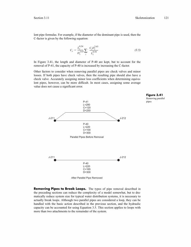
Section 3.11 Skeletonization 121
lent pipe formulas. For example, if the diameter of the dominant pipe is used, then the C-factor is given by the following equation:
CrLr0.54
Dr2.63
------------CiDi
2.63
Li0.54
------------------i
= (3.5)
In Figure 3.41, the length and diameter of P-40 are kept, but to account for the removal of P-41, the capacity of P-40 is increased by increasing the C-factor.
Other factors to consider when removing parallel pipes are check valves and minor losses. If both pipes have check valves, then the resulting pipe should also have a check valve. Accurately assigning minor loss coefficients when determining equiva-lent pipes, however, can be more difficult. In most cases, assigning some average value does not cause a significant error.
Figure 3.41Removing parallel pipes
Removing Pipes to Break Loops. The types of pipe removal described in the preceding sections can reduce the complexity of a model somewhat, but to dra-matically reduce system size for typical water distribution systems, it is necessary to actually break loops. Although two parallel pipes are considered a loop, they can be handled with the basic action described in the previous section, and the hydraulic capacity can be accounted for using Equation 3.5. This section applies to loops with more than two attachments to the remainder of the system.

122 Assembling a Model Chapter 3
Consider the three-pipe loop in Figure 3.42 made up of pipes P-31, P-32, and P-33. Removing any pipe in the loop can possibly result in a branch system that can be fur-ther skeletonized using the methods described previously. However, in contrast to the unique solutions that result from the pipe removal operations described in the preced-ing sections, the results of breaking this loop by removing a pipe are different depend-ing on which pipe is removed because the removal can have an impact on the carrying capacity of the rest of the system.
Figure 3.42Removing pipes in loop
Therefore, there needs to be a rule for determining which pipe should be removed first. Usually, it is best to remove the pipe with the least carrying capacity, which may be defined as the smallest or the pipe with the minimum value of the quantity
CD2.63
L0.54----------------- (3.6)
In Figure 3.42, pipe P-33 has the lowest carrying capacity so its removal should have the least adverse impact to the carrying capacity of the system.
It is important to note that removing the pipe with the least carrying capacity does not always do the least harm to the overall accuracy of the model. In some cases, a pipe with very little capacity may be very important in some scenario and may need to be kept in spite of its low carrying capacity.
Summary of Basic Pipe Removals. The results of the possible pipe removal actions can be summarized as shown in Table 3.2. The first three actions are fairly simple in that the system will end up with the correct flows and head loss. With the fourth removal action, however, some carrying capacity is lost and removing one pipe from a loop will give a different carrying capacity than removal of a different pipe.

Table 3.2 Summary of pipe removal actions
Action Effect on Node Loss of System Capacity
Remove branch pipe Removes node No
Remove pipe in series Removes node No
Remove pipe in parallel No nodes removed No
Remove pipe from loop No nodes removed Yes
Section 3.11 Skeletonization 123
Removing Nonpipe Elements. Removing link-type elements other than fully open pipes can be problematic, thus special rules must be developed for handling the skeletonization of other network elements including pumps, tanks, closed pipes, and valves.
A closed pipe or a pump that is not running has essentially already been skeletonized out of the system and any effort to skeletonize it is trivial. If the element may be open, however, then it should be treated as being open during the removal process.
Some other rules regarding the skeletonization of other network elements include the following:
• When loads are being aggregated from removed nodes, they cannot be passed through pumps, control valves, check valves, or closed valves.
• Pumps, control valves, and check valves in a branch can be trimmed and rep-resented as an outflow from the remaining upstream system.
• Pumps, control valves, and check valves can be removed from series, paral-lel, or looped systems only if their effect can be accounted for, which is usu-ally difficult.
• If there is a check valve on a pipe in series, the resulting pipe must also have the check valve.
• Tanks are usually too important to be removed during skeletonization and no pipes connected to tanks should be removed.
Complex Skeletonization. Skeletonizing a real system involves applying the basic removal actions in a sequence. In general, it is best to perform the skeletonizing actions in the order given in Table 3.2. First, remove all dead-ends or branch pipes, then remove series pipes, then combine parallel pipes, and finally, remove loops. After each action, it is necessary to review the network because the previous action may have created a dead-end or a parallel pipe that did not exist previously.
Figure 3.43, which shows a network being reduced, illustrates these actions. The net-work looks like a dead-end branch and if one were doing the skeletonization manu-ally, a modeler would simply add together the demands and place them on node J-10. However, it is difficult for a computer to recognize that this is a branch, and it must first eliminate series pipes and loops to identify the branch.
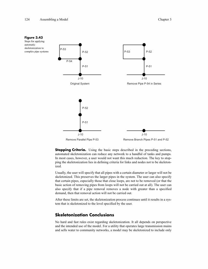
124 Assembling a Model Chapter 3
Figure 3.43Steps for applying automaticskeletonization to complex pipe systems
P-53
P-54
P-52
P-51
J-10
Original System
P-53 P-52
P-51
J-10
Remove Pipe P-54 in Series
P-52
P-51
J-10
Remove Parallel Pipe P-53
J-10
Remove Branch Pipes P-51 and P-52
Stopping Criteria. Using the basic steps described in the preceding sections, automated skeletonization can reduce any network to a handful of tanks and pumps. In most cases, however, a user would not want this much reduction. The key to stop-ping the skeletonization lies in defining criteria for links and nodes not to be skeleton-ized.
Usually, the user will specify that all pipes with a certain diameter or larger will not be skeletonized. This preserves the larger pipes in the system. The user can also specify that certain pipes, especially those that close loops, are not to be removed (or that the basic action of removing pipes from loops will not be carried out at all). The user can also specify that if a pipe removal removes a node with greater than a specified demand, then that removal action will not be carried out.
After these limits are set, the skeletonization process continues until it results in a sys-tem that is skeletonized to the level specified by the user.
Skeletonization Conclusions
No hard and fast rules exist regarding skeletonization. It all depends on perspective and the intended use of the model. For a utility that operates large transmission mains and sells water to community networks, a model may be skeletonized to include only

Section 3.12 Model Maintenance 125
the source and large-diameter pipes. For a community that receives water from that utility, the opposite may be true. Although most planning and analysis activities can be performed successfully with a moderately skeletonized model, local fire flow eval-uations and water quality analyses call for little to no skeletonization.
3.12 MODEL MAINTENANCEOnce a water distribution model is constructed and calibrated, it can be modified to simulate and predict system behavior under a range of conditions. The model repre-sents a significant investment on the part of the utility, and that investment should be maximized by carefully maintaining the model for use well into the future.
Good record-keeping that documents model runs and history is necessary to ensure that the model is used correctly by others or at a later date, and that time is not wasted in deciphering and reconstructing what was done previously. There should be notes in the model files or paper records indicating the state of the system in the various model versions. These explanations will help subsequent users determine the best model run to use as a starting point in future analyses.
Although the initial calibrated model reflects conditions in the current system, the model is frequently used to test future conditions and alternative piping systems. The scenario manager features in modeling software (see page 111) enable the user to maintain the original model while keeping track of numerous proposed changes to the system, some of which are never constructed. Eventually, a model file may contain many “proposed” facilities and demands that fall into the following categories:
• Installed
• Under design or construction
• To be installed later
• Never to be installed
The user needs to periodically update the model file so that installed piping is accu-rately distinguished from proposed facilities, and that facilities that will most likely never be installed are removed from the model. The modeler also needs to be in regu-lar contact with operations personnel to determine when new piping is placed into ser-vice. Note that there may be a substantial lag between the time that a pipe or other facility is placed into service, and the time that facility shows up in the system map or GIS.
Once a master plan or comprehensive planning study is completed, model use typi-cally becomes sporadic, though the model will still be used to respond to developer inquiries, address operations problems, and verify project designs. Each of these spe-cial studies involves creating and running additional scenarios. A single model even-tually becomes cluttered with extraneous data on alternatives not selected.
A good practice in addressing these special studies is to start from the existing model and create a new data file that will be used to study alternative plans. Once the project design is complete, the facilities and demands associated with the selected plan

126 Assembling a Model Chapter 3
should be placed into the main model file as future facilities and demands. The ver-sion of the model used for operational studies should not be updated until the facilities are actually placed into service.
REFERENCES
American Water Works Association (1996). “Ductile Iron Pipe and Fitting.” AWWA Manual M-41, Denver, Colorado.
Benjamin, M. M., Reiber, S. H., Ferguson, J. F., Vanderwerff, E. A., and Miller, M. W. (1990). Chemistry of
corrosion inhibitors in potable water. AWWARF, Denver, Colorado.
Caldwell, D. H., and Lawrence, W. B. (1953). “Water Softening and Conditioning Problems.” Industrial
Engineering Chemistry, 45(3), 535.
Eggener, C. L., and Polkowski, L. (1976). “Network Modeling and the Impact of Modeling Assumptions.
Journal of the American Water Works Association, 68(4), 189.
ESRI. (2001). “What is a GIS?” http://www.esri.com/library/gis/abtgis/what_gis.html.
Langelier, W. F. (1936). “The Analytical Control of Anti-Corrosion in Water Treatment.” Journal of the
American Water Works Association, 28(10), 1500.
Maddison, L. A., and Gagnon, G. A. (1999). “Evaluating Corrosion Control Strategies for a Pilot-Scale Distribution System.” Proceedings of the Water Quality Technology Conference, American Water
Works Association, Denver, Colorado.
McNeil, L. S., and Edwards, M. (2000). “Phosphate Inhibitors and Red Water in Stagnant Iron Pipes.” Journal of Environmental Engineering, ASCE, 126(12), 1096.
Merrill, D. T. and Sanks, R. L. (1978). Corrosion Control by Deposition of CaCO3 Films. AWWA, Denver,
Colorado.
Mullen, E. D., and Ritter, J. A. (1974). “Potable-Water Corrosion Control.” Journal of the American Water
Works Association, 66(8), 473.
Shamir, U. and Hamberg, D. (1988a). “Schematic Models for Distribution Systems Design I: Combination Concept.” Journal of Water Resources Planning and Management, ASCE, 114(2), 129.
Shamir, U. and Hamberg, D. (1988b). “Schematic Models for Distribution Systems Design II: Continuum
Approach.” Journal of Water Resources Planning and Management, ASCE, 114(2), 141.
Volk, C., Dundore, E., Schiermann, J., LeChevallier, M. (2000). “Practical Evaluation of Iron Corrosion
Control in a Drinking Water Distribution System.” Water Research, 34(6), 1967.
Walski, T. M. (1999). “Importance and Accuracy of Node Elevation Data.” Essential Hydraulics and
Hydrology, Haestad Press, Waterbury, Connecticut.
Walski, T. M. (2000). “Hydraulic Design of Water Distribution Storage Tanks.” Water Distribution System
Handbook, Mays L. W., ed., McGraw Hill, New York, New York.

Discussion Topics and Problems 127
DISCUSSION TOPICS AND PROBLEMS
Read the chapter and complete the problems. Submit your work to Haestad Methods and earn up to 11.0 CEUs. See Continuing Education Units on page xxix for more information, or visit www.haestad.com/awdm-ceus/.
3.1 Manually find the flow rate through the system shown in the figure and compute the pressure at node J-1. Also, find the suction and discharge pressures of the pump if it is at an elevation of 115 ft. Use the Hazen-Williams equation to compute friction losses. Assume hP is in ft and Q is in cfs.
R - A
R-B
J-1
Elev = 150 ft
Pipe 3:
L=1,000 ft
D=12 in.
C=120
Pipe 2:
L=2,200 ft
D=12 in.
C=120
Pipe 1:
L=220 ft
D=16 in.
C=120
h = 225P-10Q
1.50
125 ft
300 ft

128 Assembling a Model Chapter 3
3.2 Manually find the flow in each pipeline and the pressure at node J-1 for the system shown in the fig-ure. Assume that hP is in m and Q is in m3/s and note the demand at junction J-1 of 21.2 l/s. Use the Hazen-Williams equation to compute friction losses.
Hint: Express the flow in Pipe 3 in terms of the flow in Pipe 1 or Pipe 2.
J-1
Elev = 45.7 m
Pipe 3:
L=304.8 m
D=305 mm
C=120
Pipe 2:
L=670.6 m
D=305 mm
C=120
Pipe 1:
L=67.1 m
D=406 mm
C=120
h = 68.58P -639.66Q1.50
38.1 m
91.4 m
Q = 21.2 l/s
R - B
R - A
3.3 English Units: Manually find the discharge through each pipeline and the pressure at each junction node of the rural water system shown in the figure. Physical data for this system are given in the tables that follow. Fill in the tables at the end of the problem.
P-1
J-1
J-3
J-2
J-7
J-6J-5
J-4
J-11J-12
J-8 J-9
J-10
P-2
P-6P-4
P-3
P-5
P-8
P-7
P-9
P-12
P-11 P-10
(Not To Scale)
R -1
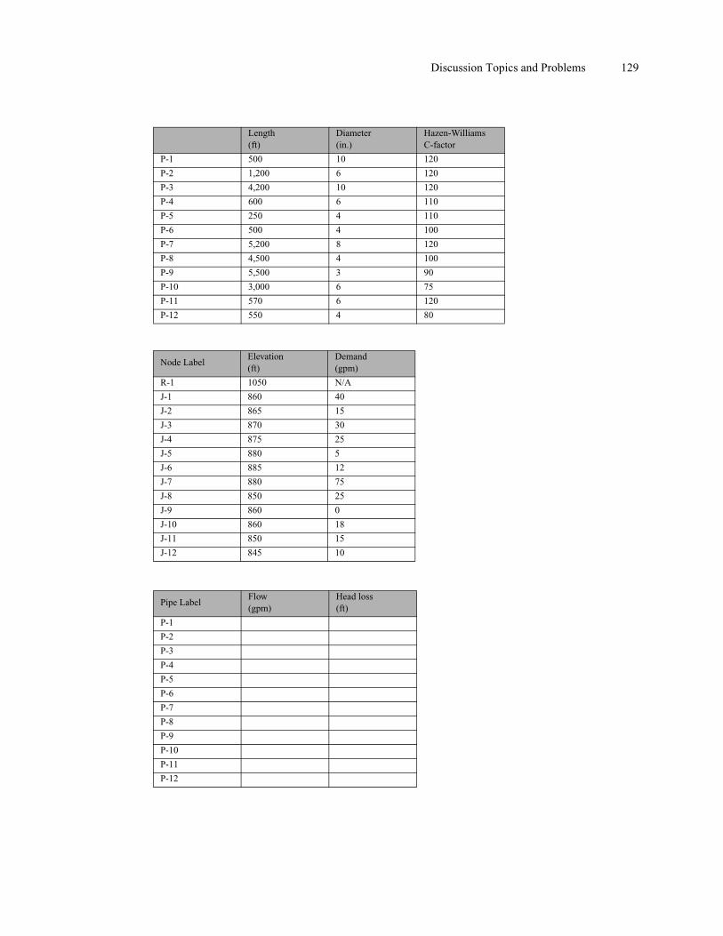
Pipe LabelLength(ft)
Diameter(in.)
Hazen-WilliamsC-factor
P-1 500 10 120
P-2 1,200 6 120
P-3 4,200 10 120
P-4 600 6 110
P-5 250 4 110
P-6 500 4 100
P-7 5,200 8 120
P-8 4,500 4 100
P-9 5,500 3 90
P-10 3,000 6 75
P-11 570 6 120
P-12 550 4 80
Node LabelElevation(ft)
Demand(gpm)
R-1 1050 N/A
J-1 860 40
J-2 865 15
J-3 870 30
J-4 875 25
J-5 880 5
J-6 885 12
J-7 880 75
J-8 850 25
J-9 860 0
J-10 860 18
J-11 850 15
J-12 845 10
Pipe LabelFlow(gpm)
Head loss(ft)
P-1
P-2
P-3
P-4
P-5
P-6
P-7
P-8
P-9
P-10
P-11
P-12
Discussion Topics and Problems 129

Node LabelHGL(ft)
Pressure(psi)
J-1
J-2
J-3
J-4
J-5
J-6
J-7
J-8
J-9
J-10
J-11
J-12
130 Assembling a Model Chapter 3
SI Units: Manually find the discharge through each pipeline and the pressure at each junction node of the rural water system shown in the figure. Physical data for this system are given in the tables that follow. Fill in the tables at the end of the problem.
Pipe LabelLength(m)
Diameter(mm)
Hazen-WilliamsC-factor
P-1 152.4 254 120
P-2 365.8 152 120
P-3 1,280.2 254 120
P-4 182.9 152 110
P-5 76.2 102 110
P-6 152.5 102 100
P-7 1,585.0 203 120
P-8 1,371.6 102 100
P-9 1,676.4 76 90
P-10 914.4 152 75
P-11 173.7 152 120
P-12 167.6 102 80

Node LabelElevation(m)
Demand(l/s)
R-1 320.0 N/A
J-1 262.1 2.5
J-2 263.7 0.9
J-3 265.2 1.9
J-4 266.7 1.6
J-5 268.2 0.3
J-6 269.7 0.8
J-7 268.2 4.7
J-8 259.1 1.6
J-9 262.1 0
J-10 262.1 1.1
J-11 259.1 0.9
J-12 257.6 0.6
Pipe LabelFlow(l/s)
Head loss(m)
P-1
P-2
P-3
P-4
P-5
P-6
P-7
P-8
P-9
P-10
P-11
P-12
Node LabelHGL(m)
Pressure(kPa)
J-1
J-2
J-3
J-4
J-5
J-6
J-7
J-8
J-9
J-10
J-11
J-12
Discussion Topics and Problems 131
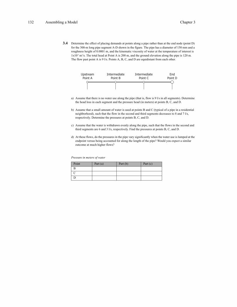
132 Assembling a Model Chapter 3
3.4 Determine the effect of placing demands at points along a pipe rather than at the end node (point D) for the 300-m long pipe segment A-D shown in the figure. The pipe has a diameter of 150 mm and a roughness height of 0.0001 m, and the kinematic viscosity of water at the temperature of interest is 1x10⁻⁶ m2/s. The total head at Point A is 200 m, and the ground elevation along the pipe is 120 m. The flow past point A is 9 l/s. Points A, B, C, and D are equidistant from each other.
UpstreamPoint A
IntermediatePoint B
IntermediatePoint C
EndPoint D
a) Assume that there is no water use along the pipe (that is, flow is 9 l/s in all segments). Determine the head loss in each segment and the pressure head (in meters) at points B, C, and D.
b) Assume that a small amount of water is used at points B and C (typical of a pipe in a residential neighborhood), such that the flow in the second and third segments decreases to 8 and 7 l/s, respectively. Determine the pressures at points B, C, and D.
c) Assume that the water is withdrawn evenly along the pipe, such that the flows in the second and third segments are 6 and 3 l/s, respectively. Find the pressures at points B, C, and D.
d) At these flows, do the pressures in the pipe vary significantly when the water use is lumped at the endpoint versus being accounted for along the length of the pipe? Would you expect a similar outcome at much higher flows?
Pressure in meters of water
Point Part (a) Part (b) Part (c)
B
C
D