Embed Size (px)
Citation preview

AD-A275 569
PL.TR-92-223i
Advanced Spectral Modeling Development
MG. DTICS.A. Cough ELECTERlD. Worsham JAN 2 6 1994
i ii i J.L. AbneetW.O. Gallery
Atmospheric and Environmental Reseawch Inc840 Memorial Drive(Cmbrldge, MA 02139
14 September 1992
Thal Report14 Juy 1989-14 July 1992
Approved for Public Release; distribution unlimited ,
PHILLIPS LABORATORYDirectorate of GeophysicsAIR FORCE MATERIEL COMMANDHANSCOM AIR FORCE BASE, MA 01731-3010
94-0228794 1 Ž5 070 1g llll

BestAvailable
Copy

•-L =z'ii-L'A • hla k~en reviewed and is approved for publication",
. te
C .IL• _,, Ar 5I•ON' . - ~ WILLUAM A.M. BLUMBERGBranch Chief
- - .|
ROOER A. VAN TASSEL 7Division-Directo
(its In kg 6,ziLvejiewed-b, the ESCPublic Affairs Office (PA) and is'relesable taj.eSlatiorml Te.ic Ijif0mation-SeMrvic (NTIS).
!Quaied mqlus.mt• may obtain addwitonal copies furomthe Defense Technical Information Center(DTIC). All others M. apply to th_ Nationo TehnicalInformation Service NTIS). -
if your Wdran has changed, or if you wish to be refidved from the mailing list, or if ,•itreswe-isno longer employed by your organization, please notify PLTSI, 29 Randolph RoV411.n. AFB; MA. 01731-3010. This-will assist us in maintaining a :urrent milling liHt
Do not retnw topieof this report. unless- ce-ftcfa- obligations or-notices otr a specrficdcfcument requires that it be returned. -
Bt•STAVAAILABLE'COPY

ftAI hufI IU. for 6i calleoitio of I I oisio essomd 10 , M I bow per -mapi ofta d aro - -mvvewng .inudmn sanmiamg uaammS desm asr. p magsa11 1 1 ~aamsusd. mpieftainpla Min muwg collaciomofiI Seaunood camouff - " das htimomues essa mry oaor upon of das adgcmua of wdofasa.
iaohhg~~~aima or ~oh ~ wd aWuhit-Huqa.Ihm Sa~ivior.I' DIcmu hibaw ido OPW~tiftm .ini bwM. 121 ISkn Do~avin s, ka4wy. Sal: 12W. Adunps. VA22215 W 01w wffof Mumpomi bigt. usmo mowdabmiuProject(070t.0IU) WuhaqeamDC 21511
1. ~~ A0IYUEOL P"bwk .ORT DATE & REPORT TYPE ANM DATE S COVERED
__~(Lm 1* 14 September 1992 Final (14 July 1989 - 14 July 1992)
Z TITE AND SUBTITLE 5. FUNDING NMBERSAdvanced Spectral Modeling Development PE 62101F
PR 7670 TAO09 WU BG
AUTHOR(S) Cnrc 688-- 5R. G. Isaacs R. D. Worsham W.Q. GalleryCotatF92--C0 0S. A. Clough J. L. Moncet
7. PERFORMING ORGANIZATION NAMES(S) AND ADDRESS(ES) S. PERORMING ORGANIZATION REPORTNUMBERS
Atmospheric and Environmental Research, Inc.840 Memorial DriveCambridge, MA 02139
9. SPONSORING / MONITORING AGENCY NAMES(S) AND ADDRESS(ES) 10. SPONSORING/IMONITORING AGENCYREPORT NUBE
Phillips Laboratory PL-TR-92-223 1H9anscom 3 Rd 1 731-3010
Contract Manager: Gail Anderson/GPOS _________
11. SUPPLEMENTARY NOTES
12&. DISTRIBUTION / AVAILADIUTY STATEMENT 12b DISTRIUTION CODEApproved for public release;Distribution unlimited
13 ABSTRACT (Aftxh~imn 200 waft)
This report describes the results of a basic research program to develop advanced spectralmodeling techniques to treat a variety of current topics in spectroscopy and radiative transferrelevant to the modeling of atmospheric transmission and radiance fields. These includeoptimizing multiple scattering, surface properties, line coupling, line shapes, interferometricinstrument function, and model validation. The overall goal of this research was the improvementof transmittance/radiance simulation modeling physics through continual model validation ofresults. Results of this study will enhance the capability to model atmospheric transmission andemission in support of DoD and other users.
The report is divided into sections based on model physics areas which were investigated inthe course of the contract. This work was done in support of the Advanced Spectral Modelingeffort conducted by the Phillips Laboratory, Optical Physics Division.
14. SUBJIECT TERMS 15. NUMBER OF PAGESAtmospheric transmission Spectral algorithm development 8Radiative transfer Spectroscopy _________
1& PRICE CODE
17. SECURITY CLASSiFICATION 1S. SECURITY CLASSIFICATION I19. SECURITY CLASSIFICATION 20. UMITATION OF ABSTRACTOF REPORT OF THIS PAGE OF ABSTRACT
Unclassified Unclassified Unclassified SARNSN 7540-01-2905M0 Stanard Form 296 (rev 2-89)
P~ascdbd by ANSI Std. Z39-19

TABLE OF CONTENTS
eIa.1. Introduction ........................................ 1
2 . A pproach ................................................................................. 2
3. Cross Section Data/Lorentz Capability ............................................. 2
4. Atmospheric Multiple Scattering ..................................................... 5
4.1 Large Solar Zenith Angle Scattering ........................................ 54.2 "Exact" Multiple Scattering .................................................. 10
5. Heating Rates and Fluxes ............................................................ 12
6. Scattering Properties of Precipitation ............................................... 17
7. Surface Properties ...................................................................... 19
7.1 Visible and Near IR Surface Reflection ................................... 197.2 Microwave Surface Emissivities ............................................. 22
8. Isotopic Ratios ......................................................................... 25
9. Instrument Function Enhancements ................................................ 27
9.1 Scanning Functions in the Spectral Domain ............................. 279.2 Scanning Functions in the Fourier Domain ............................. 28
9.2.1 Theory ...................................... 299.2.2 Examples .............................................................. 319.2.3 Implementation ...................................................... 33
9.3 Interpolation .................................................................... 33
10. Line Shape .............................................................................. 34
10.1 Line Shape for Carbon Dioxide ............................................ 3410.2 Line Coupling for Carbon Dioxide ........................................ 37
11. Collision Induced Bands ............................................................. 45
12. Spectral Model Enhancements ...................................................... 45
13. Advanced Spectral Model Validation ............................................... 48
13.1 Validation with Data from the High-resolution InterferometerSounder (HIS) ................................................................. 48
13.2 ITRA Microwave Validation ................................................. 58
m..

TABLE OF CONTENTS(continued)
13.3 High Altitude Modeling Support Activities ................................ 6513.3.1 M SX ................................................................... 6513.3.2 Celestial Occultation Experiment .................................. 6613.3.3 Earthlimb Experiments ............................................. 6813.3.4 MSX Contributions to Global Climate Monitoring ........... 69
14. Support for Annual Review Conference ........................................... 69
15. Conclusions .............................................................................. 72
16. R eferences ................................................................................ 72
Accesion For
NTIS CRA&I
DTIC TABEUlnannoun1cedJustificatiorn
By ...............................Distribution I
Availability Codes
Avail andj orDist Special
iv

LIST OF FIGURES
E~m
1 The contribution of CC14 (790 cm- 1), CFC 11 (850 cm- 1) and CFC 12(925 cm-!) to the transmittance of an atmospheric layer at 975 mb ............. 6
2 The transmittance of the same layer as Figure I except that the that thespectral cross section data have been convolved with a Lorentzian toaccount for the effect of atmospheric pressure broadening ...................... 6
3 M ultiple scattering "quick fix". ...................................................... 8
4 Multiple scattering "quick fix": comparison to DOM ............................ 9
5 Interface routine ....................................................................... 11
6 Limb layer radiance spectrum utilized for development of the improvedradiance algorithm. The units are equivalent brightness temperature .......... 14
7 Radiance error in equivalent brightnesm temperature due to treatment ofthe layer as isotherm al ................................................................ 15
8 Radiance error utilizing the improved radiance algorithm ........................ 15
9 Legendre polynomial coefficients of a Marshall-Palmer size distributionwith a rainfall rate of 5 mmh- 1 at four frequencies ................................ 18
10 Spectral albedos for different surface types. Curves are given for newsnow (@), old snow (A), a plowed field of clay loam (+), green plants(x), and a smooth ocean at solar zenith angles of 0* (0) and 550 (T) ........... 21
11 LOWTRAN radiance calculations with surface albedos in Figure 11 .......... 23
12 (a) Variation of 540 look-angle polarized emissivity (ev, e) with surfacemodel at frequencies of 1.2, 5.0, 10.6, 18.0, and 35.0 GHz. (Surfacemodels 1-6, Table 3) (b) Same as (a). (Surface models 7-12, Table 3.) ...... 26
13 The Five FTS Scanning Functions and Their Associated ApodizationFunctions Available in FFTSCAN .............................................. 30
14 (a) FASCODE Calculated Spectrum Smoothed by FFTSCAN Plus TheError In the Smoothed Spectrum from using: (b) FFTSCAN WithBoxcaring, and (c) the FASCODE3 Scanning Function ......................... 32
15 The chi function for carbon dioxide with Vo = 2 cm-1 . The solid line isfor halfwidth of 0.08 cm-1 (1 atm) and the dashed line is for a halfwidthof 0.008 cm -1 (0.1 atm ) . ......................................................... 36
v

LIST OF FIGURES (continued)
gm EM
16 The chi function for carbon dioxide with V. = 8 cm-1 . The solid line isfor halfwidth of 0.08 cm-1 (I atm) and the dashed line is for a halfwidthof 0.008 cm -1 (0. 1 atm ) ............................................................ 36
17 (a) Calculated limb transmittance spectrum with Vo = 2 cm-1;(b) Calculated limb transmittance spectrum with Vo = 8 cm-I ....... . . . . . . . . . 38
18 An ATMOS occultation transmittance spectrum. The tangent height is20.5 km . ............................................................................... 39
19 A calculation with Vo = 2 cm-I for the measurement conditions ofFigure 19 . ............................................................................. 39
20 Limb transmittance spectrum for the conditions of the ITRAintercomparison with a 30 km tangent height for Vo = 2 cm- ...... . . . . . . . . . . . . 40
21 Limb transmittance spectrum for the conditions of the ITRAintercomparison with a 30 km tangent height for Vo = 8 cm-I ...... . . . . . . . . . . . . 40
22 Effect of line coupling on the spectral residuals for the nadir HISobservation of 14 April 1986: a) no line coupling, b) line coupling withthe basis coupling coefficients, and c) basis coupling coefficientsmultiplied by a factor of 1.3 ........................................................ 42
23 Effect of line coupling on the spectral residuals for the zenith observationof 1 November 1988 with the HIS instrument: a) no line coupling, b)line coupling with the basis coupling coefficients, and c) basis couplingcoefficients multiplied by a factor of 1.3 .......................................... 43
24 Brightness temperature residuals associated with Figure 22 as a functionof brightness temperature ............................................................ 44
25 HIS equivalent brightness spectra from April 14, 1986: nadir view overocean from 19.6 km .................................................................. 52
26 The difference spectrum in equivalent brightness temperature between thespectrum of Figure 26 and a calculated spectrum using FASCODE withthe 1986 H1TRAN line parameters. An error of I K in the windowregion at 1000 cm-I corresponds to a 1.6% error in radiance ................... 52
27 The difference spectrum in equivalent brightness temperature between thespectrum of Figure 26 and a calculated spectrum using FASCODE withthe inclusion of the effects of line coupling and improved carbon dioxideline param eters ....................................................................... 54
vi

LIST OF FIGURES (continued)
28 The difference spectrum in equivalent brightness temperature between thespectrum of Figure 26 and a calculated spectrum using FASCODE. Theeffect of CC14 at 795 cm- 1, CFCI 1 at 850 cm-1 and CFC12 at 920 cm-1have been taken-into account in addition to the effects included inFigure 28 . ............................................................................. 54
29 The difference spectrum in equivalent brightness temperature between thespectrum of Figure 26 and a calculated spectrum using FASCODE. Theeffect of a thin cirrus cloud at 13 km has been included in addition to theeffects treated in Figures 28 and 29 ................................................ 55
30 Zenith radiance spectrum observed with the U. of Wisconsin HISinstrument at Denver, CO, 1 Nov. 1988, as part of the GAPEXcampaign. ............................................. 57
31 Radiance residuals between the observed spectral radiance of Figure 31and a FASCODE calculation with a radiosonde defined atmosphere ........... 57
32 Sources of Spectral Radiance as Seen by the Spirit III InterferometerViewing the Limb at a Tangent Height of 60 km. ................................ 67
33 Timeline for the stairstep maneuver for ELE-I .................................... 70
34 Experiment timeline, from park to park, for ELE- 1 showing theinstrument modes, the spacecraft maneuvers, and the orbital positions ........ 70
35 Timeline for the sawtooth vertical profile scan for ELE- 10 ...................... 71
vii

LIST OF TABLES
1 First Moment Quadrature Direction Cosine Values, Weights andRepresentative Flux Errors ............................................................ 16
2 Radiative Source Functions. Forms of Boundary, Ri(Pb), and
Atmospheric, S(p), Contributions to Sensor-incident Radiances, Ri(6) ........... 20
3 Surface Model Types and Modeling Approaches .................................... 24
4 Comparison of Computational Time and Accuracy Among Three ScanningFunction Options for the Sinc, Sinc2, and Triangle Scanning Functions ......... 33
5 Characteristics of the HIS Instrument for Flight of 14 April 1986 ................ 49
6 The Input Atmosphere for the Validations in FASCODE Format .................. 50
7 Abbreviated Input file for Atmospheric Layering Associated with ITRAMicrowave Comparison ................................................................ 59
8 Layer Specifications Resulting from the Input File of Table 7 ...................... 61
9 Earthlimb Experiment Plans ............................................................ 68
viii

1. INTRODUCTION
The Air Force Phillips Laboratory, Geophysics Directorate (PLJGP) has developedtwo extensively used radiative transfer codes: LOWTRAN (Kneizys et al., 1983) and
FASCODE (Clough et al., 1981 and Smith et al., 1978). The current implementations ofthese codes are LOWTRAN 7 and FASCOD3, respectively. FASCODE is a computercode for the accelerated line-by-line calculation of spectral transmittance and radianceapplicable from the microwave to the near ultraviolet (Clough et al., 1986). LOWTRAN isa computer code with a resolution of 20 cm-1 utilizing a one parameter band model. Thetwo codes share extensive common elements including the spherical refractive geometrycapability, the aerosol models, and the molecular continuum. For LOWTRAN 7 themolecular band model parameters have been obtained from FASCODE calculations usingthe 1986 HITRAN database (Rothman et al., 1987), significantly extending the
compatibility between the two codes. Some differences exist, primarily as a consequenceof the algorithms required to handle the molecular absorption. In particular, the multiplescattering is treated differently and capabilities such as non-local thermodynamic
equilibrium (NLTE) that are dependent on temperature cannot be implemented inLOWTRAN since it is a single parameter model.
As effective as these models are, the user community requires more accurateradiative transfer calculations for even more complex environments. These requirementsrelate to atmospheric state definition, long path surveillance, radiative transfer in cloudyenvironments and improved capabilities for highly disturbed environments. This reportdescribes the results of a program in advanced spectral modeling to address theseincreasingly stringent requirements. The approach taken in this program has been toimprove model physics with improvements quantified and assessed by model validation.AER scientists have worked closely with Geophysics Directorate counterparts whoprovided technical direction and prioritization of relevant topics explored.
Although, as described above, the AFGL line-by-line code already possesses manyof the attributes desired of a generally applicable transmittance/radiance simulation code, itlacks a number of desirable and potentially useful capabilities. These include the capabili-ties to: (a) accommodate the use of cross section data for transmittance calculations, (b)perform generalized multiple scattering calculations, (c) calculate both heating anddissociative fluxes, (d) provide radar and lidar backscatter coefficients, (e) incorporatesurface reflection and emissivity effects including those of surface polarization on

atmospheric radiance calculations, (f) extend NLTE capabilities, (g) modify the isotopic
ratio, and (h) perform Fourier transform/interferometer studies.
This report is subdivided into task specific subsections. The following section
describes our general approach to address these technical issues (Section 2). Subsequentsections provide descriptions of work performed to accommodate new physics.
2. APPROACH
Advanced spectral modeling techniques are required to treat a variety of currenttopics in spectroscopy and radiative transfer relevant to the modeling of atmospheric
transmission and radiance fields. As alluded to in the introductory section above, these
topics include optimizing multiple scattering, surface properties, line coupling, line shapes,interferometric instrument function, and model validation. While the topics are varied,
improvements in modeling these phenomena will enhance the integrated capability of
Phillips Laboratory atmospheric transmission and radiance computer codes to be applied insupport of DoD and other users. The approach which has been taken in this study has been
to improve the simulation modeling physics of specified submodel areas (with prioritization
guidance by the Phillips Laboratory) based on a process of continual model validation of
results. By comparison of model output results to data, the integrated effect of individualsubmodel improvements is assessed in a manner consistent with that experienced by the
user community. While appropriate data did not always exist to test improvements in
specific submodel areas, our overall goal was to validate enhancements with real data.
3. CROSS SECTION DATA/LORENTZ CAPABILITY
There are applications in radiative transfer for which it is not possible or not feasible
to perform exact calculations. An obvious case is the one for which spectral line
parameters are not available. Another situation arises in which the spectral density of
transitions is so high that, for efficiency, it may be desirable to replace the line-by-line
calculation with available cross section spectra without serious loss of accuracy. The initial
implementation of a module to incorporate the effects of absorption by heavy molecules
into the advanced spectral model was accomplished with the cross section data from the
1986 HITRAN database. File four of the 1986 AFGL line compilation (Rothman et al.,1987) includes seventeen spectral cross sections for eleven molecular species. These crosssection data from the 1986 HITRAN database were only available for a single temperature
2

and pressure and their application at other temperatures and pressures constituted an
approach that could involve unacceptable error.
The 1992 HITRAN database includes cross section data at more than a single tem-
perature for many of the heavy molecular species. The initial version of the cross section
module has been extensively enhanced to adapt the cross section data to the thermodynamicconditions of the atmospheric layer for which the molecular optical depths are required. The
treatment of the temperature dependence for the cross sections has been achieved by linearly
interpolating to the specified layer temperature. Cross section data are provided at a variety
of pressures, generally pressures substantially lower than atmospheric reference pressure
(1013 mb) appropriate to the lowest part of the atmosphere. While it is not feasible to
address the problem in which the cross section optical depths are required at pressures lower
than that for which the data is provided, the case in which the optical depths are required at
higher pressures can be addressed. Since many of the atmospheric effects of the heavymolecules occur at the lower altitudes it is desirable to have an approximate approach that
provides an improved result at the higher pressures. This has been accomplished by
assuming that the cross section data are coilisionally broadened and that the average collision
broadened halfwidth for all lines is 0.08 cm-I at 1013 mb. The temperature dependence of
this assumed halfwidth value has not been taken into account, a consideration for future
enhancements. The line shape for collisional broadening is the Lorentz shape. We takeadvantage of the fact that a Lorentzian of width aj convolved with a Lorentzian of width a
a12 results in a Lorentzian with width aX + a2. This result can be readily established by
considering the convolution in the Fourier domain. Utilizing the fact that the Fouriertransform of the Lorentzian is an exponential and that in the Fourier domain the convolution
operation is represented by a product, we obtain directly the result that the resulting functionis a Lorentzian since the product of two exponentials is itself an exponential.
In cases for which the available cross section data have been extrapolated to zero
pressure for application to stratospheric problems, the line shape appropriate to the data is
taken to be the Doppler shape. The same procedure as previously described is utilized toobtain cross sections at the specified pressure. Although in principal this procedure is not
rigorous in the sense of the convolution of Lorentzians, it is likely to be a reasonable
approximation since for most cases of interest the Doppler width will be considerably
narrower than the final Lorentz width. This result is a consequence of the fact that the
convolution of a narrow Doppler shape with a broad Lorentzian is a Lorentzian to good
3

approximation. In the limit of an infinitely narrow Doppler line, i.e. a 8 function, the
procedure becomes rigorous.
To implement the approximate method for correcting the data to higher pressures,
we first establish the mean halfwidth of the data as 0.08 * (Pc / Po) where Pc is the
pressure at which the data are provided and Po is 1013 mb. The value of 0.08 cm-1/atm is
chosen as representative of the molecular atmospheric pressure broadening coefficient. We
next calculate the collisional halfwidth for the atmospheric layer for which the optical
depths are required as 0.08 * (P1 / Po) where PI is the specified layer pressure. To correct
the cross section data to the layer pressure, the data are convolved with a Lorentzian of
width 0.08 * [ (PI / Po) - (PC / Po) ] in which it is required that this be a positive quantity.
A further constraint is imposed with respect to the sampling interval of the data: the
sampling interval is specified as a fourth of the mean layer halfwidth. If this sampling
interval is less than 10% greater than the sampling interval at which the cross section data
are provided no convolution is performed.
In working with Laurence Rothman at PLJGP on the format for the cross sections,
a determination wa. made that it would be advantageous to include in the header the
minimum and maximum value of the cross section value in the related spectral cross section
record. ' t an early stage of the calculation of the cross section contribution to each layer,
the maximum value of the cross section value is utilized in conjunction with the appropriate
column amount to determine whether the inclusion of a particular cross section set is
required. The decision is made relative to the value of the minimum optical depth parameter
(DPTMIN), an input parameter which prescribes the minimum optical depth contributions
to be included in the optical depth calculation for the current layer.
To expedite the inclusion of cross section contributions into the layer optical depthcalculations the following approach has been implemented: based on the sampling interval
for the cross sections as prescribed by the considerations discussed above, the cross
section contribution is added to the optical depths in the appropriate array RI, R2, R3 or
R4 using the four point Lagrange interpolation method. The choice of the appropriate arrayis determined as that array whose spectral sampling interval (DV) has the closest smallervalue to that of the cross section results. The incorporation of the cross section data into
the FASCODE calculations has utilized concepts and modules that are already available in
FASCODE. The largest task has been in interlinking the available modules and interfacing
the data files.
4

Vertical profiles of mixing ratio (Jan., Apr., Jul., Oct.) at latitude 28N (chosen asrepresentative of a global average) were provided from the 'AER 2d chemistry model' forthe following trace gases for consideration for incorporation into the XAMNTS module ofFASCODE: CC14, CFC 13, CFC13F3, CIONO3, N20 5, H0 2NO2, HNO3. An exampleof the effect of the convolution method is given in Figures 1 and 2. Figure 1 provides the
contribution of 3 cross section molecules to the transmittance for the lowest layer in amultilayer nadir case. In Figure 2 we have the result for the same case as Figure I exceptthat the convolution has been performed to provide a result consistent with the pressure ofthe layer. The spectra are attributable to CC14 at 790 cm-1, CFC 1I at 850 cr 1I and CFC 12
at 925 cm-1. The pressures at which the cross section data are provided &re 0.453 mb forCC1t, 0.0933 mb for CFCl 1, and 0.266 mb for CFC 12. The pressure of the atmosphericlayer is 975 mb. Results of validations with HIS observations which include the effects ofthese heavy molecules have been generally favorable.
4. ATMOSPHERIC MULTIPLE SCATTERING
Preliminary studies of the implementation of the multiple scattering option in the
AFGL spectral modeling codes (LOWTRAN, MODTRAN) has suggested some
deficiencies in the current treatment. The current PLjGP band model for LOWTRAN treatsmultiple scattering through the use of a two-stream approximation to the radiative transferequation, incorporating gaseous absorption with an exponential sum or k-distributiontechnique (Isaacs et al., 1987). This treatment is perhaps the most efficient one possible tohandle multiple scattering, but it does break down in some regimes.
First, it was recognized that the approach as implemented did not explicitly treatcases in which earth sphericity was a factor, i.e. when the solar zenith angle cosineapproached and exceeded 900. Secondly, it was desired to provide an alternate highaccuracy approach which directly incorporated the capability of a multistream multiplescattering model. Both these enhancements are described below.
4.1 Large Solar Zenith Angle Scattering
The multiple scattering approximation implemented in LOWTRAN and MODTRAN
is based on the assumption of plane parallelism. The computational manifestation of thisassumption is the appearance of the secant or inverse cosine air mass factor which is used
5

WAVELENGTH (MICROMETER)1 1.o ! .5 13;.o0 11.5 11•.0
1.000 1.000
z2 0.999 0.999i
z
0.99a 0.998
0.99------- - 0.997750 775 800 825 850 875 900 925 050
WAVENUMBER (CM-I)t17A1I g21..1 l fl j 11 6 .44.f1
Figure 1. The contribution of CC14 (790 cm'1 ), CFCII (850 cm"1) and CFCI2 (925 cm"]) tothe transmittance of an atmospheric layer at 975 mob.
WAVELENGTH (MICROMETER)1 ;,o 1 J.5. .!.5 11.0
1.000 1.000
U)
0.998 0.998
0.991. . . . . . 0.997750 775 800 825 850 875 900 925 950
WAVENUMBER (CM-i)
Figure 2. The transmittance of the same layer as Figure)I except that the that the spectralcross section data have been convolved with a lorentzian to account for the effect
of atmospheric pressure broadening.
6

to convert between vertical optical path quantities and slant path optical properties. This
assumption is used extensively in the calculation of the two stream equations which provide
the approximation of scattered intensities for the multiple scattering source function.
A simple approach to treating the spherical geometry of high zenith angle, i.e. lowsun cases, with respect to multiple scattering of solar radiation, recognizes that the primary
solar scattering source function can be defined by evaluating the attenuation of the directsolar beam over the exact refracted path. The primary solar scattering source function is
then calculated exactly as it is in the single scattering option, by replacing the secant of the
SZA (solar zenith angle) as the air mass factor with the ratio of the actual refracted pathoptical thickness to the vertical path optical thickness for each layer. This eliminates theartificial singularity at the horizon (solar zenith angle of 90 degrees) and produces a realistic
source function which degrades monotonically to zero.
Physically, the multiple scattering calculation uses the exact primary source functionevaluated for the spherical atmosphere, but then assumes plane parallelism for thecalculation of the multiple scattered contributions to path radiance. We call this the locally
plane parallel approximation.
The approach we have adopted to implementing this enhancement is the following:
- Working with GL personnel, we identified the refracted path opticalthickness for the solar path and the vertical path optical thickness corresponding to this pathfor each layer. The ratio of the former to the latter was defined as the air mass factor.
- The reciprocal of the air mass factor thus derived was defined as theeffective solar zenith angle cosine for the multiple scattering approximation. This quantity
has the following properties: (a) no singularity at 90 degrees, (b) it is not symmetric about
90 degrees, (c) it decreases monotonically but never reaches zero.
- Radiances were calculated as a function of SZA for a downward lookingpath originating at 30 km at 10,000 cm-I (assuming zero surface albedo). These are shownin Figure 3.
7

-8I
C
q" old.o. -9:new
11. . , , ,
86 88 90 92 94 96angle
Figure 3. Multiple scattering "quick fi'x
In the previous plane parallel (pp) formalism there was a singularity at a SZA of 90
degrees. A GL fix [denoted old(89)] constrained this angle so that it was symmetric about
90 degrees with the SZA fixed at 89 degrees for angles from 89 up to 91 degrees and so
that the airmass factor [here defined as l/cos (SZA)J was positive definite for angles greaterthan 91 degrees.
It is seen that the pp approach blows up at 90 degrees as expected and the radianceis underestimated due to using the reciprocal of the cosine at large angles which under-estimates the primary source function. The GL fix [old(89)] overestimates the radiance dueto fixing the SZA at 89 degrees. The new approach is well behaved.
Calculations were also done to compare the results of this treatment for large zenithangles within the approximations used in MODTRAN and LOWTRAN to exact resultsfrom application of the discrete ordinate method (DOM). This comparison was facilitatedby the LOWTRAN/DOM interface described in the following section (Section 4.2).Results of this comparison are shown in Figure 4. These include: (a) the new treatmentand DOM results using (b) two and (c) eight streams, respectively. The figure illustrates
that the new treatment is consistent with the eight stream DOM results for all solar zenith
8

0.0010!
0.0008
0 0.0006UC
* 0.0004 _- DOM (2)E. -.-- DOM (8)
0.0002 - LOWTRAN
0.0000 .1 -•0 20 40 60 80 100
Angl
Figure 4. Multiple scattering "quick fix": comparison to DOM.
angles. It can be seen that over the range from over head sun to sun at the horizon(SZA=0, 90), the LOWTRAN approximation (although a two stream approach) gives a
better fit to the eight stream DOM results than to the DOM two stream. This is because the
DOM and LOWTRAN two stream approximations are inherently quite different. In fact,
the LOWTRAN two stream solution (a hybrid modified delta-Eddington approximation)
was selected specifically for its better fit to exact multiple scattering results.
The same improvements suggested here for LOWTRAN can be applied to the
moderate resolution model MODTRAN.
In modifying LOWTRAN 7 to correctly calculate the large solar zenith case, one
goal was to minimize the changes necessary so that any forth-coming errata would be as
simple as possible. With this in mind, all changes to LOWTRAN were constrained to the
subroutine FLXADD. In this routine the variable CSZEN is redefined to be the ratio of the
refracted path optical thickness to the vertical path optical thickness. This required the
addition of twenty-three lines of code to FLXADD.
9

Other changes which should be considered, but which were not implemented are:
1) remove the GL fix in routine LWTRN7 which constrains CSZEN to 89
degrees (not currently a problem since CSZEN is reset in FLXADD to correct
value).
2) remove references to CSZEN in routine SSGEO since this calculation of
CSZEN is no longer necessary.
An updated version of FLXADD has been made available to PUGP.
4.2 "Exact" Multiple Scattering
A particular deficiency of the multiple scattering approximation is the two stream
approach. At the time of its development an accuracy of 20% in radiance was deemed
acceptable. Subsequently, user requirements have driven the need for more accurate scat-
tered radiance fields, particularly for the calculation of backgrounds. The most dramaticimprovement of multiple scattering accuracy would come about by changing from a two-
stream approximation to a multiple stream scattering model. There are two approaches to
the multiple stream multiple scattering problem that have significant and complimentary
advantages. The adding-doubling method is highly accurate and is fast for applications in
which the spectral radiance at a specific atmospheric level is required. For applications in
which the radiative transfer result is required for the full atmosphere, net fluxes and heat-
ing/cooling rates, and for which the number of spectral points is not extremely large,
LOWTRAN resolution, the discrete ordinate method (DOM) offers some distinct
advantages.
An efficient, accurate, and well tested DOM code has recently become available
(Stamnes and Conklin, 1984). The number of streams can be selected by the user to be
anywhere from 2 to 64, depending on the problem the user is interested in. In the two-
stream mode the code would behave as the one currently in LOWTRAN, although it would
be a bit quicker. The accuracy increases markedly as the number of streams increases, but
so does the computation time. Four streams is easily a factor of 2 or 3 more accurate than
two streams, while eight streams is easily an order of magnitude more accurate. Further-
more, the need for a diffusivity factor disappears when a multi-stream approach is used,
removing another approximation. The multiple stream code would be particularly helpful
10

for solar or lidar cases, and is essential if one wishes to expand LOWTRAN's capabilitiesto include dusty and cloudy atmospheres.
The approach to provide an "exact" multiple scattering capability with LOWTRANwhich introduced minimal program impacts was to link the LOWTRAN and DOM codes.To accomplish the required connectivity between the LOWTRAN atmospheric profileoptical properties and the DOM code, an interface routine is provided. This is illustrated inFigure 5.
LOWTRAN was modified by adding approximately sixty lines of code, consistingmostly of write statements into the body of routines LWTRN7 and TRANS. This modifiedversion of LOWTRAN produces an additional output file which is read in by the DOMinterface code DOMLOW. The following information is provided to DOMLOW fromLOWTRAN for each frequency:
frequency interval
rsolar intensitysolar zenith anglelook angle
LCWTRMsurface albedosurface temperature
layerasymnetry factorair mass factortemperaturefor each Icsingle scatter albedooptical thicimess
Figure 5. Interface routine.
11

"* frequency, wavelength and bounds for current frequency interval."* azimiuth angle, solar intensity at top of atmosphere, solar zenith angle at surface,
cosine of theta (look angle), surface albedo, surface temperature and number oflayers.
"* profile of asymmetry factors at every layer, the effective air mass factor (ratio ofrefracted path optical thickness to vertical path optical thickness) and the layeredge temperatures.
"* profiles of single scattering albedo and optical thickness for each layer and valueof k.
User selection of atmospheric model follows from LOWTRAN. The interface routinereads in the output file described above, and calls the DOM subroutine.
DOMLOW has been made available to PL/GP.
5. HEATING RATES AND FLUXES
The capabilities in the present PLJGP line-by-line model extend to providing userswith two fundamental radiative properties of atmospheric paths, namely transmittance andradiance. Another derived quantity of interest to atmospheric modelers is the flux profile,F, associated with atmospheric heating. The upward and downward flux profiles aredefined as:
while the net flux is given simply by:
F(v,r)=JfJ(vrp)dy =F4 -P
here I is the frequency dependent, azimuthally averaged radiance field, T is the opticalthickness which can be related to atmospheric level, and g± is the direction cosine. Heatingrates are obtained by differentiating the net flux with respect to an appropriate pathparameter such as height, i.e. the heating, h(z), would be proportional to:
h(z)adF(v) ddr dz
12

The development of the capability to obtain fluxes and heating rates for advanced spectral
modeling has been performed in conjunction with support from DOE. The effort has
involved three aspects: (1) the development of an improved algorithm to calculate radiancesfor a vertically inhomogeneous layer, (2) modifications to the line-by-line radiative transfermodel (FASCODE) to provide the necessary intermediate radiance results including anappropriate spectral averaging method; and (3) an algorithm to compute the fluxes and
heating rates from the intermediate radiances. The implementation and validation of the
improved radiance algorithm was accomplished through the support of the current contract.
An important problem in atmospheric radiative transfer is the treatment of vertical
inhomogeneity, particularly with respect to the treatment of the variation of the Planck
function in the inhomogeneous layer. This is a particularly important issue in the
calculation of cooling/heating rates which involves the calculation of the flux divergence. A
method has been developed which has gained general acceptance in the field of radiativetransfer to address the problem of the vertical inhomogeneity of the temperature field. It is
called the 'linear in tau method' from the assumption that the Planck function varies linearly
from a value appropriate to the level boundary in the direction of the radiation (optically
thick limit) to one appropriate to an average for the layer (optically thin limit). This
approach was considered by us to have had a number of limitations: (1) the associated
algorithm is computationally expensive; (2) the result involves a division by the opticaldepth requiring the definition of a strong and weak regime; (3) there is no mechanism to
account for the variation of the optical depth in the path (i.e. the exponential atmosphere);
and (4) it was not initially obvious how to accommodate a value of the Planck function in
the thin limit that deviated from the average Planck function for the layer. An algorithm hasbeen developed which is designed to avoid some of these problems and has the advantage
of being computationally fast.
The algorithm for the radiance from a layer, R, in which the Planck function varies
along the optical path in the layer, is given in our approximation by the relation:
R = [i. (aT . I+ r- I-rT)
where B is the Planck function appropriate to the optically thin limit, B is the Planckfunction associated with the layer boundary in the direction of the radiance, 'r is the optical
depth of the layer, T is the associated transmittance, and all quantities are to be taken at the
13

monochromatic frequency of the calculation. The parameter a in this Padd approximationhas been obtained empirically from studying a number of zenith, nadir and limb simula-tions. A value for the constant a of 0.20 provides a significantly improved result over an
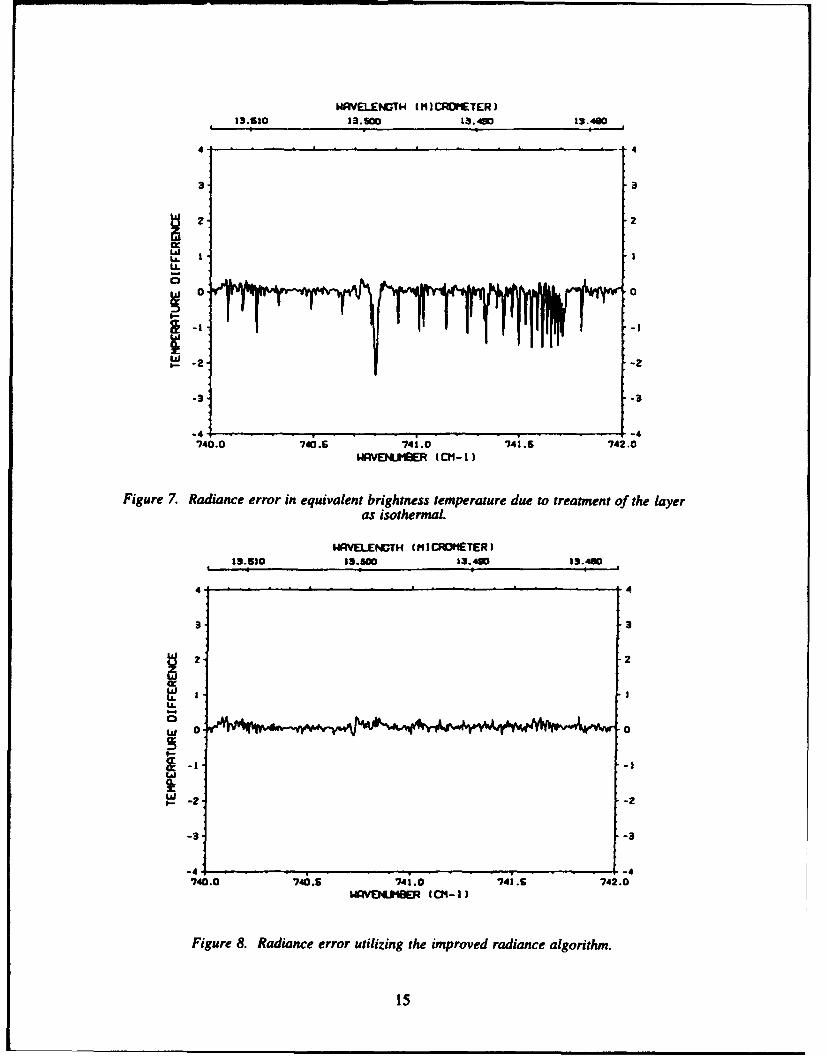
algorithm that does not take into account the vertical inhomogeneity of the temperaturefield. Figure 6 indicates the spectral radiance in equivalent brightness temperature in arepresentative spectral region from 740 cm-I to 742 cm-I for a simulated limb calculation.The reference calculation has been obtained by dividing the limb layer into five sub-layersand utilizing the new algorithm in the calculation. Figure 7 demonstrates the error obtained
when the limb layer is treated as a single isothermal layer at the path weighted temperature
of the layer. Figure 8 demonstrates the error when the limb layer is treated as a single layer
and the new algorithm for radiance is utilized. It should be emphasized that in the optically
thick limit the new algorithm provides correct radiance values at the layer boundaries. Thisis essential to ensure that in this limit the net flux at the boundaries is zero, resulting in no
net heating or cooling. The algorithm for calculating fluxes has been made available atPUGP on file FLUXF/UN=ISAACS. We are indebted to Gail Anderson and Frank
WAVELENOTH (MIICROMETER)13.510 13.100 13.490 13.460
IS I 1 I i 4
140-
120-
1001
74o.0 740.5 '71.0 "41.5 "i.o
WAVENUBER C'M-I1)
Figure 6. Limb layer radiance spectrum utilized for development of the improved radiancealgorithm. The units are equivalent brightness temperature.
14
WAVELENGTH (1 ]CRO1ETER)
13.510 13.500 13.4M0 13.4w0
4- 4
3 3
12.21° °L&
S00
--2
-3 -
-4 -4740.0 740. 741i.0 741.5 742.0
WPAVEJ4JHER ICM1-1)
Figure 7. Radiance error in equivalent brightness temperature due to treatment of the layeras isothermal.
Wi.AVELENGTH (MICROHETER)15s10 25.5M 13.4D 13.4w0
4 . . . . . .. .. 4
3 3
.2
IL.
00 -0
d -2 -1 -1
w - -z
-3 -3
-4 ' . . .. .. ...-,4
i4 0.0 746.r. 74 1.0 4 ,, .G 7424.0WgIVE.UIBER (C0-1)
Figure 8. Radiance error utilizing the improved radiance algorithm.
15

Kneizys for discussions leading to an appropriate treatment in the optically thin limit. In
the final analysis our concerns with the linear in tau method may have been greater than
appropriate and with judicious coding this approach may ultimately prove preferable.
The strategy implemented for computing fluxes is as follows: (1) the line-by-line
calculation of optical depths for the nadir is performed and the results retained for sub-
sequent utilization; (2) the radiances are calculated using these spectral optical depths multi-
plied by the reciprocal of the direction cosine associated with the angle for which the
radiance is required; (3) the monochromatic radiances are spectrally degraded at each layer
to reduce storage and data handling requirements; and (4) the fluxes are obtained from the
upwelling and downwelling degraded spectral radiances to provide the up- and down-
welling fluxes. New radiance algorithms are provided for this calculation due to the neces-
sity to merge from the top of the atmosphere down for the downwelling radiances and from
the bottom to the top for the upwelling radiances. First moment gaussian quadrature is
utilized for the flux calculation. For the clear sky no more than three first moment quadra-
ture points are required. Table I provides the direction cosine values, quadrature weights
and the anticipated error for quadratures up to three. Finally, a post-processing program,
RADSUM, has been developed for obtaining flux and heating rate results at the desired
atmospheric levels.
Table 1. First Moment Quadrature Direction Cosine Values, Weightsand Representative Flux Errors
number of direction % error in fluxquadrature points cosine weight up down
0.66667 0.5 0.7 -4.5
2 0.35505 0.18196 0.05 -0.58
0.84495 0.31804
3 0.21234 0.06983 0.007 -0.063
0.59053 0.22924
0.91141 0.20093
16

6. SCATTERING PROPERTIES OF PRECIPITATION
Radar backscatter is derivable from a knowledge of the precipitation scattering
properties. Precipitation scattering properties including the extinction coefficient, single
scattering albedo, and the angular scattering function are generally available via standard
Mie theory calculations. Radar backscatter is simply calculated from the angular scattering
functional scattering coefficient. The Mie theory formalism requires a knowledge of parti-
cle size distribution and index of refraction. The index of refraction, in turn, is dependent
on frequency, phase (i.e. ice or water), and temperature. To avoid the cumbersome neces-
sity of performing on-line Mie theory calculations to support each possible combination of
these model variables within multiple scenario brightness temperature simulations, a para-
meterization has been developed based on the existing Mie theory calculations of Savage
(1978). This paramneterization is available for implementation within LOWTRAN/
FASCODE. The attributes of the precipitation property modeling subroutine are described
in a paper by Isaacs et al. (1988).
The resultant subroutine provides an efficient method to obtain the extinction
coefficients, single scattering albedo, and angular scattering function over the frequency
domain from 19 to 240 ghz. The angular scattering function is given in terms of its first
eight Legendre polynomial expansion coefficients. Precipitation angular scattering
functions are not highly anisotropic at microwave frequencies and this number of terms
usually suffices to describe them. Furthermore, this number of terms is consistent with the
Gaussian quadrature required to specify the brightness temperature field (Savage, 1978).
The scattering function asymmetry factor used in standard multiple scattering
approximations is easily obtained from a knowledge of the second Legendre coefficient.
Figure 9 from Isaacs et al. (1988) illustrates the first eight Legendre polynomial coefficients
of a Marshall-Palmer size distribution with a rainfall rate of 5 mmh-I at four frequencies
and compares exact values with those from the subroutine interpolation. Calculation of
radar backscatter from the optical data extracted above proceeds from the following
equation (McCartney, 1976):
- P(jr) (cm-'sr')47r
17

* N
RAINFRLL RRTE = 5.e MM/HR
: S
ii ii
(011
Figure 9. Legendre polynomial coefficients of a Marshall-Palmer size distribution with arainfall rate of S mmh-' at four frequencies.
The angular scattering coefficient, P(xr), is evaluated by summing over the first eight
Legendre polynomials, P1(9), using the extracted coefficients, W,, and evaluating them atan angleofr, i.e.
POOO ,. P..1(r)
We have modified the algorithm described in Isaacs et al. (1989) to provide the
precipitation angular scattering function from its Legendre polynomial decomposition and
to evaluate the backscatter. This can be integrated into the advanced spectral modeling
codes as an enhancement.
18

7. SURFACE PROPERTIES
The radiometric properties of the earth's surface determine both backgrounds
against which atmospheric targets are observed by air and spaceborne sensors and the
radiance distribution of the sky background observed from surface and in situ sensors.
The role of surface properties in passive radiative transfer is illustrated by the
comprehensive boundary contributions to upward radiance solutions given in Table 2.
SIn these equations, a general source function (i.e. either solar or thermal or both) is
implied and e(v) is the frequency dependent, surface emissivity. Equivalently, these
expressions could be written in terms of the surface reflectivity, r(v), which is unity minus
the emissivity. Currently, LOWTRAN allows the user to specify a gray (i.e. constant with
frequency) surface emissivity value which is used to calculate surface emission for
downward looking paths which terminate at the earth's surface. There is no provision to
treat spectral dependence of the surface emission. Furthermore, there is no internal data file
of typical spectral reflectances for generic geophysical surfaces from which the user can
select appropriate path termination properties. Finally, we note that users interested in
passive microwave sensors or signals returned from the surface by reflection of lasers at
visible and near infrared wavelengths require the capability to treat polarization.
For enhanced spectral models, the treatment of surface reflection, emission, and
polarization properties is described. At visible and near infrared wavelengths, we have
reviewed the literature to provide surface reflection models for our remote sensing studies
which are applicable to generic geophysical surfaces such as the ocean, land, vegetation,
and snow. We have modified LOWTRAN to address these surfaces with a user specified
input selection. The reflectivity is a function of wavelength for the domain of data
provided. At microwave frequencies, we provide a set of algorithms to evaluate surface
emissivity. This can be used as an adjunct to the advanced spectral models. Due to the
complexity of the resulting radiative transfer calculation (i.e. when scattering and
polarization occur) these have not been integrated into the advanced spectral models. This
capability is provided by the enhanced RADTRAN code (Isaacs et al., 1989a).
7.1 Visible and Near IR Surface Reflection
Albedo spectra were gathered representing new snow and old granular snow
(Warren and Wiscombe, 1980; Wiscombe and Warren, 1980) a plowed field
19

Table 2. Radiative Source Functions. Forms of Boundary, Ri(Pb), and Atmospheric,S(p), Contributions to Sensor-incident Radiances, Ri(O).
Spectral Region Boundary, Ri(Pb) Atmospheric, S(p)
[1] Ultraviolet/visible ,rFp, (f Vt, (OntP.) W, ( p)J,( p.Q)
(A <0.7pm)
[21 Near infrared , [1-(o,(p)]Bj[T(p)]
(0.7 < A < 4.0Ogm) + eBJ[T(pj, + (o,(p)J,(pa)
+(l-e,)R 4,(p") (note 1)
[3] Infrared e,Bj[T(pj)1 B,[T(p)]R 40 < A• < 100/Jm) + (I1- EA,'R,,. ('p.') (note 2)
[4] Millimeter/microwave eBj[T(p)1 [l-(o,(p)1B[T(p)]
(A < 100m.U) + (I - CAR. 4(p,.) + (ao(p)J,(pQ)
(note 3)
Fi solar irradiance
Pi bidirectional reflectance of surface
92 .o sun/sensor reflection angle, solar zenith angle
Ei surface emissivity
% single scattering albedo
4., downward atmospheric flux
Bi planck function (thermal source function)
J(p,Q) scattering source function for scattering angle fQ
(I) Assumes scattering by aerosol or cloud(2) Assumes no scattering; if scattering, same as (1)(3) Assumes scattering by precipitation; if no scattering, same as (2)
20

(Eaton and Dirmhirn, 1979), green vegetation (Eaton and Dirmhim, 1979), and smooth
ocean surfaces (Curran, 1971; Sidran, 1981). Figure 10 illustrates these reflectance spectrain the wavelength range between 0.4 and 2.0 pm (5,000 to 25,000 cm-1). These curves,
illustrated in Figure 10, were chosen as characteristic of each surface type, although there is
a great deal of variation within each type based on their differing compositions and local
climates. For example, the ocean albedos change with surface conditions which effectwave spectra, white cap coverage, and amount of sea foam.
HAVELENGTH (M1)
I II I I "SPECTRAL ALBEDOS
C3I
W
• m
* -
U-j
C .Ii - i - i
WRIVELENGTH lul)
Figure 10. Spectral albedos for different surface types. Curves are given for new snow ()old snow (A), a plowed field of clay loam (+), green plants (xj, and a smooth ocean at solar
zenith angles of 0* (0) and 55" (T).
21
a a

The main features to note are that snow has a very large albedo at visible
wavelengths (0.4:5 X5 <0.7 jim), but quickly drops off in the near infrared region (0.7:5 X< 3 prm) due to the absorption characteristics of water. The plowed field albedo is much
lower in the visible but gradually rises with wavelength to exceed the snow's albedo in the
near infrared. The green vegetation curve has a pronounced plateau between 0.7 and
1.3 ptm, and the ocean albedos are comparatively low for all wavelengths.
The LOWTRAN code was modified to use these spectra at visible and near infrared
wavelengths (Isaacs and Vogelmann, 1988). To implement these spectra, the simplifying
assumption was made that the surface behaved as a Lambertian reflector. This means that
the special case of sunglint (specular reflection) was not treated. The ocean's albedo,
which depends on the solar zenith angle, was modeled out to 550 using a fit of detailed
calculations (Sidran, 1981). Angles greater than this are reset to 550 which will
underestimate the albedo at extreme solar zenith angles. An example of LOWTRAN
calculations using these albedos and the clear sky model is provided in Figure 11,
illustrating how these different surface properties are manifested in the reflected spectrum.
7.2 Microwave Surface Emissivities
A set of microwave surface emission models which can provide frequency-
dependent, polarized surface emissivity calculations for a variety of geophysical surfaces
has already been developed at AER (Isaacs et al., 1987b). The selection of a simple
surface modeling approach is made difficult by the complexity of geophysical surfaces.
For example, homogeneous dielectric slab models for both land and ocean have been
commonly used to provide the required surface emissivity parameters to initiate brightness
temperature simulation calculations. It is apparent from an examination of recent
microwave satellite ingery that such approaches cannot reproduce the fidelity of the
complex fields of obse. -ed surface properties. This is due to the neglect of important
physical mechanisms such as scattering by such approaches, and their failure to treat the
spatial inhomogeneities in dielectric properties due to the inherent physical structures of real
surfaces. On the other hand, it is necessary to consider the computational level of effort
required to model all of the physics, even if it were well understood.
Related to the choice of an appropriate model is the detail of surface type
characterization desired, i.e. how many surface types to treat. In reality, of course, there is
a continuum of geophysical surface types. A sufficiently general model can attempt to
22

HAVVELENGTH (M)I I
VIS = 23 KM
I?
" "
C-) z!cc
WAVELENGTH (ai~l
Figure 11. LOWTRAN radiance calculations with surface albedos in Figure lO.
simulate some of the behavior exhibited by subsets of surface types within this continuum
by choosing appropriate parameterizations of relevant surface properties and varying them
within representative ranges. The choice of surface types employed within the surface
modeling package was based both on the desire to treat a comprehensive set of surfaces
and, to some extent, on the requirements of potential model users with specific surface
related simulation applications. The surface types selected are: (a) calm and rough ocean,
(b) first year (FY) and multiyear (MY) sea ice, (c) wet and dry snow over land, (d) moist
soil, (e) vegetation, and (f) land. The land surface type provides a background for snow,
soil, and vegetation models in addition to its potential role as a distinct surface type itself.
23

A menu will be provided to select from among the available surface type choices. Surface
types are summarized in Table 3.
Both the calm ocean and land are modeled as simple dielectric slabs. The othersurface types, however, clearly require a more sophisticated modeling treatment. As the
following discussion will indicate, it is not appropriate to treat all of the surface types
delineated above by a single formalism. Therefore, two distinct approaches have beenapplied in the development of these surface emission models: that based on wave theoryfor random discrete scatterers and that based on radiative transfer theory for continuous
random media. The former approach is applied to modeling the ocean surface, sea ice, andsnow, while the latter is applied to both soil and vegetation. These approaches are alsosummarized in Table 3.
Table 3. Surface Model Types and Modeling Approaches
Model Surface Type Modeling Approach
1 Calm ocean Dielectric slab
2 Rough ocean Random discrete scatterers
3 FY sea ice Random discrete scatterers
4 MY sea ice Random discrete scatterers
5 Dry snow Random discrete scatterers
6 Wet snow Random discrete scatterers
7 Vegetation Continuous random medium (Mv=0.5, D=200)
8 Vegetation Continuous random medium (Mv=0.3, D=-100)9 Vegetation Continuous random medium (Mv=0.2, D=-50)10 Vegetation Continuous random medium (Mv--0.1, D=10)11 Dry Soil Continuous random medium (Mv--O. 1, D--50)
12 Wet Soil Continuous random medium (Mv--0.5, D=-50)
In the wave theory approach for random discrete scatterers, one or more layers isdefined consisting of a dielectric medium with either uniform properties or containing a
random distribution of discrete dielectric spheres with distinct dielectric properties. These
latter inclusions give the medium scattering properties which by appropriate choice of thebackground and inclusion permittivities can be tuned to exhibit the observed behavior of
sea ice and dry snow, for example. The radiative transfer approach for continuous random
media models the surface from a different perspective. Some surfaces are spatially
24

inhomogeneous in their dielectric properties, yet the inhomnogeneities are not due to discrete
spherical scatterers. The approach provides an alternative treatment in which thepermittivity is varied continuously throughout the medium. Furthermore, these spatial
variations are parameterized in such a manner that the relative effects of variations in the
vertical and horizontal physical structure of the medium can be modeled. These surface
emissivity models are summarized in a recent journal article (Isaacs et al., 1989b).
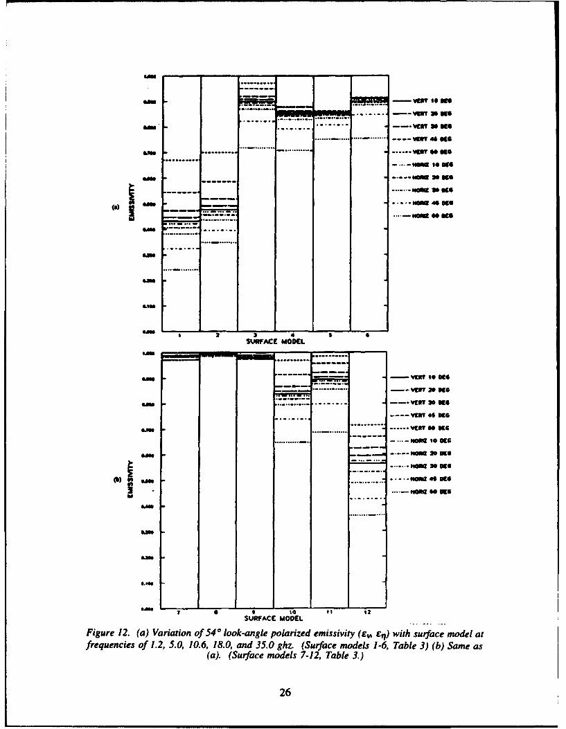
Figure 12 illustrates surface emissivities calculated for the models in Table 3 at
frequencies of 1.2, 5.0, 10.6, 18.0, and 35 ghz for a look angle of 54 degrees.
8. ISOTOPIC RATIOS
The H1TRAN database accounts for isotopic abundance by including the fractional
abundance in the line strengths. The isotopic abundances are specified on a file associatedwith the HITRAN database. With the inclusion of isotopic partition function data with theHTRAN database, the advanced spectral model has been modified to correctly describe the
strength variation with temperature for the relevant isotopic species. An individual isotopicspecies of interest is essentially treated as a separate molecule. For some atmosphericapplications, e.g. altitude dependent photodissociation of isotopic species, it would bedesirable to provide an option for treating variation of isotopic ratios in the radiativecalculation. This capability is only partially implemented in the model in the sense that amechanism is not currently available to input mixing ratio profiles for individual isotopic
species of interest. This option could be readily implemented once an approach is
established to provide the necessary but potentially extensive input data.
A copy of the Total Internal Partition Sums program (TIPS) was received from R.
Gamache, Gamache et al., 1990. A modified version of this partition function program
was incorporated into subroutine MOLEC. The capability to utilize the results from TIPS
and correctly treat the molecular isotopes was incorporated into LNFL, HIRAC1,
LNCOR I and LINF4. On comparing the results of the new model with those from the
previous version, significant divergence was encountered at temperatures greater than
400 K. After some study and discussions with R. Gamache it was established that for
some molecules an insufficient number of states were utilized in computing the partition
sums for the higher temperatures. In the current implementation of the partition function
25
... o...o....
SAN - - - - t -"
- -lugaal lem
--- Wal 2S sue�. -............. ---- 0
SA -..... ..... -.. Vff30K
.......~ ~ ........ .. .. .. --- IIv 46
... ......... ..
-NOWee. 20 age
-------lm ..... No .3. Ke
•~~ .....il blo 46 Us.+-+
•~~~4 we i. *
.............
.............
2 3 4 S 4SURFACE MODEL
--- --- -- V -0 - -
Gift ..i.i... VER G.OiiiKi.... ......... -. .I
earo - "-.... .... WSS 20) (S............ 11M.. 10 Ka
S20 we6i ... ... -...... ."Ora3 aso
(b) We.. . ..... S 4 6
e .. I....o
6 9 toI 11 ItSURFACE MODEL
Figure 12. (a) Variation of 54° look-angle polarized emissivity (ev eq) with surface model atfrequencies of 1.2, 5.0, 10.6, 18.0, and 35.0 ghz. (Surface models 1-6, Table 3) (b) Same as
(a). (Surface models 7-12, Table 3.)
26

calculation, the partition function for temperatures above 400 K is obtained by applying a
classical isotopic independent temperature dependence to the value of the partition function
at 400 K. This approach retains isotopic dependence for temperatures above 400 K.
9. INSTRUMENT FUNCTION ENHANCEMENTS
FASCODE includes the capability to convolve a monochromatic spectrum with an
instrument response function (also known as a scanning function) in order to model ameasured spectrum. This convolution can be performed either as a convolution in thespectral domain, as is currently done in FASCODE, or in the Fourier domain, usingFourier transforms. We have enhanced the instrument function capabilities of FASCODE
both by improving the existing scanning functions and by adding the capability to performthe convolution in the Fourier domain. In addition, we have improved the efficiency of theinterpolation routines.
9.1 Scanning Functions in the Spectral Domain
As a result of interactions with the U. of Wisconsin group, new scanning functions
for sinc and sinc**2 have been developed and implemented in FASCOD3. The bound forthese scanning functions has been extended to the proper value and the SHRINK function
has been correctly applied so that the scanned spectra is consistent with the result that
would be obtained if the calculation were performed in the fourier domain. The sampling
interval used for the shrink algorithm is one-eighth the halfwidth of the scanning function
for all functions. The effective bound for the sinc function is 119 halfwidths and for the
sinc**2 function is 54 halfwidths. The area under the respective functions is effectively
unity. A negative aspect of using the sinc function is the large bound associated with the
function. For the HIS spectra with an unapodized halfwidth of 0.25 cm-1 , the bound is
30 cm-1 which requires that the calculated spectrum must extend 30 cm-1 beyond the
spectral region of interest at each end of the spectrum. Nevertheless the higher resolution
associated with the sinc function is a much more critical test of the spectroscopic results
than can be obtained with other functions. The algorithm as it is coded performs the
calculation with remarkably good efficiency.
27
9.2 Scanning Functions in the Fourier Domain
Nowadays, most measurements of infrared spectra both in the lab and in the
atmosphere are made with Fourier Transform Spectrometers (FTS). Examples of
atmospheric measurements with an FTS are the Stratospheric Cryogenic Infrared Balloon
Experiment (SCRIBE) (Murcray et al., 1981), and High Resolution Interferometric
Sounder (HIS) instruments (Smith et al., 1979). These instruments are characterized by
high spectral resolution (up to 0.06 cm- 1) and large signal-to-noise. The AFGL line-by-
line model is an ideal tool to provide simulations of spectral radiance at these spectral
resolutions to aid in the identification of lines, perform retrieval studies, and to investigate
phenomena such as line mixing (Hoke et al., 1988).
The spectral response function or "scanning function" of an FTS is nominally a sinc
function, but can be modified by "apodizing" the interferogram: the scanning function is
the Fourier Transform of the apodization function. The effect of apodization is to reduce
the side lobes of the scanning ".,nLdon at the expense of broadening the central peak.
When comparing calculated spectra with spectra measured with an FTS, it is important to
accurately model the effects of the scanning function, including the side lobes.
Previously, FASCODE has performed the spectral smoothing as a convolution in
the spectral domain. The accuracy of this approach depends upon the spectral extent (i.e.
number of side lobes) over which the scanning function is defined. However, for a
convolution, the computational time increases with the spectral extent, and for accurate
calculations, can become large. We have developed a technique to perform spectral
smoothing in the Fourier domain. This technique directly mimics the operation of an FTS:
the calculated spectrum is transformed into an "interferogram", "apodized", and then
transformed back to the smoothed spectrum. With this method, all the side lobes of the
scanning function are preserved.
This technique has been implemented in a set of routines called FFTSCAN. The
user is given the choice of a number of commonly used FTS scanning functions, and may
specify the resolution either in terms of the width of the scanning function or in terms of the
maximum optical path difference of an equivalent interferometer. As an option, the input
spectrum may be prescanned with a narrow rectangular scanning function, leading to large
savings in computational time and storage at negligible cost in accuracy. The routines may
28

be run as a stand alone program or added to FASCODE as an option. This work is
reported on more fully in a separate report (Gallery and Clough, 1992).
9.2.1 Theory
In Fourier Transform Spectroscopy, the spectrum S is obtained from the
interferogram I from:
S(u) = F ( A(x) I(x)) (1)
where F indicates the Fourier Transform, A(x) is the apodization function, u is thewavenumber and x is the optical path difference. By analogy, FFTSCAN calculates the
smoothed spectrum S' from a monochromatic spectrum S as:
S'(u) = F ( F (R). F (S)) (2)
where R(v) is the scanning function. Here, F (S) is equivalent to the interferogram and
F (R) performs the role of the apodization function A. A fundamental theorem of Fourier
Transforms states that:
F ( F (R). F (S)) = R * S (3)
showing that Equation 2 is the same as a convolution in the frequency domain (* indicates
convolution).
The program offers a choice of five scanning functions commonly used with an
FTS. These scanning functions, along with their associated apodization functions, are
shown in Figure 13. For compatibility with previous versions of FASCODE, therectangle, triangle, and gaussian scanning functions are also offered. The user may specifythe width of the scanning function either as the half width at half maximum (HWHM) or as
the maximum optical path difference of an equivalent interferometer.
The user is given the option of pre-scanning the input spectrum with a rectangular
scanning function which is narrow compared with the selected scanning function(boxcaring). The pre-scanned spectrum is then resampled onto a coarser grid resulting in a
large reduction in the number of points. Subsequent processing is then performed on thereduced spectrum. This procedure can result in large (orders of magnitude) savings incomputational time and storage. The distortion of the resulting spectrum is small and can
be partially corrected by "deconvolving" the reduced spectrum.
29

Scanning Function1.0
Sinc0.8 . Sinc
--- Beer0.6 -........... Hamming
Hanning~0.4- i
E 0.2
0.0
-0.2
-0.4 . .
0 1 2 3 4 5Wavenumber (cm*)
Apodization Function1.0 ..
0.8
0.6-
E- 0.4D "'\. -..
0.2 .
0.0
0.0 0.5 1.0 1.5Displacement (cm)
Figure 13. The Five FTS Scanning Functions and Their Associated Apodization FunctionsAvailable in FFTSCAN. The maximum displacement of 1.374 cm corresponds to the HIS
instrument.
30
A FASCODE calculation can contain millions of points, more than can be storedand transformed in memory. A disk-based FFT routine was obtained from Mark Esplin ofStewart Radiance Lab, Bedford, MA, which can transform an array of arbitrary size.Using this routine, the FITSCAN can smooth a FASCODE spectrum of any size. Thecomputational time for the disk-based FFT is no more than three times that of an in-memory FFT of the same size. The program decides which routine to use - disk-based or
in-memory-based upon the size of the spectrum and available memory.
9.2.2 Examples
Figure 14 shows an example of a FASCODE spectrum smoothed usingFFTSCAN. The calculated spectrum models the upward radiance at 72 krn for the USStandard Atmosphere. The monochromatic calculation extended from 600 to 800 cm-1
with a d• of 0.000953. In Figure 14a, the monochromatic FASCODE spectrum was
smoothed with a sinc scanning function of HWHM = 0.21926 cm-1, corresponding to theHIS resolution. Figure 14b shows the error in the scanned spectrum from using boxcaringwith deconvolution. In this case, boxcaring results in a 38 fold reduction in the number of
points in the spectrum. The maximum error of about lxlO-8 is about 0.5 percent of thetypical spectral excursion of 2x 10⁻⁶ or about 0.2 percent of the maximum spectral value of
8x10⁻⁸. For reference, Figure 14c shows the error using the standard FASCOD3convolution with a bound of 119 halfwidths. The reference spectrum for calculating theerrors in Figures 14b and 14c is the FFrSCAN calculation without boxcaring, interpolated
to the proper grid.
Table 4 compares the computational time and maximum error for the calculations
shown in Figure 14. The calculations were performed on an Sun SPARC station 2 and the
scanning functions were applied from 625 cm-I to 775 cm-1. The results for scanning
with the sinc2 and the triangular scanning functions are also shown. Note that the
boxcaring errors for the other functions are four times less than that for the sinc function.
These results show that for the sinc function, FFTSCAN with boxcaring provides a
three-fold increase in speed and a better than two-fold increase in accuracy over the
conventional FASCODE scanning routines. For the sinc2 and the triangle, the execution
time for the two programs is about equal, but FFTSCAN is again twice as accurate. The
reference spectrum for calculating the errors is again the FFTSCAN calculation without
boxcaring, interpolated to the proper grid.
31

Spectrum Smoothed with FFTSCAN
8.10-5 .
6- 4.10"6
i-.2.1046
a. sinc
650 660 670 680 690 700
Error in FF MSCAN Due to Boxcatng4.108
I 2,10.8
0
-4.10"8 b.
"4"10"8 _.___--I
650 660 670 680 690 700
Difference Between FFTSCAN and FASCODE6,10-8 - -. . . . . . . . . . . . . . .-- -- -------...
2-10-4
-2-10 4
I;
-4-10-8 C
-4&10-8 c
650 660 670 680 690 700Wavenunmer (cm")
Figure 14. (a) FASCODE Calculated Spectrum Smoothed by FFTSCAN Plus The Error In theSmoothed Spectrum from using: (b) FFTSCAN With Boxcaring, and (c) the FASCODE3
Scanning Function. The scanning function is a sinc with a HWHH of 0.21962 cm"1,corresponding to the HIS instrument in the unapodized mode.
32

Table 4. Comparison of Computational Time and Accuracy, FFTSCAN versusFASCODE, for the Sinc, Sinc2, and Triangle Scan,-:.ig Functions.
Computational Time Maximum Error
(sec) (Percent Radiance)
Scanning Option Sinc Sinc 2 Triangle Sinc Sinc 2 Triangle
FFTSCAN, No Boxcar 117 117 117 (NA) (NA) (NA)
FFTSCAN, With Boxcar 5.8 3.7 3.3 0.2 0.05 0.05
FASCODE3 Convolution 17.9 3.9 3.0 0.5 0.1 0.1
Notes:
a. The computational times refer to a Sun SPARC station 2. Times are approximate
and both the absolute and the relative times will vary depending on the case.
b. The spectral extent of the smoothed spectrum was from 650 to 775 cm-1 .
c. The monochromatic di) was 0.000953 cm"1.
d. The number of points in the scanned function was 167,958 (no boxcaring) and
4419 (with boxcaring), a reduction of a factor of 38.
9.2.3 Implementation
FFTSCAN is written in ANSI Standard Fortran 77 and is designed to be highly
portable. It currently runs on a Sun SPARC station 2 but has been ported to a DEC VAX,
an CDC Cyber, and an IBM PC. The few hardware dependent parameters, related to the
disk-based FFT routines, are declared as parameters and collected in include files for easy
modification. FFTSCAN can either be run as an independent program or be included as a
module of FASCODE (called by setting ISCAN = 3). However, it has not yet actually
been incorporated into FASCODE. A detailed set of user instructions is included in the
report.
9.3 Interpolation
A new interpolation algorithm has been developed which is considerably more
efficient than the previous algorithm and provides the option of performing linear or four
point interpolation. The latter option uses continuous first derivatives, consistent with the
four point interpolation in the other FASCODE modules.
33

10. LINE SHAPE
The current limitations on the accuracy of many radiative transfer calculations is thelimitation of our knowledge of the shape of the spectral line wings. The far wing lineshape for water vapor is treated by including the line wing effects in the continuum. Forcarbon dioxide, the collisionally-broadened line wings are dependent on quadrupole-quadrupole interactions giving rise to line wing effects closer to line center. This precludes
incorporation of wing effects in the continuum as the continuum is defined in the advanced
spectral model. There are two important aspects of the line broadening problem that need
to be considered for a proper treatment of atmospheric absorption by carbon dioxide:
duration of collision effects and line coupling effects. In principal these effects should be
treated together. In reality the problem is sufficiently complex that treating them
independently is difficult enough and for most purposes reasonable results can be obtained
in the context of the known physical constraints.
10.1 Line Shape for Carbon Dioxide
The carbon dioxide line shape that has been used in the spectral model was deduced
from measurements by Burch in the 2400 cm- 1 band head. Recent comparisons with other
models and with the data discussed in Section 13.1 suggest that the sub-lorentzian character
of the carbon dioxide line shape currently being used is too strong. The line shape is given
by the expression
f(v) = L(v - v,,) X(I v- V0 )with
L(v - v)-•)aYr(v - v,,)' +ac'
where L(v - V") is the impact line shape with ac the collisional halfwidth, vo the
transition wavenumber value, and z(Ov - v.1) is a function generally referred to as the chi
factor, which provides the necessary correction to the impact line shape to obtain agreement
with observed line wing effects.
For the advanced spectral model, the implementation of the strong sub-lorentzian
behavior appropriate to carbon dioxide requires the application of a chi factor x° (0 - V,to the fourth function (Clough et al., 1981), where X' is defined through the relation
34

1+C2 (V- V0 )2 +C, (v- vo)+C 6 (v- v) 6' IV- vQI
(I - vol) = Dex(alV - Vtb) IV-IV2
where we have utilized values for the constants obtained from the work of Burch and
collaborators,
a = 0.623
and
b = 0.410.
The coefficients C2, C4, C6 and D are chosen to provide continuity of the chi
function for the value and the first two derivatives of the function at wavenumber value Vo.
The total chi factor for the line Z (Iv - V.1), in the context of the present model, is
given by the expression
x(IV- V.) =
where Q.(Iv - vQl) is a polynomial used in the line shape decomposition. In Figure 15 we
indicate the chi function for carbon dioxide previously implemented in the spectral model
for which Vo = 2 cm-1. One of the significant drawbacks to the present formulation is that
the chi function is pressure dependent and in Figure 16 two chi functions are provided, one
with ac = 0.08 cm-1 which corresponds to atmospheric pressure and one with oa = 0.008
cm-1 corresponding to one-tenth atmospheric pressure. The carbon dioxide line shape is
readily modified in the spectral model through the choice of V0 . In Figure 16 we provide a
new recommended chi function obtained with Vo = 8 cm-l. This provides a result that is
less pressure dependent, has an integrated value for the line shape closer to unity, and is
consistent with the data against which we have made comparisons.
The bandhead of carbon dioxide at 2385 cm-1 is an interesting spectral region
particularly from the point-of-view of its importance for remote sensing of temperature. It
has been proposed that line coupling plays an important role in the valleys between spectral
35

.0.6
z
€.)z
~0.4-
0.2
0.0 -0'°. - . " 16.- 21 •."- 2.SWAVENUMBER DIF
Figure 15. The chi function for carbon dioxide with Vo = 2 cm-. The solid line is forhalfwidth of 0.08 cm-n (I atm) and the dashed line is for a halfwidth of 0.008 cm- (0.1 atm).
1.0-
0.6"
z0
o.&z
S0.4--
0.2-
d. o s'. It ... ,is . 2t. 2ý.WAVENUMBER DIF
Figure 16. The chi function for carbon dioxide with Vo = 8 cm-. The solid line is forhalfwidth of 0.08 cm"! (1 atm) and the dashed line is for a halfwidth of 0.008 cm"! (0.1 atm).
36

lines in this band and particularly at the bandhead. However, performing accelerated line-
by-line computations including line coupling effects with spectral lines spanning a broad
range is problematical. Consequently it is presumed that a judicious choice of chi function
will satisfactorily describe the absorption in this region. In Figure 17 we show the
calculated transmittance for a limb calculation for two values of Vo: Vo = 2 cm-1 and Vo =
8 cm-1. The tangent height for this case is 20.5 km. The results are substantially the same.
In Figure 18 we provide an ATMOS limb occultation spectrum (R. Zander, private
communication, 1988) with a 17.7 km tangent height. The absolute values for the
transmittance are in some doubt in this spectrum so it is not feasible to perform a detailed
analysis with this particular data set. A calculation with Vo = 2 cm-1 , shown in Figure 19,
provides a result which while in marginal agreement with the observation cannot really be
considered satisfactory. It should be noted that an instrument function consistent with the
ATMOS data was not available so that the lines appear with greater amplitude in the
calculation. Based on the previous considerations, a calculation with Vo = 8 cm-1 would
provide substantially the same result. There are three effects contributing to the absorption
in the spectral region of disagreement: carbon dioxide line shape including line coupling,
the collision induced band of nitrogen, and the water vapor continuum. Improved data is
really necessary to facilitate the analysis of these effects.
A final comparison was performed between calculations with the different chi
factors for a case in the 690 cm-1 region from the ITRA exercise. In Figure 20 is shown
the transmittance spectrum for a 30 km tangent height with Vo = 2 cm-1 and in Figure 21
the result with Vo = 8 cm-1 . Here a difference is discernible in the spectral valleys between
the lines.
10.2 Line Coupling for Carbon Dioxide
Because of the importance for remote sensing of the carbon dioxide Q-branches in
the spectral region from 600 cm-I - 800 cm-1 , a concerted effort has been devoted to the
refinement and validation of the model in this spectral region particularly with respect to the
Q-branches. Our efforts have proceeded directly along the lines described by Hoke et al.
(1988) and the reader is referred to that paper for details of the approach. In the present
report we describe the validation of the coupling coefficients and the rationale for a
proposed refinement. The Q-branches of principal interest occur at 618, 720, 740 and794 cm-1.
37

WIAVELEGTH (ICOIETER I.04.64.16 4.14 4.12 4.10,.no ,.ADL . .=,z
1.0. 1.0
0..6
SO.s' 0.6
0.4, 0.4
a. 0.2 0O.z
0.0- 0.02MG 2iN 2;00 2410 2;20 2420 240 2420
WAVENWUBER (CM-1)
WVIE.EN0TH (MICRPE•TERI4.=0 4.18 4.16 4.14 4. IZ 4.10
1.0 1.0
0.93 0.6
0.6 0.6
0.4 .0.4
b. 0.2 0.2
0.0 0.0z280 n2D 2400 2430 2420 24-0 2440 241D
WAVENWUER (CM-- II
Figure 17. (a) Calculated limb transmittance spectrum with Vo = 2 cm-'; (b) Calculated limbtransmittance spectrum with Vo = 8 cm-'.
38
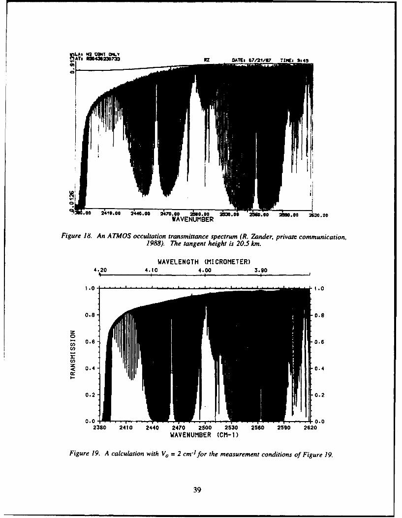
LAt N42 COWT 0IYATs 150438230733 RZ DATE# 07/21/87 TZNEs Sa49
C!
.00 2410.00 2440.00 2470.00 2500.00 20.00 2560.00 260.90 260. 00WAVENUMBER
Figure 18. An ATMOS occultation transmittance spectrum (R. Zander, private communication,1988). The tangent height is 20.5 kIn.
WAVELENGTH (MICROMETER)4.20 4.10 4.00 3.90
! .0 1.0
0.8 0.8
zu• 0.6 0.6
< 0.4 0.4I--
0.2 0.2
0.0 0.02380 2410 2440 2470 2500 2530 2560 2590 2620
WAVENUMBER (CM-1)
Figure 19. A calculation with Vo = 2 cm-1 for the measurement conditions of Figure 19.
39

iEd VTH (hICFT!R 314.W14 Am 34.4 4.4& 14.40
1. •, 1.0
aA- -0.6
0.6. 0.6
0.4. 0.4
0.2• -0.2
0.0 0.0m8 B mi ma mB mB
AVENUMBEER (01-13
Figure 20. Limb transmittance spectrum for the conditions of the ITRA intercomparison witha 30km tangent height for Vo = 2 cm-.
TAV'LDOH (mICROPETER i14. 14,M 34"S 14.44 14.40
1.0 " , .0
0.8 -0.1
0.6 0.6
i 0.4, 0.4
0.2 0.2
AYVENUtDER (C0-13
Figure 21. Limb transmittance spectrum for the conditions of the ITRA intercomparison witha 30km tangent height for Vo = 8 cm-.
40
The initial data that were used for the validation were from a nadir viewing spectral
radiance measurement made with the HIS instrument, Smith et al. (1983), from the ER2
aircraft flying at 19.6 km over ocean on April 14, 1986. A summary of the experiment and
an initial analysis of the data was given by Clough et al. (1988). In Figure 22 we indicate
the spectral residuals from 600 - 800 cm-I in terms of equivalent brightness temperature for
a validation with 1992 HITRAN parameters and no line coupling. The residual at 667 cm-I
is due to warmer gas in the vicinity of the instrument and not to line coupling. With respect
to the line coupling, Figure 22a provides a result similar to that given in Figure 26 but for
the smaller spectral range. In Figure 22b we indicate the residuals obtained with the line
coupling coefficients provided by Hoke et al. (1988 and private communication). Although
a substantial improvement has been obtained, the residuals associated with the Q-branches
are apparent and unacceptably large for remote sensing problems. In the course of study-
ing this problem it became apparent that if the coupling coefficients, both the y's and the
g's, were scaled by a multiplicative factor of 1.3, a much improved result was obtained.
This result is provided in Figure 22c. In the calculation of the coupling coefficients, a
combination of the energy power gap and exponential gap have been used to obtain the
elements of the rate matrix. The coefficients of the energy gap expressions have been
obtained by performing a least squares fit to the carbon dioxide halfwidths. This is far
from a rigorous procedure for obtaining the rate matrix elements so that from our perspec-
tive the need to scale the coupling coefficients is not inconsistent with the physics. It
should be noted that a single scale factor provides an improved result for the three Q-branch
regions at 618, 720, and 740 cm-1. This provides support for the proposition that the ef-
fect is due to the line coupling parameters and not to an artifact of the measurement or to the
errors in the description of the atmospheric temperature field. The Q-branch at 740 cm- I is
associated with a much warmer temperature than the 618 or 720 crrr 1 Q-branches. The
residuals for the 794 cm-1 Q-branch are only marginally effected by inclusion of line
coupling effects, primarily because of residuals associated with other species.
After discussion with scientists at the Phillips Laboratory, the value of performing a
similar validation using a zenith ground based observation became apparent. Data from
1 November 1988 taken as part of the GAPEX experiment by the U. of Wisconsin
researchers (Knuteson et al., private communication) have been utilized. This validation
provides a second observation with a significantly different temperature field with respect
to the optical path. The results are provided in Figure 23. The results for the 618, 720,
and 740 cm-1 Q-branches fully support the scaling factor of 1.3. In the course of this
41

-2.0 zo
4*.. 1 W0.
3.0
&a 0.0
10.0 Mo 0. .
't0 it. le
S.6.0
3-1.
b. ,
-1.4. -.
000 02 o 640 60 41o 1 2 1"1 7f me0 f0
VAVINGIFM (ffCROOdMC5)
10.0 5.0560 9
Se.0 S....( 0..
-. o .4.
4.0 .O
0 h4
6..4
oo 420 .0o W1 M Too1 ?" noe 909
WAVWPMU0 (CM-i)
Figure 22. Effect of line coupling on the spectral residuals for the nadir HIS observation of14 April 1986: a) no line coupling, b) line coupling with the basis coupling coefficients, and
c) basis coupling coefficients multiplied by a factor of 1. 3.
42

WAV*•L•NGTH 4.KSWOATEaR)
N.Ss0.0 .
-A, Ia.
--.*
irAVENIMSCR (¢v- 1)
WAVELEN4GTH' (WCMOKilTg.)-2.5 3.0
1.. 5 l .0- , S
,AVIeCGTO e f SCT .
A.5 2.5
Pr2w- 0 .V45
b. *
-2.0
-2.5 -S.5
WAY RUMOC (C0-1)
WAVELENGTH OHMEtuTER)
2.3
2.0 6
0.00
, U,,, , r. 05
C. .5.o. -e55
-2.0 5.
-A E..S 0 g, ( C .-
Figure 23. Effect of line coupling on the spectral residuals for the zenith observation of INovember 1988 with the HIS instrument: a) no line coupling, b) line coupling with the basis
coupling coefficients, and c) basis coupling coefficients multiplied by a factor of 1.3.
43

study, an adjustment of the temperature dependence of the coupling coefficients was
explored to ascertain whether equivalent results could be obtained. Consistent with the fact
that the different Q-branches are influenced by different temperature regimes in the atmo-
sphere, no simple adjustment of the temperature dependence could provide an equivalent
result. The spectral residuals associated with the P and R branches of the 618 and
720 cm-1 carbon dioxide bands as seen in Figures 22 and 23 are of particular note. These
residuals, up to ±2K in brightness temperature for the nadir, are the largest residuals in this
measurement band. It has not been possible to obtain an improved result with a retrieved
atmospheric temperature profile, suggesting that the errors are spectroscopic in nature.This conclusion is supported by a plot of the residuals from 680 -780 cm-I of Figure 22
against equivalent brightness temperature as provided in Figure 24. The lack of correlationimplies that there is no adjustment of the atmospheric temperature field that can provide an
improved result.
5 ," , . . I i | I * I I
2 4- 4-2 + +
+ + 4-
+ 4. + + +
4 W 4. + +
+ ++ ++ +*+4 ++ + + ++
++ + + *4. 4- + + 4-
+ ++ + ++ + ++.• 4. ÷ 4.4. +4. .
,a. 4+ " +" + 4. + + •+ +
+ +++.
0 "IIT4. + + • +÷ .. +. /++ 4 ",.
+"� +++ + ++ + ++++ + ++ + + +-, + + +-•
+ " + .
-24.3.
MO 220 20 260 280 300Rd (K)
Figure 24. Brightness temperature residuals associated with Figure 22c as a function ofbrightness temperature.
44
11. COLLISION INDUCED BANDS
As a result of recent theoretical and experimental considerations, it is possible to
attain some improvement in the treatment of a number of collision induced bands important
to atmospheric radiative transfer modeling. The collision induced bands of particular
interest include the nitrogen band in the pure rotation region, the oxygen band at 1600 cm-t
and the nitrogen band at 2350 cm-I with important contributions at 2400 cm-1.
With respect to the collision induced nitrogen band at 2350 cm-1, the best current
validations appear to be associated with the ATMOS experiment in which it is possible to
study the absorption in the spectral region from 2400 - 2600 cm-1 as a function of tangent
height (e.g. Figure 18). As a result of studying ATMOS spectra for 20.5 and 17.6 km
tangent heights and given the uncertainty in the far wing line shape of carbon dioxide which
impacts the absorption beyond the bandhead at 2385 cm- 1, a modification of the nitrogen
continuum currently in the model does not seem warranted at the present time. It should be
pointed out that the ATMOS spectra test both the pressure and temperature dependence of
the model, although not independently.
With respect to the collision induced oxygen band at 1600 cm-1, we have imple-
mented the modification proposed by Rinsland et al., 1989. This modification involved the
application of a multipicative scale factor of 0.78 to all values of the oxygen continuum.
The analysis of Rinsland et al. (1989) was also based on results from the ATMOS
occultation experiment (R. Zander, private communication, 1988).
12. SPECTRAL MODEL ENHANCEMENTS
A review of the advanced spectral modeling developments implemented for FASCODE
under this effort are summarized below. A number of these topics are covered in greater detail
in other sections of this report, but are included here for completeness.
CURRENTLY IMPLEMENTED INTO FASCODE
LINE-BY-LINE CALCULATION
Interpolation error corrected (affected interpolation of aerosols, thecontinuum, and the fourth function, at the ends of the panel)Implementation of the impr-ved radiance algorithm (uses leveltemperatures)
45

SCAN/INTERPOLATION UPDATES- Error in SHRINK fixed (related to wavenumber shifts)- RECTANGLE function updated- SINC function updated with new bound- SINC**2 function updated with new bound- Input option for first zero crossing of periodic functions- Input option to specify the output spectral spacing- Input file is first interpolated before being scanned when input DV is too
coarse- INTRPL rewritten (four-point interpolation scheme added)
CROSS-SECTIONS FOR HEAVY MOLECULES- Extinction effects of heavy molecules (HITRAN '86)- Lorentzian convolution over the cross-sections to account for pressure-
dependence effects- Temperature-dependent cross-section data from HITRAN '91 can also be
used- Atmospheric trace profiles from 'AER/NASA community model'
PARTITION SUMS- Program TIPS from Gamache and Rothman incorporated- Isotopic species now treated correctly within FASCODE- Problem with partition sums at high temperatures addressed (Gamache and
Rothman currently investigating)- TESTMM was also modified to set the isotope for all lines contained in the
block data set to 'T'.
LINE COUPLING- Line coupling coefficients on TAPE3 at four temperatures are required
(200 K, 250 K 296 K and 340 K)- Files: CPLDT & CPLDTl3/UN=ISAACS (9 Nov 1990)- Current implementation is compatible with HITRAN '91- The line-coupling coefficients for 02 were updated and integrated back into
LNFL and BTEST
FLUX CALCULATIONS
- Heating rate routines provided in FLUXF/UN=ISAACS (9 Nov 1990)
FSCATM- Level temperatures and pressures provided on TAPE7 output- Cross-section profile capability added
LOWTRAN7/AEROSOLS
Fix to V l, V2 (AV l, AV2 in LOWTRN) on FILHDROption added to allow input of precalculated aerosols
46

SEQUENTIAL TRANSMIT'ANCE/RADIANCE
Total transmittances/radiances from observer to successive layersExtensive improvements have been made in the sequential calculationoption, formerly called the weighting function option. Sequential radiancesmay now be obtained, an option that is necessary for the calculation offluxes and heating rates. The improved interpolation algorithm has beenadapted to perform more efficient interpolations in the course of the mergingcomputations for transmittance and radiance.
REFLECTED ATMOSPHERE
- Option to include the effects of atmospheric radiation reflected by the earth'ssurface
- Spectral variation of reflectivity and emissivity (quadratic in wavenumber)
PLOT PACKAGE ENHANCEMENTS - ACCESS TO FORMATITED RESULTS- The output of the plot header is now an option- Optional formatted output file- FASCODE formatted output plot file- File difference/ratio option- Plot overlays with offsets- Interface to NCAR routines
ENHANCED PORTABILITY
- Hollerith data statements have been replaced with character strings- UNIX date and time calls provided
NEW DEFAULTS
The default for the average air broadened halfwidth (ALFALO) has beenchanged to 0.08 cm-1 for the case of no line coupling. Suggested value forALFALO is 0.04 cm-I for the case with line coupling.Default values for line rejection may be invoked using negative values iorDITMIN and/or DPTFAC. The default values are
0.0002 for DPTMIN0.001 for DPTFAC
The default values for the boundary temperature differential for FSCATMhave been changed to
8 K at altl12 K at alt2
LNFL - LINE FILE CREATION PROGRAM
- Molecules expanded to 35 (from 28)- Isotope information now included in molecule variable- Fully compatible with HITRAN 91- Flag on header indicates presence of isotopic information
47

USER DOCUMENTATION
User Instructions for FASCODE and LNFLDescription of routines and input parametersBlock Diagrams of FASCODE and LNFL
Additional Issues related to FASCOD3 -
J.C. Chetwynd (PUGP) and R.D. Worsham (AER) met in late June andconfirmed that the changes which had been made in the AER code, werealso in the PL/GP version of the code.
13. ADVANCED SPECTRAL MODEL VALIDATION
13.1 Validation with Data from the High-resolution Interferometer Sounder (HIS)
A detailed comparison between measured and calculated upwelling radiances has
been undertaken to validate both the results from the High-resolution Interferometer
Sounder, HIS, (Smith et al., 1983) and to validate the performance of the advanced
atmospheric radiance model. This constitutes an important step in establishing the extent of
the retrieval improvement attainable with the HIS instrument operating in space. Special
emphasis has been placed on atmospheric spectroscopic issues associated with line
coupling; the line shape for carbon dioxide; and atmospheric window absorption including
effects due to water vapor and chlorofluorocarbons in the 800 to 1200 cm-I region.
The HIS is an accurately calibrated Fourier Transform spectrometer developed to
measure infrared radiances. The important characteristics of the instrument are summarized
in Table 5 and described in detail by Revercomb (1987). Accurate radiometric calibration
has been a central focus of the HIS program and is achieved by using two blackbody
calibration sources, one at 300 K and the other at 245 K. In the validations described here,
a correction has been applied to the measured the interferogram to account for a small finite
field-of-view effect. This correction has been applied by the U. of Wisconsin workers and
has facilitated the validation with the spectral model. Finally, a Fourier transform is
performed to obtain the spectrum. No additional apodizing function has been applied to the
data described here so that the effective apodizing function is a rectangle in the
interferogram domain providing a sinc scanning function in the spectral domain. The
calculated spectral radiances are obtained using the sinc scanning function at the identical
spectral values as the calibrated experimental spectra.
48

Table 5. Characteristics of the HIS Instrument for Flight of 14 April 1986
Spectral RangeBand 1 590 - 1070 cm-Band II 1040 - 1930 cm-1
Band III 2070 - 2750 cm-Platform ER2Altitude 19.6 kinView nadirSurface oceanInstrument temperature ambientResolution (hwhm) 0.365 cm-1
absolute - 1 Krelative 0.5 K
The particular data set we have utilized in this validation is from an ER2 flight over
the ocean off the California coast on April 14, 1986. This data set has been chosen
primarily because of the greater confidence in the characterization of the ocean surface
properties relative to those for land surface. The calibrated spectral radiance in units of
equivalent brightness temperature for the measurement set to be studied is shown in
Figure 25. An input atmosphere for FASCODE developed by R. Knuteson at the
University of Wisconsin is provided in Table 6. The temperature and water vapor profiles
were obtained from routine local radiosonde measurements while profiles for the other
molecular species were obtained from the U.S. Standard atmosphere. The mixing ratio for
carbon dioxide has been taken as 345 ppmv. The surface emissivity has been taken as 1.0
and the surface temperature has been obtained from the equivalent brightness temperature in
the spectral window since an independent measurement of the surface temperature was not
available.
In Figure 26 we show the difference between the HIS measurement and a
FASCODE calculation performed using this 24-layer atmosphere and the 1986 H1TRAN
database (Rothman et al., 1987). The agreement is generally satisfactory, but a number of
spectroscopic issues are clearly evident. The large positive residuals at the 618, 720,
49

Table 6. The Input Atmosphere for the Validations in FASCODE Format
$ CALCULATION OF TRANSMITTANCES FROM RADIOSONDE NO. 81 ALLHI=1 F4=1. CN=1 AE=0 EM=1 SC=1 FI=0 PL=0 TS=0 AM=0 MG=0 LA=0 145=0 5 5
590. 1110. 0. .0002 .001287. 1.24 7 1.000000 RAOB 72394 8610 H1= 19.67 H2= .00 ANG= 180.000 LEN= 0
974.98 286.07 1 .00 1000.00 286.91 .43 950.00 285.228.778E+21 3.668E+20 2.878E+16 3.404E+17 1.584E+17 1.808E+18 2.223E+23 8.323E+23
934.99 284.93 1 .70 920.000 284.643.308E+21 2.197E+20 1.779E+16 2.038E+17 9.375E+16 1.083E+18 1.331E+23 5.003E+23
884.95 283.41 1 1.36 850.000 282.164.423E+21 5.130E+20 4.354E+16 4.760E+17 2.155E+17 2.529E+18 3.109E+23 1.172E+24
814.93 280.42 1 2.06 780.000 278.642.603E+21 5,122E+20 4.638E+16 4.753E+17 2.100E+17 2.525E+18 3.104E+23 1.172E+24
739.87 276.03 1 2.94 700.000 273.363.158E+21 5.860E+20 5.499E+16 5.438E+17 2.335E+17 2.889E+18 3.551E+23 1.340E+24
684.98 272.19 1 3.29 670.000 271.001.542E+21 2.193E+20 2.099E+16 2.035E+17 8.549E+16 1.081E+18 1.329E+23 5.014E+23
644.94 268.99 1 3.90 620.000 266.952.581E+21 3.664E+20 3.519E+16 3.399E+17 1.408E+17 1.806E+18 2.220E+23 8.374E+23
595.68 265.04 1 4.53 571.470 263.102.476E+21 3.552E+20 3.521E+16 3.296E+17 1.350E+17 1.751E+18 2.153E+23 8.119E+23
535.59 259.66 1 5.55 500.000 256.112.634E+21 5.233E+20 5.564E+16 4.856E+17 1.975E+17 2.580E+18 3.172E+23 1.197E+24
487.48 254.85 1 5.93 475.000 253.597.576E+20 1.830E+20 2.099E+16 1.698E+17 6.861E+16 9.019E+17 1.109E+23 4.187E+23
452.42 251.03 1 6.67 430.000 248.421.179E+21 3.293E+20 4.110E+16 3.056E+17 1.219E+17 1.623E+18 1.996E+23 7.538E+23
414.96 246.55 1 7.19 400.000 244.663.487E+20 2.193E+20 3.07(--16 2.036E+17 7.954E+16 1,081E+18 1.329E+23 5.026E+23
374.88 241.34 1 8.13 350.000 237.922.451E+20 3.659E+20 5.902E+16 3.395E+17 1.279E+17 1.801E+18 2.217E+23 8.385E+23
324.85 233.85 1 9.19 300.000 229.669.570E+19 3.659E+20 8.125E+16 3.391E+17 1.194E+17 1.797E+18 2.217E+23 8.387E+23
274.82 224.99 1 10.39 250.000 220.162.951E+19 3.656E+20 1.291E+17 3.371E+17 1.079E+17 1.788E+18 2.216E+23 8.383E+23
224.83 215.91 1 11.80 200.000 211.461.131E+19 3.654E+20 2.425E+17 3.323E+17 9.354E+16 1.774E+18 2.215E+23 8.380E+23
175.04 212.53 1 13.59 150.000 213.719.022E+18 3.661E+20 3.753E+17 3.252E+17 7.213E+16 1.752E+18 2.218E+23 8.392E+23
142.55 213.49 1 14.24 135.108 213.253.793E+18 1.088E+20 1.467E+17 9.476E+16 1.623E+16 5.136E+17 6.595E+22 2.495E+23
125.04 212.19 1 15.25 115.000 211.075.149E+18 1.471E+20 2.117E+17 1.263E+17 1.798E+16 6.874E+17 8.920E+22 3.374E+23
107.50 211.16 1 16.11 100.000 211.263.824E+18 1.097E+20 2.116E+17 9.221E+16 1.064E+16 5.056E+17 6.648E+22 2.515E+23
92.509 211.99 1 17.12 85.0000 212.764.i,98E+18 1.097E+20 2.445E+17 8.975E+16 8.615E+15 4.978E+17 6.650E+22 2.516E+23
77.498 212.61 1 18.33 70.0000 212.456.108E+18 1.097E+20 2.765E+17 8.593E+16 6.725E+15 4.868E+17 6.650E+22 2.516E+23
65.001 212.51 1 19.29 60.0000 212.58
50

Table 6. The Input Atmosphere for the Validations in FASCODE Format
(continued)
4.917E+18 7.319E+19 2.489E+17 5.424E+16 3.481E+15 3.157E+17 4.436E+22 1.678E+2358.198 212.66 1 19.67 56.3960 212.75
2.028E+18 2.638E+19 1.471E+17 1.875E+16 1.092E+15 1.113E+17 1.599E+22 6.047E+220.21962109 600.0665 1080.009 1 4 -. 13775637 12 1 1 11 050.21962109 600.0665 1080.009 0 4 -. 13775637 12 1 1 11 05
-1.
51

W O0
UO0.O
- 240.0
200.'
W00 900 1000 1100
m•vENtIMBR (CM°-1
Figure 25. HIS equivalent brightness spectra from April 14, 1986: nadir view over oceanfrom 19.6 kmn.
16.0. 6.0
L4.0 24.0
12.0 i6.0
*i 6.0 16.0-
0.0 2 .11 2..1.
S00 7W0 go Soo 0o.
WAVENU2M•R (Cr- I I
Figure 26. The difference spectrum in equivalent brightness temperature between thespectrum of Figure 25 and a calculated spectrum using FASCODE with the 1986 HITRANline parameters. An error of ) K in the window region at 1000 cm"1 corresponds to a 1.6%
error in radiance.
52
740, and 791 Q-branches are due to line coupling. The positive residual at 667 cm-I isactually due to a short path of warmer gas in the vicinity of the instrument pod and not toline coupling in the main carbon dioxide Q-branch. The broad negative features at 795,850, and 920 cm-I are due to CC14, CFC 11, and CFC 12, respectively. Finally, thedifference between the true ozone profile and the U.S. Standard profile assumed for thiscalculation is responsible for the spectral discrepancies from 990 to 1060 cm-1 . Despite thefact that the radiosondes were not especially well located temporally or spatially withrespect to the observation, this validation based on the radiosonde data is remarkably good.
The effects of line coupling including its temperature dependence have beenaccounted for using line coupling coefficients of Hoke and Clough (1989) multiplied by afactor of 1.3 based on this and related spectra. The results are presented in Figure 27.Essential to these results are improved interim carbon dioxide line parameters provided byL.S. Rothman (1988). The improvement in the carbon dioxide line intensities arequalitatively consistent with those developed for ATMOS, Brown et al. (1987). Theresiduals for ozone have been reduced through the application of a retrieval algorithm toattain an improved ozone profile, Clough et al. (1990) and Isaacs et al. (1990). Theremaining residual associated with the main Q-branch of carbon dioxide at 667 cm-I due towarm gas near the instrument is unaffected by the inclusion of line coupling effects.
It is of interest to note in Figure 27 that the three spectral features with reducedradiance associated with CC14 at 795 cm-1, CFC 1I at 850 cm-1, and CFC 12 at 920 cm-1
are the manifestation of the greenhouse cooling effect attributable to these threeanthropogenic gases. Using the option in the advanced spectral model to treat the effects ofcross sections appropriate to the heavier molecules, we obtain the results shown inFigure 28. The option to perform a convolution to account for the difference in pressurebetween that appropriate to the atmospheric layers and the pressure at which the crosssection data are provided was not available at the time these calculations were performed.The cross sections are due to Massie et al. (1985). The profiles for the species treated,CC14, CFC1 1, and CFC 12, have been obtained from the AER 2d chemistry model, Ko etal. (1990). The broad spectral features due to the radiative effects of these molecules iswell accounted for as demonstrated in this residual spectrum.
53

t0.0 30.0
.0.0 .0
6.00 6.0
4.0 4 .0
02.0.
S 0.0 -0.0
-2.0 -2 0
-4.0 --
4.0 -6.0
-0.0 -0.0
-30.0 1 10.060O 70• 6 to00 I0O0
WAVENLJMSER (CCM-1)
Figure 27. The difference spectrum in equivalent brightness temperature between thespectrum of Figure 25 and a calculated spectrum using FASCODE with the inclusion of the
effects of line coupling and improved carbon dioxide line parameters.
040.0
6 ,0 6 I.0
6.06.
4.0 4 .0
0.0 0.0
L -. 0 -4. 0
4.0 -6.0
-10.0 ,B 1.00
60 00' SO1000 1100:
Figure 28. The difference spectrum in equivalent brightness temperature between thespectrum of Figure 25 an a calculated spectrum using FASCODE. The effect of CCI4 at 795cm"1, CFCIJ at 850 cm1j and CFCI2 at 920 cm1j have been taken into account in addition
to the effects included in Figure 27.
54
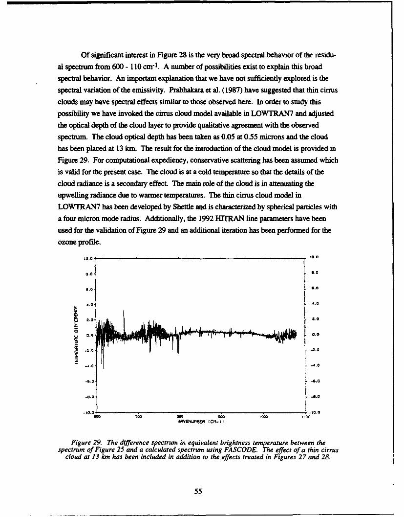
Of significant interest in Figure 28 is the very broad spectral behavior of the residu-
al spectrum from 600 - 110 cm-1 . A number of possibilities exist to explain this broad
spectral behavior. An important explanation that we have not sufficiently explored is the
spectral variation of the emissivity. Prabhakara et al. (1987) have suggested that thin cirrus
clouds may have spectral effects similar to those observed here. In order to study this
possibility we have invoked the cirrus cloud model available in LOWTRAN7 and adjusted
the optical depth of the cloud layer to provide qualitative agreement with the observed
spectrum. The cloud optical depth has been taken as 0.05 at 0.55 microns and the cloud
has been placed at 13 km. The result for the introduction of the cloud model is provided in
Figure 29. For computational expediency, conservative scattering has been assumed which
is valid for the present case. The cloud is at a cold temperature so that the details of the
cloud radiance is a secondary effect. The main role of the cloud is in attenuating theupwelling radiance due to warmer temperatures. The thin cirrus cloud model in
LOWTRAN7 has been developed by Shettle and is characterized by spherical particles with
a four micron mode radius. Additionally, the 1992 H1TRAN line parameters have been
used for the validation of Figure 29 and an additional iteration has been performed for the
ozone profile.
10.0 10.0
0.0 0.0
-6.0
U. 2,• .0
-2.
-.1.0 --. 0
.1.- -10.0
IJAVENUIMBER (CM-1)
Figure 29. The difference spectrum in equivalent brightness temperature between thespectrum of Figure 25 and a calculated spectrum using FASCODE. The effect of a thin cirrus
cloud at 13 kan has been included in addition to the effects treated in Figures 27 and 28.
55
At this stage of the validation a number of conclusions can be drawn. Perhaps the
most important concerns the high quality of the radiance spectrum, particularly when the
nature of the platform, the ER2 aircraft, is considered. The noise level in the data is of the
order of 0.1 K, the relative calibration appears to be of the order of 0.25 K and theabsolute calibration gives every indication of being better than 1 K. If Figure 29 is
compared with Figure 29, substantial improvement has been attained. The sharp,
apparently random spectral residuals throughout the spectrum are associated with watervapor. The denser more regular residuals from 600 - 780 cm-1 are associated with carbondioxide. The magnitude of the water vapor residuals is principally due to errors in the line
strengths and widths, with a contribution from the radiosonde atmospheric description.
The errors on the carbon dioxide region are apparently spectroscopic in nature and are dueto errors in the line strengths and widths. It is important to recognize that the errors being
considered here are of the order of 2% in the radiance. Also of interest is the generalimprovement in the water vapor residuals in the v2 region (above 800 cm-1) and of the
ozone residuals. These improvements in the spectral residuals are a direct consequence ofimprovements in the 1992 HITRAN line parameters.
Another important validation that has been performed is one for the same spectral
region except that the HIS spectral radiometer was on the surface at Denver Colorado
observing in the zenith mode. In Figure 30 is presented the radiance spectrum from 600 -1100 cm-1 obtained with the HIS instrument. In Figure 31 is shown a difference spectrum
in brightness temperature between the measurement and a calculation using the advanced
spectral model. For this comparison the line coupling coefficients have again been
multiplied by the factor of 1.3 consistent with the downlooking comparisons. In the
comparison of Figure 32 the cross sections for the heavy molecular species have not been
taken into account. Residuals due to CFC11 at 850 cm-1 and CFC12 at 920 cm-1 are again
apparent. In this case the effect of the absorption is to provide a positive residual, i.e. thespectral model without inclusion of cross section effects is not calculating enough radiance
in the lower layers in which the fluorocarbons are absorbing. It is of interest that for a
completely different viewing situation and a different atmosphere, many of the samespectral residual features are apparent as in the downviewing spectra: spectral residuals
associated with carbon dioxide and with water vapor.
56

WAVELENGTH (MICROMETERIS I 14 3d J 12 i1
LhJ
L .S 1.5
1.3 -1.3
U- L1 I .
S0.90. c ..wI.-
C 0.7 0.7
0.5-' O.S
m 0.3- 0.3(-
0.1 0.1
-0 ..1.1 -0.1~
S0o 700 9010 900 1000 1100WAVENUMBER (CM-i)
Figure 30. Zenith radiance spectrum observed with the U. of Wisconsin HIS instrument atDenver, CO, 1 Nov 1988, as part of the GAPEX campaign.
WAVELENGTH (M ICROMETER)16 is 14 13 12 1, 10
2.52.
S2.0 -2.04-
LiJ- 1 .5 1.6
1.0 1.0
0.5 0.S
Uj -0.0 -0.0
-0.5. -0.50:
LU -1.0 -1.0
I-1.S, -1 .S
, -2.0 -2.0
-2.5 -2.5sa0 700 Soo Soo 1000 1100
WAVENUMBER (CM-1)
Figure 31. Radiance residuals between the observed spectral radiance of Figure 30 and aFASCODE calculation with a radiosonde defined atmosphere.
57

13.2 ITRA Microwave Validation
The international campaign to study the performance of line-by-line models (ITRA:
Intercomparison of Transmittance and Radiance Algorithms) with respect to observed
atmospheric radiance data has selected a dataset from Westwater et al. (1990) for th-.
microwave region. During this reporting period, the performance of FASCODE has been
evaluated with respect to this dataset. The dataset consists of zenith radiance measurements
from the surface at three frequencies for 100 observational cases. The three frequencies are
in the atmospheric windows at 20.6, 31.65 and 90.0 ghz.
In order to perform the necessary calculations with FASCODE, modifications to the
atmospheric path computation program (FSCATM) were implemented to accommodate the
large number of levels provided with the dataset for the specification of the atmospheric
path. An abbreviated example of an input profile to the atmospheric layering program is
provided in Table 7. The associated input to the FASCODE radiative transfer calculation
obtained from utilizing the profile data from Table 7 is provided in Table 8. A study of the
sensitivity of the FASCODE calculations to the layering indicates that the layering provided
in Table 8 results in radiance calculations that are essentially invariant to finer atmospheric
layering.
Radiance results using values for the oxygen line parameters included in FASCODE
subroutine TESTMM as of I May 1991 were in poor agreement with the Westwater et al.
brightness temperatures for the specific cases examined. Using this original version of
TESTMM and a value of 2.75 K for the equivalent brightness temperature of the radiance
from space, the observed and calculated brightness temperatures for the three frequencies
were:
data of 88 10 29 1620
frequency (ghz) 20.6 31.65 90.0
observed (K) 17.66 12.32 31.23
calculated (K) 16.84 11.98 38.72
An effort was initiated to determine the cause of the rather serious disagreement at
90.0 ghz. Initial tests indicated that the sum rules on the line coupling coefficients,
including temperature dependence, were satisfied. On examining the errors associated with
58

Table 7. Abbreviated Input file for Atmospheric Layering Associatedwith ITRA Microwave Comparison
TEST CASE FOR FSCATM PROGRAM7 2 33 1 1 7 1 715.1.611 60.000 0.0001.611 2.000 2.500 3.000 3.500 4.000 4.500 5.0005.500 6.000 6.500 7.000 8.000 9.000 10 000 11.000
12.000 13.000 14.000 15.000 17.500 20.000 22.500 25.00027.500 30.000 32.500 35.000 40.000 45. 50. 55.60.
8810291620 317842.5 1.6110 7.60 -2.99 .47
842.4 1.6120 10.00 -3.31 .39
835.0 1.6850 6.90 -3.92 .46
826.3 1.7720 9.90 -4.47 .36822.4 1.8110 11.20 -4.47 .33818.3 1.8530 13.20 -3.99 .30814.3 1.8940 14.30 -3.95 .28810.4 1.9350 14.20 -4.52 .27806.1 1.9790 14.00 -4.70 .27801.8 2.0240 13.80 -4.87 .27798.2 2.0620 13.70 -4.95 .27795.0 2.0960 13.70 -4.95 .27791.6 2.1320 13.50 -5.62 .26788.0 2.1710 13.30 -5.79 .26784.5 2.2080 12.90 -5.64 .27780.6 2.2500 12.70 -5.81 .27776.6 2.2930 12.30 -6.16 .27772.6 2.3360 11.90 -6.03 .28768.6 2.3790 11.50 -5.91 .29764.6 2.4230 11.10 -6.26 .29759.9 2.4740 10.60 -6.25 .30755.3 2.5250 10.20 -6.60 .30750.7 2.5760 9.70 -6.61 .31746.1 2.6270 9.20 -6.64 .32741.5 2.6780 8.70 -6.68 .33737.2 2.7260 8.20 -7.12 .33733.0 2.7730 7.80 -7.08 .34728.9 2.8190 7.30 -7.15 .35724.8 2.8660 6.90 -7.50 .35721.0 2.9090 6.50 -7.50 .36717.2 2.9520 6.00 -7.59 .37713.7 2.9920 5.60 -7.60 .38710.3 3.0310 5.30 -7.54 .39706.7 3.0730 5.00 -7.81 39703.0 3.1160 4.60 -7.84 .40699.3 3.1590 4.20 -8.20 .40695.8 3.1990 3.90 -8.15 .41692.6 3.2370 3.60 -8.74 .40689.0 3.2790 3.30 -8.70 .41
59

Table 7. Abbreviated Input file for Atmospheric Layering Associatedwith ITRA Microwave Comparison
(continued)
685.6 3.3190 2.90 -9.06 .41682.2 3.3590 2.60 -9.02 .42678.8 3.4000 2.40 -9.51 .41675.6 3.4380 2.10 -9.78 .41672.2 3.4790 1.80 -10.06 .41668.7 3.5210 1.40 -10.11 .42
6W

Table 8. Layer Specifications Resulting from the Input File of Table 13.3
$8810291620 317 WESTWATER ET. AL. PROFILE # 1 FSCATMHI=1 F4=1 CN=1 AE=0 EM=1 SC=0 FI=0 PL=0 TS=1 AM=0 MG=0 LA=2 MS=0 XS=0 5 50.687142 0.687142 0. .0 .0
0. 1.32 7 1.000000 TWAT T. A H1= 1.61 H2= 60.00 ANG= 0.000 LEN= 0
823.34 284.25 3 1.61 842.500 280.75 2.00 804.090 287.064.453E+21 0.OOOE+00 2.600E+16 2.612E+17 1.150E+17 0.OOOE+00 1.706E+23 6.411E+23
780.84 285.64 3 2.50 757.551 283.555.063E+21 0.OOOE+00 3.234E+16 3.167E+17 1.372E+17 0.OOOE+00 2.069E+23 7.778E+23
735.31 281.17 3 3.00 713.001 278.694.646E+21 0.OOOE+00 3.131E+16 3.030E+17 1.289E+17 0.OOOE+00 1.979E+23 7.443E+23
691.73 276.70 3 3.50 670.448 274.754.170E+21 0.OOOE+00 3.009E+16 2.896E+17 1.211E+17 0.OOOE+00 1.892E+23 7.118E+23
650.10 272.42 3 4.00 629.765 270.223.539E+21 0.OOOE+00 2.899E+16 2.765E+17 1.140E+17 0.OOOE+00 1.806E+23 6.799E+23
610.36 267.93 3 4.50 590.949 266.123.133E+21 0.OOOE+00 2.861E+16 2.639E+17 1.079E+17 0.OOOE+00 1.724E+23 6.493E+23
572.50 264.55 3 5.00 554.070 263.062.043E+21 0.OOOE+00 2.869E+16 2.507E+17 1.022E+17 0.OOOE+00 1.637E+23 6.177E+23
536.52 261.07 3 5.50 518.994 258.871.562E+21 0.OOOE+00 2.853E+16 2.381E+17 9.676E+16 0.OOOE+00 1.555E+23 5.870E+23
502.35 257.12 3 6.00 485.667 255.751.456E+21 0.OOOE+00 2.830E+16 2.263E+17 9.147E+16 0.OOOE+00 1.478E+23 5.580E+23
469.95 254.45 3 6.50 454.189 252.691.244E+21 0.OOOE+00 2.880E+16 2.140E+17 8.557E+16 0.OOOE+00 1.398E+23 5.277E+23
439.28 251.25 3 7.00 424.354 249.607.317E+20 0.OOOE+00 3.013E+16 2.025E+17 7.971E+16 0.OOOE+00 1.323E+23 4.999E+23
396.86 245.83 3 8.00 369.340 242.281.034E+21 0.OOOE+00 6.287E+16 3.737E+17 1.423E+17 0.OOOE+00 2.441E+23 9.227E+23
344.72 238.91 3 9.00 320.165 235.315.368E+20 0.OOOE+00 7.735E+16 3.338E+17 1.191E+17 0.OOOE+00 2.181E+23 8.250E+23
297.58 231.54 3 10.00 275.272 228.202.316E+20 0.OOOE+00 1.012E+17 2.964E+17 9.726E+16 0.OOOE+00 1.943E+23 7.350E+23
255.82 224.09 3 11.00 236.358 219.434.738E+19 0.OOOE+00 1.404E+17 2.610E+17 7.827E+16 O.OOOE+00 1.726E+23 6.530E+23
219.02 215.26 3 12.00 201.680 212.111.127E+19 0.OOOE+00 1.925E+17 2.294E+17 6.194E+16 0.OOOE+00 1.538E+23 5.820E+23
186.62 211.10 3 13.00 171.565 210.653.277E+18 0.OOOE+00 2.205E+17 1.963E+17 4.550E+16 0.OOOE+00 1.335E+23 5.054E+23
158.82 212.35 3 14.00 146.095 213.931.210E+18 0.OOOE+00 2.373E+17 1.635E+17 3.083E+16 0.OOOE+00 1.130E+23 4.275E+23
135.24 212.56 3 15.00 124.399 210.024.044E+17 0.OOOE+00 2.626E+17 1.367E+17 2.059E+16 0.OOOE+00 9.614E+22 3.638E+23
103.60 209.46 3 17.50 82.8592 210.007.755E+16 0.OOOE+00 8.214E+17 2.516E+17 2.681E+16 0.OOOE+00 1.846E+23 6.988E+23
69.103 211.11 3 20.00 55.2944 212.397.815E+17 0.OOOE+00 1.039E+18 1.471E+17 1.077E+16 0.OOOE+00 1.222E+23 4.624E+23
46.195 213.80 3 22.50 37.1228 215.671.181E+18 0.OOOE+00 1.188E+18 8.463E+16 5.032E+15 0.OOOE+00 8.066E+22 3.053E+23
31.076 217.35 3 25.0025.0391 219.31
61

Table 8 Layer Specifications Resulting from the Input File of Table 13.3(continued)
1.813E+17 0.OOOE+00 1.127E+18 4.872E+16 3.551E+15 0.000E+00 5.339E+22 2.021E+2321.036 221.04 3 27.50 17.0328 223.430.OOOE+00 0.000E+00 9.299E+17 2.840E+16 2.642E+15 0.000E+00 3.555E+22 1.346E+23
14.353 225.74 3 30.00 11.6790 228.330.OOOE+00 0.OOOE+00 6.999E+17 1.708E+16 1.878E+15 0.OOOE+00 2.377E+22 8.994E+22
9.8708 230.75 3 32.50 8.06988 233.800.000E+00 0.OOOE+00 5.305E+17 9.910E+15 1.358E+15 0.OOOE+00 1.600E+22 6.054E+22
6.8480 236.84 3 35.00 5.63051 240.780.OOOE+00 0.OOOE+00 3.927E+17 5.431E+15 9.952E+14 0.OOOE+00 1.082E+22 4.093E+22
4.2257 246.91 3 40.00 2.82503 254.230.OOOE+00 0.OOOE+00 4.596E+17 4.183E+15 1.310E+15 0.OOOE+00 1.243E+22 4.703E+22
2.1443 258.86 3 45.00 1.46204 263.220.OOOE+00 0.OOOE+00 1.827E+17 8.652E+14 8.094E+14 0.OOOE+00 6.040E+21 2.286E+22
1.1155 265.33 3 50.000.767683 265.510.OOOE+00 0.OOOE+00 6.211E+16 1.520E+14 5.490E+14 0.OOOE+00 3.075E+21 1.164E+22
.58470 263.83 3 55.000.400472 260.320.OOOE+00 0.OOOE+00 1.910E+16 2.999E+13 4.202E+14 0.OOOE+00 1.622E+21 6.140E+21
.30270 256.15 3 60.000.206091 251.090.OOOE+00 0.OOOE+00 6.071E+15 9.911E+12 3.487E+14 0.OOOE+00 8.647E+20 3.272E+211.0557303.002077
-1.
62

a number of observations, a pattern in the errors emerged. The errors were generally
independent of the water column and the calculated brightness temperature at 90 ghz was
consistently higher than the measurements. This systematic behavior around the main
oxygen band at 60 ghz suggested that the problem was related to absorption by oxygen
and, in particular, the neglect of coupling of the 60 ghz oxygen band with the band at 0 ghz
and -60 ghz. A rereading of the paper by Rosenkranz lent support to this explanation. In
his paper describing the development of his microwave model, Rosenkranz indicates that a
value of -0.012 was added to all values of y for the 60 ghz band to account for the
interaction with the other two bands.
In obtaining a correction to the oxygen line parameters in TESTMM, it was decided
that the nominal values of the y's and g's calculated by Clough would constitute the starting
point. This formalism had provided results generally consistent with other microwave
radiative transfer models in more absorbing regions of the spectrum as evidenced in the
previous ITRA intercomparison. The coupling parameters had been developed to be
consistent with the treatment of line coupling and its temperature dependence in
FASCODE. Inherent in this method is the treatment of the non-resonant band at zerofrequency which incorporates a pressure dependent halfwidth, o.o.
To develop a simple modification to the oxygen line parameters, two additional
observations associated with low water column were studied: 88 11 11 1130 and 87 12 15
23 0. Two parameters were adjusted to obtain improved agreement between the
calculations and the measurements: a constant term added to the y coefficients to account
for line coupling with the non-resonant bands and a multiplicative scale factor applied to the
y coefficients to account for approximations associated with the determination of the
elements in the rate matrix. The sum rule on the y's is preserved upon inclusion of the
-60 ghz band in the sum since the y's have opposite sign for the negative frequency
transitions. The sum rule on the y's is invariant to the scaling factor. The results provided
below were obtained with a value of -0.017 for the additive constant for the y's and a value
of 1.3 for the scaling factor. Both quantities are dimensionless.
data of 88 11 1 1130
frequency (ghz) 20.6 31.65 90.0
observed (K) 9.52 8.91 17.62
calculated (K) 10.52 10.47 18.92
63

data of 87 12 15 23 0
frequency (ghz) 20.6 31.65 90.0
observed (K) 7.60 9.20 14.40
calculated (K) 7.76 9.57 14.49
In order to assess the improvement attained in the presence of moderate water, the
values for the data of 88 10 29 1620 were recalculated using the modifications discussed
with the following result:
data of 88 1029 1620
frequency (ghz) 20.6 31.65 90.0
observed (K) 17.66 12.32 31.23
calculated (K) 17.26 13.04 30.91
It is observed that a significant improvement has been achieved. The explanation
for the need for the additive constant is relatively clear as previously discussed. The
difference in value for this constant from that of Rosenkranz is presumably due to the fact
that our values for y are different from his and that our formalism includes a second order
contribution. The requirement for a scaling factor on the y coefficients is consistent with
our experience with the line coupling coefficients for the Q-branches of carbon dioxide in
the 600 - 800 cm-I spectral region. It may be noted that the scaled coefficients are closer in
magnitude to those of Rosenkranz which were obtained from a least squares fit to Liebe's
laboratory measurements. The modified values for the parameters discussed here have
been incorporated into a modified version of TESTMM which is available to PL/GP.
A meeting was held at AER with P.W. Rosenkranz, G.P. Anderson, M.L. Hoke
and S.A. Clough in which the formalism for line coupling was discussed in general and
Rosenkranz's approach to the oxygen problem was discussed in particular. Although
definite conclusions were not reached, the discussions were interesting and should serve to
enhance future developments. Of particular interest is the fact that Rosenkranz obtains
values for the y's by fitting to observed oxygen absorption spectra at a single pressure.
The data used are due to Liebe. The results are then validated against similar spectra at
other pressures. The Rosenkranz approach utilizes a least squares fitting procedure that
obtains a least squares fit to the data with the constraint that the variation of the elements
64

along the superdiagonals of the rate matrix be small. It is important to note that Rosenkranz
does not obtain the elements of the rate matrix with the conventional approach of fitting the
halfwidths using the gap laws. This method of directly fitting the data ensures that thevalues obtained for the coupling coefficients will provide a satisfactory fit to the data. Both
this approach and our approach, as described in this section, share a common element that
an adjustment of the constant is made by performing a fit to available data.
13.3 High Altitude Modeling Support Activities
As an extension of the spectral model validation effort, we have conducted a series
of studies involving the multispectral observations of the earthlimb. The context of these
studies is the Midcourse Space Experiment (MSX), which is a research satellite withspectral sensors from the IR to the UV designed to measure the spectral and spatialvariations of the earthlimb radiance over an altitude range of 60 to 200 km. The goal of
these studies is to determine exactly what information about the atmosphere MSX canmeasure, and the optimum operating procedures to be used to obtain this information. In
pursuit of these goals, the appropriate advanced spectral models were exercised to simulate
the expected earthlimb signatures. These signatures, along with the sensor characteristicsof MSX, were used to determine the information content of the expected measurements and
to generate optimum experiment plans.
13.3.1 MSX
The MSX is an SDI research satellite designed for the specific purpose of measur-
ing the spectral and spatial variation of the earthlimb radiance from 60 to 200 km forstrategic applications. The satellite, due to be launched in 1994, is an 890 km, sun-synch-
ronous polar orbiter with a 3 pm ascending node. The primary instruments are an IR
interferometer and an imaging radiometer, collectively called SPIRIT III. The interfero-meter has six detectors, each filtered to be optimized for specific spectral regions from 4 to
20 micrometers, and is capable of 2 cm-I resolution. The radiometer detectors consist offive linear arrays filtered for five bands covering 6 to 25 micrometers. The vertical field-of-
view is provided by the linear array while the horizontal field-of-view is provided by ascanning mirror. SPIRIT IIl is cryogenically cooled and has a projected lifetime of about 2
years. SPIRIT III is complemented by a set of UV and Visible Imagers and Spectrographic
Imagers (UVISI). Also on board is the Space Based Visible Sensor (SBV), a high spatial
resolution instrument designed to track objects in space. The optical lines-of-sight of the
65

different instruments are fixed with regard to the spacecraft so that pointing the instruments
requires rotating the spacecraft as a whole. In the "park" position, when not actively taking
measurements, the spacecraft is viewing deep space so as to minimize the heat load on the
cryogenically cooled components. The projected duty cycle (the time spent taking
measurements) is about 10 percent.
MSX is designed to fulfill a set of scientific and systems requirements listed in the
MSX Science Modeling Requirements Document (SMRD) and Systems Requirements
Document (SRD). These two documents list limitations and deficiencies in our knowledge
of quiescent and disturbed earthlimb radiance backgrounds which limit our ability to design
strategic defense systems. For the purpose of this study, the relevant requirements are
from the SMRD as follows:
4.7.1 Database Deficiencies/Requirements: deficiencies in measurement databases of
earthlimb radiance.
4.7.2 Radiance Code Deficiencies: deficiencies in the models and codes for predicting
earthlimb radiance.
4.7.3 Atmospheric Compositional Model Deficiencies: deficiencies in the models of
atmospheric composition of radiatively active species.
We have investigated the means to satisfy these requirements given the capabilities
of MSX. Specifically, we have investigated the particular experiments which would best
utilize the multispectral capabilities of MSX to obtain vertical profiles of limb radiance and
of radiatively active species.
13.3.2 Celestial Occultation Experiment
In this study, we sought to determine whether MSX could obtain profiles of trace
species by measuring the transmitted radiation from a star, planet or the Moon in
occultation. Using one of these celestial objects as a source, the transmitted radiance is
measured as the object rises or sets through the atmosphere. The absorption is determined
by comparing the transmitted radiance for each tangent height to the source signature, as
measured at a high elevation angle. The constituent profile would be determined from the
absorption using, for example, an onion-peeling technique. The question to be answeredhere is: is there sufficient information in the transmitted source radiance to determine the
profile?
66

The results of this study are shown in Figure 32 which shows the magnitudes of
the different source of IR radiation for this experiment compared to the noise-equivalentsource radiance (NESR) of MSX. This figure shows the radiance for a limb tangent height
of 60 kmi. The candidate celestial sources are the dayside and nightside Moon, IRC 10216
(the brightest IR star), and Sirius (the brightest visible star). In addition to these sources,
there is the background zodiacal light, here shown at its maximum. The atmosphericradiance was computed by SHARC (Strategic High-Altitude Radiance Code). These
different source radiances are compared to the NESR of the SPIRIT IM interferometer.
This figure shows that, at 60 km. the radiance from even the brightest IR stellar
source is 4 orders of magnitude below the peak of the atmospheric radiance. Even with a
signal-to-noise of 1000, it does not appear possible to obtain a 'signal' of sufficientaccuracy by viewing a star. The radiance from the dayside Moon is at least an order of
Interferometer
--.. ----- *.-
,-,• ii . . . . . . . ..
I Inc 1=18
510 15 20 25
Wavelength (micrometers)
Figure 32. Sources of Spectral Radiance as Seen by the Spirit 111 Interferometer Viewing theLimb at a Tangent Height of 60 Ian. The dotted lines labeled Moon are for a blackbody of
410 and 110 K respectively, the lanes labeled IRC 10216 and Sirius are the spectra of thesetwo stars from the IRAS Catalog, the line marked SHARC is the atmospheric radiance for a
60 Ian tangent height, and the line labeled NESR is the noise-equivalent spectral radiance forthe SPIRIT 111 interferometer.
67

magnitude greater than that of the atmosphere. However, a signal of this magnitude wouldplace a large heat load on the detector and greatly limit the lifetime of the cryogen.
13.3.3 Earthlimb Experiments
In its normal operation, MSX measures the atmospheric earthlimb radiance withoutregard to the celestial background. Given the orbital characteristics and instrumentcapabilities, we sought to determine a set of experiments which would best obtain themeasurements needed to satisfy the scientific requirements outlined earlier. In this context,an experiment is a set of spacecraft maneuvers, from park to park, designed to produce ameasurement dataset which can then be analyzed to obtain the desired product, e.g. avertical profile of species concentration. The experiment plan includes:
a. the detailed spacecraft maneuvers - tangent height and azimuth versus time,b. the configuration of all the instrument, e.g. interferometer resolution, mirror field-
of-view, and UVISI filters,c. atmospheric state requirements, e.g. quiescent atmosphere versus active aurora or
high Kp,d. auxiliary data requirements, e.g. DMSP imagery, profiles and limb spectra from
UARS.
The experiment plan must ensure that all the data necessary to obtain the desired results arerecorded while at the same time none of the spacecraft limitations are violated, e.g. data rate
and recording time, and maximum acceleration and velocity.
We created two experiment plans to measure the quiescent earthlimb radiance.
Their titles are listed in Table 9. In each experiment, the objective is to measure verticalprofiles of earthlimb radiance spectra over a sufficiently localized space so that the profiles
Table 9. Earthlimb Experiment Plans
Number Title
ELE-1 Airglow Staircase SurveyELE-l0 Vertical Profile Survey
68

can be inverted to obtain profiles of the radiating species. In experiment ELE- 1, the
spacecraft views perpendicular to the line of travel and performs a staircase scan of the
limb. Figure 33 shows the tangent height versus time for a single staircase maneuver. The
spacecraft holds at each tangent height long enough to take about 6 interferograms at high
resolution. In the time required to perform one staircase maneuver, the spacecraft drifts
through 15 degrees of latitude. A series of six of these maneuvers are performed as the
spacecraft moves between the equator and the pole (or pole and equator). The full
experiment timeline is shown in Figure 34.
Experiment ELE-10 is a variant on ELE-1. Instead of a staircase scan, it performs a
sawtooth-type scan, with a constantly changing tangent height as shown in Figure 35.
Although change in the tangent height over the measurement of a single interferogram will
distort the resulting spectrum, studies have shown that the distortion is within acceptable
limits. Fourteen of these maneuvers are performed over one quarter orbit, each covering 6
degrees of latitude. Compared to ELE- 1, this experiment trades off accuracy in the spectra
for increased vertical and horizontal resolution.
13.3.4 MSX Contributions to Global Climate Monitoring
The Air Force has shown interest in applying MSX measurements to support
research in global climate monitoring. Given the types of multispectral sensors on board,
and certain special operational characteristics of its sensor system, the possibility exists that
MSX can contribute supplemental measurements to the national and international global
change programs. In response to this interest, we have identified three specific scientific
issues related to global change to which MSX could potentially contribute. In each case,
MSX's unique capabilities, particularly its high altitude coverage and high sensitivity, can
supplement existing data. In addition, we outlined a systematic approach to the further
study of MSX in global change monitoring, based upon the program documents for the
UARS and EOS programs. These ideas are incorporated in a white paper titled "MSX:
Potential Contribution to the Global Change Program" (Gallery et al., 1991).
14. SUPPORT FOR ANNUAL REVIEW CONFERENCE
In order to properly develop models with the general applicability and acceptance of
the AFGL radiance models, it is necessary to have a forum in which issues related to the
69

130 a\I
I II I
I aI I
t 110
%-.--, 90
III
- 80 II I
I I
'- 70 aI It !S~60
II I I I I I
0 40 60 120 160 200 240 280
Time(sWc)
Figure 33. Timeline for the Stairstep Maneuver for ELE-).
CAL00 CALO01 CLOoI
instrument 11o001 NMI00- W11 -, 001,wool
Modes II I I I I
0 4 8 12 18 20 24 28 32 36
Time (minutes)
CAL-1 CAL-1 CAL-i
Spacecraft PK.ELII CThS-n Jl TGiS-n I GinS-n ICFI4S-n CTH14- CTHS-n IIEL-PManeuvers I I I I I I
0 8 12 16 20 24 28 32 36
Time (minutes)
Latitude, Equator to Pole (dog)
0 10 20 30 40 50 60 70 s0
Orbital I I I I I I I I 1Position I I I
so 70 60 so 40 30 20 10 0
Latitude, Pole to Equator (dog)
Figure 34. Experiment Timeline, From Park to Park, for ELE-I Showing the InstrumentModes, the Spacecraft Maneuvers, and the Orbital Positions.
70

Latitud (degrees)
0 1 2 3 4 5 6
' zC1
I! L........................ .......... "_
jiia
0 20 40 60 80 100
TMe (se)
Figure 35. Timeline for the Sawtooth Vertical Profile Scan for ELE-IO.
models can be addressed. In preparation for the 1990, 1991 and 1992 annual review
conferences, E. Stenhouse of AER worked with F. Kneizys and L. Abreu of PIJGP.
Preparation included the creation of a mailing list for potential attendees which involved
updating the previous year's mailing list with changes of addresses, deletions and additions
of names. When this was completed, the initial invitation and call for abstracts were mailed
out. The next task was to type and mail out preliminary conference information including:
preliminary conference programs, hotel information in the area, and maps to AFGL. Final
conference information to be handed out during registration included: final conference
programs, abstracts of each paper to be presented, name badges and coffee/donut tickets
for attendees. E. Stenhouse participated in the registration process during the conference at
GL which involved registering and providing support to the attendees. After the
conference was concluded, work for the conference proceedings began which involved
xeroxing viewgraphs from each talk and coordinating them with the abstracts, word
processing of the report itself, preparing a list of attendees to be included as an appendix,
and preparing a final product to be reproduced and mailed to all conference attendees.
71

1 5. CONCLUSIONS
This report has documented the results of a research program in advanced spectral
modeling designed to address a variety of current research topics related to atmospheric
state definition, long path surveillance, radiative transfer in cloudy environments andimproved capabilities for defining highly disturbed environments. These topics included
capabilities to: (a) accommodate the use of cross section data for transmittance calculations,
(b) perform generalized multiple scattering calculations, (c) calculate both heating anddissociative fluxes, (d) provide radar and lidar backscatter coefficients, (e) incorporate
surface reflection and emissivity effects including those of surface polarization on
atmospheric radiance calculations, (f) extend NLTE capabilities, (g) modify the isotopic
ratio, and (h) perform Fourier transfornm/interferometer studies. The approach taken in this
program has been to improve model physics with improvement quantified and assessed by
model validation. The work reported here has focused on implementations of these
enhancements in the current versions of the Phillips Laboratory codes: LOWTRAN7 and
FASCOD3, however, applications for MODTRAN have been suggested where
appropriate.
16. REFERENCES
Brown, L.R., C.B. Farmer, C.P. Rinsland, and R.A. Toth, 1987: Molecular lineparameters for the atmospheric trace molecule spectroscopy experiment. Appl.Opt., 26, 5154-5182.
Clough, S.A., F.X. Kneizys, L.S. Rothman, and W.O. Gallery, 1981: Atmosphericspectral transmittance and radiance: FASCOD 1B, Proc. of Soc. Photo. Opt.Instm. Eog, 277, 152-1661.
Clough, S.A., F.X. Kneizys, E.P. Shettle, and G.P. Anderson, 1986: Atmosphericradiance and transmittance: FASCOD2. Proceedings of the Sixth Conference onAtmospheric Radiance, Williamsburg, VA.
Clough, S. A., R.D. Worsham, W.L. Smith, H.E. Revercomb. R.O.Knuteson, H.MWoolf, G.P. Anderson, M.L. Hoke, and F.X. Kneizys, 1989: Validation ofFASCODE Calculations with HIS Spectral Radiance Measurements, Proc of IRS'88, eds. J. Lenoble and J.F. Geleyn, A. Deepak Publishing.
Clough, S.A., R.G. Isaacs, R.D. Worsham and J.L. Moncet, 1990: Application of theOptimal Probability Method to the Retrieval of Temperature, Water Vapor andOzone Profiles, Proc. of the Meeting on Optical Remote Sensing of theAtmosphere, Incline Village NE, 57-59.
Curran, R.J., 1971: Ocean color determination through a scattering atmosphere, Appl.Opt., 11:1857-1866.
72

Eaton, F.D., and I. Dirmhirn, 1979: Reflected irradiance indicatrices of natural surfacesand their effect on albedo, Appl. Opt., 18:994-1008.
Gallery, W. 0., and S. A. Clough, 1992: FFTSCAN: A Program For SpectralSmoothing in the Fourier Domain, PL-TR-92-2131. ADA264921
Gallery, W.O., J. Rodriguez, and D. Chang, 1991: MSX: Potential Contribution to theGlobal Change Program (unpublished).
Gamache, R.R., R.L. Hawkins and L.S. Rothman, 1990: Total Internal Partition Sums inthe Temperature Range 70-3000K: Atmospheric Linear Molecules, J. Molec.Spectry, 142, 205-219.
Hoke, M.L., S.A. Clough, W. Lafferty, and B. Olson, 1989: Line coupling in oxygenand carbon dioxide. Proc. of IRS '88, eds. J. Lenoble and J.F.Geleyn, A. DeepakPublishing, 368-371.
Isaacs, R.G., and A.M. Vogelmann, 1988: Multispectral Sensor Data SimulationModeling Based on the Multiple Scattering LOWTRAN Code. Rei. Sens. Envir.,26, 75-99.
Isaacs, R.G., W.C. Wang, R.D. Worsham, and S.D. Goldenberg, 1987: Multiplescattering treatment for use in the LOWTRAN and FASCODE models, AppL. Opt.,26(7): 1272-1281.
Isaacs, R.G., M. Livshits, R.D. Worsham, 1988: Scattering properties of precipitation forthe AFGL RADTRAN model. App. Opt., 27:1, 14-16.
Isaacs, R. G., Worsham, R. D., & Lindner, B. L., 1989a:. Characterizing microwavepropagation using the AFGL microwave attenuation/transmittance/brightnesstemperature code (Technical Report No. AFGL-TR-89-0188). Air ForceGeophysics Laboratory, Hanscom AFB, MA 01731. ADA220248
Isaacs, R.G., Y.Q. Jin, R.D. Worsham, G. Deblonde, V.J. Falcone, Jr., 1989b: TheRADTRAN Microwave Surface Emission Models, IEEE Trans.on Geosci. andRemote Sensing, Vol. 27, No. 4.
Isaacs, R.G., S.A. Clough, R.D. Worsham, J.-L. Moncet, B.L. Lindner, and L.D.Kaplan, 1990: Path Characterization Algorithms for FASCODE. Final Report. 14March 1990. Geophysics Laboratory, Air Force Systems Command,HanscomAFB,MA. GL-TR-90-0080, ADA231914.
Kneizys, F.X., E.P. Shettle, W.O. Gallery, J.H. Chetwynd, Jr., L.W. Abreu, J.E.A.Selby, S.A. Clough, and R.W. Fenn, 1983: Atmospheric transmittance/radiance:Computer code LOWTRAN6. Technical Report 83-0187, Air Force GeophysicsLaboratory. ADA 137786
Ko et al., 1990: Private communication.
Massie, S.T., A. Goldman, D.G. Murcray and J.C. Gille, 1985: Approximate AbsorptionCross Sections of F12, F 11, CIONO2 , N20 5 , HNO 3, CC14, CF4, F21, F 113,F 114, HNO 4 . Appl. Opt., 24, 3426.
73

McCartney, E.J., 1976: Optics of the Atmospheric Scattering by Molecules andParticles. J. Wiley, New York, 1976.
Murcray, F.H., F.J. Murcray, D.G. Murcray, and W.J. Williams, 1981: StratosphericCryogenic Infrared Balloon Experiment, AFGL, Hanscom AFB, MA. AFGL-TR-81-0186, AD-AI04168.
Prabhakara, C., R.S. Fraser, G. Dalu, M.-L. Wu, R.J. Curran, and T.L. Styles, 1988:Thin cirrus clouds: seasonal distribution over oceans deduced from Nimbus 4IRIS, J. Appl. Meteor., 27, 379-399.
Revercomb, H.E., H. Buijs,, H.B. Howell, D.D. LaPorte, W.L. Smith and L.A.Sromovsky, 1988: Radiometric calibration of IR spectrometers: solution to aproblem with the High-Resolution Interferometer Sounder. Appl. Opt., 27, 3210-3218.
Rinsland, C.P., R. Zander, J.S. Namkung, C.B. Farmer, and R.H. Norton, 1989:Stratospheric Infrared Continuum Absorptions Observed by the ATMOSInstrument. J. Geophys. Res., 24:D 13, pp. 16,303-16,322.
Rothman, L.S., 1988: Private communication.
Rothman, L.S., R.R. Gamache, A. Goldman, L.R. Brown, R.A. Toth, H.M. pickett, J.-M. Flaud, C. Camy-Peyret, A. Barbe, N. Husson, P. Rinsland and M.A.H.Smith, 1987: The HITRAN database: 1986 edition. Appl. Opt., 26, 19,4058-4097.
Savage, R.C., 1978: Radiative Properties of Hydrometeors at Microwave Frequencies, J.Appl. Meteor., 178, 904.
Sidran, M., 1981: Broadband reflectance and emissivity of specular and rough watersurfaces, Appl. Opt., 20:3176-3183.
Smith, H.J.P., Dube, D.J., Gardner, M.E., Clough, S.A. Kneizys, F.X., and Rothman,L.S., 1978: FASCODE - Fast atmospheric signature code (spectral transmittanceand radiance. (Tech. Report #AFGL-TR-78-008 1). AFGL, Hanscom AFB, MA01731. ADA057506
Smith, W.L., H.M. Woolf, C.M. Hayden, D.Q. Wark and L.M. McMillan, 1979: TheTIROS-N operational vertical sounder, Bull. Am. Meteorol. Soc., 60, 1177-1187.
Smith, W.L., H.E. Revercomb, H.B. Howell, and H.M. Woolf, 1983: HIS - A satelliteinstrument to observe temperature and moisture profiles wit high vertical resolution,paper presented at Fifth Conference on Atmospheric Radiation, Am. Meteorol.Soc., Baltimore, MD, Oct 31 to Nov. 4.
Stamnes, K. and P. Conklin, 1984: A new multi-layer discrete ordinate approach toradiative transfer in vertically inhomogeneous atmospheres, J. Quant. Spectrosc.Radiat. Transfer, 31:273-282.
Warren, S.G. and W. J. Wiscombe, 1980: A model for the spectral albedo of snow. I:Pure snow. J. 'Atmos. Sci., 37:2712-2733.
74

Westwater, E.R., J.B. Snider and M.J. Fafls, 1990: Ground-Based radiometricobservations of Atmospheric Emission and Attenuation at 20.6,31.65, and 90.0GHz: A Comparison of Measurements and Theory IEEE Trans. AntennasPropogat., vol. AP-38, pp. 1569-1580.
Wiscombe, W.J. and S.G. Warren, 1980: A model for the spectral albedo of snow. II:Snow containing aerosols, J. Atmos. Sci., 37:2734-2745.
SlZander, R., 1988: private communication.
75