Advanced Signal Processing inCommunications

Lecture 2

MortenJeppesen& JoachimDahl

{mje,jda}@cpk.auc.dk

DICOM, Aalborg University

DICOM 2001– p.1/26

Minimum Variance Estimation

DICOM 2001– p.2/26

Problem formulationRecall the linear model:

� � ��� � �

where � is complex white Gaussian. It is critical that

�

has full column rank. We wish to obtain the estimate of �

as the solution to

�� � � � �� � � ��� � � � �

without any restrictions or prior knowledge of � .

This is a maximum-likelihood problem.

For the linear model, this coincides with aleast-squares solution.

We will follow the least-squares approach.DICOM 2001– p.3/26

Complex scalar and vector differentiationFor complex scalar

� � � � � �

, we define complexdifferentiation: ��

� � � ��

��� � � � � �� �

Vector-differentiation is defined as:

� ��� � � �� ��� ! ! !

� �� �#"

$

With these definitions it is straightforward to show that

�% & �� � � % '

� � & %�� � (

�� &*) �� � � +) � , '

DICOM 2001– p.4/26

Least-squares solution

We wish to find the (global) minimum of

� � � � � ��� � �:

� � + �� ��� , - + �� � � ,

� � - ��� � - � � � � - � - � � � - � - ���

Applying the three rules from before, we get

���� � � + � - � , . � + � - ��� , .!

The global minimizer

�� is obtained by equating

/0 / � tozero:

�� � + � - � ,21 3 � - �

DICOM 2001– p.5/26

The pseudo-inverseLet

)

be an arbitrary 4 56 matrix with rank 7. We haveseen that

) � � % only has a solution if

% 8 � +) ,.

If

) � 9: ; -

, then the pseudo-inverse (of dimensions6 5 4) is defined as

) < � ; : < 9 -where

: < � = � � + 3>? ! ! ! 3>A@ B ! ! ! B , 8 C D EF

. In terms ofthe pseudo-inverse, the LS solution is

�� � ) < %

If � G +) , �6 then the pseudo-inverse is given as) < � +) -�) ,21 3 ) -!

DICOM 2001– p.6/26

Applications to channel estimation

DICOM 2001– p.7/26

Signal modelRecall the FIR-filter model:

HIJ" K L IJ" K M IJ" KN I " K

The output of the filter is

O P6 Q �R

S�T UV P6 � W QX P W Q �2Y P6 Q

where V P6 Q

is the known transmitted signal (we assume

V P6 Q � B

for6 Z B

) and we wish to estimate

X P6 Q

.

DICOM 2001– p.8/26

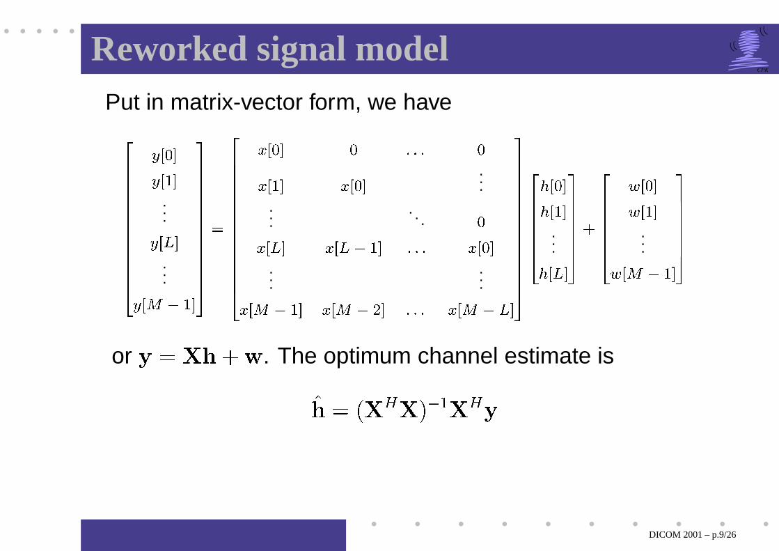
Reworked signal modelPut in matrix-vector form, we have

[\�\]\�\]\�\�\]\�\^\^\^\�\`_M Ia K

M I � K

...M Ib K

...M Ic d � Kef�f]f�f]f�f�f]f�f^f^f^f�f`g

h[\^\^\^\^\�\]\�\^\^\^\�\]\�\`_HIa K a i i i a

HI� K HIa K ......

. . . a

HIb K HI b d � K i i i HIa K...

...HIc d � K HIc d j K i i i HIc d b Kef^f^f^f^f�f]f�f^f^f^f�f]f�f`g

[\�\]\�\^\^\`_L Ia KL I� K

...L Ib Kef�f]f�f^f^f`g

k[\�\]\�\^\^\`_N Ia K

N I� K

...N I c d � Kef�f]f�f^f^f`g

or � � l m � �. The optimum channel estimate is

� m � + l & l , d � l & �

DICOM 2001– p.9/26

Example: Measured UMTS channelWe have a measured impulse response:

1 2 3 4 5 6 7−1

−0.5

0

0.5

1real part of channel

1 2 3 4 5 6 7−1

−0.5

0

0.5

1imaginary part of channel

We have

npo q

and we choose

rpo s t

. The SNR is 20dB.

DICOM 2001– p.10/26

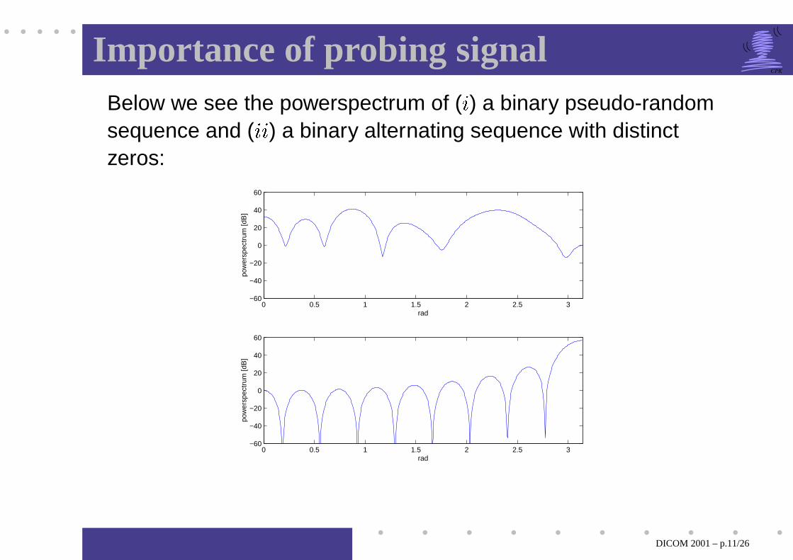
Importance of probing signalBelow we see the powerspectrum of (

u

) a binary pseudo-randomsequence and (

u u

) a binary alternating sequence with distinctzeros:

0 0.5 1 1.5 2 2.5 3−60

−40

−20

0

20

40

60

rad

pow

ersp

ectr

um [d

B]

0 0.5 1 1.5 2 2.5 3−60

−40

−20

0

20

40

60

rad

pow

ersp

ectr

um [d

B]

DICOM 2001– p.11/26

The estimated impulse response

1 2 3 4 5 6 7−1

−0.5

0

0.5

1real part of channel

1 2 3 4 5 6 7−1

−0.5

0

0.5

1imaginary part of channel

(a) Pseudo-random probing signal

1 2 3 4 5 6 7−1

−0.5

0

0.5

1real part of channel

1 2 3 4 5 6 7−1

−0.5

0

0.5

1imaginary part of channel

(b) Alternating probing signal

We see a clear advantage of using a pseudo-random prob-

ing signal.

DICOM 2001– p.12/26

Applications to deconvolution

DICOM 2001– p.13/26

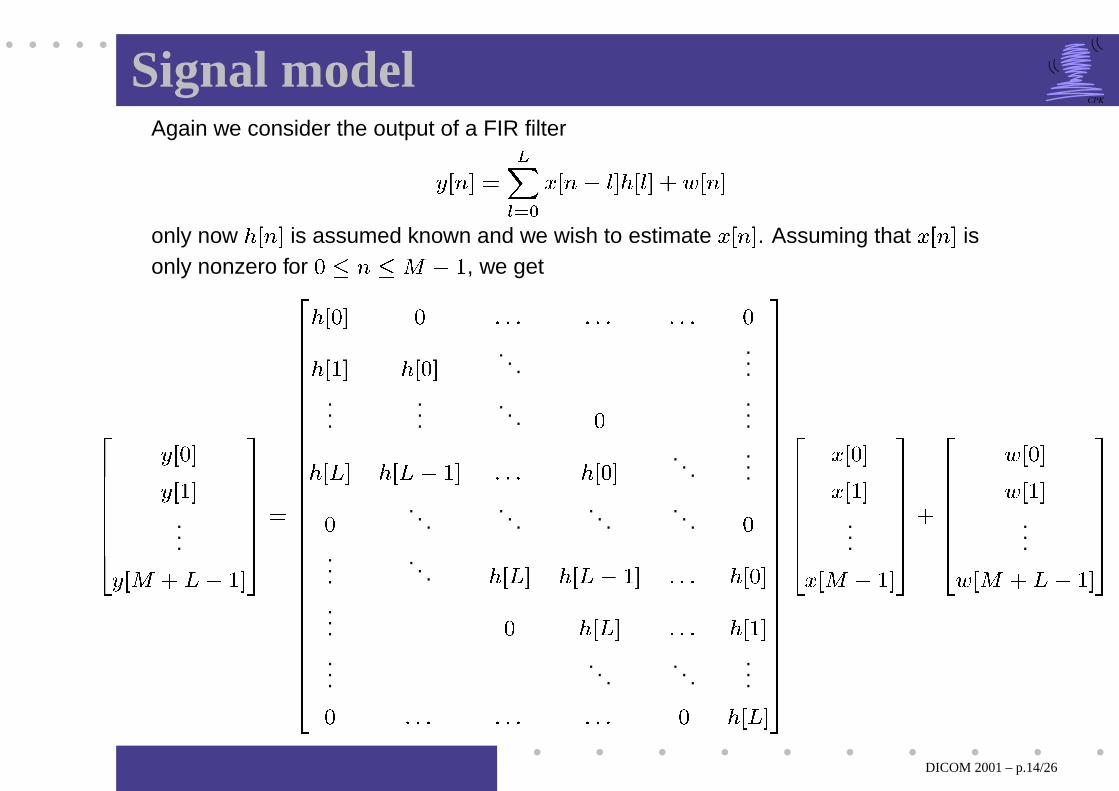
Signal modelAgain we consider the output of a FIR filter

M IJ" K h vwyx z HIJ" d { K L I { K k N IJ" K

only now

L IJ" K

is assumed known and we wish to estimate HI " K

. Assuming that HI " Kis

only nonzero for

a| " | c d � , we get

[\^\^\^\�\]\`_M Ia K

M I� K

...M I c k b d � Kef^f^f^f�f]f`g

h[\�\^\^\^\�\]\�\�\]\�\]\�\^\^\^\�\]\�\^\^\^\�\]\�\�\]\`_L Ia K a i i i i i i i i i a

L I � K L Ia K . . ....

......

. . . a ...L Ib K L Ib d � K i i i L Ia K . . ....a . . .

. . .. . .

. . . a

.... . .

L Ib K L Ib d � K i i i L Ia K

...a L Ib K i i i L I� K

.... . .

. . ....a i i i i i i i i i a L Ib K

ef�f^f^f^f�f]f�f�f]f�f]f�f^f^f^f�f]f�f^f^f^f�f]f�f�f]f`g[\^\^\^\�\]\`_HIa K

HI� K

...HI c d � Kef^f^f^f�f]f`g

k[\^\^\^\�\]\`_N Ia K

N I� K

...N Ic k b d � Kef^f^f^f�f]f`g

DICOM 2001– p.14/26

Zero-forcing equalizerAs before the estimate of } is~ }o �� & � � d � � &����

This is the optimal solution to~ }o �� � � ����� � � � � � � } � ji.e. without restrictions on }.However, if } � � � s�� � s � c

the problem is much harder to solve.

A suboptimal solution to this problem is

� o � � & � � d � � &��

~��� o � � �� ��   �¢¡ � � �� u o £�� � � � r � s

This solutions is called the Zero-forcing equalizer, as it forces the

ISI to zero. The draw-back is a degradation of the SNR.

DICOM 2001– p.15/26

Ex: equalization of UMTS channelWe use the measured UMTS channel for a burst of

ro s £ £bits. We assume that the channel is perfectly known.

−2 −1 0 1 2−2

−1

0

1

2

real part

imag

inar

y pa

rt

SNR=10dB

−2 −1 0 1 2−2

−1

0

1

2

real part

imag

inar

y pa

rt

SNR=20dB

−2 −1 0 1 2−2

−1

0

1

2

real part

imag

inar

y pa

rt

SNR=30dB

−2 −1 0 1 2−2

−1

0

1

2

real part

imag

inar

y pa

rt

SNR=40dB

DICOM 2001– p.16/26

Array application

DICOM 2001– p.17/26

Array applicationRecall the array model from lecture 1

+ ++...

¤¥ ¦ §A¨ ¥ ©ª« ¬­J® ¯±° ¤¥ ²³µ´²³ ´·¶ ¸ ° ¤¥ ¦ ¹® §A¨ °

­J®

º»½¼ ¾ ¿AÀ Á

 ¾ ¿AÀ Á Âà ¿AÀ Á

¦ ¹®º ¾ ¿AÀ Á

¦Â»½¼ ¾ ¿AÀ Á

º Ã ¿ À Á

Lineararray

Planewaveswih incidentangle:

­Ä®

Omnidirectionalantenna

Equidistance:

¦Å Æ�Ç ´ÈÉ

¦ ¹® ° ¦ ©ª« ¬­® ¯Ê® ¿AÀ ÁAË ® ¿ À Á

DICOM 2001– p.18/26

Array applicationWe have 4 equal powered users with 4 distinct electrical angles

0.2

0.4

0.6

0.8

1

30

210

60

240

90

270

120

300

150

330

180 0

We now want to use the ZF spatial equalizer to estimate the sig-

nals from the 4 users.

DICOM 2001– p.19/26

Array applicationThe array manifold of the ZF exhibits nulls at “interferers”

irrespective of the noise level -> Nulling beamformer.

−2 0 2−40

−30

−20

−10

0

10

20Array manifold for user 1

Pow

er [d

B]

−2 0 2−40

−30

−20

−10

0

10

20Array manifold for user 2

Pow

er [d

B]

−2 0 2−40

−30

−20

−10

0

10

20Array manifold for user 3

Pow

er [d

B]

−2 0 2−40

−30

−20

−10

0

10

20Array manifold for user 4

Pow

er [d

B]

DICOM 2001– p.20/26

Array applicationScatterplots at SNR=15db (blue) and SNR=25dB (red).

−2 −1 0 1 2−2

−1

0

1

2

Inphase

Qua

drat

ure

−2 −1 0 1 2−2

−1

0

1

2

Inphase

Qua

drat

ure

−2 −1 0 1 2−2

−1

0

1

2

Inphase

Qua

drat

ure

−2 −1 0 1 2−2

−1

0

1

2

Inphase

Qua

drat

ure

DICOM 2001– p.21/26

Extensions of model to coloured noise

DICOM 2001– p.22/26

Coloured noiseIn the linear model

� � ��� �ÍÌ

we made the important assumption that Ì is whiteGaussian noise, i.e. that

Î PÌ Ì - Q � = � � +ÐÏ �3 ! ! ! Ï � D ,

If instead Ì is coloured Gaussian with covarianceÎ P � � - Q � Ñ

for an arbitrary Hermitian

Ñ

, we factor it as

Ñ � Ò Ò -

e.g. with a Cholesky factorization.

DICOM 2001– p.23/26

Coloured noiseWe next transform the signal model as

Ó � Ò1 3 � � Ô � � � �The covariance of the filtered noise is

Î P � � - Q � Ò1 3 Î PÌ Ì - Q Ò1 - � Õ

Thus the noise in the modified signal model is white, andthe results from before now apply.

It can be shown, that the LS solution for the modifiedmodel using a whitening transformation is still optimal.

DICOM 2001– p.24/26

Summary of lecture

DICOM 2001– p.25/26

SummaryIn this lecture we have seen:

How to obtain the LS solution to � � � � � � incomplex form.

That this solution is optimal when � is “analogous”.

How it is related to the pseudo-inverse solution.

How to apply this solution tochannel estimation.zero-forcing equalization.nulling beamforming.

DICOM 2001– p.26/26