Array Signal Processing - OpenStax CNX · Chapter 1 Array Signal Processing: An Introduction 1 1.1 Introduction and Abstract Array signal processing is a part of signal processing

Array Signal Processing

By:Jeremy Bass

Claiborne McPheetersJames Finnigan

Edward Rodriguez

Array Signal Processing

By:Jeremy Bass

Claiborne McPheetersJames Finnigan

Edward Rodriguez

Online:< http://cnx.org/content/col10255/1.4/ >

C O N N E X I O N S

Rice University, Houston, Texas

This selection and arrangement of content as a collection is copyrighted by Jeremy Bass, Claiborne McPheeters, James

Finnigan, Edward Rodriguez. It is licensed under the Creative Commons Attribution 2.0 license (http://creativecommons.org/licenses/by/2.0/).

Collection structure revised: July 20, 2005

PDF generated: October 25, 2012

For copyright and attribution information for the modules contained in this collection, see p. 52.

Table of Contents

1 Array Signal Processing: An Introduction . . . . . . . . . . . . . . . . . . . . . . . . . . . . . . . . . . . . . . . . . . . . . . . . . . . . . . 12 Beamforming Basics . . . . . . . . . . . . . . . . . . . . . . . . . . . . . . . . . . . . . . . . . . . . . . . . . . . . . . . . . . . . . . . . . . . . . . . . . . . . . . 53 Developing the Array Model and Processing Techniques . . . . . . . . . . . . . . . . . . . . . . . . . . . . . . . . . . . . . 94 Spatial Frequency . . . . . . . . . . . . . . . . . . . . . . . . . . . . . . . . . . . . . . . . . . . . . . . . . . . . . . . . . . . . . . . . . . . . . . . . . . . . . . . . 135 Spatial Frequency Analysis . . . . . . . . . . . . . . . . . . . . . . . . . . . . . . . . . . . . . . . . . . . . . . . . . . . . . . . . . . . . . . . . . . . . . . 156 Labview Implementation . . . . . . . . . . . . . . . . . . . . . . . . . . . . . . . . . . . . . . . . . . . . . . . . . . . . . . . . . . . . . . . . . . . . . . . . 197 Microphone Array Simulation . . . . . . . . . . . . . . . . . . . . . . . . . . . . . . . . . . . . . . . . . . . . . . . . . . . . . . . . . . . . . . . . . . 318 Hardware . . . . . . . . . . . . . . . . . . . . . . . . . . . . . . . . . . . . . . . . . . . . . . . . . . . . . . . . . . . . . . . . . . . . . . . . . . . . . . . . . . . . . . . . . 379 Limitations to Delay and Sum Beamformers . . . . . . . . . . . . . . . . . . . . . . . . . . . . . . . . . . . . . . . . . . . . . . . . . . 3910 Results . . . . . . . . . . . . . . . . . . . . . . . . . . . . . . . . . . . . . . . . . . . . . . . . . . . . . . . . . . . . . . . . . . . . . . . . . . . . . . . . . . . . . . . . . . . 4111 The Team . . . . . . . . . . . . . . . . . . . . . . . . . . . . . . . . . . . . . . . . . . . . . . . . . . . . . . . . . . . . . . . . . . . . . . . . . . . . . . . . . . . . . . . . 45Glossary . . . . . . . . . . . . . . . . . . . . . . . . . . . . . . . . . . . . . . . . . . . . . . . . . . . . . . . . . . . . . . . . . . . . . . . . . . . . . . . . . . . . . . . . . . . . . 50Index . . . . . . . . . . . . . . . . . . . . . . . . . . . . . . . . . . . . . . . . . . . . . . . . . . . . . . . . . . . . . . . . . . . . . . . . . . . . . . . . . . . . . . . . . . . . . . . . 51Attributions . . . . . . . . . . . . . . . . . . . . . . . . . . . . . . . . . . . . . . . . . . . . . . . . . . . . . . . . . . . . . . . . . . . . . . . . . . . . . . . . . . . . . . . . . 52

iv

Available for free at Connexions <http://cnx.org/content/col10255/1.4>

Chapter 1

Array Signal Processing: An

Introduction1

1.1 Introduction and Abstract

Array signal processing is a part of signal processing that uses sensors that are organized in patterns, orarrays, to detect signals and to determine information about them. The most common applications ofarray signal processing involve detecting acoustic signals, which our project investigates. The sensors inthis case are microphones and, as you can imagine, there are many ways to arrange the microphones. Eacharrangement has advantages and drawbacks based on what it enables the user to learn about signals thatthe array detects. We began the project with the goal of using an array to listen to relatively low frequencysounds (0 to 8 kHz) from a specic direction while attenuating all sound not from the direction of interest.Our project demonstrates that the goal, though outside the capabilities of our equipment, is achievable andthat it has many valuable applications.

Our project uses a simple but fundamental design. We created a six-element uniform linear array, or(ULA), in order to determine the direction of the source of specic frequency sounds and to listen to suchsounds in certain directions while blocking them in other directions. Because the ULA is one dimensional,there is a surface of ambiguity on which it is unable to determine information about signals. For example,it suers from 'front-back ambiguity,' meaning that signals incident from 'mirror locations' at equal angleson the front and back sides of the array are undistinguishable. Without a second dimension, the ULA isalso unable to determine how far away a signal's source is or how high above or below the array's level thesource is.

1This content is available online at <http://cnx.org/content/m12561/1.6/>.


1

2 CHAPTER 1. ARRAY SIGNAL PROCESSING: AN INTRODUCTION

Uniform Linear Array

Figure 1.1: The ULA is the simplest array design, though it has limitations.

When constructing any array, the design specications should be determined by the properties of thesignals that the array will detect. All acoustic waves travel at the speed of sound, which at standardtemperature and pressure of 0 degrees celsius and 1 atm, is dened as :

c ≡ 330.7m

s(1.1)

The physical relationship describing acoustic waves is similar to that of light: λf = c. The frequenciesof signals that an array detects are important because they determine constraints on the spacing of thesensors. The array's sensors sample incident signals in space and, just as aliasing occurs in analog to digitalconversion when the sampling rate does not meet the Nyquist criterion, aliasing can also happen in space ifthe sensors are not suciently close together.

A useful property of the ULA is that the delay from one sensor to the next is uniform across the arraybecause of their equidistant spacing. Trigonometry reveals that the additional distance the incident signaltravels between sensors is dsin (θ) . Thus, the time delay between consecutive sensors is given by:

τ =d

csin (θ) (1.2)

Say the highest narrowband frequency we are interested is fmax . To avoid spatial aliasing, we would liketo limit phase dierences between spatially sampled signals to π or less because phase dierences above πcause incorrect time delays to be seen between received signals. Thus, we give the following condition:

2πτ fmax ≤ π (1.3)


3

Substituting for τ in (2), we get

d ≤ c

2fmaxsin (θ)(1.4)

The worst delay occurs for θ = 90 , so we obtain the fundamentally important condition

d ≤ λmin

2(1.5)

for the distance between sensors to avoid signals aliasing in space, where we have simply used λmin = cfmax

.

We refer to the direction perpendicular to the length of the array as the broadside of the array.All angles to the right, or clockwise from the broadside are considered positive by convention up to+90 . All angles to the left, or counter-clockwise from the broadside are considered negative up to−90 .

Just think of spatial sampling in a similar sense as temporal sampling: the closer sensors are, the moresamples per unit distance are taken, analogous to a high sampling rate in time!


4 CHAPTER 1. ARRAY SIGNAL PROCESSING: AN INTRODUCTION

Ambiguity of the ULA

Figure 1.2: The ULA is unable to distinguish signals from it's front or back side, or signals above orbelow it.

The limitations of the ULA obviously create problems for locating acoustic sources with much accuracy.The array's design is highly extensible, however, and it is an important building block for more complexarrays such as a cube, which uses multiple linear arrays, or more exotic shapes such as a circle. We aimmerely to demonstrate the potential that arrays have for acoustic signal processing.


Chapter 2

Beamforming Basics1

2.1 Introduction to Beamforming

Beamformer BasicsBeamforming is just what the name sounds like, no pun intended. Beamforming is the process of trying toconcentrate the array to sounds coming from only one particular direction. Spatially, this would look like alarge dumbbell shaped lobe aimed in the direction of interest. Making a beamformer is crucial to meet oneof the goals of our project, which is to listen to sounds in one direction and ignore sounds in other directions.The gure below, while it accentuates what we actually accomplished in Labview, it illustrates well what wewant to do. The best way to not listen in 'noisy' directions, is to just steer all your energy towards listeningin one direction. This is an important concept, because it is not just used for array signal processing, it isalso used in many sonar systems as well. RADAR is actually the complete opposite process, so we will notdeal with that.



5

6 CHAPTER 2. BEAMFORMING BASICS

Figure 2.1: Visualization of a Beamformer

Delay & Sum BeamformersEven though we did not use a delay and sum beamformer for the implementation of our project, it is a goodrst step to discuss, because it is the simplest example. While, we were doing research for this project oneof the rst beamformers we learned about was the delay and sum beamformer because of its simplicity. Thedelay and sum beamformer is based on the idea that if a ULA is being used, then the output of each sensorwill be the same, except that each one will be delayed by a dierent amount. So, if the output of each sensoris delayed appropriately then we add all the outputs together the signal that was propagating through thearray will reinforce, while noise will tend to cancel. In the Introductory module, we discussed what the timedelay is for a linear array, so since the delay can be found easily, we can delay each sensor appropriately.This would be done by delaying the rst sensor output by nτ , where n is the sensor number after the rst.A block diagram of this can be seen below.

Figure 2.2: Block Diagram for a Delay & Sum Beamformer

Does this Really Work?This seems too simple and to easy to work in practice. Delay and sum beamformers are not very commonlyused in practical applications, because they do not work to well, but they do explain a tricky concept simply,


7

which is why they are often used to introduce beamforming. The problem with further development oftime-domain beamformers, such as the delay and sum is that time-domain beamformers are often dicultto design. It is often easier to look at the frequency domain to design lters, which we can then use to steerthe attention our array. However, this is no ordinary frequency analysis, this is Spatial Frequency!2

2http://cnx.rice.edu/content/m12564/latest/


8 CHAPTER 2. BEAMFORMING BASICS


Chapter 3

Developing the Array Model and

Processing Techniques1

We continue to develop the properties for the uniform linear array (ULA) that has been discussed previously2

. With the important relationship that we found to avoid spatial aliasing, d ≤ λmin2 , we now consider the

theoretical background of the ULA. Once we understand how the array will be used, we will look at a methodcalled 'beamforming' that directs the array's focus in specic directions.

3.1 Far-eld Signals

We saw previously that a very nice property of the ULA is the constant delay between the arrival of asignal at consecutive sensors. This is only true, however, if we assume that plane waves arrive at the array.Remember that sounds radiate spherically outward from their sources, so the assumption is generally nottrue! To get around that problem, we only consider signals in the far-eld, in which case the signal sourcesare far enough away that the arriving sound waves are essentially planes over the length of the array.

Denition 3.1: Far-eld sourceA source is considered to be in the far-eld if r > 2L2

λ , where r is the distance from the source tothe array, L is the length of the array, and λ is the wavelength of the arriving wave.

If you have an array and sound sources, you can tell whether the sources are in the far-eld based onwhat angle the array estimates for the source direction compared to the actual source direction. If the sourceis kept at the same angle with respect to the broadside and moved further away from the array, the estimateof the source direction should improve as the arriving waves become more planar. Of course, this only worksif the array is able to accurately estimate far-eld source directions to begin with, so use the formula rst tomake sure that everything works well in the far-eld, and then move closer to see how distance aects thearray's performance.

Near-eld sources are beyond the scope of our project, but they are not beyond the scope of arrayprocessing. For more information on just about everything related to array processing, take a look at ArraySignal Processing: Concepts and Techniques, by Don H. Johnson and Dan E. Dudgeon, EnglewoodClis, NJ: Prentice Hall, 1993.

1This content is available online at <http://cnx.org/content/m12562/1.3/>.2http://cnx.rice.edu/content/m12561/latest/


9

10CHAPTER 3. DEVELOPING THE ARRAY MODEL AND PROCESSING

TECHNIQUES

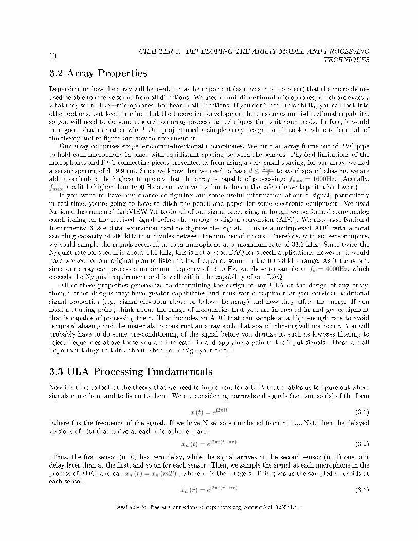
3.2 Array Properties

Depending on how the array will be used, it may be important (as it was in our project) that the microphonesused be able to receive sound from all directions. We used omni-directional microphones, which are exactlywhat they sound like microphones that hear in all directions. If you don't need this ability, you can look intoother options, but keep in mind that the theoretical development here assumes omni-directional capability,so you will need to do some research on array processing techniques that suit your needs. In fact, it wouldbe a good idea no matter what! Our project used a simple array design, but it took a while to learn all ofthe theory and to gure out how to implement it.

Our array comprises six generic omni-directional microphones. We built an array frame out of PVC pipeto hold each microphone in place with equidistant spacing between the sensors. Physical limitations of themicrophones and PVC connecting pieces prevented us from using a very small spacing; for our array, we hada sensor spacing of d=9.9 cm. Since we know that we need to have d ≤ λmin

2 to avoid spatial aliasing, we areable to calculate the highest frequency that the array is capable of processing: fmax = 1600Hz. (Actually,fmax is a little higher than 1600 Hz as you can verify, but to be on the safe side we kept it a bit lower.)

If you want to have any chance of guring out some useful information about a signal, particularlyin real-time, you're going to have to ditch the pencil and paper for some electronic equipment. We usedNational Instruments' LabVIEW 7.1 to do all of our signal processing, although we performed some analogconditioning on the received signal before the analog to digital conversion (ADC). We also used NationalInstruments' 6024e data acquisition card to digitize the signal. This is a multiplexed ADC with a totalsampling capacity of 200 kHz that divides between the number of inputs. Therefore, with six sensor inputs,we could sample the signals received at each microphone at a maximum rate of 33.3 kHz. Since twice theNyquist rate for speech is about 44.1 kHz, this is not a good DAQ for speech applications; however, it wouldhave worked for our original plan to listen to low frequency sound in the 0 to 8 kHz range. As it turns out,since our array can process a maximum frequency of 1600 Hz, we chose to sample at fs = 4000Hz, whichexceeds the Nyquist requirement and is well within the capability of our DAQ.

All of these properties generealize to determining the design of any ULA or the design of any array,though other designs may have greater capabilities and thus would require that you consider additionalsignal properties (e.g., signal elevation above or below the array) and how they aect the array. If youneed a starting point, think about the range of frequencies that you are interested in and get equipmentthat is capable of processing them. That includes an ADC that can sample at a high enough rate to avoidtemporal aliasing and the materials to construct an array such that spatial aliasing will not occur. You willprobably have to do some pre-conditioning of the signal before you digitize it, such as lowpass ltering toreject frequencies above those you are interested in and applying a gain to the input signals. These are allimportant things to think about when you design your array!

3.3 ULA Processing Fundamentals

Now it's time to look at the theory that we need to implement for a ULA that enables us to gure out wheresignals come from and to listen to them. We are considering narrowband signals (i.e., sinusoids) of the form

x (t) = ej2πft (3.1)

where f is the frequency of the signal. If we have N sensors numbered from n=0,...,N-1, then the delayedversions of x(t) that arrive at each microphone n are

xn (t) = ej2πf(t−nτ) (3.2)

Thus, the rst sensor (n=0) has zero delay, while the signal arrives at the second sensor (n=1) one unitdelay later than at the rst, and so on for each sensor. Then, we sample the signal at each microphone in theprocess of ADC, and call xn (r) = xn (mT ) , where m is the integers. This gives us the sampled sinusoids ateach sensor:

xn (r) = ej2πf(r−nτ) (3.3)


11

Now we need to do some Fourier transforms to look at the frequency content of our received signals.Even though each sensor receives the same frequency signal, recall that delays x (t− nτ) in time correspondto modulation by e−jnτ in frequency, so the spectra of the received signals at each sensor are not identical.The rst Discrete Fourier Transform (DFT) looks at the temporal frequency content at each sensor:

Xn (k) =1√R

R−1∑r=0

ej2πf(r−nτ)e−j2πkrR (3.4)

e−j2πfnτ

√R

(3.5)

for k=fn, and zero otherwise. Here we have used the denition of the normalized DFT, but it isn't partic-ularly important whether you use the normalized or unnormalized DFT because ultimately the transformfactors 1/Sqrt(R) or 1/R just scale the frequency coecients by a small amount.

Now that we have N spectra from each of the array's sensors, we are interested to see how a certainfrequency of interest fo is distributed spatially. In other words, this spatial Fourier transform will tellus how strong the frequency fo for dierent angles with respect to the array's broadside. We perform thisDFT by taking the frequency component from each received signal that corresponds to fo and concatenatingthem into an array. We then zero pad that array to a length that is a power of two in order to make the FastFourier Transform (FFT) computationally ecient. (Every DFT that we do in this project is implementedas an FFT. We use the DFT in developing the theory because it applies always, whereas the FFT is onlyfor computers.)

note: When we build the array of frequency components from each of the received signals, we havean N length array before we zero pad it. Let's think about the resolution of the array, which refersto its ability to discriminate between sounds coming from dierent angles. The greater the numberof sensors in the array, the ner the array's resolution. Therefore, what happens when we zero padthe array of frequency components? We are essentially adding components from additional 'virtualsensors' that have zero magnitude. The result is that we have improved resolution! What eectdoes this have? Read on a bit!.

Once we have assembled our zero padded array of components fo, we can perform the spatial DFT:

Ω (k) =1√NR

N−1∑n=0

e−j2π( kN+f0τ) (3.6)

where N for this equation is the length of the zero padded array and R remains from the temporal DFT.The result of the summation is a spectrum that is a digital sinc function centered at f0τ . The value of thesinc represents the magnitude of the frequency fo at an angle theta. Because of the shape of the lobes ofthe sinc, which look like beams at the various angles, the process of using the array to look for signals indierent directions is called beamforming. This technique is used frequently in array processing and it iswhat enabled us to detect the directions from which certain frequency sounds come from and to listen indierent directions.

Recalling that we zero padded our array of coecients corresponding to f0, what has that done for usin terms of the spatial spectrum? Well, we have improved our resolution, which means that the spectrumis smoother and more well-dened. This is because we are able to see the frequency dierences for smallerangles. If we increase the actual number of sensors in the array, we will also improve our resolution andwe will improve the beamforming by increasing the magnitude of the main lobe in the sinc spectrum anddecreasing the magnitudes of the side lobes.


12CHAPTER 3. DEVELOPING THE ARRAY MODEL AND PROCESSING

TECHNIQUES


Chapter 4

Spatial Frequency1

4.1 Temporal Frequency

Problems with Temporal Frequency AnalysisWe are accustomed to measuring frequency in terms of (1/seconds), or Hz. Sometimes we may even measurefrequency in rad/sec, which is often called angular frequency. More information about temporal frequencycan be found here2 . The reason we often use frequency domain techniques is because it allows for ltering3

of noise and various signals. If were just interested in listening to a particular tone, say a 500 Hz sine wave,it would be easy to just tune in to that one frequency, we would just bandpass lter out all the other noise.However, when we do this we get no information about where the signal is coming from. So, even thoughwe could easily ignore noise, we could not steer our array to just listen in one direction. It would be morelike giving it 'selective hearing.' It hears what it wants to, which in this case would be signals at 500 Hz.

4.2 Propagating Waves

Nature of WavesAs Dr. Wilson discusses in his modules4 on waves propagating down a transmission line, waves carry twoforms information in two domains. These domains are the time and space domains, because the wave equationis usually written in terms of s(x,t) because it propagates in space at a particular time, and if one looks atstanding wave at a particular point in space, one should notice that it still moves up and down in a similarmanner. An example of this illustrated below. So, if we only look at the temporal frequency component, weare missing out on half the information being transmitted in the propagating signal! If we really want to beable to steer our array in a direction, then we need to analyze the spatial frequency components.

1This content is available online at <http://cnx.org/content/m12564/1.4/>.2http://cnx.rice.edu/content/m0038/latest/3http://cnx.rice.edu/content/m0533/latest/4http://cnx.rice.edu/content/m10095/latest


13

14 CHAPTER 4. SPATIAL FREQUENCY

Figure 4.1: Illustration of a wave propagating in space

4.3 Spatial Frequency

Introduction to Spatial FrequencyWhile we were investigating the time domain, we were able to accomplish such operations as ltering bytaking 2π / T , where T is the period of the signal, to get the temporal frequency denotated ω. We can usesimilar reasoning to obtain k, the wavenumber, which is the measure of spatial frequency. Instead of usingthe period of the signal, we now use the wavelength, which is the spatial equivalent to the period. Thismakes sense, because a period is the length of time it takes to complete one cycle, whereas the wavelengthis the amount of distance the wave covers in one cycle. We there are able to change the temporal frequencyequation ω = 2π / T into k = 2π / λ.


Chapter 5

Spatial Frequency Analysis1

5.1 Aliasing in the Spatial Frequency Domain

Avoiding Spatial AliasingAs we saw was the case in the time domain, a phenomenon known as aliasing2 can occur in the frequencydomain if signals are not sampled at high enough rate. We have the same sort of considerations to takeinto account when we want to analyze the spectrum of the spatial frequency as well. As was discussed inthe introduction3 , the Nyquest equivalent of the sampling rate is 1/2 of the minimum wavelength. Thiscomes about from the relationship between speed, frequency and wavelength, which was discussed in theintroduction as well. The gure below demonstrates the eects of aliasing in the spatial domain; it looksidentical to ltering the time domain except that instead of the x-axis being related to pi/T it is now pi/d,where d is the distance between sensors. So, if we bandlimit our signal in temporal frequency, so that wecan sample as two times the maximum temporal frequency, and if we design the sensors so that half ofthe minimum wavelength is greater than distance between sensors, we can avoid aliasing in both time andspace!

Figure 5.1: Spatial Aliasing

1This content is available online at <http://cnx.org/content/m12557/1.5/>.2http://cnx.rice.edu/content/m10793/latest/3http://cnx.rice.edu/content/m12561/latest/


15

16 CHAPTER 5. SPATIAL FREQUENCY ANALYSIS

5.2 Spatial Frequency Transform

Introduction to the Spatial Frequency TransformAnalogous to the DFT4 , is the sampled and windowed spatial equivalent, which is what we used to be ableto lter our signal in frequency. The reason we want the information in the spatial frequency or wavenumberdomain is because it is directly correlated to the angle the signal is coming from relative to the ULA. Thespatial DFT is computed as the FFT of the rst FFT. The rst FFT represents the time domain frequencyresponse and the second FFT represents the wavenumber response. This seems strange this would work, butlet's explore this a little more fully. Let's look at theoretical example.

Example 5.1: Mentally Visualizing the Spatial Frequency TransformThe 2-D TransformConsider a box lled with numbers. The box is labeled on one edge time and on the other edge space.The rst FFT we are taking is to obtain the temporal frequencies, so this would be like looking ata row along the box and taking the FFT of the numbers going across, while the spatial FFT wouldbe calculated by looking at the numbers going down the columns. This is done repeatedly on eachrow and column, so the rst FFT would go across each row, while the 2nd one would go down eachcolumn. This is easier to comprehend with a picture like the one below.

4http://cnx.rice.edu/content/m10249/latest/


17

Figure 5.2: Visualization of mapping a signal into Spatial & Temporal Frequencies

SFT with SinusoidsSince we were interested in detecting sinusoids, it would be interesting to consider what this kind of "double"Fourier Transform would do to a sinusoid. From our list of Fourier Transforms5 we know that the FFT ofa sinusoid will give us a delta function shifted by the frequency of the sinusoid. We then see that the FFTof a delta function is 1, which would mean that we get the equivalent of white noise in spatial frequency!Fortunately, this is not exactly how the spatial FFT works. We are basically taking the FFT across one setof vectors followed by the FFT down the columns of those vectors, we are NOT taking the FFT(FFT(f(x,t)).So, when we accomplish this sort of arrangement on our signal, f(x,t), we get:

5http://cnx.rice.edu/content/m10099/latest


18 CHAPTER 5. SPATIAL FREQUENCY ANALYSIS

Figure 5.3: Spatial FFT of a Sinusoid

A sinc function!

5.3 Spatial Domain Filtering

Just as we are able to lter signals in temporal frequency, we can lter signals in spatial frequency. Infact, the way we accomplished the direction detecting algorithm in labview used a graph very similiar as theone above and then looking for the largest magnitude part of the signal. Once, this value is known, quickcomputation can then nd the angle that signal came from! Ta da! We're done! Well, sort of.


Chapter 6

Labview Implementation1



19

20 CHAPTER 6. LABVIEW IMPLEMENTATION

6.1 Labview VIs Used in Simulation

Top Level Diagram and Overall OrganizationThe gure below is a top level diagram of a six microphone array simulation VI. This VI is named "MultipleFrequency Simulation" Starting at the left with the signal generation, the code ows to the right. This topVI is made out of smaller VIs that each perform a specic function. Detailed descriptions of each of thesecan be found in the following paragraphs.

Top Level Diagram (Multiple Frequency Simulation)

Figure 6.1: Top Level Diagram


21

6.2 Simulated Signal Generation VI

Simulate Signal Icon

Figure 6.2: Simulate Signal Icon

Signal Generation VIThe above icon corresponds to the Signal Generation VI. At the far left are four signal generation VIs. Eachof these VIs produces six dierent signals that simulate the delayed signals that each of the microphoneswould hear in real life. These six signals are then bunched together in a cluster (pink wire) to keep theamount of wires down. The three inputs to this VI are the frequency of the sinusoid desired, the direction ofthe signal, and the distnace between microphones (9.9 cm in this example). The user sets these paramaterson the front panel and is free to change them at any time.

Our VI uses the formula discussed in previous modules that relates the time delay of signals to thedistance between microphones. Using the desired angle that the signal is coming from, the speed of sound(C), the distance between microphones, and a conversion between degrees and radians, the VI rst computesthe time delay between microphones. Becuase we are interested in the delay between the rst microphoneand all others, the amount of delay is multiplied by zero for the rst mic, one for the second mic, two forthe third, and so on. These delays are then used as phase inputs to the six identical Simulate Signal VIs.Adding phase to a periodic signal like the sinusoids being used here has the same eect as delaying the signalin time. Finally the six signals are merged together into a cluster so that they will be easier to deal with asa group in other VIs.



Simulate Signal Block Diagram

Figure 6.3: Simulate Signal Block Diagram

In this simulation we simulate four dierent frequencies and directions. Once we have the data of thesefour separate signals, we sum the signals on each of the channels to get the nal output on each of themicrophones. Doing so leaves us solely with what we would hear on the six microphones if this were set upin real life. If more signals are required for future testing or other applications, onc can simply copy andpaste the signal generation VI and then sum it with the other signals.

Once this signal is comple, we move to the right in our VI. From here we branch into two separate areas.Following the pink line up takes us to where we calculate the angle that a given frequency is coming from,andto the right is where we perform the calculations to listen to signals from a given direction.


23

6.3 Frequency and Spatial FFT Computation VIs

1rst FFT Icon (Time - Frequency)

Figure 6.4: 1rst FFT Icon

1rst FFT VIIn order to listen to a certain direction we rst need to transform our signals from the microphone in tothe frequency domain. To do this we made the "1rst FFT" Vi (see icon above). This sub-VI is fairly simpleso there is no need to show the block diagram. It takes the FFT of each of the six channels channels,transfroming the data from the time domain to the freqeuncy domain For simulation, we looked at 1 secondsamples at 4000hz. This VI then takes the FFTs of the six 4000 element long signals from the simulatedmicrophones.



Six Point FFT Icon (Frequency - Spatial)

Figure 6.5: Six Point FFT Icon(Frequency - Spatial)

Six Point FFT VIMoving to the right after the rst FFT, we nd the "6 pt FFT" VI. This VI is used to transform ourfrequency domain data into the spatial domain. This VI needs to run for every frequency of interest, so inthe top level diagram this VI is found inside of a for loop. The user can control what range of frequenciesare of interest on the front panel of the main VI, and the loop will run for those frequencies.

Inside this VI, the complex frequency coecient for the given frequency is extracted from the array foreach microphone channel. These six values are then concantonated into a lengh six array. Next, the array iszeropadded to a user specied length (we used 256 in our simulation) so more resolution can be observed inthe resulting spatial transform. Finally, the FFT is performed on these values transforming them into thespatial domain. With the data in the spatial domain we are easily able to gure out the magnitude of anyfrequency from any direction in our 180 degrees of interest. How to do this can be found in the magnitudeVI.


25

Six Point FFT block Diagram (Frequency - Spatial)

Figure 6.6: Six Point FFT block Diagram (Frequency - Spatial)



6.4 Coecient, Angle, and Magnitude Calculation VIs

Coecient Calculator

Figure 6.7: Coecient Calculator

Coecient CalculatorNow that the signals have been transformed to their spatial representations, the correct coecients toconstruct the signal of interest must be computed. To do this we created the Coecient Calculator VI..This VI takes in the angle of interest, a frequency, the number of microphones, a constant factor (determinedby the setup of the microphones and the amount of zero padding...in this example it is -93), and our originalsampling frequency to compute the correct coecient to look at for the given angle. Once this coecient isfound, we extract the value at that coecient and append it to our ouptut array as the value at that givenfrequency. Below is the block diagram for this VI. It consists of a basic formula node and some logic onthe front and back to make sure that the calculations are correct when working with angles from negativedirections.

Because this formula is dependent on the frequnecy of interest, we are required to run this VI for everyfrequency we are intereseted in. In order to do this, we put this VI inside a for loop that is controlled byour frequency range. Any coecient for frequencies outside of this range are simply given a value of zero.The array modules ouside of this for loop are used to do just that. They append arrays with value zeroon the front and back of the output of the for loop to return our vector to its original size. From here, werun this vector through a few multiplies to amplify the diernce between the coecients with high and lowmagnitudes, and nally we inverse FFT it to get our output array. This array represents a signal in thetime domain and is graphed on the front panel along with a graph of its frequency components. We alsoincluded a small VI that will play the output waveform on computer speakers. This VI uses a matlab scriptand requires the user to have matlab 6.5 or earlier.


27

Magnitude Graph of Coecients After Spatial FFT

Figure 6.8: Magnitude Graph of Coecients After Spatial FFT



Magniutde Calculation VI

Figure 6.9: Magnitude Calculation VI

Magnitude CalculationIf we go back to the branch in the pink wire immediatly after the signal generation VIs and move upwardsinstead of to the right, we come across the code that is used to calculate the angle at which the largestmagnitude signal of a given frequency is approaching the array. Another "6 pt t" VI is used, but this oneis slightly modied. It also includes the initial FFTs of all 6 channels. We grouped these two VIs togetherbecause ony one spacial FFT is being computed (that at the frequeny of interest).

The resulting vector of the previous six point FFT is immediately used as the input to the MagnitudeCalculation VI. The vecor of spatial coecients from the "six pt FFT" vis are complex, so this VI is usedto calculate the magnitudes of the coecients so the maximum coecient can be found. The output of thisVI is also used to create a visual representation of what direction the specied frequency is coming from.Below is a graph of the magnitude of the coecients of the spatial FFT. As discussed before, we see thepeak correspoinding to the incoming direction and the smaller ripples to each side.


29

Magnitude Graph of Coecients After Spatial FFT

Figure 6.10: Magniutde of Coecients after Spatial FFT

Example 6.1: Magnitude Graph ExampleAs we can see in the previous gure, the magnitude of the spatial FFT is greatest around coecient82. There are also smaller ripples that die o around each end. This graph tells us that the thedirection that the given frequency is coming from corresponds to the angle represneted by coecient82. To gure out what angle this was, we would use our Coecient to Angle VI.

Calculation of AngleFinally, we isolate the index of the maximum angle and use it to compute the angle of incidence. Usingthe same formula used in the Coecient Angle Calculator, the Coecient to Angle VI deduces the angleof incidence. This VI uses the same formula found in the Coecient Angle Calculator, but is arrangeddierently so that we can nd the angle based on the coecient instead of the coecient based on the angle.Once the VI computes this value, the result is output on the front panel.



6.4.1 Links to Labview Code

• Multiple FrequencySimulation (Top Level VI)2

• Coecient Calculator3

• Incident Angle Calculator4

• Play Array5

• Six Point FFT (with rst t)6

• Six Point FFT (without rst t)7

• Magnitude Calculation8

• First FFT9

• Simulate Signal10

6.5 Code Remarks

Overall, the code involved in this method of array signal processing can be broken up into smaller partsthat are easy to understand. By combining these smaller parts we are able to create an upper level VIthat performs a complicated task that would be dicult to get working using other methods. The majorproblem with this VI is that it requires a large number of calculations. To increase performance (withoutupgrading computers) one could decrease the frequency range of interest, or they could lower the amount ofzeropadding. They could aslo look at a smaller time period.

2http://cnx.org/content/m12565/latest/Multiple_Frequency_Simulation.vi3http://cnx.org/content/m12565/latest/Coecient_Calculator.vi4http://cnx.org/content/m12565/latest/Incident_Angle_Calculator.vi5http://cnx.org/content/m12565/latest/play_array_anything.vi6http://cnx.org/content/m12565/latest/Six_Point_FFT_with_rst_t.vi7http://cnx.org/content/m12565/latest/Six_Point_FFT_without_rst_t.vi8http://cnx.org/content/m12565/latest/Magnitude_Calculation.vi9http://cnx.org/content/m12565/latest/First_FFT.vi

10http://cnx.org/content/m12565/latest/Simulated_Input.vi


Chapter 7

Microphone Array Simulation1



31

32 CHAPTER 7. MICROPHONE ARRAY SIMULATION

7.1 Why Labview Simulation

Reasons For SimulationSimulation of the microphone array is an integral step in verifying that the design and method of imple-mentation behind the beamforming system are correct. Additionally, Simulation allows one to easily changethe paramaters of the system (number of microphones, type of signals, distance between microphones) sothat the system can be optimized to the desired needs. Simulation also allows for easy testing free of noise,uncertainty, and other errors. Finally, simulation allows one to modify input signals on the y and lets oneinstantaenously see if the system is working as planned.Reasons for Simulation in LabviewThere are many practical reasons why Labview is the ideal program to simulate array processing in. Labviewsgraphical programming environment is perfect for this type of application. The simple to use signal generatorVIs and convenient output displays make controlling the results and modifying the inputs easly. Additionally,with Labview the Simulation can be easily modied to work in real life (see next module). By replacing thesimulated signals with real life data acquiition, the same code is used for real-life implemenation of the array.

7.2 Simulation Inputs

Four independent sinusoids are used as the inputs to the simulator. Each of these sinusoids has its ownfrequency and direction of incidence. The user of the simulator can modify these signals while the VI isrunning by simply rotating the knobs or entering new values. To cut down on processing time, we decidedto bandlimit the frequencies of the sinusoids from 800 to 1600 Hz. There are other controls in the VI thatallow the user to change this range, but we found that the simulations runs most smoothly at this range.With four signals the simulator can be used to examine the major combinations of sinusoids that shouldbe tested....dierent frequencies coming from dierent directions, similar frequencies coming from dierentdirections, similar frequencies coming from the same direction, and varied frequencies coming from the samedirection. These four major categories can be used to show that the simulator does indeed work. The gurebelow shows how the paramaters of the sinusoids are input in the VI.


33

Input Signal Selection

Figure 7.1: Input Signal Selection

7.3 Simulation Front Panel

Below is a copy of the front panel of the simulation VI. The "Angle to Listen To" knob is where the userselects the direction that they want to listen to. The graph on top shows the magnitude of the variousfrequency components from the angle that they are looking at. If a user wants to know from which directiona certain frequency compnent is propogating (or if there are two signals, the one witht he greatest amplitude),they can enter that frequency on the "Desired Frequency Knob". The direction that the frequency of interestis coming from will then be displayed on the "Angle of Incidence" Meter. Overall, this Front panel alllowsthe user to listen in dierent directions and determine the direction of an incoming frequency.

Example 7.1: Simple Example Using of SimulationOn the "Front Panel" gure below, we can see that the user is listening to signals coming fromthirty degrees. We can then deduce from the graph that a signal at 1300Hz is propograting fromthirty degrees. Based on the inputs above, this is exactly what we expect to see. We can also tellfrom looking at the "Angle of Incidence" meter that a signal at 1050Hz is comign from rougly -25degrees. Again, this makes sense based on the above inputs.



FRONT PANEL

Figure 7.2: FRONT_PANEL

7.4 Simulation Output

The nal part of this Simulation VI is the ouptut. The VI will display the incoming signal coming from thedesired direction on the "Ouput Waveform" Graph. In addition to to this graph, the Simulation will alsoplay this output waveform as audio. Doing so allows the user to hear the diernt sounds as they changetheir angle of interest.


35

OUTPUT WAVEFORM

Figure 7.3: OUTPUT WAVEFORM




Chapter 8

Hardware1

8.1 Hardware

Our array was built using six Sony F-V100 omnidirectional microphones, spaced at 9.9 cm apart. We builta frame out of precisely cut 1" I.D. PVC pipe in order to keep the microphones spaced accurately apartand minimize phase error in our measurements. These microphones produced an average 1 mV p-p signalfrom the sinusoids that were used for the test program. The signals were fed into a six-channel amplier toincrease the voltage to .5 V p-p in order to achieve a usable range of the DAQ card. The amplier was builtusing common 741 op-amps and care was taken to insure all the path lengths were approximately the samelength. Following the amplier, the signals were fed into a National Instruments 6024e DAQ card. The DAQcard was set to sample at 4000 Hz for a length of 2 seconds.

8.1.1 Test Setup

Once the signals were digitized, we were able to use the Labview code that we had developed using thesimulated test signals and apply the same algorithm to the real life signals that we were recording. Togenerate test signals we used a second laptop to generate dierent frequency sinusoids on the left and rightchannel of the sound output and then used a set of speakers with extended cables to place them at dierentlocations around the array. For the actual location of the tests, we set up the array in the middle of anopen outdoor area in order to avoid sounds echoing o the walls of an enclosed space and causing unwantedinterference.



37

38 CHAPTER 8. HARDWARE


Chapter 9

Limitations to Delay and Sum

Beamformers1

9.1 Implementing a Delay and Sum Beamformer

As we discovered in the section discussing beamformers2 , that when an array of sensors record a signalthere is an implicit delay between the signal arriving at the dierent sensors because the signal has a nitevelocity and the sensors are not located at the same location in space. We can use this to our advantage, byexploiting the fact that the delay among the sensors will be dierent depending on which direction the signalis coming from, and tuning our array to "look" in a specic direction. This process is know as beamforming.The traditional way of beamforming is to calculate how much delay there will be among the sensors forsound coming from a direction that you are interested in. Once you know this delay you can delay all thecorresponding channels the correct amount and add the signals from all the channels. In this way, you willconstructively reinforce the signal that you are interested in, while signals from other directions will be outof phase and will not be reinforced.

1This content is available online at <http://cnx.org/content/m12570/1.4/>.2http://cnx.rice.edu/content/m12563/latest/


39

40 CHAPTER 9. LIMITATIONS TO DELAY AND SUM BEAMFORMERS

Figure 9.1

The gure above illustrates a sinusoid captured on a six channel linear array. Though, the sinusoids lookcrude because of the implicit noise of real signals, you can see by the spectrum that it is indeed there andin also that the phase is dierent for each of the sensors. The phase dierence is determined by the delaybetween the sensors and is given by a simple geometrical calculation which we discuss later.

The problem with this method is that the degree of resolution that you can distinguish is determined bythe sampling rate of your data, because you can not resolve delay dierences less than your sampling rate.For example if the sampling period is 3 milliseconds, then you would have a range of say 20 degrees wherethe delay would be less than 3 milliseconds, and thus they would all appear to be coming from the samedirection because digitizing signals from anywhere in this range would result in the same signal.

This is very signicant because the spacing of the sensors is usually quite small, on the order of cen-timeters. At the average rate of sound, 330 m/s, it only takes .3 milliseconds to move 10 cm. However,the Nyquist Sampling Theorem states that we can derive all the information about a signal by sampling atonly twice the highest frequency contained in the signal. With a 10 cm spacing between sensors the highestsinusoid we can capture is 1600 Hz, for reasons we discuss elsewhere. So ,we should be able determine thephase of all the sinusoids by only sampling at 3200 Hz rather than at tens of kilohertz that is requiredwith delay and sum beamforming. In order to do this, however, we must implement a better method ofbeamforming in the frequency domain.


Chapter 10

Results1

The tests of the real-world implementation were successful. Using the second laptop, we positioned a 1000Hz signal at about 40 degrees and a 1600Hz signal at about -25 degrees relative to the axis perpendicularto our array. Both signals were on simultaneously and at equal volume. As you can see from the spectrumof the output of our program, changing the dial to tune to the array to dierent directions results in theexpected behavior.

Tuned towards 40 degrees

Figure 10.1



41

42 CHAPTER 10. RESULTS

Tuned towards -25 degrees

Figure 10.2

These rst two gures show that our output signal consists of the two test sinusoids. Tuning the softwareto look in the appropriate directions shows that the magnitude of the corresponding sinusoid is more powerfulthan that of the power of the other sinusoid. Focusing on the 1000 Hz sinusoid enhances the power of thatsinusoid to about 5 times that of the other sinusoid. Focusing on the 1600 Hz sinusoid gives even betterresults. The dierence in power here is more than 10 times.


43

Tuned straight ahead

Figure 10.3


44 CHAPTER 10. RESULTS

Tuned towards -83 degrees

Figure 10.4

When we tune the array to a direction which does not have a source we get scaled down versions ofanything close to that angle. For example, when we steer it at the middle we get small versions of the twosinusoids, and when we steer the beam at a direction that's way o, we get much smaller peaks from ourtwo sinusoids.

10.1 Conclusion

We were able to demonstrate this processing technique in both simulation and real life. The main problemwith our system is the amount of processing that is needed to make this a realtime process. For example,using a 1.6GHz processor we were capturing 1 second of data and taking about 2 seconds to process it.Due to this restriction in processing power, we are only processing a band of spectrum from 800 - 1600Hz. This is not enough to process voice data. Another problem is that we have to space the sensors closertogether in order to sample a higher frequencies because we have to avoid spatial aliasing in addition totemporal aliasing. Therefore the main improvements to this system would be ways to decrease the amountof processing or to use a much more powerful system. Although we have hammered out a good chunk of thisproject, there is denitely room for improvement in the optimization of processing.


Chapter 11

The Team1

11.1 Group Members

The group work was distributed to follow the strengths of the individual members. Jim Finnigan wasresponsible for most of the LabVIEW code, while Clay McPheeters and Jeremy Bass worked on a coupleof supplementary VIs. Ed Rodriguez built the actual hardware microphone array and the lters for themicrophone signals going into the DAQ. In addition, we all got together and tested the hardware andsoftware to make sure it worked. Jeremy and Clay created the poster for the presentation, while all membersof the group worked on the Connexions modules. We all spent many hours and exchanged uncountable blankstares trying to understand array theory. Many thanks to Dr. Don H. Johnson for helping us along the way.Dr. Richard Baraniuk also gave us helpful ideas and LabVIEW, which we could never have aorded.



45

46 CHAPTER 11. THE TEAM

Jim Finnigan ([email protected])

Figure 11.1


47

Ed Rodriguez ([email protected])

Figure 11.2


48 CHAPTER 11. THE TEAM

Clay McPheeters ([email protected])

Figure 11.3


49

Jeremy Bass ([email protected])

Figure 11.4

11.2 Acknowledgements

Dr. Don H. Johnson for consultation & book: Array Signal Processing: Concepts & TechniquesDr. Richard Baraniuk for LabVIEW and directionVarma, Krishnaraj: Time-Delay-Estimate Based Direction-of-Arrival Estimation for Speech in Rever-

berant Environments


50 GLOSSARY

Glossary

F Far-eld source

A source is considered to be in the far-eld if r > 2L2

λ , where r is the distance from the source tothe array, L is the length of the array, and λ is the wavelength of the arriving wave.


INDEX 51

Index of Keywords and Terms

Keywords are listed by the section with that keyword (page numbers are in parentheses). Keywordsdo not necessarily appear in the text of the page. They are merely associated with that section. Ex.apples, 1.1 (1) Terms are referenced by the page they appear on. Ex. apples, 1

A acoustic, 1(1)array, 1(1), 3(9), 6(19), 7(31)

B beamforming, 3(9), 11broadside, 3

F far-eld, 3(9), 9Far-eld source, 9fundamentally important condition, 3

I Implementation, 6(19)

L Labview, 6(19), 7(31)linear, 1(1), 3(9)

M microphone, 1(1), 3(9), 6(19), 7(31)

O omni-directional, 10

P processing, 1(1), 3(9)

R resolution, 11

S signal, 1(1), 3(9), 6(19)Simulated, 6(19)Simulation, 7(31)spatial Fourier transform, 11

U uniform, 3(9)


52 ATTRIBUTIONS

Attributions

Collection: Array Signal ProcessingEdited by: Jeremy Bass, Claiborne McPheeters, James Finnigan, Edward RodriguezURL: http://cnx.org/content/col10255/1.4/License: http://creativecommons.org/licenses/by/2.0/

Module: "Array Signal Processing: An Introduction"By: Claiborne McPheeters, James Finnigan, Jeremy Bass, Edward RodriguezURL: http://cnx.org/content/m12561/1.6/Pages: 1-4Copyright: Claiborne McPheeters, James Finnigan, Jeremy Bass, Edward RodriguezLicense: http://creativecommons.org/licenses/by/1.0

Module: "Beamforming Basics"By: Jeremy Bass, Edward Rodriguez, James Finnigan, Claiborne McPheetersURL: http://cnx.org/content/m12563/1.6/Pages: 5-7Copyright: Jeremy Bass, Edward Rodriguez, James Finnigan, Claiborne McPheetersLicense: http://creativecommons.org/licenses/by/1.0

Module: "Developing the Array Model and Processing Techniques"By: Claiborne McPheeters, Jeremy Bass, James Finnigan, Edward RodriguezURL: http://cnx.org/content/m12562/1.3/Pages: 9-11Copyright: Claiborne McPheeters, Jeremy Bass, James Finnigan, Edward RodriguezLicense: http://creativecommons.org/licenses/by/2.0/

Module: "Spatial Frequency"By: Jeremy Bass, James Finnigan, Edward Rodriguez, Claiborne McPheetersURL: http://cnx.org/content/m12564/1.4/Pages: 13-14Copyright: Jeremy Bass, James Finnigan, Edward Rodriguez, Claiborne McPheetersLicense: http://creativecommons.org/licenses/by/2.0/

Module: "Spatial Frequency Analysis"By: Jeremy Bass, James Finnigan, Edward Rodriguez, Claiborne McPheetersURL: http://cnx.org/content/m12557/1.5/Pages: 15-18Copyright: Jeremy Bass, James Finnigan, Edward Rodriguez, Claiborne McPheetersLicense: http://creativecommons.org/licenses/by/2.0/

Module: "Labview Implementation"By: James Finnigan, Jeremy Bass, Claiborne McPheeters, Edward RodriguezURL: http://cnx.org/content/m12565/1.10/Pages: 19-30Copyright: James Finnigan, Jeremy Bass, Claiborne McPheeters, Edward RodriguezLicense: http://creativecommons.org/licenses/by/1.0


ATTRIBUTIONS 53

Module: "Microphone Array Simulation"By: James Finnigan, Jeremy Bass, Claiborne McPheeters, Edward RodriguezURL: http://cnx.org/content/m12568/1.3/Pages: 31-35Copyright: James Finnigan, Jeremy Bass, Claiborne McPheeters, Edward RodriguezLicense: http://creativecommons.org/licenses/by/1.0

Module: "Hardware"By: Edward Rodriguez, Jeremy Bass, Claiborne McPheeters, James FinniganURL: http://cnx.org/content/m12569/1.3/Page: 37Copyright: Edward Rodriguez, Jeremy Bass, Claiborne McPheeters, James FinniganLicense: http://creativecommons.org/licenses/by/2.0/

Module: "Limitations to Delay and Sum Beamformers"By: Edward Rodriguez, Jeremy Bass, Claiborne McPheeters, James FinniganURL: http://cnx.org/content/m12570/1.4/Pages: 39-40Copyright: Edward Rodriguez, Jeremy Bass, Claiborne McPheeters, James FinniganLicense: http://creativecommons.org/licenses/by/2.0/

Module: "Results"By: Edward Rodriguez, Jeremy Bass, Claiborne McPheeters, James FinniganURL: http://cnx.org/content/m12571/1.4/Pages: 41-44Copyright: Edward Rodriguez, Jeremy Bass, Claiborne McPheeters, James FinniganLicense: http://creativecommons.org/licenses/by/2.0/

Module: "The Team"By: Jeremy Bass, James Finnigan, Edward Rodriguez, Claiborne McPheetersURL: http://cnx.org/content/m12566/1.4/Pages: 45-49Copyright: Jeremy Bass, James Finnigan, Edward Rodriguez, Claiborne McPheetersLicense: http://creativecommons.org/licenses/by/2.0/


Array Signal ProcessingThis is our ELEC 301 Project for the Fall 2004 semester. We implemented a uniform linear array of sixmicrophones. We then sampled the data and analyzed it in LabVIEW in order to to listen in one direction.We also explored listening for a particular frequency and its direction.

About ConnexionsSince 1999, Connexions has been pioneering a global system where anyone can create course materials andmake them fully accessible and easily reusable free of charge. We are a Web-based authoring, teaching andlearning environment open to anyone interested in education, including students, teachers, professors andlifelong learners. We connect ideas and facilitate educational communities.

Connexions's modular, interactive courses are in use worldwide by universities, community colleges, K-12schools, distance learners, and lifelong learners. Connexions materials are in many languages, includingEnglish, Spanish, Chinese, Japanese, Italian, Vietnamese, French, Portuguese, and Thai. Connexions is partof an exciting new information distribution system that allows for Print on Demand Books. Connexionshas partnered with innovative on-demand publisher QOOP to accelerate the delivery of printed coursematerials and textbooks into classrooms worldwide at lower prices than traditional academic publishers.

Documents

Array Signal Processing - OpenStax CNX · Chapter 1 Array Signal Processing: An Introduction 1 1.1 Introduction and Abstract Array signal processing is a part of signal processing