Advanced Service & PartsAnalysis Using Excel and

DMS Data

With

Rob Campbell, Dealership Analyst

Mironov, Sloan & Parziale, LLC

Moderated By

Mike Bowers, Executive Editor

DealersEdge

Presented by

Page | 2 

ABOUT YOUR PRESENTER   Rob Campbell currently serves as one of the resident dealer analysts for Mironov, Sloan & Parziale, working with dealerships to improve their results.  Although he is a national recognized expert for fixed operations as well as helping dealers through difficult factory audit concerns and negotiations, in recent work Rob has been assisting on dealership structure concentrating on internal controls, fraud prevention, efficiency and cost controls.  A Northwood University graduate, he has written extensively concerning fixed operations management. He is also an associate member of the Association of Certified Fraud Examiners. While at the dealership level, Rob gained experience with 14 different franchises, including domestic, European and Asian brands. By having personally taught hundreds of students, and writing to literally thousands more, Rob has proven his value to a significant portion of dealerships. A frequent and popular speaker at industry events, including six NADA conventions, he is a true professional and a great communicator.   Rob’s Contact information  

Mironov, Sloan & Parziale, LLC 2025 Lincoln Highway, Ste. 330 Edison, NJ 08817  Phone: 732‐572‐3900  rcampbell@mspcpa.net 

       

Page | 3 

 Welcome!   What we want to accomplish today  ___________________________________________________________________  ___________________________________________________________________  It is difficult to find time to do in‐depth analysis  The tale of one shop: 

Service Manager Sam is looking for answers.  It seems that his General Manager has just returned from a 20‐group meeting and wants answers as well.  Traditionally the shop was performing towards the top of their group but they have been falling rapidly in several key measurements.  The GM wants to know why and so does Sam.  One area most troublesome for Sam is he sees on his advisor performance reports everyone is doing a fairly good job with gross profit and effective labor rate, but these appear to be part of his issue.  So what is the answer … 

 Managers want to dig into their business but don’t … 

Know where to start Know what to look for 

 ___________________________________________________________________  ___________________________________________________________________   OUR END GOAL IS TO ________________________________________________   There are many paths – Today’s method will be to:  

Get the data out of the DMS Use a canned report  Pull the data in bulk out of the DMS 

  Use Excel to manipulate and report 

Page | 4 

Today we are going to:  Start with some templates  Importing techniques  Data manipulation and review  Combining some of our skills onto the imported data 

 ___________________________________________________________________  ___________________________________________________________________  ___________________________________________________________________  RESOURCES WHEN THINGS GET CONFUSING  Mr. Excel – www.mrexcel.com If you do a google search on an Excel issue and one of the search results is on mrexcel.com … click on it.  It will likely be the answer you are looking for.  The Excel Addict – www.theexceladdict.com Sign‐up for his email newsletter and every week you’ll get a new tip that is helpful to nearly every level of Excel user.  Microsoft’s Help page – http://office.microsoft.com/en‐us/excel/ Don’t discount the level of help Microsoft offers with constant blogs and a healthy community in their forums, along with the technical “how‐to” of everything in Excel.  Others: Excel Tips – excel.tips.net Excel forum – www.excelforum.com 

Page | 5 

  What are we looking for …  

Your mileage may vary – the measurement possibility is limited by your retrievable data set.  For the future you might need to add data points to set flags or measure specific situations. 

 In the back of these handouts is a list of fixed operation ratios, measurements and performance indicators.    Our examples for today: 

• Gross per repair order  • Menu packages per consultant  • Technician value  • Express/Quick Lube sales per R.O.  • Work and gross mix  

 Service records vs. accounting 

In our case, we are pulling from closed repair orders, not accounting.  In this manner, we are looking at the source sales transaction before any changes that might occur in the posting to the general ledger.  Therefore your results might have slight variation from the financial statements. 

  These files were provided for your use via download on the DealersEdge website: 

These handouts  Template Samples.xls  Working Examples.xls  Report to Graph.xls  ADP RO DATA.xls  ADP RAP EXAMPLE.xls  Reynolds RO Data.xls  Reynolds RO.txt  Reynolds 3611.txt 

 

Page | 6 

Template samples and working with some common formulas that you will be using frequently. 

o Almost all useful sheets will be a mixture of a template and your modifications 

o These are all manual entry sheets – requiring users to input data  

Make it look nice with built‐in tools Format as Table 

  

Simple math formulas that you should be accustomed to; =A1+B2  =A1*B2  If statements 

o In this example, =IF(ISNUMBER(H9), H9/H16,””) o =IF(this question is, true do this, false do this) o =IF(A2<.70, “Acceptable”, “Unacceptable”) 

  ___________________________________________________________________  ___________________________________________________________________  ___________________________________________________________________     

Page | 7 

Make charts that refer to data and update as data changes o Sometimes (especially on pivot tables we will cover later) you need to 

refresh data (on Excel 2003 and earlier use the exclamation point !)  

   

Common functions for looking at ranges and performance – Using the ADP RO DATA – Working sheet for column C ‐ LABOR$  

o =SUM(C2:C500)      $107,681.16 o =AVERAGE (C2:C500)    $215.79     o =MIN (C2:C500)      $ 0.00 o =MAX (C2:C500)      $2,475.00 o =MEDIAN (C2:C500)    $127.20 

Note – you don’t need to sort … cell C250 is not $127.20 o =PERCENTILE (C2:C500, .25)  $84.80   o =PERCENTILE (C2:C500, .75)  $226.95   o =COUNTIF(C2:C500,0)    51 o =COUNTIF(C2:C500,"<=125")  223 

 ___________________________________________________________________  ___________________________________________________________________  ___________________________________________________________________   

Page | 8 

Let’s build our examples today  ‐  Before we get to the templates we have to get the data into Excel  

ADP • RAP and other performance reports • RPG, to Enhanced RPX  

o HISTORY file will be the main one o In Reflections, use terminal emulator to select text and copy into a 

plain text file.  Reynolds ERA • 3611 Report • Put report (6910) or any print job on hold and use Download Report 

Wizard o AA.SER.WIP is the file I use the most o Try to use a unique NET printer number 

6920 a lot easier > Delete ALL  

ADP RAP REPORT  Build your report as you normally like  Output “PRINTER OPTION” to the terminal  When the report comes up RIGHT‐CLICK your mouse and export to Excel 

 Now look at the result we get –  We need to change to fixed width font 

 

Page | 9 

ADP Enhanced RPG (report export)  

Write your English statement or build in RPG the data that you want  Go to Reports from the Service Desktop and select Enhanced RPG  Then click on the Excel icon and it will bring the data set AS SHOWN into Excel 

 This is nice, but of little help to work with.  The steps to clean this all up into a traditional Excel format are normally needed for analysis.  Generally, you could –  

• Save Excel time:  Change the RPG/English Statement to only pull down certain fields, which might take several RPGs to do which will increase DMS time 

 • Save DMS time:  Bring huge chunks in and manipulate in Excel – which is 

time consuming until you get the steps down to a routine.  I personally have made simple macros in Excel to automate this if you are doing the same analysis routinely. 

 Steps to clean up an ADP export (or any export with weird formatting).  NOTE NON‐ADP PEOPLE:  These steps roughly are used on many imports of data.  BEFORE YOU BEGIN: Make a working copy of the data.  It isn’t too hard to export all over again, but make your life easier as you work with large sets of data by making a quick copy.  (Ctrl‐A, Ctrl‐C, (flip to a new worksheet), Ctrl‐V)  Or use the copy feature in Excel.  

          

Page | 10 

 ADP has some weird quirks  Clean up the cells.  ADP does a soft carriage return to show the lines on the repair order.  Sometimes I need each individual and sometimes I don’t. 

a. =CLEAN(D3) b. =SUBSTITUTE(D3,CHAR(10),"") c. Copy/paste that formula for the whole column 

  

One of the down falls to ADP is the lack of a blank data or a place holder between cost and sale in parts when nothing is charged.  This really makes line by line gross profit, etc. tough using this sample RPG.  We would instead need to write an RPG that would give us lines  

  How to convert rows into straight numbers for Excel  

1. Delete unneeded columns.  For our example, we are going to modify the data so that we can do the total labor gross for all ROs, by RO and advisor. 

2. Move over a few columns to give yourself some room 3. Clean cells that need it  =CLEAN(cell) down the whole column 4. Once the whole 

column is clean, select the entire column 

5. Copy and Paste Special – Values only (This is a key trick in Excel when you are going to be flipping from formulas to numbers.)  

Page | 11 

 6. Select column – use Text‐to‐Columns (This is the other key trick with all 

kinds of text data in nearly every report you bring in.  You will be using text to columns a lot.) 

 7. Sum the row ‐ left to right ‐ (repeat all the way down the column by copying 

the cell all the way down.).  Because there is a variable number of columns for each line of the repair order I find it easier to put the =SUM(cell, cell) to the left.  Then I set that SUM number much further than is needed.  In this case, we are probably not going to have more than 25 or so lines per RO, so I might set the formula to be =SUM(G2:BG2) or 52 columns over.  

8. Select the entire column again  

9. Copy and Paste Special – Values again  

10. Do the heading and format as you see fit and delete all the junk to the right now of the individual repair lines we don’t need anymore.  

11. Lather, Rinse, Repeat for whichever columns you need  

12. Select and delete old, broken columns and clean up a bit  The end result of all this work is the WORKING sheet in your ADP RO DATA.xls 

Page | 12 

Reynolds & Reynolds ERA  On 6910 reports, if done right, the import to Excel can be very clean and requires little work to clean up for analysis.  Also remember that any report, schedule, etc. can be imported.  If it can be printed; it most likely can be imported.  Put the print job on hold, then use Download Report Wizard to import. 

1. Select to print (P) 2. When the print command line comes up, at ACCEPT (Y/N), select “N” – this 

allows you modify the rest of the line as you are probably used to doing when selecting a different printer. 

3. As mentioned, if you do change your printer to an unused printer is can make cleaning up all these jobs hanging out there in 6920 a lot easier.  But it isn’t necessary to change the printer. 

4.  At HOLD Y/N, select “Y” to put the print job on hold 

5. At the top menu bar, select RUN, and then Download Report Wizard. 6. In the wizard, the key tricks for a clean import is to make sure that you drag 

the Header/Footer and Column Header bars to the right places.  Also, quickly scroll to the bottom to make sure the complete page is coming in and that the report isn’t cutting off the bottom rows. 

7. Click NEXT and then bring in as Excel.   ___________________________________________________________________  ___________________________________________________________________  ___________________________________________________________________    

Page | 13 

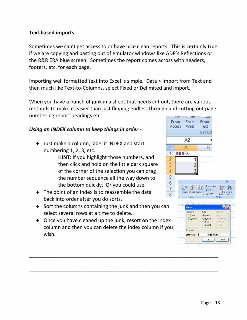
Text based imports  Sometimes we can’t get access to or have nice clean reports.  This is certainly true if we are copying and pasting out of emulator windows like ADP’s Reflections or the R&R ERA blue screen.  Sometimes the report comes across with headers, footers, etc. for each page.  Importing well formatted text into Excel is simple.  Data > Import from Text and then much like Text‐to‐Columns, select Fixed or Delimited and import.    When you have a bunch of junk in a sheet that needs cut out, there are various methods to make it easier than just flipping endless through and cutting out page numbering report headings etc.  Using an INDEX column to keep things in order ‐  

♦ Just make a column, label it INDEX and start numbering 1, 2, 3, etc.   

HINT: If you highlight those numbers, and then click and hold on the little dark square of the corner of the selection you can drag the number sequence all the way down to the bottom quickly.  Or you could use  

♦ The point of an Index is to reassemble the data back into order after you do sorts. 

♦ Sort the columns containing the junk and then you can select several rows at a time to delete. 

♦ Once you have cleaned up the junk, resort on the index column and then you can delete the index column if you wish.  

  ___________________________________________________________________  ___________________________________________________________________  ___________________________________________________________________ 

Page | 14 

In Depth measurements for your department  WHEW!  We took quite a bit of time to get to our examples – but if you don’t understand the work that goes into some of the formulas or capturing the data out of your DMS, the templates or process is meaningless.  

YOUR HEAD IS LIKELY SPINNING RIGHT NOW – THAT’S OK.  We are going to plow through our example templates to explain what is possible and some of the ways to do it.  I am not expecting you to learn the exact process right now – only sit back and take the journey with me.  You have the templates, data, these handouts and access to the recording later to review it again.  ___________________________________________________________________  ___________________________________________________________________  ___________________________________________________________________   First up – Using a template and raw data to populate a chart ‐ Report to graph.xls example.  

• Using a raw text file of a 3611 Report (ADP RAP).  They key isn’t really what report it is as much as where the data ends up. 

• The key for making this example work is that the intermediary sheet called DATA CLEAN.  It pulls the specific data out of the crude cut and paste and then uses it to make the chart. 

o I assume you know how to select a data set to make a chart.  Just highlight the data table and insert a chart.  In this case I prefer it to be on a separate sheet. 

• The “formula” is simply copying from another sheet’s cell o =’DATA PASTE’!E23 o Or get me whatever is in cell E23 on the DATA PASTE sheet 

• You can also use the same syntax in other functions like add, subtract, sum, etc. 

 

Page | 15 

  Gross per RO per Advisor – via a pivot table/chart  The data set is one of the ones we would have cleaned up in the manner we already showed.  Pivot Tables can be tough to get the hang of, but when you do and have a nice data set it takes a lot of the work out of writing formulas, etc.       Menu packages per advisor – via array formulas, named arrays and other way too complex stuff  The best way to do this is prefix/suffix your labor ops with something longer or unique, like 60KMENU.  Then we can pick‐up off the *KMENU text.  In the absences of that we are going to use some brute force.  In the example of our ADP RO DATA, I would use the techniques we have already done to clean up the data to get it down to RO#, ADV# and the Labor Ops.  I would then Find/Replace the potential operations (5K, 30K, etc.) with something like MENUPACKAGE.  Then we could use our =COUNTIF(A2,”MENUPACKAGE”) formula to could up the menu packages per RO.      

Page | 16 

The path less traveled … A much more complex is to make a named range of operations (highly recommend) and then use an array formula.  Array formulas are done by entering the formula and then hitting SHIFT‐CTRL‐ENTER (instead of just enter when you are done with a formula.  If the array is correct, brackets will appear around the formula  

  So this formula is pretty straight forward, let’s read it.  If the sum of cell C2, if it does not have an error, and contains (find) the values in our labor operation group is greater than zero, then the result is true, else false.  Essentially this formula is counting ever occurrence of our labor operation list in a cell and as long as that count is greater than zero it reports “TRUE.”  Once we copy the cells down as is shown in your example, we can select everything, copy, paste special for values only and then work with the table in a Pivot Table. 

 

Page | 17 

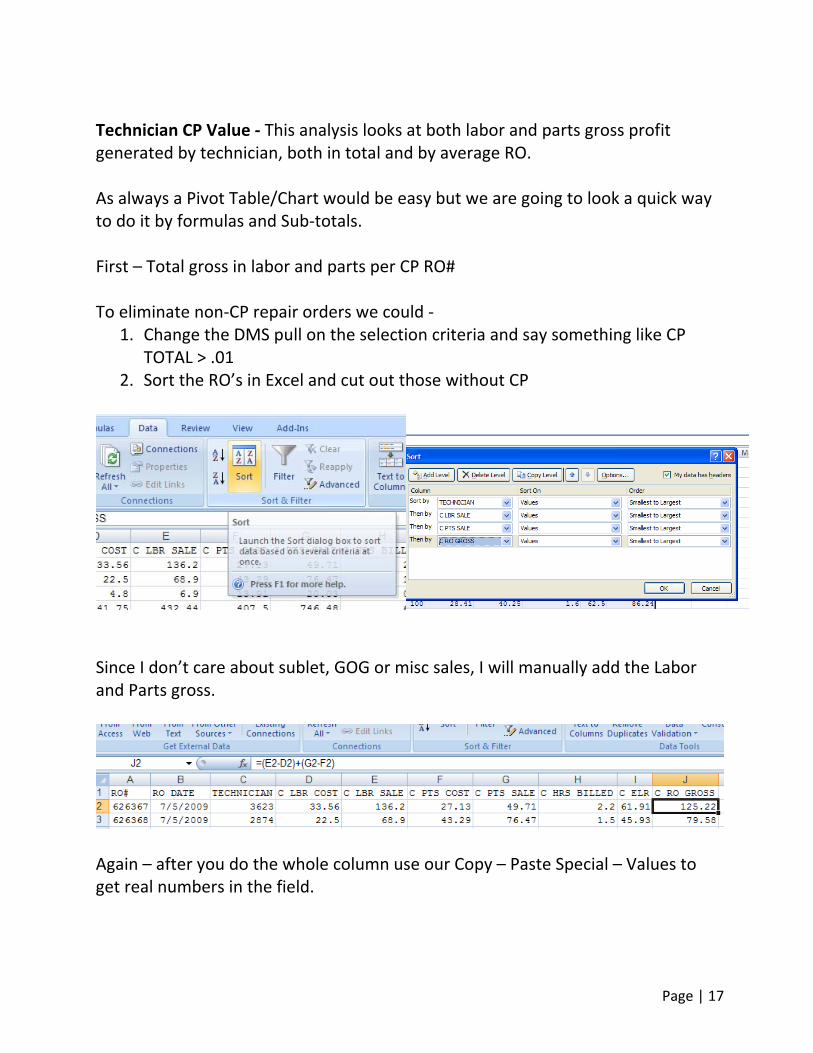
 Technician CP Value ‐ This analysis looks at both labor and parts gross profit generated by technician, both in total and by average RO.  As always a Pivot Table/Chart would be easy but we are going to look a quick way to do it by formulas and Sub‐totals.  First – Total gross in labor and parts per CP RO#  To eliminate non‐CP repair orders we could ‐  

1. Change the DMS pull on the selection criteria and say something like CP TOTAL > .01 

2. Sort the RO’s in Excel and cut out those without CP  

   Since I don’t care about sublet, GOG or misc sales, I will manually add the Labor and Parts gross.  

  Again – after you do the whole column use our Copy – Paste Special – Values to get real numbers in the field.  

Page | 18 

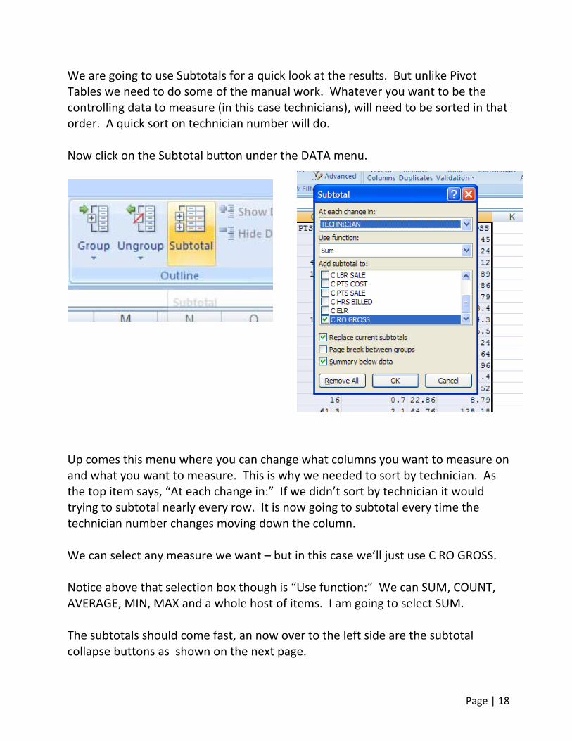
We are going to use Subtotals for a quick look at the results.  But unlike Pivot Tables we need to do some of the manual work.  Whatever you want to be the controlling data to measure (in this case technicians), will need to be sorted in that order.  A quick sort on technician number will do.  Now click on the Subtotal button under the DATA menu.  

        Up comes this menu where you can change what columns you want to measure on and what you want to measure.  This is why we needed to sort by technician.  As the top item says, “At each change in:”  If we didn’t sort by technician it would trying to subtotal nearly every row.  It is now going to subtotal every time the technician number changes moving down the column.  We can select any measure we want – but in this case we’ll just use C RO GROSS.  Notice above that selection box though is “Use function:”  We can SUM, COUNT, AVERAGE, MIN, MAX and a whole host of items.  I am going to select SUM.  The subtotals should come fast, an now over to the left side are the subtotal collapse buttons as  shown on the next page. 

Page | 19 

  See those 1, 2, 3 buttons.  Right now they sheet is showing all the data, the subtotals and the grand total.  By clicking on the buttons we can change the data view to just see the subtotals (by clicking 2 in this example).      

 This is the view showing the subtotal of each technician’s total RO parts and labor gross.    

  This is normally a useful tactic is you are struggling to get the data into something that a Pivot Table will accept or you just want to do a quick view.  By clicking on the plus‐sign + in the left column you can see the individual data sets that make up the total.  Quick Lube Sales – What is the value of your quick lane and its impact on your business results.  Let’s get back to Service Manager Sam from an hour ago.  Something didn’t quite add‐up – advisors were being rewarded for maintaining good gross and ELR, but these were not strong on the factory statement and 20‐group reports.  We dug into those pay plans and found that Sam pulled out certain operations like LOFs.  That is understandable but he also was not looking at the performance of the new 

Page | 20 

Quick Lane he installed last summer.  We did another Pivot Table because it is the easiest.  A couple of things in this template to look at:  Conditional Formatting 

Select the whole set data (such as a whole column of GP% on individual repair orders). 

   

   

 Making a quick chart – While you have selected any cell in the Pivot Table, Insert > and then pick whichever chart you want to see   

 

Page | 21 

  Checking the data – Let’s say we don’t believe those results reported on Quick Lane.  That there might be something strange in there impacting the numbers.  You can hover over whatever cell you want to investigate, (as shown on the image above with the chart where I am hovering over the Quick Lane C LBR GROSS results) double click on it and up will come the actual data set that makes up the calculation in a new sheet.  This can be one of the best features as you drill down to finding opportunity in your shop.    Again, depending on how we format the inquiry from the DMS on the initial pull we could be looking at Labor operations, or vehicle model instead of advisor as shown in this report.    

♦ HINT: Generally, with either ADP or R&R ERA, what you select to sort by in your DMS report will become the dominate data point which all the rest of the data links to. 

  ___________________________________________________________________  ___________________________________________________________________  ___________________________________________________________________ 

Page | 22 

 DON’T FORGET A PLAIN OLD DATA SORT 

  Under the Data menu are the sort features.  For quick work you might be surprised at some of the anomalies in list of 500 repair orders.   In this case, I selected the cell at E1 and just clicked the Smallest to Largest button.  Look at the top result – an RO with a negative gross.  If this did not pop up on our DMS exception report it is something I will want to look at.        Work and Gross mix ‐ The template you have is a manually entry on your initial numbers and then it calculates out from target where your gross profits are being lost.  I use this or a similar template all the time and change the measurements to whatever we suspect is the issue.  Typically besides the measurement which is shown (which is available in this exact format to all GM dealers via your Compass system), you should consider Competitive, Maintenance, Repair divisions. 

Page | 23 

Description of TEMPLATE SAMPLES.XLS  Part Avail – A simple manual form that can have manual entry or be printed for written entry.  An example of table formatting.  Tech time sheet – A mimic of a daily tech time sheet that can be used to measure unapplied time and efficiency.  Efficiency – Table that will calculate technician efficiency when the fields are completed.  Illustrates simple addition and multiplication formulas.  GOG Inv – Shows through a simple formula the month’s supply of GOG.  WTY Inv – Shows through simple formula the month’s supply of warranty claims  Breakeven – through the manual entry of data (orange colored cells) the sheet will calculate what it would take to break‐even.  Various “what‐ifs” can be run by changing your historical data (such as gross profit percentage) to see the impact on your operations.  Net Worksheet – Much like break‐even, but calculates the amount of sales, hours, etc. required to retain 20% gross to the bottom departmental net profit.  Tech Eff Chart – We use this as a quick example in class.  Manually enter information at the top of the sheet and the bottom charts are automatically changed.  Good for bulletin board types of reports.  Labor rate – A labor rate “what if” to show the impact of changing your labor rate.  GP Profit – By entering the data in the yellow cells, this chart will show you how much gross profit was lost or gained by the different RO types.  

Page | 24 

Serv Adv Pay – By entering in the data in the blue cells, this work sheet will help formulate a pay plan that is structured at certain goals and target incomes.  Attendance Sheet – A simple table for showing percentage of attendance.  The purpose is to also show an example of the COUNTA function in columns AG and AH.  S. Adv Box Performance – This is a complex sheet that is prone to “breaking”.  Essentially through the data set (which can be imported) at the bottom of the chart, it gives the performance range of the advisors which a much more clear picture than simple averages.  

Page | 25 

 

Shop measurements to consider Demographics 

• Model and year mix % • Vehicle mileage mix % 

 Overall Shop Performance Indexes 

• Effective Labor rates by labor type (competitive, maintenance, repair) • % of work mix (competitive, maintenance, repair) by labor hours paid • One‐Item RO (modified to remove N/C lines and internal and warranty 

lines) • Menu penetration; including Good, Better, Best recommendations • Number of Customer Pay ROs • Unapplied labor average per RO 

 COGS and/or Gross Profit percentage for shop 

• Total labor sales/Total labor gross • Sales per RO • Gross per RO • FRH per RO • CP total gross as a % 

 Individual Advisor statistics 

• # of ROs written and pay type % C/W/I • Average days ROs are open • Average ROs per day • % of total shop sales • % of total shop gross • Average  FRH/day • Average FRH/RO • Effective labor rate – also broken by competitive/maintenance/repair • Parts to labor ratio • Lines per repair order  • Menu package opportunities and % closed 

Product Page: Links direct from ad, email or from entry page