30 Microsoft®Excel® Tips and Tricks - RKL eSolutions, LLC · PDF file30 Microsoft®Excel® Tips and Tricks Microsoft Excel 2007, 2010 & 2013 Functions & Formulas PivotTables & PivotCharts

30 Microsoft®Excel® Tips and Tricks

Microsoft Excel 2007, 2010 & 2013

Functions & FormulasPivotTables & PivotCharts

Data FormattingKeyboard Shortcuts

2

Excel Tips & Tricks

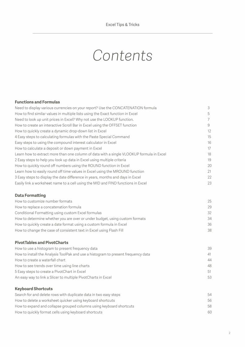
Contents

Functions and FormulasNeed to display various currencies on your report? Use the CONCATENATION formula 3How to find similar values in multiple lists using the Exact function in Excel 5Need to look up unit prices in Excel? Why not use the LOOKUP function. 7How to create an interactive Scroll Bar in Excel using the OFFSET function 9How to quickly create a dynamic drop-down list in Excel 124 Easy steps to calculating formulas with the Paste Special Command 15Easy steps to using the compound interest calculator in Excel 16How to calculate a deposit or down payment in Excel 17Learn how to extract more than one column of data with a single VLOOKUP formula in Excel 182 Easy steps to help you look up data in Excel using multiple criteria 19How to quickly round off numbers using the ROUND function in Excel 20Learn how to easily round off time values in Excel using the MROUND function 213 Easy steps to display the date difference in years, months and days in Excel 22Easily link a worksheet name to a cell using the MID and FIND functions in Excel 23

Data FormattingHow to customize number formats 25How to replace a concatenation formula 29Conditional Formatting using custom Excel formulas 32How to determine whether you are over or under budget, using custom formats 34How to quickly create a date format using a custom formula in Excel 36How to change the case of consistent text in Excel using Flash Fill 38

PivotTables and PivotChartsHow to use a histogram to present frequency data 39How to install the Analysis ToolPak and use a histogram to present frequency data 41 How to create a waterfall chart 44How to see trends over time using line charts 485 Easy steps to create a PivotChart in Excel 51An easy way to link a Slicer to multiple PivotCharts in Excel 53

Keyboard ShortcutsSearch for and delete rows with duplicate data in two easy steps 54How to delete a worksheet quicker using keyboard shortcuts 56How to expand and collapse grouped columns using keyboard shortcuts 58How to quickly format cells using keyboard shortcuts 60

3

30 Excel Tips & TricksFunctions & Formulas

Need to display various currencies on your report? Use the CONCATENATION formulaFormatting cells allows you to change the way data is presented, without affecting the contents of the cell. Say for example you need to create a sales report to display the value of sales in various countries in each country’s currency, you can apply the CONCATENATION formula, instead of having to manually change each cell to display the relevant currency for each country

Download the workbook to practice.

Applies to: Microsoft Excel 2007, 2010 and 2013.

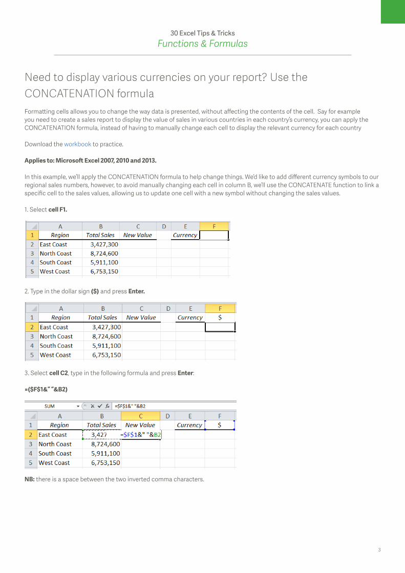
In this example, we’ll apply the CONCATENATION formula to help change things. We’d like to add different currency symbols to our regional sales numbers, however, to avoid manually changing each cell in column B, we’ll use the CONCATENATE function to link a specific cell to the sales values, allowing us to update one cell with a new symbol without changing the sales values.

1. Select cell F1.

2. Type in the dollar sign ($) and press Enter.

3. Select cell C2, type in the following formula and press Enter:

=($F$1&” “&B2)

NB: there is a space between the two inverted comma characters.

http://www.sagedl.com/sage-email/PDFs/TEXT%20Functions%20-%20Concatenation.xlsx

4


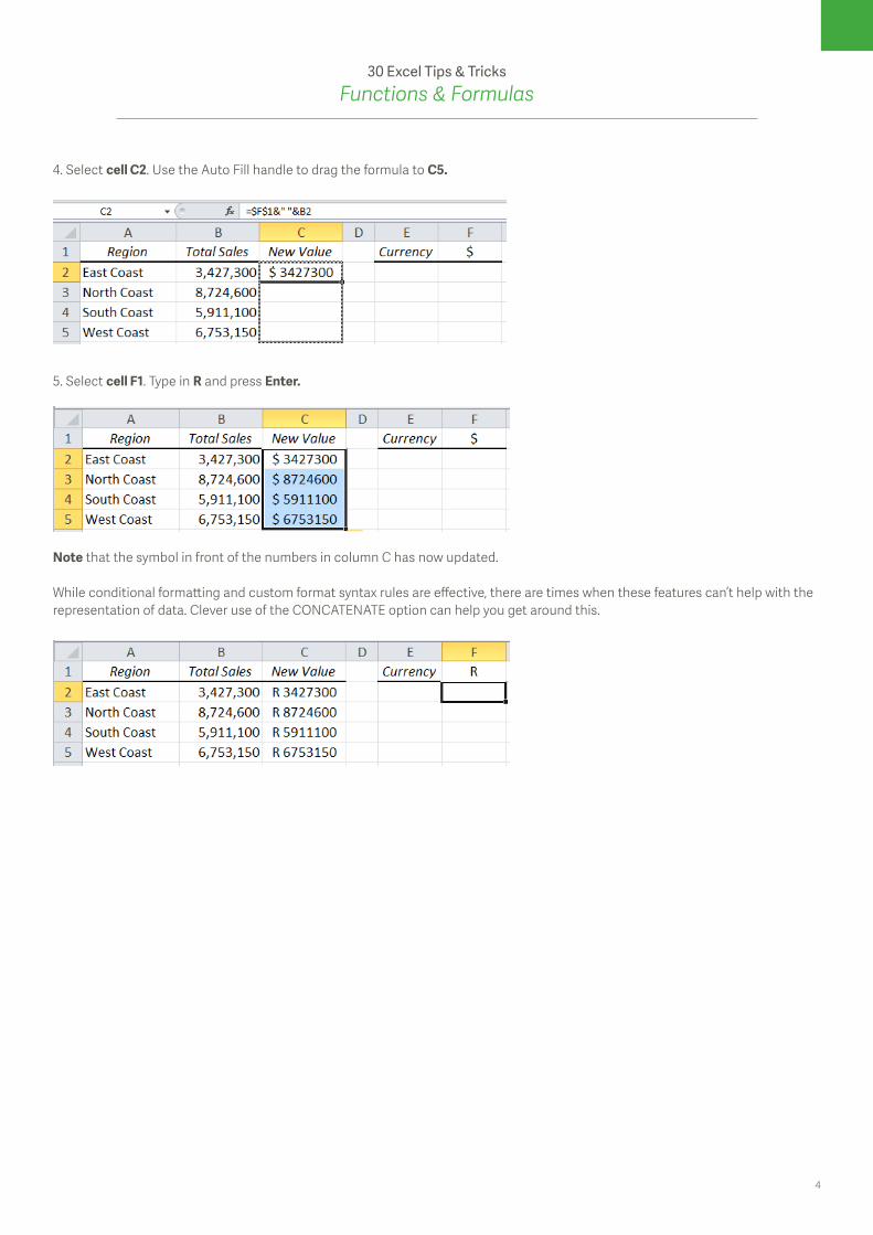
4. Select cell C2. Use the Auto Fill handle to drag the formula to C5.

5. Select cell F1. Type in R and press Enter.

Note that the symbol in front of the numbers in column C has now updated.

While conditional formatting and custom format syntax rules are effective, there are times when these features can’t help with the representation of data. Clever use of the CONCATENATE option can help you get around this.

5


How to find similar values in multiple lists using the Exact function in ExcelMicrosoft® Excel® provides an easy way to find similar values between multiple lists using the Exact function in Excel. By applying this function you will be able to find out the exact match between two strings of data. When you are working in Excel, text differences within a cell can often be troublesome, that’s why it is important to identify and remove varying information.

In our example, we explain how you can use the Exact function to compare two product lists. We’ll work through the spreadsheet and compare client details as an accounts clerk to ensure that the information is the same.

Apply the Exact function to check whether two text strings are exactly the same. It will return the following results; TRUE if they match and FALSE if otherwise. It is important to note that the Exact function is also case sensitive.

Download the workbook to practice

Applies to: Microsoft Excel 2010 and 2013

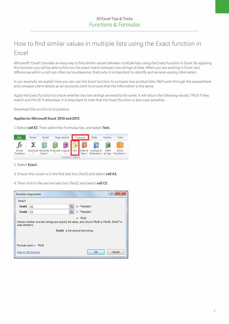
1. Select cell E2. Then select the Formulas tab, and select Text.

2. Select Exact.

3. Ensure the cursor is in the first text box (Text1) and select cell A2.

4. Then click in the second text box (Text2) and select cell C2.

http://www.sagedl.com/sage-email/PDFs/01.07.2015_How%20to%20check%20for%20discrepancies%20between%20text%20strings.xlsx

6


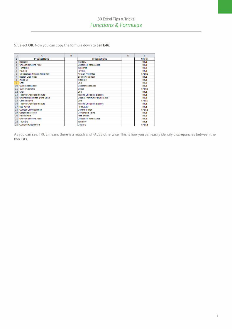
5. Select OK. Now you can copy the formula down to cell E46.

As you can see, TRUE means there is a match and FALSE otherwise. This is how you can easily identify discrepancies between the two lists.

7


Need to look up unit prices in Excel? Why not use the LOOKUP function.In this tip we’ll show you how to look up unit prices in your workbook using the LOOKUP function in Excel. The LOOKUP function is an alternative method to the more commonly used VLOOKUP function in Microsoft® Excel®.

Manually entering data in your workbook can lead to inaccuracies with your information, you can apply the LOOKUP function to avoid that.

The LOOKUP function can be used to look up data in single row or column range, it searches for the value in the first row or column and returns a value from the same position in the second row or column range selected. The data being searched will be sorted in ascending order.

In our example, we use the LOOKUP function, using the vector form method, to return the unit price for items.


Applies to: Microsoft® Excel® 2010 and 2013

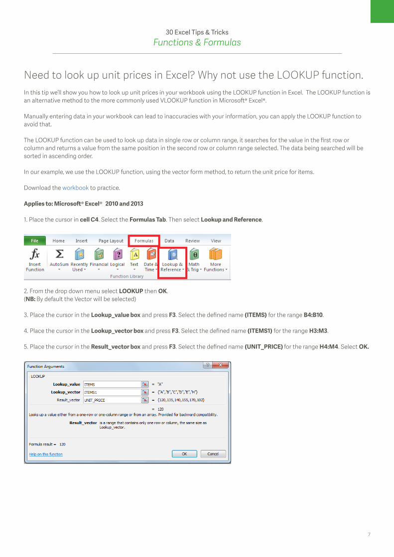
1. Place the cursor in cell C4. Select the Formulas Tab. Then select Lookup and Reference.

2. From the drop down menu select LOOKUP then OK.(NB: By default the Vector will be selected)

3. Place the cursor in the Lookup_value box and press F3. Select the defined name (ITEMS) for the range B4:B10.

4. Place the cursor in the Lookup_vector box and press F3. Select the defined name (ITEMS1) for the range H3:M3.

5. Place the cursor in the Result_vector box and press F3. Select the defined name (UNIT_PRICE) for the range H4:M4. Select OK.

http://www.sagedl.com/sage-email/PDFs/08.07.2015_How%20to%20lookup%20data%20with%20the%20lookup%20function.xlsx

8


6. Copy the formula down to cell C10.

The unit prices have been looked up without having to manually enter them. This will ensure that your data is accurate, whilst saving you time and making your process more efficient.

9


How to create an interactive Scroll Bar in Excel using the OFFSET functionEver wondered how to create an interactive Scroll Bar in Microsoft® Excel®? Instead of manually typing in a particular month or value, you can use the Scroll Bar control to select the months or values from a list, thus saving your time. In this week’s tip we’ll show you how by using the Offset function along with the Scroll Bar.

The OFFSET function returns a cell or range of cells that is a specified number of rows and or columns within your spreadsheet. The range of cells is given a starting point with specified height (number of rows) and width (number of columns). You can use the OFFSET function to select a dynamic cell reference.

In this example we’ll demonstrate how Months can be interactively selected with the Scroll Bar control and the OFFSET function.



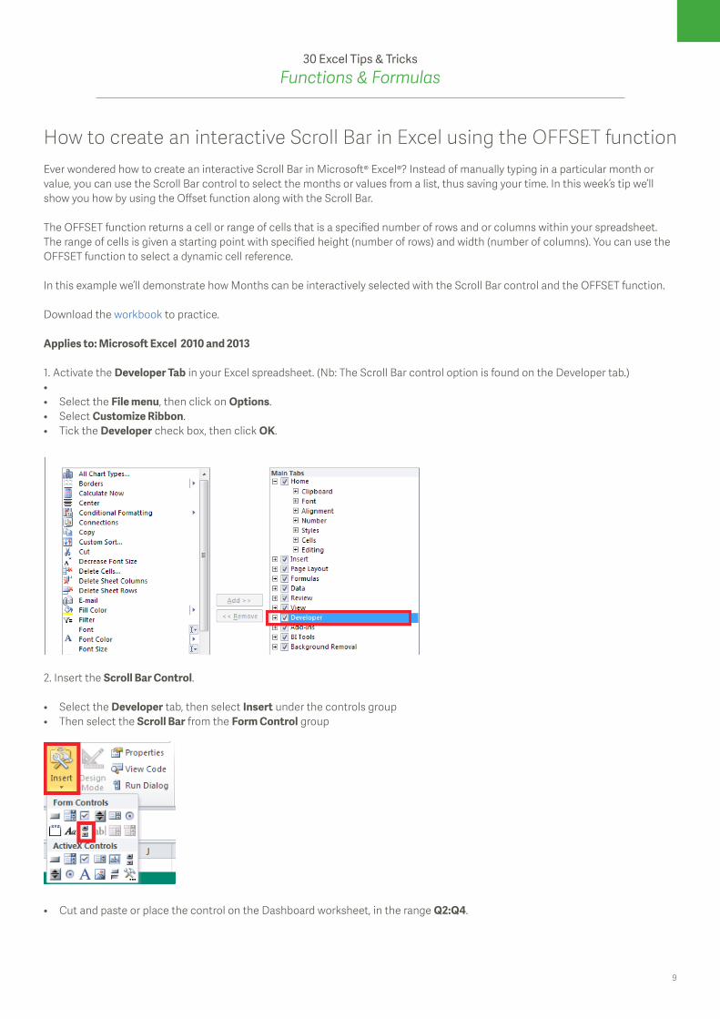
1. Activate the Developer Tab in your Excel spreadsheet. (Nb: The Scroll Bar control option is found on the Developer tab.)• • Select the File menu, then click on Options. • Select Customize Ribbon.• Tick the Developer check box, then click OK.

2. Insert the Scroll Bar Control.

• Select the Developer tab, then select Insert under the controls group• Then select the Scroll Bar from the Form Control group

• Cut and paste or place the control on the Dashboard worksheet, in the range Q2:Q4.

http://www.sagedl.com/sage-email/PDFs/1.%2016.07.2015_Creating%20an%20interactive%20Scroll%20Bar%20Control%20by%20using%20the%20Offset%20formula.xlsx

10


3. Format the Scroll Bar Control (NB: To make the Scroll Bar control interactive using the OFFSET formula, you first need to change some of the Scroll Bar Control settings.)

• Right click on the Scroll Bar Control, then select the Format Control menu item.• Set the maximum value to 11 (number of months, excluding the starting point which makes it 12).• Click the red arrow (edit reference icon) in the Cell link.• On the Lists worksheet, select cell B14 (the output of the Scroll Bar, a number representing the selected month).• Then select the red arrow (edit reference icon) to return to the Format Control window, then select the OK button.

4. Using the OFFSET function to return the month name.

• Select the Dashboard worksheet, then select cell N3.• Select the Formulas tab, then select Lookup & Reference.• Select OFFSET.

Complete the fields as follows:

Reference: the specified starting point.Rows: Number of rows you want to move from the starting point.Cols: Number of columns you want to move from the starting point.Height: This is the size in rows of the range you want to be returned.Width: This is the size in columns of the range you want to be returned.

11


• Select the red arrow (edit reference icon) in the Reference.• Select cell B1 on the lists worksheet, then select the red arrow (edit reference icon) to return.• Select the red arrow (edit reference icon) in the Rows.• Select cell B14 on the Lists, then select the red arrow (edit reference icon) to return.• Place your cursor in the Cols box, enter 0 and select OK.

The months can now be interactively selected by using the Scroll Bar Control.

12


How to quickly create a dynamic drop-down list in ExcelA dynamic drop down list in Microsoft® Excel® is a convenient way of selecting data without making changes to the source. Let’s say you have a list where you are likely to add or remove values, a dynamic drop down would be the best option to select data. With a dynamic drop-down list, when you delete or add months the list changes to accommodate that action, whereas a normal list does not.

We have written tips on how to create a static and dynamic drop down list using and the Table option. However, in this tip we show you how to create a dynamic drop down list by using Data Validation, OFFSET and COUNTA functions.

We learnt in our previous tip that the OFFSET function is used for creating dynamic data ranges. The COUNTA function counts the number of cells that are not empty in a range. Data Validation is used for restricting what type of data should or can be entered into a range.



1. We start by creating a defined name.

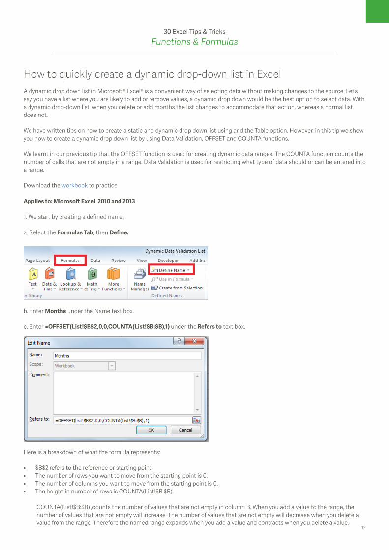
a. Select the Formulas Tab, then Define.

b. Enter Months under the Name text box.

c. Enter =OFFSET(List!$B$2,0,0,COUNTA(List!$B:$B),1) under the Refers to text box.

Here is a breakdown of what the formula represents:

• $B$2 refers to the reference or starting point.• The number of rows you want to move from the starting point is 0.• The number of columns you want to move from the starting point is 0.• The height in number of rows is COUNTA(List!$B:$B).

COUNTA(List!$B:$B) ,counts the number of values that are not empty in column B. When you add a value to the range, the number of values that are not empty will increase. The number of values that are not empty will decrease when you delete a value from the range. Therefore the named range expands when you add a value and contracts when you delete a value.

http://www.sagedl.com/sage-email/PDFs/22.07.2015_How%20to%20create%20a%20dynamic%20drop%20down%20list.xlsx

13


• The width in number of columns is 1.

d. Select OK.

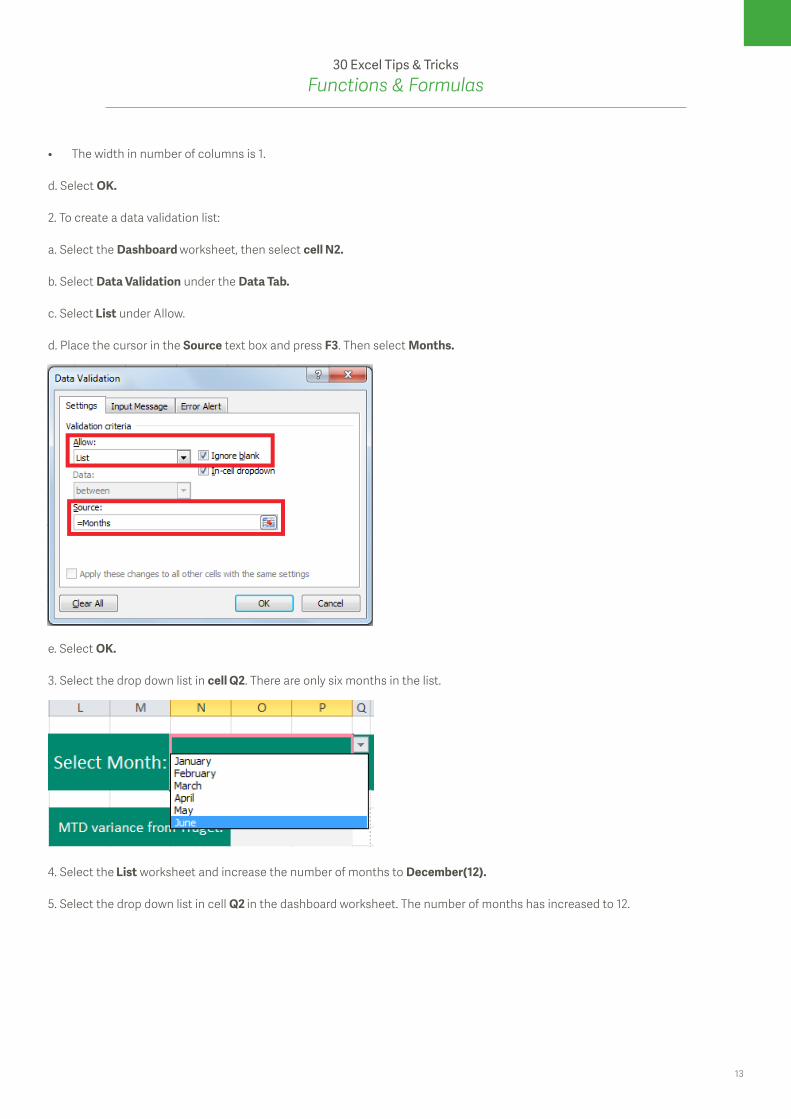
2. To create a data validation list:

a. Select the Dashboard worksheet, then select cell N2.

b. Select Data Validation under the Data Tab.

c. Select List under Allow.

d. Place the cursor in the Source text box and press F3. Then select Months.

e. Select OK.

3. Select the drop down list in cell Q2. There are only six months in the list.

4. Select the List worksheet and increase the number of months to December(12).

5. Select the drop down list in cell Q2 in the dashboard worksheet. The number of months has increased to 12.

14


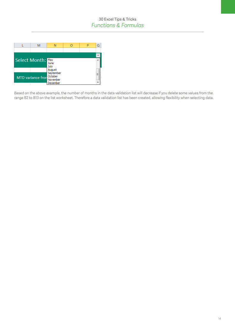
Based on the above example, the number of months in the data validation list will decrease if you delete some values from the range B2 to B13 on the list worksheet. Therefore a data validation list has been created, allowing flexibility when selecting data.

15


4 Easy steps to calculating formulas with the Paste Special CommandHave you ever wondered how to use the formulas operations under the Paste special command? You can divide, add, multiply and subtract values when you copy and paste.

Let’s say, you want to quickly convert values from millions to thousands when you copy and paste, you can use the paste special divide formula. This command will save you time creating normal formulas to carry out this instruction. Furthermore, the values will be easy to analyse when converted to a lower value.



1. Start by highlighting the divider range, D3 to D20.

2. Right click and copy. Then highlight the values range, C3 to C20.

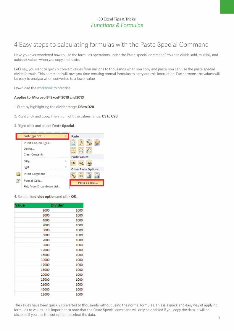
3. Right click and select Paste Special.

4. Select the divide option and click OK.

The values have been quickly converted to thousands without using the normal formulas. This is a quick and easy way of applying formulas to values. It is important to note that the Paste Special command will only be enabled if you copy the data. It will be disabled if you use the cut option to select the data.

http://www.sagedl.com/sage-email/PDFs/26.08.2015_Calculating%20Formulas%20with%20the%20Pastel%20Special%20Command.xlsx

16


Easy steps to using the compound interest calculator in ExcelMy daughter just completed a project of creating a piggy bank at school. This reminded me of the importance of saving. The return on investment is often determined by interest rates and this is why investors or anyone who wants to save chooses the right moment to make an investment.

In this tip we explain how to calculate compound interest using Microsoft® Excel®.

Since there is no standard function to calculate compound interest in Excel, we’ll show you how to create a custom compound interest function.



Compound interest is interest paid on both the original amount of money and on the interest it has already earned. Follow the steps below as we explain how:

1. Press ALT & F11 to start the Visual Basic editor.2. Select Module from the Insert menu.3. Copy and Paste the following code:

Function Compound_Rate(PV As Double, R As Double, N As Double) As DoubleCompound_Rate = PV*(1+R)^NEnd Function

Note:• A function returns a value.• Double is a data type that has a fractional component.• PV is the Present value of the Investment.• R is the interest rate.• N is the number of investment periods.

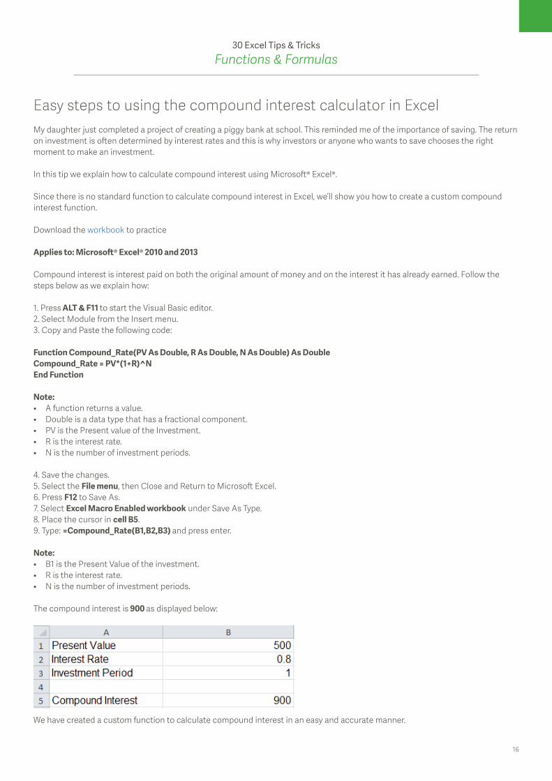
4. Save the changes.5. Select the File menu, then Close and Return to Microsoft Excel.6. Press F12 to Save As.7. Select Excel Macro Enabled workbook under Save As Type.8. Place the cursor in cell B5.9. Type: =Compound_Rate(B1,B2,B3) and press enter.

Note:• B1 is the Present Value of the investment.• R is the interest rate.• N is the number of investment periods.

The compound interest is 900 as displayed below:

We have created a custom function to calculate compound interest in an easy and accurate manner.

http://www.sagedl.com/sage-email/PDFs/03.09.2015_How%20to%20calculate%20compound%20interest.xlsm

17


How to calculate a deposit or down payment in ExcelPurchasing a car or a house is usually a pleasant experience for the buyer. However, most financial institutions require a deposit or down payment to be made towards the total purchase price.

In this week’s tip, we share how to calculate the deposit or down payment for a car. For instance, the cost of the car could be $15,000 to be repaid over four years at 3% per period. Furthermore, you may want to keep the monthly payment at $400 per month, but need to calculate the deposit. This is how it can be done:



1. We are going to use the following formula:

=Purchase Price-PV(Rate,Nper,-Pmt)

• PV: calculates the loan amount.• The loan amount will be subtracted from the purchase price to get the deposit amount.• Rate: is the interest rate per period. It will be divided by 4 if per quarter or 12 if it’s per annum.• Nper: is the total number of payment periods in an investment, which will be 48(4*12).• Pmt: is the payment made each period.

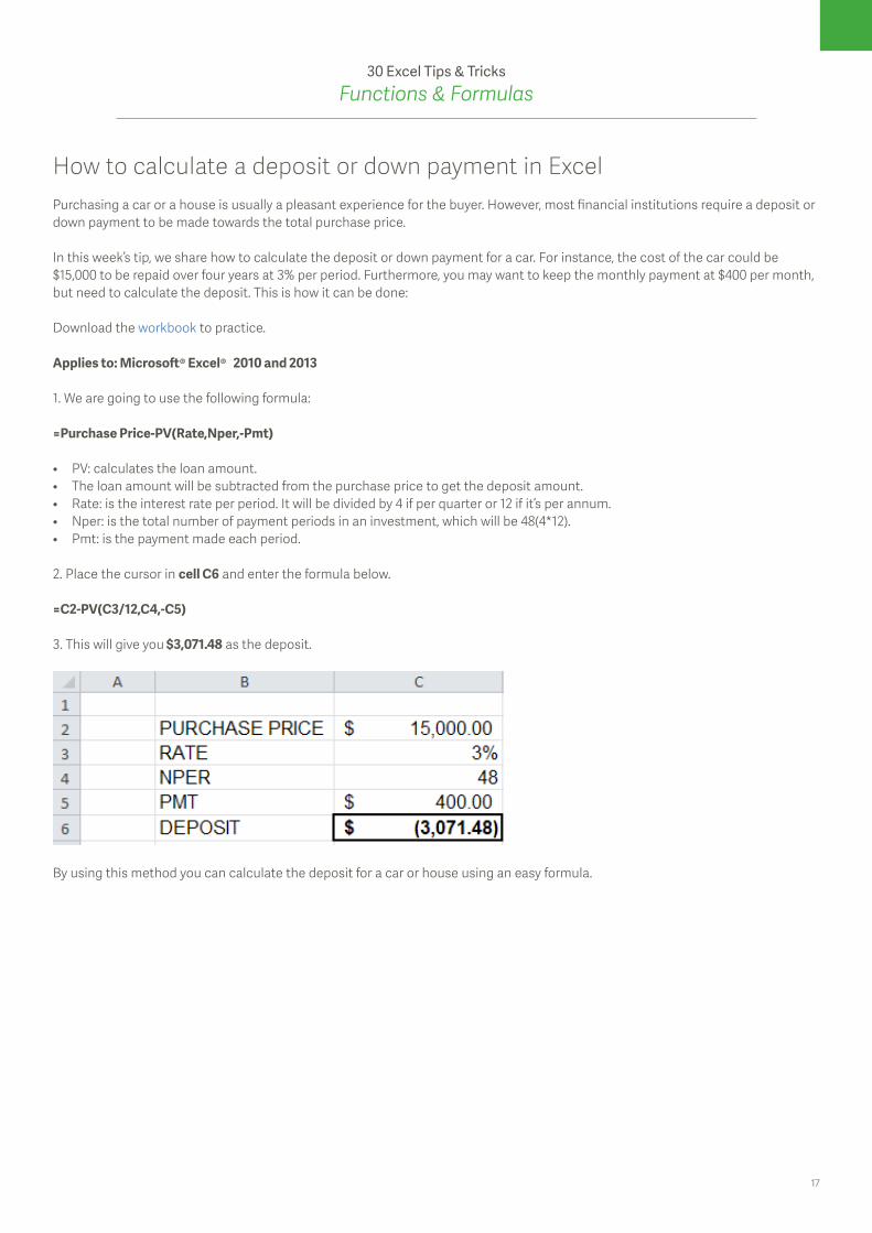
2. Place the cursor in cell C6 and enter the formula below.

=C2-PV(C3/12,C4,-C5)

3. This will give you $3,071.48 as the deposit.

By using this method you can calculate the deposit for a car or house using an easy formula.

http://www.sagedl.com/sage-email/PDFs/10.09.2015_How%20to%20calculate%20the%20deposit%20or%20down%20payment.xlsx

18


Learn how to extract more than one column of data with a single VLOOKUP formula in ExcelIt’s over 10 years since I started training Microsoft® Excel® to corporate clients. During training sessions, delegates usually ask questions on how they can use Excel to help them become more effective in their work. Last week, a financial manager asked me how she could easily look up more than one field of data from a table with a single VLOOKUP formula.

She wanted to extract the product name, customer name and selling price using one VLOOKUP formula. Her concern was the time it took to extract one field. I therefore, decided to write this tip with a view of helping someone save time and increase productivity.



1. We are going to extract the product name, customer name and selling price with one VLOOKUP formula. This is the formula we are going to use:

=VLOOKUP(Lookup_value,Table Array,{3,4,6},Range_Lookup)

• Lookup_Value is the common field between the data range and the extraction table.• Table Array is the source data range.• The curly brackets represent the position of the fields to be extracted in the source data range. This is not linked to the column

letter, but it is the position of the field to be extracted within the table.• Range_Lookup is either an exact or approximate match

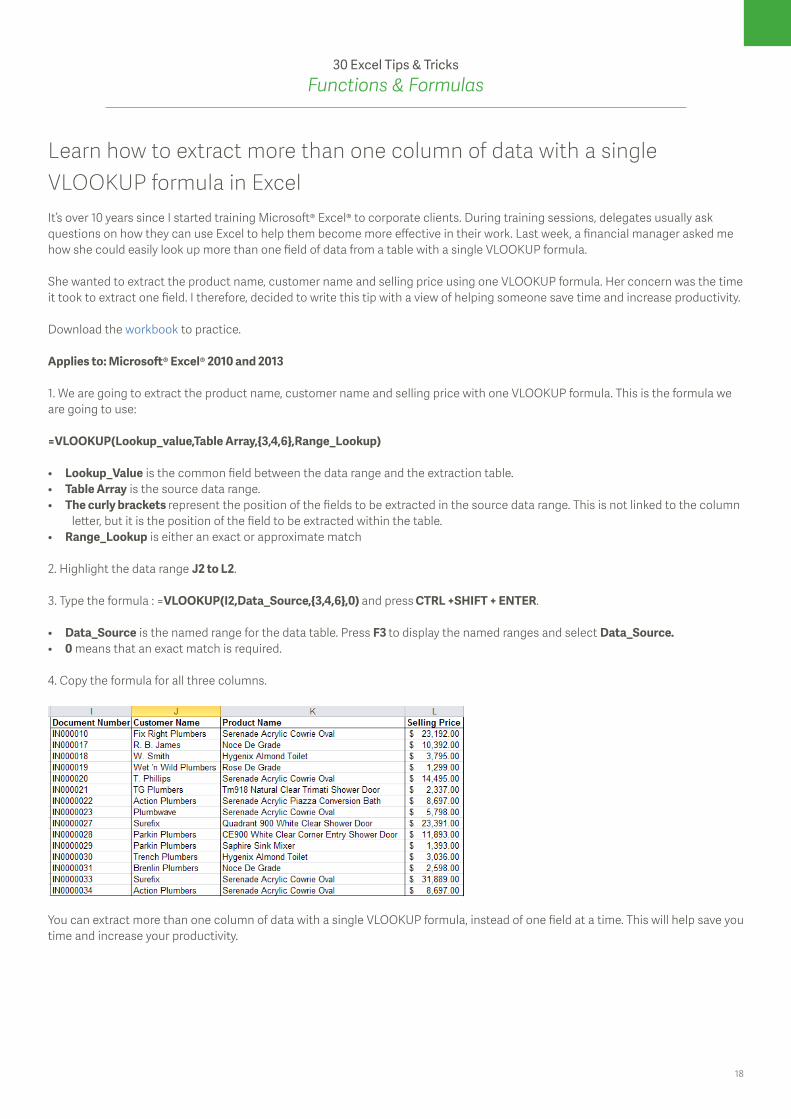
2. Highlight the data range J2 to L2.

3. Type the formula : =VLOOKUP(I2,Data_Source,{3,4,6},0) and press CTRL +SHIFT + ENTER.

• Data_Source is the named range for the data table. Press F3 to display the named ranges and select Data_Source.• 0 means that an exact match is required.

4. Copy the formula for all three columns.

You can extract more than one column of data with a single VLOOKUP formula, instead of one field at a time. This will help save you time and increase your productivity.

http://www.sagedl.com/sage-email/PDFs/17.09.205_How%20to%20extract%20more%20than%20one%20column%20of%20data%20with%20a%20single%20Vlookup%20formula.xlsx

19


2 Easy steps to help you look up data in Excel using multiple criteriaWe showed you how to extract more than one column of data with a single Vlookup formula. However, if you want to look up data with multiple criteria then you can use the INDEX and MATCH functions.

You can look up data that meets multiple criteria and overcome the limitations of the Vlookup, thus saving you time and making your process more efficient.

Follow the example below, as I explain how to use the invoice number and order number to extract the customer’s name.


Applies to: Microsoft® Excel® 2010 and 2013.

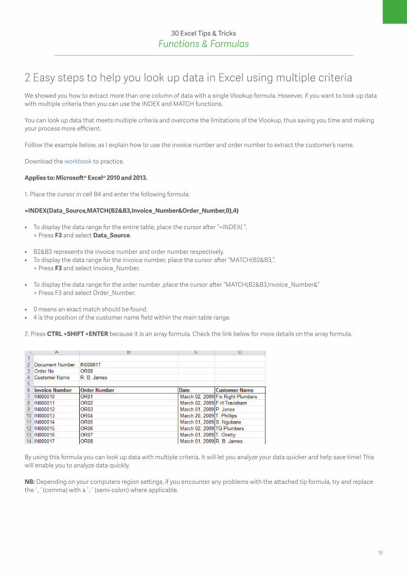
1. Place the cursor in cell B4 and enter the following formula:

=INDEX(Data_Source,MATCH(B2&B3,Invoice_Number&Order_Number,0),4)

• To display the data range for the entire table, place the cursor after “=INDEX( “. > Press F3 and select Data_Source.

• B2&B3 represents the invoice number and order number respectively.• To display the data range for the invoice number, place the cursor after “MATCH(B2&B3,”. > Press F3 and select Invoice_Number.

• To display the data range for the order number ,place the cursor after “MATCH(B2&B3,Invoice_Number&” > Press F3 and select Order_Number.

• 0 means an exact match should be found.• 4 is the position of the customer name field within the main table range.

2. Press CTRL +SHIFT +ENTER because it is an array formula. Check the link below for more details on the array formula.

By using this formula you can look up data with multiple criteria. It will let you analyze your data quicker and help save time! This will enable you to analyze data quickly.

NB: Depending on your computers region settings, if you encounter any problems with the attached tip formula, try and replace the ‘ , ‘ (comma) with a ‘ ; ‘ (semi-colon) where applicable.

http://www.sagedl.com/sage-email/PDFs/28.09.2015_Index%20&%20Match%20Functions.xlsx

20


How to quickly round off numbers using the ROUND function in ExcelAnyone who works with figures in Microsoft® Excel® knows the importance of quickly rounding off numbers. Luckily Excel has an easy function that allows you to round off numbers without any hassle.

Instead of clicking the increase or decrease decimal options on the ribbon, you can use the ROUND function to round off numbers to a specified number of decimal digits. In the next tip we will explain how to round off seconds to minutes using the MROUND function.



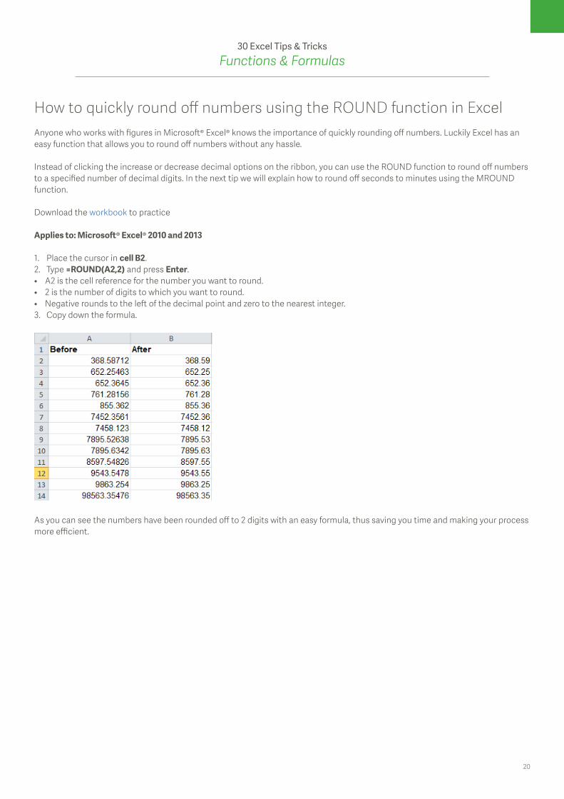
1. Place the cursor in cell B2.2. Type =ROUND(A2,2) and press Enter.• A2 is the cell reference for the number you want to round.• 2 is the number of digits to which you want to round. • Negative rounds to the left of the decimal point and zero to the nearest integer.3. Copy down the formula.

As you can see the numbers have been rounded off to 2 digits with an easy formula, thus saving you time and making your process more efficient.

http://www.sagedl.com/sage-email/PDFs/01.10.2015_How%20to%20quickly%20round%20off%20numbers.xlsx

21


Learn how to easily round off time values in Excel using the MROUND functionWorking with time values comes with its own challenges. One of the issues is how to round off time values from seconds to minutes or minutes to hours.

You can use the MROUND function to round off time values. The MROUND function returns a number rounded to the nearest instance of a specified multiple.

It’s easier to manipulate time values if they are rounded off. So, if you work with time values you will find this tip useful, especially HR personnel, IT security professionals, stock controllers etc.



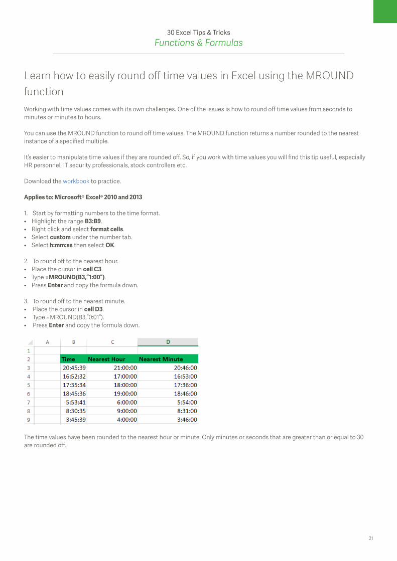
1. Start by formatting numbers to the time format.• Highlight the range B3:B9.• Right click and select format cells.• Select custom under the number tab.• Select h:mm:ss then select OK.

2. To round off to the nearest hour.• Place the cursor in cell C3.• Type =MROUND(B3,”1:00”).• Press Enter and copy the formula down.

3. To round off to the nearest minute.• Place the cursor in cell D3.• Type =MROUND(B3,”0:01”).• Press Enter and copy the formula down.

The time values have been rounded to the nearest hour or minute. Only minutes or seconds that are greater than or equal to 30 are rounded off.

http://www.sagedl.com/sage-email/PDFs/08.010.2015_How%20to%20quickly%20round%20off%20time.xlsx

22


3 Easy steps to display the date difference in years, months and days in ExcelRecently an HR consultant asked how she could show the time served by employees in years, months and days. She currently only displays the time served in years and wanted to be more specific. An inventory controller also asked me a similar question in relation to stock movement.

Therefore we will practice using the DATEDIF and concatenate functions. The DATEDIF function returns the difference between two dates and the concatenate function joins the various formulas into one function.



1. Select the Practice worksheet.2. Place the cursor in cell C4.3. Enter the formula below.

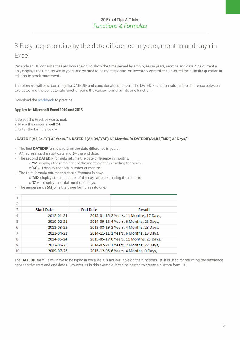
=DATEDIF(A4,B4,”Y”) &” Years, “ & DATEDIF(A4,B4,”YM”) & “ Months, “& DATEDIF(A4,B4,”MD”) &” Days,”

• The first DATEDIF formula returns the date difference in years.• A4 represents the start date and B4 the end date.• The second DATEDIF formula returns the date difference in months. o YM’ displays the remainder of the months after extracting the years. o ‘M’ will display the total number of months.• The third formula returns the date difference in days. o ‘MD’ displays the remainder of the days after extracting the months. o ‘D’ will display the total number of days.• The ampersands (&) joins the three formulas into one.

The DATEDIF formula will have to be typed in because it is not available on the functions list. It is used for returning the difference between the start and end dates. However, as in this example, it can be nested to create a custom formula .

http://www.sagedl.com/sage-email/PDFs/5.11.2015_How%20to%20display%20the%20date%20difference%20in%20years%20months%20and%20days.xlsx

23


Easily link a worksheet name to a cell using the MID and FIND functions in ExcelReports are often prepared and presented on a regular basis. Some businesses often use Microsoft® Excel® to present their reports. Report headings can contain worksheet names and that is why it is important to link worksheet names to a cell. This can be achieved by using the MID and FIND functions in Excel. This will save you the time of re-typing the worksheet names in the report headings.

Using the steps below you can have your worksheet names for each month in a workbook and display the worksheet names in the report heading automatically.



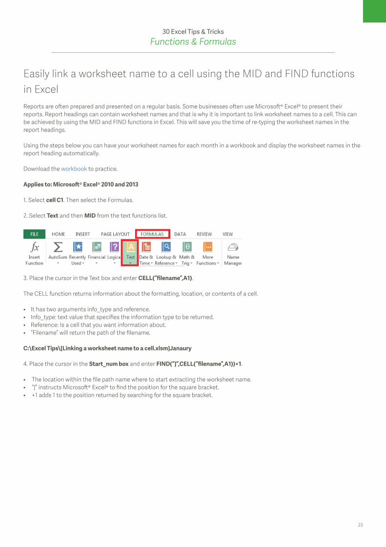
1. Select cell C1. Then select the Formulas.

2. Select Text and then MID from the text functions list.

3. Place the cursor in the Text box and enter CELL(“filename”,A1).

The CELL function returns information about the formatting, location, or contents of a cell.

• It has two arguments info_type and reference.• Info_type: text value that specifies the information type to be returned.• Reference: Is a cell that you want information about.• “Filename” will return the path of the filename.

C:\Excel Tips\[Linking a worksheet name to a cell.xlsm]Janaury

4. Place the cursor in the Start_num box and enter FIND(“]”,CELL(“filename”,A1))+1.

• The location within the file path name where to start extracting the worksheet name.• “]” instructs Microsoft® Excel® to find the position for the square bracket.• +1 adds 1 to the position returned by searching for the square bracket.

http://www.sagedl.com/sage-email/PDFs/12.11.2015_Linking%20a%20worksheet%20name%20to%20a%20cell.xlsm

24


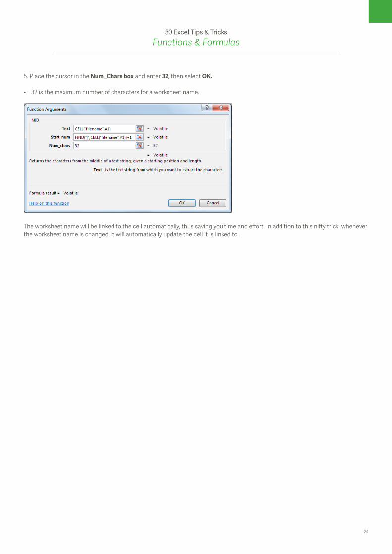
5. Place the cursor in the Num_Chars box and enter 32, then select OK.

• 32 is the maximum number of characters for a worksheet name.

The worksheet name will be linked to the cell automatically, thus saving you time and effort. In addition to this nifty trick, whenever the worksheet name is changed, it will automatically update the cell it is linked to.

25

30 Excel Tips & TricksData Formatting

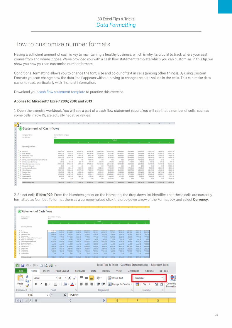
How to customize number formatsHaving a sufficient amount of cash is key to maintaining a healthy business, which is why it’s crucial to track where your cash comes from and where it goes. We’ve provided you with a cash flow statement template which you can customise. In this tip, we show you how you can customise number formats.

Conditional formatting allows you to change the font, size and colour of text in cells (among other things). By using Custom Formats you can change how the data itself appears without having to change the data values in the cells. This can make data easier to read, particularly with financial information.

Download your cash flow statement template to practice this exercise.

Applies to: Microsoft® Excel® 2007, 2010 and 2013

1. Open the exercise workbook. You will see a part of a cash flow statement report. You will see that a number of cells, such as some cells in row 19, are actually negative values.

2. Select cells E14 to P29. From the Numbers group, on the Home tab, the drop down list identifies that these cells are currently formatted as Number. To format them as a currency values click the drop down arrow of the Format box and select Currency.

http://www.sagedl.com/sage-email/PDFs/Cashflow%20Statement%20-%20Number%20Formats.xlsx

26


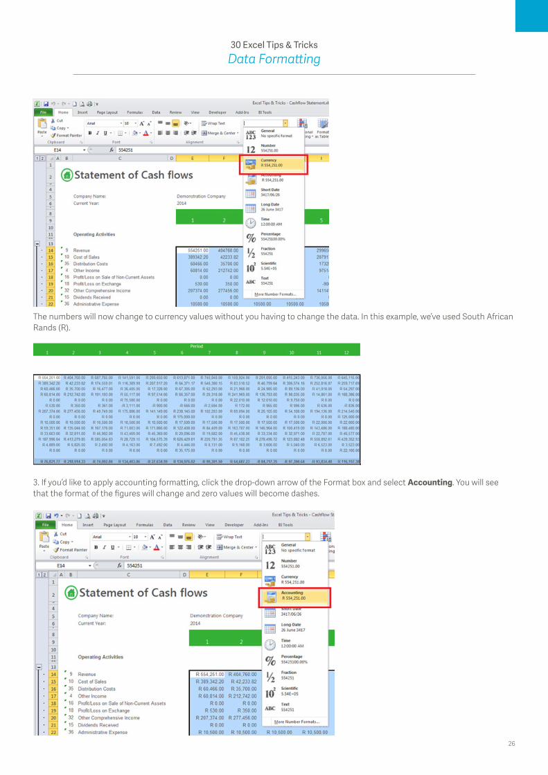
The numbers will now change to currency values without you having to change the data. In this example, we’ve used South African Rands (R).

3. If you’d like to apply accounting formatting, click the drop-down arrow of the Format box and select Accounting. You will see that the format of the figures will change and zero values will become dashes.

27


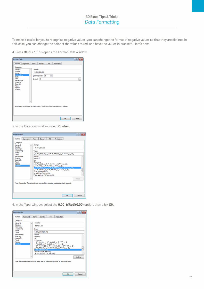
To make it easier for you to recognise negative values, you can change the format of negative values so that they are distinct. In this case, you can change the color of the values to red, and have the values in brackets. Here’s how:

4. Press CTRL + 1. This opens the Format Cells window.

5. In the Category window, select Custom.

6. In the Type: window, select the 0.00_);[Red](0.00) option, then click OK.

28


You will now see the negative values are now in red, with brackets around them.

While conditional formatting can change the visual format of a cell, adjusting the actual format of the cell can change how the data itself is represented, without having to manually type more characters or make physical adjustments to the text.

29


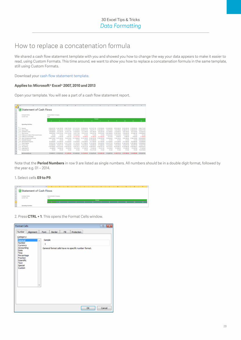
How to replace a concatenation formulaWe shared a cash flow statement template with you and showed you how to change the way your data appears to make it easier to read, using Custom Formats. This time around, we want to show you how to replace a concatenation formula in the same template, still using Custom Formats.

Download your cash flow statement template.


Open your template. You will see a part of a cash flow statement report.

Note that the Period Numbers in row 9 are listed as single numbers. All numbers should be in a double digit format, followed by the year e.g. 01 – 2014.

1. Select cells E9 to P9.

2. Press CTRL + 1. This opens the Format Cells window.

http://www.sagedl.com/sage-email/PDFs/Cashflow%20Statement%20-%20Text%20Custom%20Formats.xlsx

30


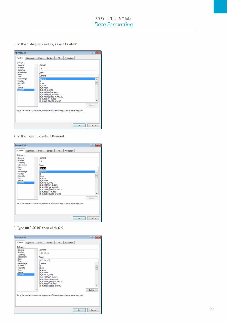
3. In the Category window, select Custom.

4. In the Type box, select General.

5. Type 00 “ -2014” then click OK.

31


The period values have now been adjusted to a two-digit format to represent the period, and are appended with a “ – 2014” value.

While the same result could have been achieved by using a concatenation formula, this method of using Custom Formats removes the need for it. As it’s a format that will be saved in this workbook, it can be applied to other cells very easily.

32


Conditional Formatting using custom Excel formulas Conditional Formatting is an effective Microsoft® Excel® feature that allows you to highlight important information for example; the ability to find duplicate values within your spreadsheet. You can create your own rule by applying conditional formatting to cells or ranges of cells.

When you have selected the data you want to format, you can easily change the appearance of how your information is presented to help you easily analyze your data.



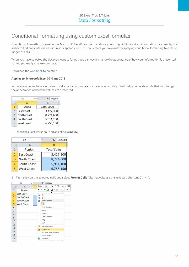
In this example, we have a number of cells containing values in excess of one million. We’ll help you create a rule that will change the appearance of how the values are presented.

1. Open the Excel workbook and select cells B2:B5.

2. Right click on the selected cells and select Format Cells (alternatively, use the keyboard shortcut Ctrl + 1).

http://www.sagedl.com/sage-email/PDFs/Conditional%20Syntax.xlsx

33


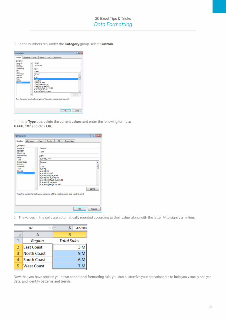
3. In the numbers tab, under the Category group, select Custom.

4. In the Type box, delete the current values and enter the following formula:#,###,, “M” and click OK.

5. The values in the cells are automatically rounded according to their value, along with the letter M to signify a million.

Now that you have applied your own conditional formatting rule, you can customize your spreadsheets to help you visually analyse data, and identify patterns and trends.

34


How to determine whether you are over or under budget, using custom formatsMonitoring budgets can be quite stressful and may involve the use of formulas. Instead of complicated formulas, you can use custom number formats within Microsoft® Excel® to easily determine if you are over or under budget.

All it takes are a few steps and you can then monitor your budget. Follow the steps below as we explain how:



1. Select the data range E4:E15 and right click on the selected range

2. Select Format Cells, then select Custom from the Category menu.

3. In the Type field select 0.

http://www.sagedl.com/sage-email/PDFs/How%20to%20quickly%20determine%20if%20over%20or%20under%20budget.xlsx

35


4. Type in the following: 0,000 “Under budget”;-0,000 “Over budget” Then select OK.

NB: If the formula populates an error, use the following instead: 0,000 “Under budget”;-0,000 “Over budget”

The values where the variance is positive have the words Under budget next to them. Where the variance is negative, Over budget is displayed. In that way it is easy to determine if a value is over or under budget.

36


How to quickly create a date format using a custom formula in ExcelBy adding a custom formula to a range of cells, you can create a date, without having to manually format each cell (this also known as suffixing numbers with text strings). Let’s say you have numbers in a spreadsheet and you wish to display them in a particular date format, you can apply a custom number formula to build a date range. Using this custom text string will help save you time and make your reports more reader friendly. In today’s tip we’ll show you how it can be done in four easy steps.



1. Select the data range D4:D20, and then right click.

2. Select Format Cells.

3. Select Custom from the Category box, and then select 0 under Type.

http://www.sagedl.com/sage-email/PDFs/24.06.2015_Suffix%20a%20number%20with%20a%20text%20string.xlsx

37


4. Enter the following: 0 “May 2015” under Type, then select OK.NB: Should your Excel settings differ, remove the spacing as follows: 0” May 2015”

Your selected data should now display the new date format as per below.

38


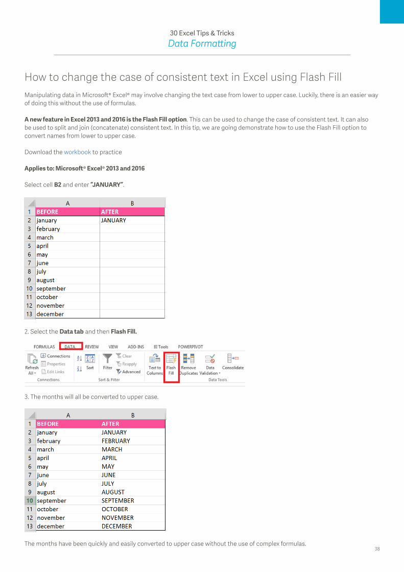
How to change the case of consistent text in Excel using Flash FillManipulating data in Microsoft® Excel® may involve changing the text case from lower to upper case. Luckily, there is an easier way of doing this without the use of formulas.

A new feature in Excel 2013 and 2016 is the Flash Fill option. This can be used to change the case of consistent text. It can also be used to split and join (concatenate) consistent text. In this tip, we are going demonstrate how to use the Flash Fill option to convert names from lower to upper case.



Select cell B2 and enter “JANUARY”.

2. Select the Data tab and then Flash Fill.

3. The months will all be converted to upper case.

The months have been quickly and easily converted to upper case without the use of complex formulas.

http://www.sagedl.com/sage-email/PDFs/How%20to%20change%20the%20case%20of%20consistent%20text.xlsx

39

30 Excel Tips & TricksPivotTables & PivotCharts

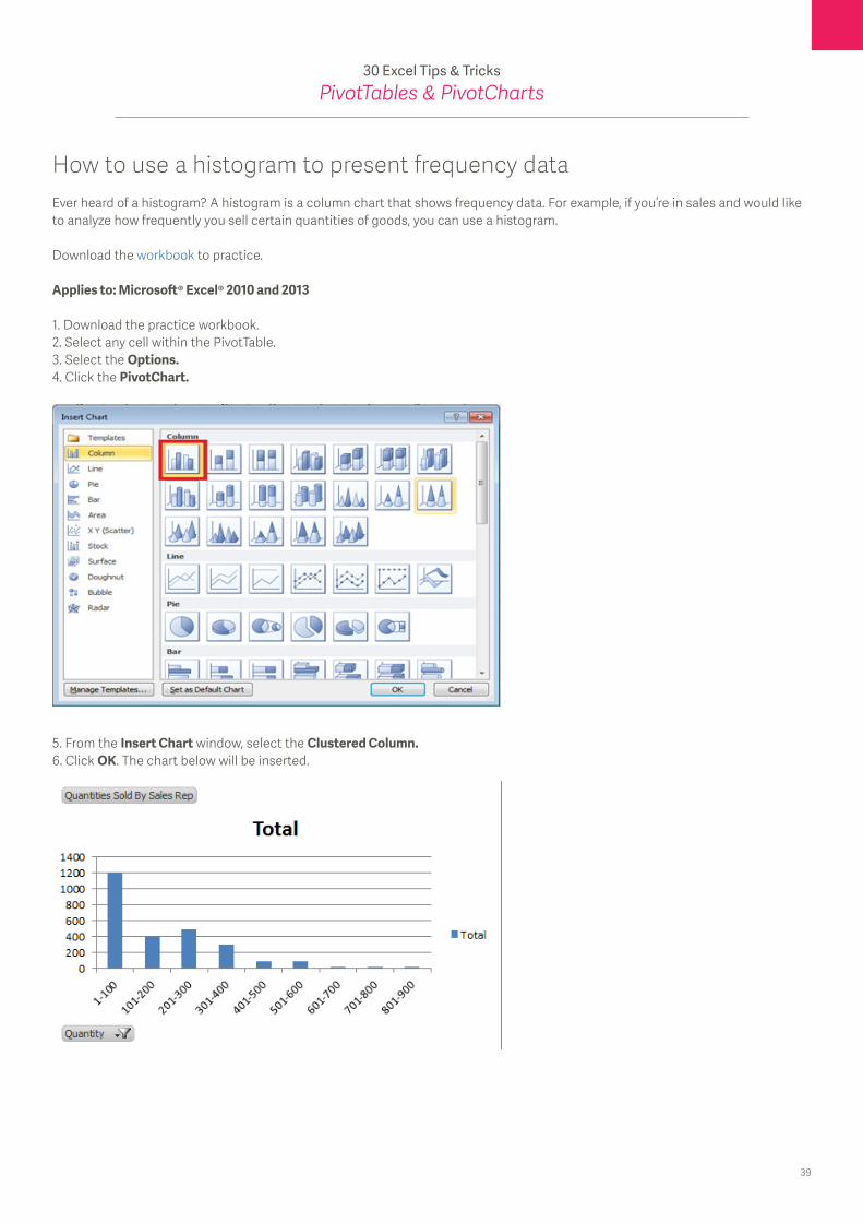
How to use a histogram to present frequency dataEver heard of a histogram? A histogram is a column chart that shows frequency data. For example, if you’re in sales and would like to analyze how frequently you sell certain quantities of goods, you can use a histogram.



1. Download the practice workbook.2. Select any cell within the PivotTable.3. Select the Options.4. Click the PivotChart.

5. From the Insert Chart window, select the Clustered Column.6. Click OK. The chart below will be inserted.

http://www.sagedl.com/sage-email/PDFs/Frequency%20of%20Quantities%20Sold.xlsx

40


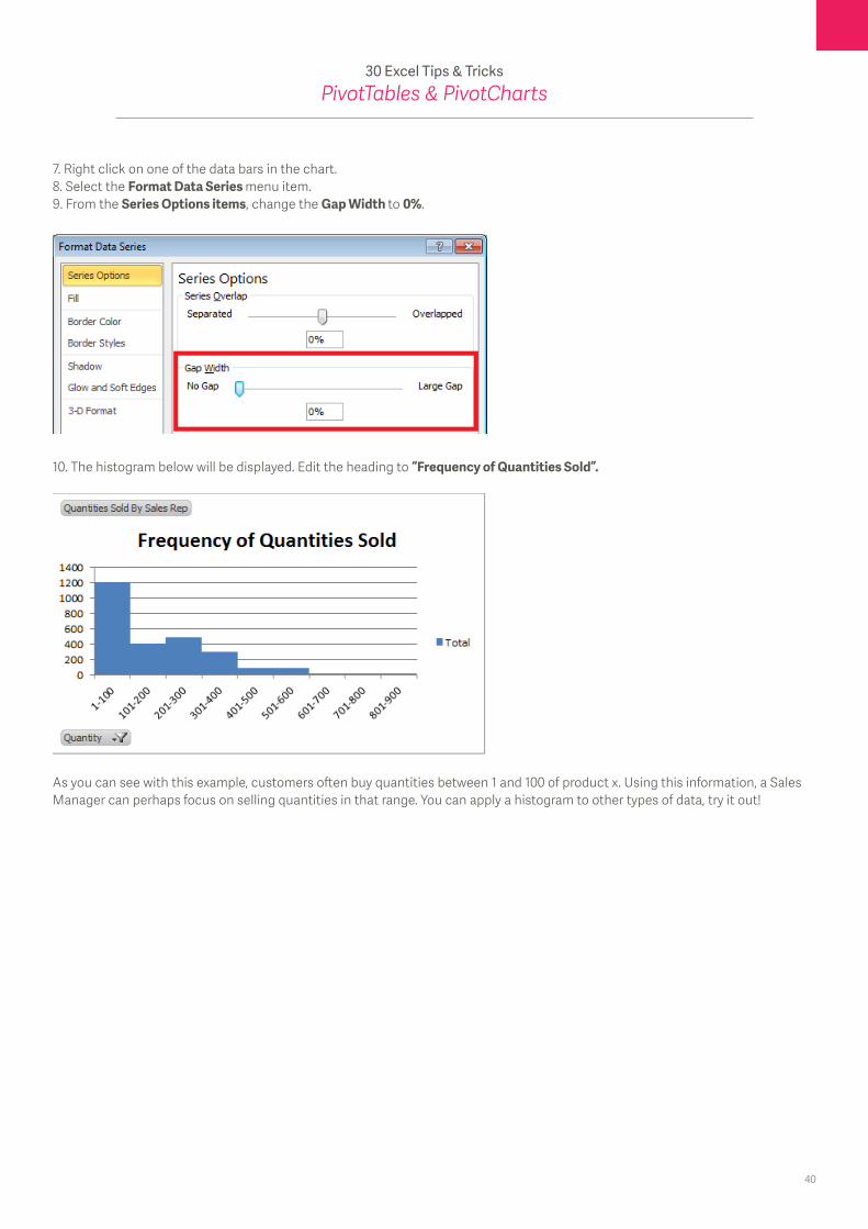
7. Right click on one of the data bars in the chart.8. Select the Format Data Series menu item.9. From the Series Options items, change the Gap Width to 0%.

10. The histogram below will be displayed. Edit the heading to “Frequency of Quantities Sold”.

As you can see with this example, customers often buy quantities between 1 and 100 of product x. Using this information, a Sales Manager can perhaps focus on selling quantities in that range. You can apply a histogram to other types of data, try it out!

41


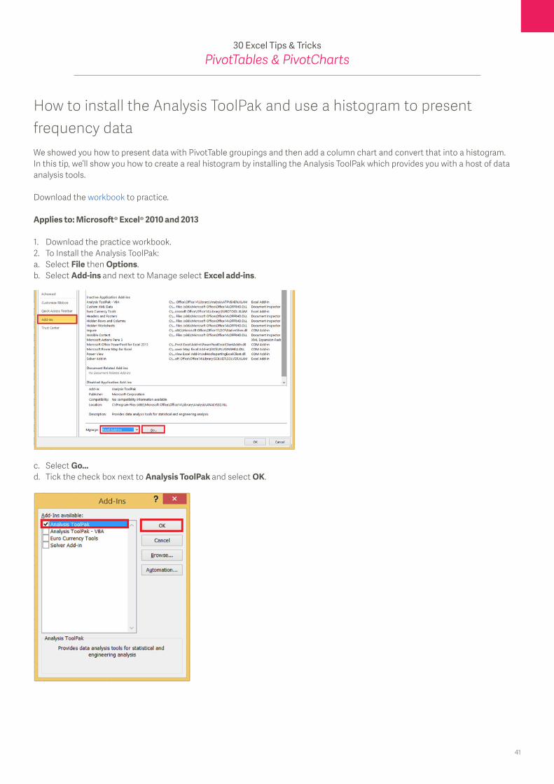
How to install the Analysis ToolPak and use a histogram to present frequency data We showed you how to present data with PivotTable groupings and then add a column chart and convert that into a histogram. In this tip, we’ll show you how to create a real histogram by installing the Analysis ToolPak which provides you with a host of data analysis tools.



1. Download the practice workbook.2. To Install the Analysis ToolPak:a. Select File then Options.b. Select Add-ins and next to Manage select Excel add-ins.

c. Select Go...d. Tick the check box next to Analysis ToolPak and select OK.

http://www.sagedl.com/sage-email/PDFs/How%20to%20use%20a%20histogram%20to%20present%20frequency%20data(Revisited).xlsx

42


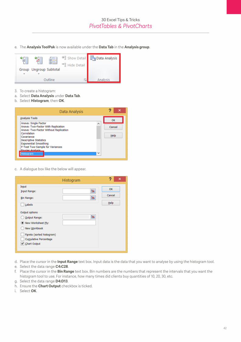
e. The Analysis ToolPak is now available under the Data Tab in the Analysis group.

3. To create a histogram:a. Select Data Analysis under Data Tab.b. Select Histogram, then OK.

c. A dialogue box like the below will appear.

d. Place the cursor in the Input Range text box. Input data is the data that you want to analyse by using the histogram tool.e. Select the data range C4:C28.f. Place the cursor in the Bin Range text box. Bin numbers are the numbers that represent the intervals that you want the histogram tool to use. For instance, how many times did clients buy quantities of 10, 20, 30, etc.g. Select the data range D4:D13.h. Ensure the Chart Output checkbox is ticked.i. Select OK.

43


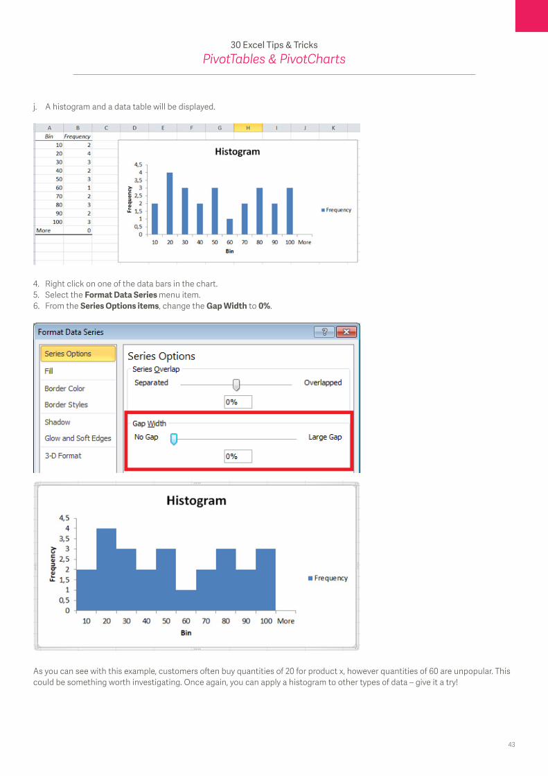
j. A histogram and a data table will be displayed.

4. Right click on one of the data bars in the chart.5. Select the Format Data Series menu item.6. From the Series Options items, change the Gap Width to 0%.

As you can see with this example, customers often buy quantities of 20 for product x, however quantities of 60 are unpopular. This could be something worth investigating. Once again, you can apply a histogram to other types of data – give it a try!

44


How to create a waterfall chartA waterfall chart, which is a special type of a column chart, is normally used for understanding how an initial value is affected by a series of intermediate positive or negative values. Usually the initial and the final values are represented by whole columns, while the intermediate values are denoted by floating columns.

In this tip we show you how to create a waterfall chart.

Download the dashboard template to practice.


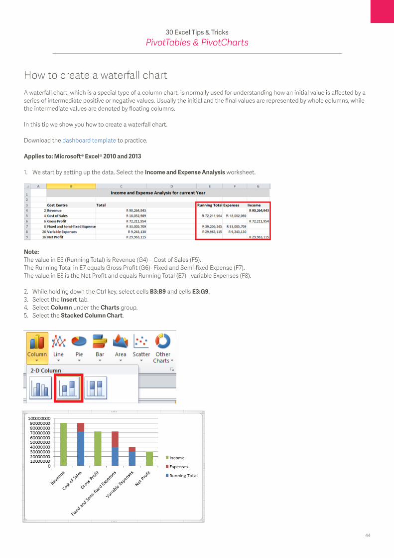
1. We start by setting up the data. Select the Income and Expense Analysis worksheet.

Note:The value in E5 (Running Total) is Revenue (G4) – Cost of Sales (F5).The Running Total in E7 equals Gross Profit (G6)- Fixed and Semi-fixed Expense (F7).The value in E8 is the Net Profit and equals Running Total (E7) - variable Expenses (F8).

2. While holding down the Ctrl key, select cells B3:B9 and cells E3:G9.3. Select the Insert tab.4. Select Column under the Charts group.5. Select the Stacked Column Chart.

http://www.sagedl.com/sage-email/PDFs/FinancialDashboardTemplate_Waterfall%20chart.xlsm

45


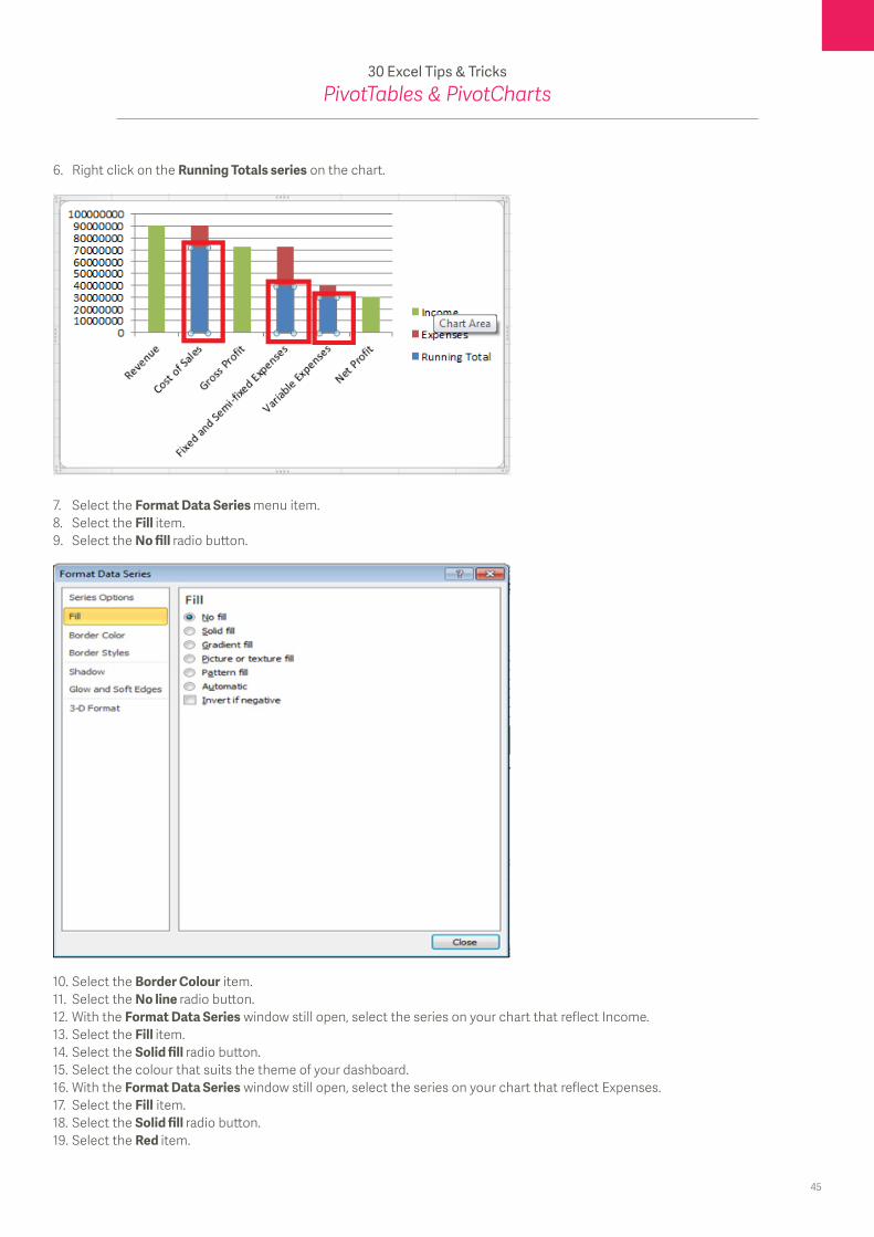
6. Right click on the Running Totals series on the chart.

7. Select the Format Data Series menu item. 8. Select the Fill item. 9. Select the No fill radio button.

10. Select the Border Colour item. 11. Select the No line radio button. 12. With the Format Data Series window still open, select the series on your chart that reflect Income. 13. Select the Fill item. 14. Select the Solid fill radio button. 15. Select the colour that suits the theme of your dashboard. 16. With the Format Data Series window still open, select the series on your chart that reflect Expenses. 17. Select the Fill item. 18. Select the Solid fill radio button. 19. Select the Red item.

46


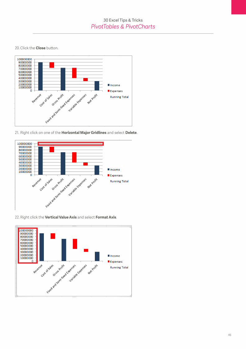
20. Click the Close button.

21. Right click on one of the Horizontal Major Gridlines and select Delete.

22. Right click the Vertical Value Axis and select Format Axis.

47


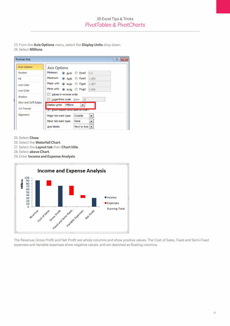
23. From the Axis Options menu, select the Display Units drop down.24. Select Millions.

25. Select Close.26. Select the Waterfall Chart.27. Select the Layout tab then Chart title.28. Select above Chart.29. Enter Income and Expense Analysis.

The Revenue, Gross Profit and Net Profit are whole columns and show positive values. The Cost of Sales, Fixed and Semi-Fixed expenses and Variable expenses show negative values, and are depicted as floating columns.

48


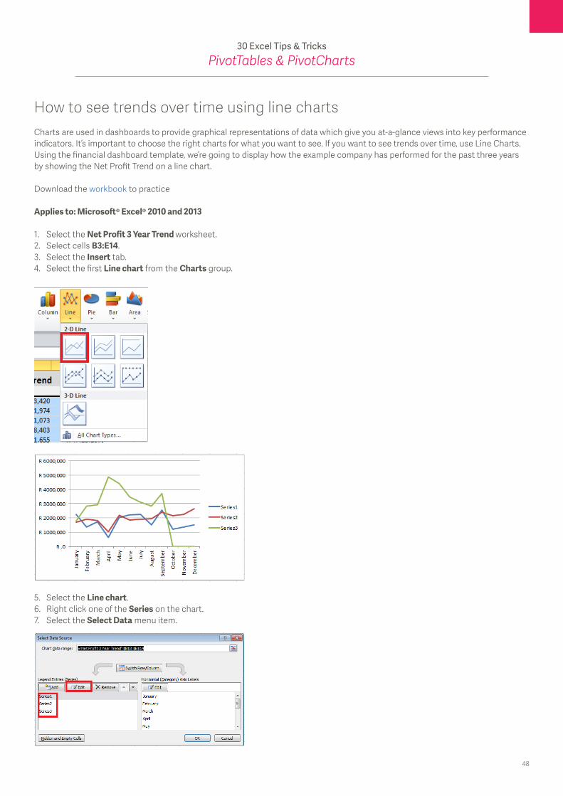
How to see trends over time using line charts Charts are used in dashboards to provide graphical representations of data which give you at-a-glance views into key performance indicators. It’s important to choose the right charts for what you want to see. If you want to see trends over time, use Line Charts. Using the financial dashboard template, we’re going to display how the example company has performed for the past three years by showing the Net Profit Trend on a line chart.



1. Select the Net Profit 3 Year Trend worksheet.2. Select cells B3:E14.3. Select the Insert tab.4. Select the first Line chart from the Charts group.

5. Select the Line chart.6. Right click one of the Series on the chart.7. Select the Select Data menu item.

http://www.sagedl.com/sage-email/PDFs/FinancialDashboardLineChart.xlsx

49


8. From the Select Data Source window, select Series1 and click the Edit button under Legend Entry Series. 9. Place your cursor in the Series Name box.

10. On the Net Profit 3 Year Trend worksheet, select cell C2. Click OK. 11. From the Select Data Source window, select Series2 and click the Edit button under Legend Entry Series. 12. Place your cursor in the Series Name box. 13. On the Net Profit 3 Year Trend worksheet, select cell D2. Click OK. 14. From the Select Data Source window, select Series3 and click the Edit button under Legend Entry Series. 15. Place your cursor in the Series Name box. 16. On the Net Profit 3 Year Trend worksheet, select cell E2. Click OK. 17. Click the OK button to exit from the Select Data Source window.

18. Right click on one of the Horizontal Axis Major Gridlines and select Delete. 19. Right click the Horizontal Category Axis and select the Font menu item. 20. Change the font size in the Size box to 7. Click OK.

50


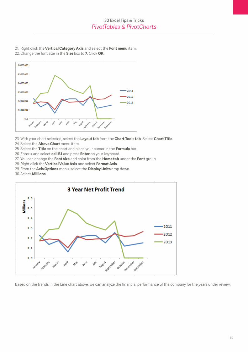
21. Right click the Vertical Category Axis and select the Font menu item. 22. Change the font size in the Size box to 7. Click OK.

23. With your chart selected, select the Layout tab from the Chart Tools tab. Select Chart Title. 24. Select the Above Chart menu item. 25. Select the Title on the chart and place your cursor in the Formula bar. 26. Enter = and select cell B1 and press Enter on your keyboard.27. You can change the Font size and color from the Home tab under the Font group. 28. Right click the Vertical Value Axis and select Format Axis.29. From the Axis Options menu, select the Display Units drop down.30. Select Millions.

Based on the trends in the Line chart above, we can analyze the financial performance of the company for the years under review.

51


5 Easy steps to create a PivotChart in ExcelYou can easily represent your data from a PivotTable into a PivotChart. PivotCharts allow you to graphically represent your data which can help you to easily see comparisons, patterns and trends. For example, a Sales Manager can use PivotCharts to analyse the performance of his or her sales staff.

A PivotTable is an interactive table that summarises large amounts of data, which you can analyse even further using a PivotChart. Instead of creating a regular chart from scratch each time, you can create a single PivotChart and view different parts of your data by changing your PivotTable.

You can create a Pivot Chart from scratch or from an existing PivotTable. In this week’s tip we’ll show you how to create a PivotChart from scratch.


1. Select any cell within the data range.2. Select the Insert tab then Pivot Chart. Then select OK.

3. Drag and place the Sales Persons field into the axis field’s area (categories).4. Drag and place the Product Sales fields into the values area.

5. Add a title to the chart.a. Select the chart.b. Select the layout tab.c. Select chart title.d. Select above chart.e. Enter the title, Sales Report.

f. The chart will be displayed as below.

http://www.sagedl.com/sage-email/PDFs/15.10.2015_How%20to%20create%20a%20Pivot%20Chart.xlsx

52


As you can see, you have now created an interactive PivotChart, using the data in your PivotTable.

A PivotChart report always has an associated PivotTable report. Both reports have fields that correspond to each other. When you change the position of a field in one report, the corresponding field in the other report also moves.

53


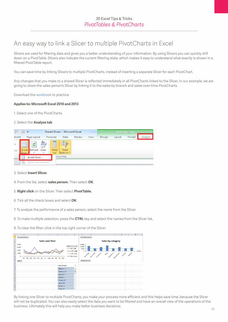
An easy way to link a Slicer to multiple PivotCharts in ExcelSlicers are used for filtering data and gives you a better understanding of your information. By using Slicers you can quickly drill down on a PivotTable. Slicers also indicate the current filtering state, which makes it easy to understand what exactly is shown in a filtered PivotTable report.

You can save time by linking Slicers to multiple PivotCharts, instead of inserting a separate Slicer for each PivotChart.

Any changes that you make to a shared Slicer is reflected immediately in all PivotCharts linked to the Slicer. In our example, we are going to share the sales person’s Slicer by linking it to the sales-by-branch and sales-over-time PivotCharts.



1. Select one of the PivotCharts.

2. Select the Analyze tab.

3. Select Insert Slicer.

4. From the list, select sales person. Then select OK.

5. Right click on the Slicer. Then select PivotTable.

6. Tick all the check boxes and select OK.

7. To analyze the performance of a sales person, select the name from the Slicer.

8. To make multiple selection: press the CTRL key and select the names from the Slicer list.

9. To clear the filter: click in the top right corner of the Slicer.

By linking one Slicer to multiple PivotCharts, you make your process more efficient and this helps save time, because the Slicer will not be duplicated. You can also easily select the data you want to be filtered and have an overall view of the operations of the business. Ultimately this will help you make better business decisions.

http://www.sagedl.com/sage-email/PDFs/22.10.2015_Shared%20Slicers.xlsx

54

30 Excel Tips & TricksKeyboard Shortcuts

Search for and delete rows with duplicate data in two easy stepsIf you have a worksheet with a lot of data and you want to ensure your data integrity, you need to make certain that there are no duplicates in your data. Trying to find and remove duplicates in your worksheet can be like trying to find a needle in a haystack. Fortunately, the Remove Duplicates dialog box makes it easy and quick for you, and it’s even quicker when you use keyboard shortcuts.



1. Open the demonstration workbook. Note that there are four rows highlighted. The yellow row is the original data row, and the three blue rows are duplicates of that row.

2. Press ALT + A, M This will launch the Remove Duplicates dialogue box.

To determine which rows have duplicate data, Excel searches data in columns. And, by default, the Remove Duplicates dialogue box opens with all column headings checked/ticked. In this case, since we want to remove rows that have the exact same data, we will leave all column headings checked.

http://www.sagedl.com/sage-email/PDFs/Demo%20Data%20-%20Delete%20Duplicate%20Rows.xlsx

55


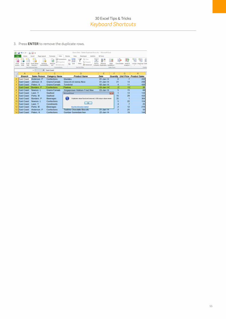
3. Press ENTER to remove the duplicate rows.

56


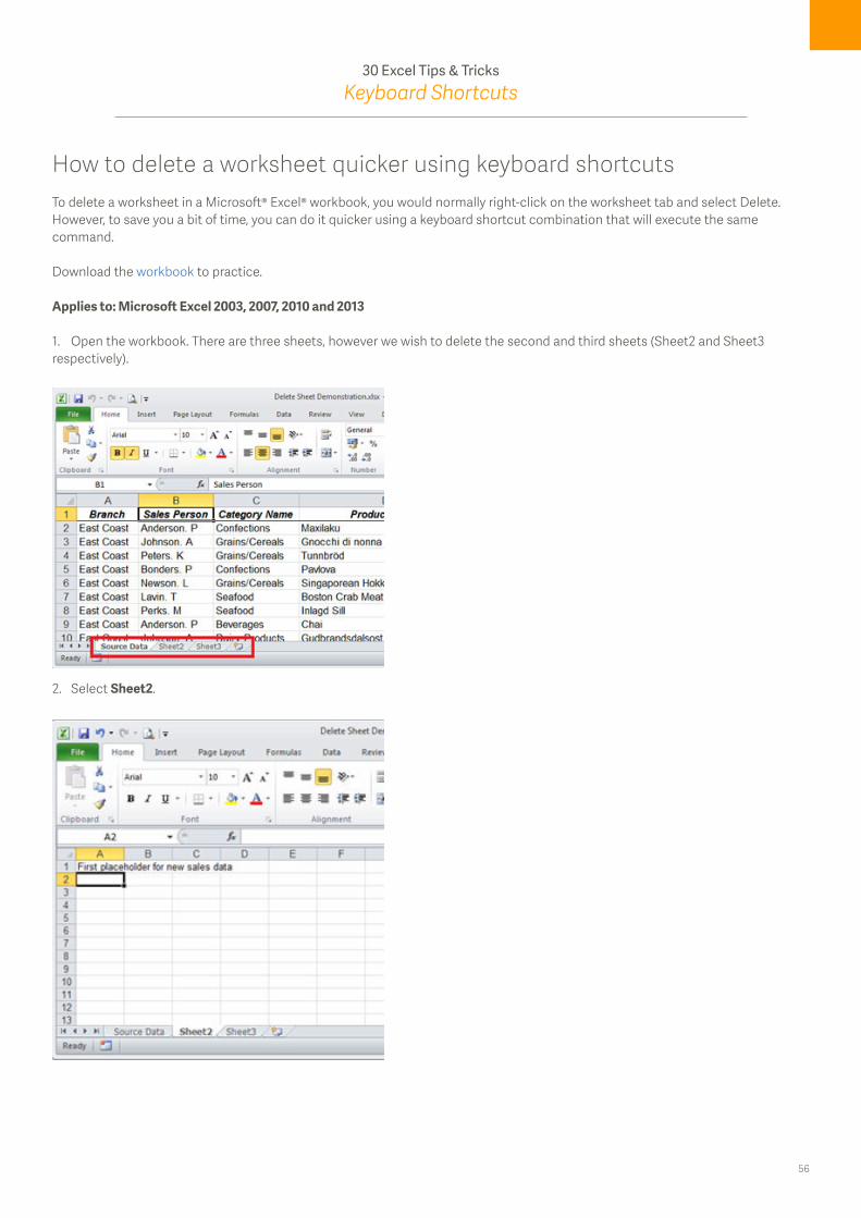
How to delete a worksheet quicker using keyboard shortcutsTo delete a worksheet in a Microsoft® Excel® workbook, you would normally right-click on the worksheet tab and select Delete. However, to save you a bit of time, you can do it quicker using a keyboard shortcut combination that will execute the same command.


Applies to: Microsoft Excel 2003, 2007, 2010 and 2013

1. Open the workbook. There are three sheets, however we wish to delete the second and third sheets (Sheet2 and Sheet3 respectively).

2. Select Sheet2.

http://www.sagedl.com/sage-email/PDFs/Delete%20Sheet%20Demonstration.xlsx

57


3. Press ALT + E, then the L key.

4. Select Delete in the Confirm Deletion window. The sheet will now be deleted.

5. Sheet3 will now be selected. Press F4 to repeat your last command, and you will be able to delete this sheet as well.The F4 keyboard shortcut repeats the last command. This shortcut will also apply if you chose to use the right-click method deletion method.

Additional Note: Microsoft Excel 2010 and 2013 have a new keyboard shortcut for deleting a sheet – Alt + H, D, S. However, they will still recognise the original version, which involves one less keystroke.

58


How to expand and collapse grouped columns using keyboard shortcutsGrouped columns and rows (sometimes called Outline Data) are an alternative for hiding and showing data without using the Hide and Unhide function. Both options are great for organizing and de-cluttering worksheets which have a lot of data on display. Did you know that you can expand and collapse grouped columns using keyboard shortcuts? Follow the steps below to see how:



1. Open the exercise workbook. You will see that three columns (B, C and D) are grouped together.

2. Select any cell in those three columns then press ALT, A, H.

The grouped rows are now in a collapsed view.

http://www.sagedl.com/sage-email/PDFs/Demo%20-%20Expand%20and%20Collapse%20Grouped%20Columns.xlsx

59


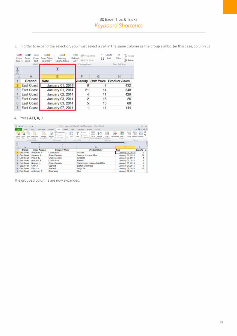
3. In order to expand the selection, you must select a cell in the same column as the group symbol (in this case, column E).

4. Press ALT, A, J.

The grouped columns are now expanded.

60


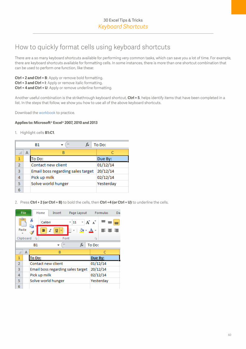
How to quickly format cells using keyboard shortcutsThere are a so many keyboard shortcuts available for performing very common tasks, which can save you a lot of time. For example, there are keyboard shortcuts available for formatting cells. In some instances, there is more than one shortcut combination that can be used to perform one function, like these:

Ctrl + 2 and Ctrl + B: Apply or remove bold formatting. Ctrl + 3 and Ctrl + I: Apply or remove italic formatting. Ctrl + 4 and Ctrl + U: Apply or remove underline formatting.

Another useful combination is the strikethrough keyboard shortcut, Ctrl + 5, helps identify items that have been completed in a list. In the steps that follow, we show you how to use all of the above keyboard shortcuts.



1. Highlight cells B1:C1.

2. Press Ctrl + 2 (or Ctrl + B) to bold the cells, then Ctrl +4 (or Ctrl + U) to underline the cells.

http://www.sagedl.com/sage-email/PDFs/Format%20Cells%20-%20Part%201%20-%20Strikethrough.xlsx

61


3. Highlight cells B2:B4.

4. Press Ctrl + 5 to apply strikethrough formatting to all cells.

62

30 Excel Tips & TricksAdditional Learning

This e-book is a just taste of how we can teach you to use Excel smarter. We also offer a unique training course, Excel on Steroids, which focuses on Excel features for business reporting.

How will the Excel on Steroids course benefit you?The course will help you become more efficient in using Excel for business reporting so you can:• Save time• Increase your productivity and improve your performance• Enhance your Excel reporting skills• Better decision making through improved report presentation and analysis

Excel on Steroids is offered classroom-based in South Africa for Microsoft Excel 2007, 2010 and 2013. It is also offered online on the Sage Intelligence Academy for Microsoft Excel 2010 and 2013.

• For queries on classroom-based training in South Africa, get in touch with us.• For online training, visit the Sage Intelligence Academy.

For further information, please visit our website: https://www.sageintelligence.com/training/excel-on-steroids/

Sage Intelligence is a flexible Business Intelligence (BI) reporting tool that gives you the freedom to design reports according to your business’s unique requirements. And it’s built in Microsoft® Excel®, a tool you’re already familiar with.

Sage Intelligence Tips and Tricks are published twice a month, and Sage Intelligence Tips and Tricks e-books are available for you to download at no cost.

Subscribe

Learnt handy tips and tricks in this e-book? Learn how to use Excel even smarter!

Subscribe to our Sage Intelligence tips and tricks

http://www.sageintelligenceacademy.com/SignifyHR_Sage/Projects2/LearningStore

mailto:mailto:training.sales2%40sage.com?subject=I%20would%20like%20more%20info%20on%20classroom-based%20training%20please

http://www.sageintelligenceacademy.com/SignifyHR_Sage/Projects2/LearningStore

https://www.sageintelligence.com/subscribe/si/

Documents

30 Microsoft®Excel® Tips and Tricks - RKL eSolutions, LLC · PDF file30 Microsoft®Excel® Tips and Tricks Microsoft Excel 2007, 2010 & 2013 Functions & Formulas PivotTables & PivotCharts