Advanced Course on

Communication in Networks

Friedhelm Meyer auf der Heide

Heinz Nixdorf Institute &

Faculty for Computer Science,

Electrical Engineering,

and Mathematics

Contents

1 Routing 3

1.1 A simple example . . . . . . . . . . . . . . . . . . . . . . . . . . . . . . . . 4

2 Some networks and path systems 6

2.1 Adaptive Path Selection in (n, d)-PN and M(n, d) . . . . . . . . . . . . . . 8

3 Oblivious path selection in the hypercube 10

4 Offline Switching 13

4.1 Probabilistic Methods . . . . . . . . . . . . . . . . . . . . . . . . . . . . . 13

4.2 Offline Switching . . . . . . . . . . . . . . . . . . . . . . . . . . . . . . . . 14

5 Online Switching 18

5.1 A Switching Protocol for Directed Acyclic Graphs . . . . . . . . . . . . . . 18

5.2 Analysis of the Switching Protocol . . . . . . . . . . . . . . . . . . . . . . 18

2

Overview

This course describes some advanced topics from the theory of communication in networks.We will deal with

- Routing in networks

- Scheduling jobs in distributed systems

- Data management in networks.

My lecture notes on ”Kommunikation in parallelen Rechenmodellen” form a basis for thislecture; part of the material is adapted from the lecture notes ”Communication in parallelsystems” by Christian Scheideler.

1 Routing

A network is described by a set P = {P1, . . . , Pn} of processors and an undirected graphG = (P , E). E contains the edges or links. Each processor has a buffer of some size B foreach incident edge. Such a buffer can store B packets. Two processors Pi, Pj can directlycommunicate, if they are connected by a link. In this case Pi can send a packet to Pj inone step.

If Pi and Pj are not connected by a link, they have to choose a routing path, i.e., a pathfrom Pi to Pj in G, and to send the packet from vertex to vertex along this path. We willnow define the routing problem in some more detail.

A packet contains data, its source s ∈ P , its destination d ∈ P , and possibly some moreinformation for the routing.

A routing problem is described by a set S = {(si, di), i = 1, . . . ,m} of source-destinationpairs.

Routing according to S means to send a packet from si to di, for each i = 1, . . . ,m.

We will always distinguish between two parts of the routing process:

- path selection: How are the paths in G selected that connect the sources with theirdestinations?

- packet switching: How does a node decide which of the packets it currently stores tomove next? This implies the decision, when a node injects a packet into the system.

If the paths wi are fixed for each source destination pair (si, di) ∈ S, the following param-eters are well defined:

• the dilation D (of S in G), i.e., the maximum length of the routing paths used.

3

• the congestion C (of S in G), i.e., the maximum number of routing paths that sharethe same edge.

It is easily seen that

- max{D,C} is a lower bound for the routing time,

- D · C is an upper bound for the routing time,

- C is an upper bound on the buffer size.

A routing strategy proceeds in rounds.

In a round, each node can choose, for each outgoing edge, a packet from the buffers ofthe incoming edges, and move it along the edge to the respective buffer of the neighboringnode. In addition it can inject a new packet into the system.

The choice of the packets to be moved next is done by the routing (or switching) protocol,the decision, which packet to move along which edge is done by the path selection. Therouting time needed for a routing problem S is the number of rounds needed until allpackets have reached their destinations.

We will distinguish between different types of routing strategies:

- oblivious versus adaptive. Routing is called oblivious, if each routing path is chosensolely dependent on its source and its destination. In case of a dependence of thechoices (which is reasonable in order to reduce congestion) we deal with adaptiverouting.

- online versus offline. Routing is called online, if initially each node only knows thepackets it injects into the system, but no further packets. (It may know the networktopology and the selected paths in case of oblivious routing). Thus the switchingprotocol is based only on local information.

If global information about the routing problem can be used for the switching protocoland/or the path selection, we talk about adaptive routing.

1.1 A simple example

Consider the ring of length n consisting of n nodes [n] (=: {0, . . . , n − 1}), and edges{{i, i+ 1}, i ∈ [n− 1]} ∪ {{n− 1, 0}}.Permutation routing can easily be done in time bn

2c, because no collisions occur, and the

ring has diameter bn2c.

Now consider an arbitrary routing problem S of size m. How long does it take? If allm packets have to be sent from 0 to bn

2c, obviously time m + bn

2c − 1 is necessary and

sufficient. Can we route every problem of size m within this time bound? Yes!

4

Consider the following routing strategy: Our path system consists of the shortest paths.(Note: These paths have length at most bn

2c.) Our switching role is furthest-to-go (FTG):

If packets contend to use the same link in the same direction at the same time, the onethat still has the longest path to its destination is preferred. In case of a tie, the one withmaximum index wins.

Theorem 1.1 Every routing problem of size m on the ring of length n can be solved intime at most m+ bn

2c − 1.

Proof. Let P = (p1, . . . , pm) denote the set of all packets, and let the rank rankv(pi) ofpacket pi at node v be defined as the number of edges pi still has to traverse from v plusi/(m+1). According to our preference rules it must hold for any two packets p, q at somenode v where p is preferred against q that

rankv(p) > rankv(q) .

We will need this observation later.

Now, let us use a proof method called backwards analysis. We start with the last packet thatreached its destination. Let this packet be called q1 ∈ {p1, . . . , pm}, and let its destinationbe called v0. We follow q1 backwards in time till it was delayed by some other packet, sayq2, at some node v1. Let `1 be the number of edges traversed from v0 to v1. We continueto follow q2 backwards in time until it was delayed by some other packet, say q3, at somenode v2. Let `2 be the number of edges traversed from v1 to v2. In general, we will followpacket qi backwards in time until it was delayed by some other packet, say qi+1, at somenode vi. Let `i be the number of edges traversed from vi−1 to vi. If we reach a packet qithat has not been delayed by any other packet, we simply follow it backwards in time untilit reached its source node, called vi.

Assume now that we touched s packets q1, . . . , qs in the course of this argument. Usingour observation above, we can state the following three facts:

1. rankv0(q1) ≥ 0

2. rankvi(qi+1) > rankvi(qi)

3. rankvi(qi) = rankvi−1(qi) + `i

We will use these facts to prove the following lemmas.

Lemma 1.2∑s

i=1 `i ≤ bn/2c.

Proof. A straightforward induction argument shows that the above facts imply rankvk(qk) ≥∑k

i=1 `i for every k ∈ {1, . . . , s}. However, since rankvs(qs) must be smaller than bn/2c+1due to a maximum path length of bn/2c we get

bn/2c+ 1 > rankvs(qs) ≥k∑

i=1

`i

5

which yields the lemma since the `i are integers. ¤

Lemma 1.3 s ≤ m

Proof. Due to fact (2) and the fact that if rankv(p) > rankv(q) for two packets p andq then this relationship also holds for all other nodes visited by p and q, it holds that nopacket can appear more than once in the backwards argument. Hence, s ≤ m. ¤

Obviously, the total runtime of our strategy is equal to the time covered by the backwardsargument. Since the number of time steps covered by this argument is exactly

∑si=1 `i +

s− 1, the two lemmas above imply a runtime of at most

bn/2c+m− 1 .

¤

Theorem 1.1 is worst case optimal, since a routing problem can easily be set up thatrequires m+ bn/2c − 1 steps.

2 Some networks and path systems

We present some basic networks and some of their properties.

• (n, d)-meshes.

Let n, d be positive integers. The (n, d)-mesh M(n, d) has nodes [n]d (note: [n] :={0, . . . , n−1}). {a, b} ∈ E, iff |a− b| = 1, i.e., a and b differ in exactly one coordinatei, and |ai − bi| = 1.

Some properties of M(n, d) :

– size: N = nd.

– diameter: d · (n− 1) = d · (N 1d − 1).

– degree: 2d.

– a simple path system:

dimension order paths, i.e. path from (a1, . . . , ad) to (b1, . . . , bd) goes:(a1, . . . , ad)→ (b1, a2, . . . , ad)→ (b1, b2, a3, . . . , ad)→ . . . (b1, . . . , bd).

These paths are shortest paths. But even for permutation routing, we get highcongestion.

Example: Reversal permutation: (a1, . . . , ad)→ (ad, ad−1, . . . , a1).

All packets with sources (0, . . . , 0, ad/2, . . . , ad) go through (0, . . . , 0), thus con-

gestion ≥√N . (We will later see that no path system has better worst case

congestion for permutations in the mesh).

6

100010 110001 101011000 111

−3

−2

−1

1

2

3

sources

sinks

(a) (2, 3)-PN

000 100010 110001 101011 111

1

2

3

0

(b) BF(3)

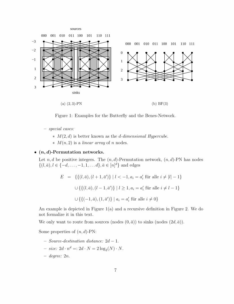
Figure 1: Examples for the Butterfly and the Benes-Network.

– special cases:

∗ M(2, d) is better known as the d-dimensional Hypercube.

∗ M(n, 2) is a linear array of n nodes.

• (n, d)-Permutation networks.

Let n, d be positive integers. The (n, d)-Permutation network, (n, d)-PN has nodes{(l, a), l ∈ {−d, . . . ,−1, 1, . . . d}, a ∈ [n]d} and edges

E = {{(l, a), (l + 1, a′)} | l < −1, ai = a′i fur alle i 6= |l| − 1}

∪ {{(l, a), (l − 1, a′)} | l ≥ 1, ai = a′i fur alle i 6= l − 1}

∪ {{(−1, a), (1, a′)} | ai = a′i fur alle i 6= 0}

An example is depicted in Figure 1(a) and a recursive definition in Figure 2. We donot formalize it in this text.

We only want to route from sources (nodes (0, a)) to sinks (nodes (2d, a)).

Some properties of (n, d)-PN:

– Source-destination distance: 2d− 1.

– size: 2d · nd =: 2d ·N = 2 log2(N) ·N .

– degree: 2n.

7

– path selection: see Section 2.1

– special cases:

∗ Benes- Network: (2, d)-PN (Figure 1)

∗ Butterfly: upper half of (2, d)-PN (Figure 1)

2.1 Adaptive Path Selection in (n, d)-PN and M(n, d)

Our first goal is to find disjoint paths in (n, d)-PN connecting source a to destinationΠ(a), a ∈ [n]d, for arbitrary permutations Π. To do so, we need some prerequisities fromgraph theory.

Let G = (V,E) be an undirected graph (multiple edges allowed). M ⊆ E is a matchingin G, if no two edges in M are incident, i.e., share a vertex. M is a perfect matching, if itcovers all vertices of G. f : E → {1, . . . , k} is a k-coloring of G, if incident edges e, e′ fulfilf(e) 6= f(e′) (i.e., have different colors).

Note: Each color-class E` = {e ∈ E, f(e) = `} forms a matching.

For a set S ⊆ V,Γ(S) denotes {u ∈ V \ S,∃{u, v} ∈ E with u ∈ S}. (Γ(S) is theneighbourhood of S in G.)

Theorem 2.1 (Hall’s Theorem)Let G = (V1∪V2, E) be bipartite, |V1| = |V2|. Then: G contains a perfect matching, if andonly if, for each S ⊆ V1, |Γ(S)| ≥ |S|. ¤

(For a proof, see Script “Kommunikation in parallelen Rechenmodellen”.)

Corollary 2.2 (Coloring Theorem)Each bipartite graph of degree c is c-colorable. ¤

We now are ready to state our first result.

Theorem 2.3 For every permutation Π on [n]d there are disjoint paths wa, a ∈ [n]d oflengths 2d− 1 such that wa connects source a with destination Π(a) of (n, d)-PN.

Proof: We will construct these paths inductively on d. (see Figure 2 for the recursivedecomposition of (n, d)-PN.)

d = 1:

In this case the paths are just edges in the complete bipartite graph (n, 1)-PN.

d > 1:

Note: We may direct wa through any of the n subnetworks B(0), . . . , B(n−1) of (n, d)-PN.If we choose some B(i), then the source and the destination of B(i) used by wa are unique.Our goal now is to choose a B(i) for each wa such that

8

d = 1: 0 1 −1n

0 1 −1n

d ≥ 2:

n,d( −1) PNn,d( −1) n,d( −1)

B B B(1)(0) ( )n−1PN- PN- -

Figure 2: Recursive Construction of (n, d)-PN.

(∗) every source and every destination of every B(i) is used by exactly one wa.

If we find such an assignment of paths to the B(i)’s, then we are left with a permuta-tion routing problem in each B(i). For these problems, disjoint paths exist by inductionhypothesis.

Thus all we have to do is to assign paths to B(i)’s, such that (∗) holds. For this we considerGΠ, the collision graph of Π in (n, d)-PN: GΠ is bipartite, its nodes are [n]d−1∪[n]d−1,representing the sources and destinations of B(0), resp.

{a, b} is an edge of GΠ, if there are i, j ∈ [n] such that Π(ia) = jb, i.e., the path wia, whendirected through B(0), enters B(0) at source a and leaves it at destination b.

By construction GΠ has degree n. Thus, by Theorem 2.2, GΠ is n colorable.

Let Wi denote the set of paths wa defining an edge in GΠ with color i. Direct these pathsthrough B(i). As the edges of GΠ defined by the paths in Wi form a matching, the aboveassignment fulfils property (∗)Thus, by the discussion above, we can proceed inductively to construct the desired disjointpaths.

¤

An immediate consequence of Theorem 2.3 is the following.

Theorem 2.4 Offline adaptive permutation routing in (n, d)-PN can be done in time 2d−1. ¤

We now will see that the some techniques also yield efficient permutation routing inM(n, d).

Theorem 2.5 Offline, adaptive permutation routing in M(n, d) can be done in time 2(n−1)d.

(Note that this is only by a factor 2 away from the diameter bound.)

Proof. We again argue inductively w. r. t. d.

9

d = 1:

On a linear array we can route permutations in time 2(n− 1).

d > 1:

We partition M(n, d) in n copies M (0), . . . ,M (n−1) of M(n, d− 1). Now consider the samegraph GΠ with vertex set [n]d−1∪[n]d−1 as in the previous proof.

By this, each packet pa, a ∈ [n]d is assigned a color f(a) ∈ [n].

The 1D-source array of packet pia, i ∈ [n], a ∈ [n]d−1, is Aa = {0a, . . . , (n−1)a}. (Note: thisis a copy of M(n, 1)). The 1D-destination array of packet pb, b ∈ [n]d−1, is Aa, a ∈ [n]d−1

with Π(b) = ia for some i ∈ [n].

Now we are ready to state the routing protocol:

(i) for each a ∈ [n]d−1 in parallel: permute pia, i ∈ [n], i ∈ [n] on Aa such that pia reachesM f(ia),

(ii) recursively permute the packets in each M (i), such that each packet reaches its 1D-destination array,

(iii) permute each array Aa such that each packet reaches its destination. Note that,analogously to our discussion w. r. t. routing in (n, d)-PN, the routing problems in(i), (ii), (iii) are in fact permutation routing problems.

¤

3 Oblivious path selection in the hypercube

The following theorem demonstrates that no matter what kind of network and what kindof path system is used for oblivious routing, there is always a permutation that causes highcongestion.

Theorem 3.1 (Borodin/Hopcraft). Consider an arbitrary network G with n vertices anddegree d, and an arbitrary path system P in G. Then there is a permutation Π such thatrouting Π along paths from P causes congestion at least

√

nd. ¤

For the hypercube Hd this means that routing along the path system described in Section2, the so-called dimension-order routing, or along any other fixed path system, there is

always a permutation that causes congestion√

nlog(n)

, where n = 2d denotes the size of Hd.

(Note: Hd has degree d.)

We now show that this very large congestion can be avoided by introducing randomizationto the path system. We now apply the so-called Valiant’s trick:

Consider a fixed path system P in network G. The new path system is constructed asfollows: For each source-destination pair (s, d) choose randomly, uniformly, independently

10

an intermediate node v, and choose as path the concatenation of the paths from s to v andfrom v to d from P .

We apply this to the system P of dimension-order paths for the hypercube Hd. Thefollowing probabilities are w. r. t. these random choices of the intermediate nodes.

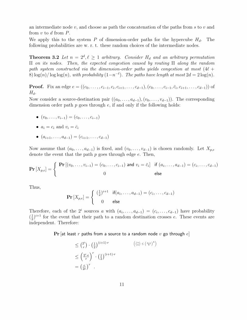
Theorem 3.2 Let n = 2d, ` ≥ 1 arbitrary. Consider Hd and an arbitrary permutationΠ on its nodes. Then, the expected congestion caused by routing Π along the randompath system constructed via the dimension-order paths yields congestion at most (4` +8) log(n)/ log log(n), with probability (1−n−`). The paths have length at most 2d = 2 log(n).

Proof. Fix an edge e = ((c0, . . . , , ci−1, ci, ci+1, . . . , cd−1), (c0, . . . , ci−1, ci, ci+1, . . . , cd−1)) ofHd.

Now consider a source-destination pair ((a0, . . . , ad−1), (v0, . . . , vd−1)). The correspondingdimension order path p goes through e, if and only if the following holds:

• (v0, . . . , vi−1) = (c0, . . . , ci−1)

• ai = ci and vi = ci

• (ai+1, . . . , ad−1) = (ci+1, . . . , cd−1)

Now assume that (a0, . . . , ad−1) is fixed, and (v0, . . . , vd−1) is chosen randomly. Let Xp,e

denote the event that the path p goes through edge e. Then,

Pr [Xp,e] =

{

Pr [(v0, . . . , vi−1) = (c0, . . . , ci−1) and vi = ci] if (ai, . . . , ad−1) = (ci, . . . , cd−1)

0 else

Thus,

Pr [Xp,e] =

{

(12)i+1 if(ai, . . . , ad−1) = (ci, . . . , cd−1)

0 else

Therefore, each of the 2i sources a with (ai, . . . , ad−1) = (ci, . . . , cd−1) have probability(12)i+1 for the event that their path to a random destination crosses e. These events are

independent. Therefore:

Pr [at least r paths from a source to a random node v go through e]

≤(

2i

r

)

·(

12

)(i+1)·r(

(

n

k

)

≤(

n·e

k

)

k)

≤(

2i·er

)r

·(

12

)(i+1)·r

=(

e2r

)r.

11

Since the hypercube has d2· 2d edges, we can conclude:

Pr [Congestion ≥ γd / log(d)]

≤ d2· 2d ·

(

e2γd/ log(d)

)γd/ log(d) (

d

2≤ 2d γ ≥ 2

)

≤ 22d ·(

dlog(d)

)−γd/ log(d) (

d

log(d)≥√d)

≤ 22d · d− 12γd/ log(d) = 22d · 2− 1

2γd

≤ 2(2− 12γ)d.

Thus, Pr[Congestion ≥ γd / log(d)] ≤ n−` for γ = 2`+ 4.

Thus, we have shown that routing a packet from each source node a to a random destinationv yields congestion at most (2` + 4) · d / log(d), with probability at least 1 − n−`. Now,given a permutation Π, the same argument holds for routing from random intermediatenodes to the destination nodes. Thus the Theorem follows. ¤

Thus we can achieve very low congestion for arbitrary permutations, with high probability.But we have to pay with non-optimal path length: Whereas shortest paths in Hd havelength at most d = log(n), we need paths up to length 2 log(n). Can we do better? Yes!Very recently, Berthold Vocking has presented a simple trick to do so:

For each source-destination pair a, b choose a random intermediate point v = (v0, . . . , vd−1)as above. Our Theorem yields congestion O(d/ log(d)), with high probability (w. h. p).

Now consider a second path system, where each intermediate note v is replaced by v =(v0, . . . , vd−1).

For each source destination pair now choose the shorter of the two paths in order to formthe randomized complemental path system.

Theorem 3.3 Each path in the randomized complemental paths system has length at mostd = log(n). Routing an arbitrary permutation along this path system causes congestionO(d / log(d)), w. h. p.

Proof. The congestion bound is clear, because, by the previous theorem, it even holds ifwe route Π along both path systems.

We have to check the path lengths. For a destination pair a, b with intermediate node v,the path length is h(a, v) + h(b, v), where h(., .) denotes the Hamming distance.

Note: h(a, v) = d− h(a, v) for all a, v ∈ {0, 1}d.Let p denote the path a→ v → b, p′ the path a→ v → b, |p| the length of path p.

Then: |p| = h(a, v) + h(b, v) = d− h(a, v) + d− h(b, v) = 2d− |p′|.Thus |p| or |p′| is at most d. ¤

12

4 Offline Switching

Suppose that a collection of simple (i.e. loop free) paths is given to us. Along each pathone packet has to be sent. All we know about the path collection is that is has a congestionof C and a dilation of D. In this case it is clear that at least max[C,D] steps are needed tosend the packets to their destinations. On the other hand, for any greedy method (everytime when at least one packet is waiting to traverse a link, this link forwards a packet) atmost C · D steps are needed. However, would it be also possible to send the packets totheir destinations in O(C +D) steps? We will investigate this problem in this section.

4.1 Probabilistic Methods

First, we introduce two methods that will be important for proving the existence of goodswitching strategies.

Lemma 4.1 (Chernoff Bounds) Let X1, . . . , Xn are independent binary random vari-ables, and let X =

∑ni=1Xi. Then it holds for all δ ≥ 0 and µ ≥ E[X] that

Pr [X ≥ (1 + δ)µ] ≤(

eδ

(1 + δ)1+δ

)µ

≤ e− δ2µ2(1+δ/3)

≤ e−min[δ2, δ]·µ/3 , (1)

where e denotes the Euler number 2.718.... Furthermore, it holds for all 0 ≤ δ ≤ 1 andµ ≤ E[X] that

Pr[X ≤ (1− δ)µ] ≤(

e−δ

(1− δ)1−δ

)µ

≤ e−δ2µ/2 . (2)

The Chernoff bounds are very useful for proving that certain outcomes occur with highprobability. Sometimes, however, it is not known whether some outcome can occur at all.In this case the Lovasz Local Lemma may be used.

Lemma 4.2 (Lovasz Local Lemma, Symmetric Case) Let A1, . . . , An be “bad” eventsin an arbitrary probability space. Suppose that every event Ai is independent of all the otherevents Aj but at most d, and that Pr[Ai] ≤ p for all 1 ≤ i ≤ n. If

ep(d+ 1) ≤ 1 , (3)

then Pr[⋂ni=1 Ai] > 0, i.e. it is possible for no bad event to hold.

13

4.2 Offline Switching

The central result of this section is the following theorem.

Theorem 4.3 (Leighton, Maggs, Rao) For any collection of paths with congestion Cand dilation D, there is an offline schedule that needs at most (C +D) · 2O(log∗(C+D)) timesteps to send a packet along each of these paths.

Proof. W.l.o.g. we assume in the following that max[C,D] is beyond some constantvalue. Otherwise, we simply use a brute force schedule to arrive at a schedule of timeO(C +D).

We will present a proof given by Leighton, Maggs and Rao. Our strategy for constructingan efficient schedule is to make a succession of refinements, starting with an initial scheduleS0 in which each packet is forwarded at every time step until it reaches its destination (seeFigure 3).

timeD D+2C

6

5

4

3

2

1

path no.

Figure 3: Schedule S0.

This initial schedule is as short as possible. Its length is exactly D. Unfortunately, upto C packets may have to use an edge at a single time step in S0, whereas in the finalschedule at most one packet is allowed to use an edge at each step. Each refinement willbring us closer to meeting this requirement by bounding the congestion within smaller andsmaller time intervals. The proof uses the Chernoff bounds and the Lovasz Local Lemmaat each refinement step. In the following, a t-interval denotes a time interval consistingof t consecutive time steps. A t-frame is defined as a t-interval that starts at an integermultiple of t.

Let I0 = max[C,D] and Ij = d18(ln Ij−1 + 1)e for all j ≥ 1. (Since Ij−1 ≥ 1, thismeans that Ij ≥ 18 for all j.) The first step is to assign an initial delay to each packet,chosen independently and uniformly at random from the range ∆1 = [2C]. In the resultingschedule, S1, a packet that is assigned a delay of δ waits in its source node for δ steps,

14

then moves on without waiting again until it reaches its destination (see Figure 4). Thelength of S1 is at most D+2C. We use the Lovasz Local Lemma to show that if the delaysare chosen independently and uniformly at random and I1 is sufficiently large, then withnonzero probability the congestion at any edge in any I1-interval is at most I1. Thus, sucha set of delays must exist.

path no.

timeD D+2C

6

5

4

3

2

1

Figure 4: Schedule S1.

To apply the Lovasz Local Lemma, we associate a bad event with each edge. The badevent for edge e is that more than I1 packets use e in some I1-interval. For this we haveto bound the dependence b among the bad events and the probability p that a bad eventoccurs.

We first bound the dependence. Whether or not a bad event occurs depends solely on thedelays assigned to the packets that pass through the corresponding edge. Thus, two badevents are independent unless some packet passes through both of the corresponding edges.Since at most C packets pass through an edge and each of these packets passes through atmost D other edges, the dependence b of the bad events is at most C ·D.

Next we bound the probability that a bad event occurs. Let us consider some fixed edge eand I1-interval J . Let the packets traversing e be numbered from 1 to m ≤ C. For everyi ∈ {1, . . . ,m}, let the binary random variable Xi be one if and only if packet i traversese during J . Let X =

∑mi=1Xi. Since the packets choose their delays uniformly at random

from a range of size 2C, we get Pr[Xi = 1] ≤ I1/(2C) for all i ∈ {1, . . . ,m}. Hence,

E [X] =m∑

i=1

E [Xi] ≤ I1/2 .

Together with the Chernoff bounds (see Lemma 4.1, (1)) we therefore get with ε = 1 that

Pr [X ≥ I1] = Pr [X ≥ (1 + ε)I1/2] ≤ e−I1/6 ≤ e−3(ln(max[C,D])+1) = (e ·max[C,D])−3 .

15

Since for each edge there are at most D+2C many I1-intervals to consider, the probabilitythat a bad event occurs for edge e is bounded by

p ≤ (D + 2C) · (e ·max[C,D])−3 <1

e(C ·D + 1)

for max[C,D] ≥ 18. Thus, ep(b + 1) ≤ 1 and therefore, by the Lovasz Local Lemma(see Lemma 4.2, (3)), there is some assignment of delays such that the congestion in eachI1-interval is bounded by I1.

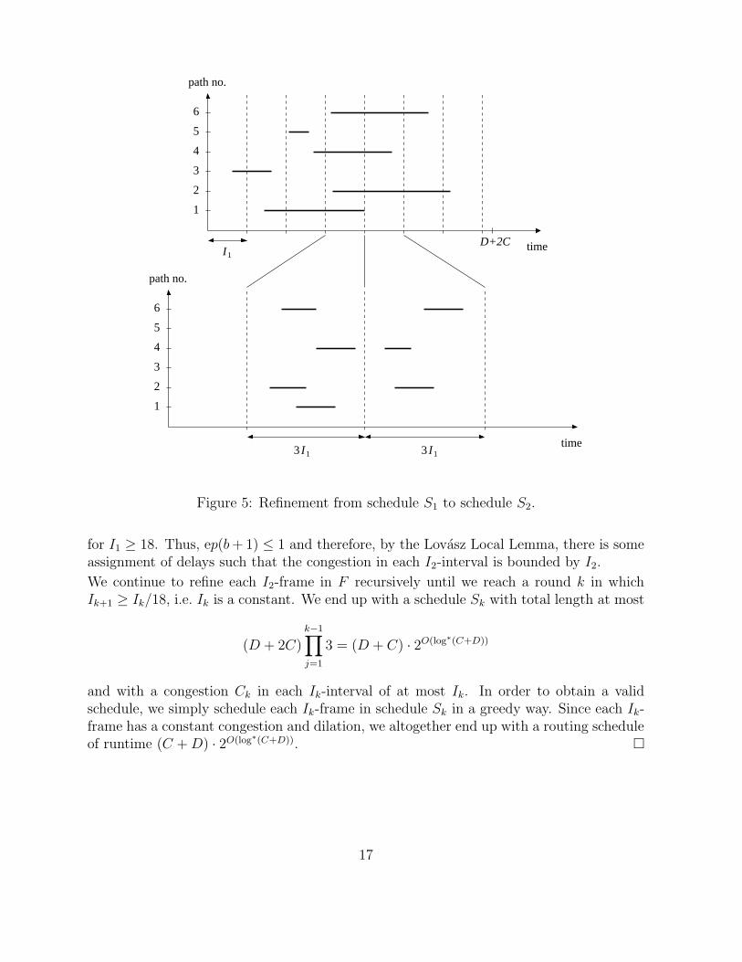
We now break schedule S1 into I1-frames and continue to schedule each frame indepen-dently. So each frame can be viewed as a separate scheduling problem where the origin ofa packet is its location at the beginning of the frame, and its destination is its location atthe end of the frame. Our next refinement step will be to choose, for each frame, a randominitial delay for each packet that visits at least one edge within this frame. In the resultingschedule S2, the frames (enlarged by their delay ranges) are executed one after the otherin a way that a packet that is assigned a delay δ in some frame F waits at its first edgein F for (additional) δ steps, and then moves on without waiting until it traverses its lastedge in F (see Figure 5).

We concentrate in the following on some fixed frame F . Let each packet choose an addi-tional delay out of the range ∆2 = [2I1]. Hence, the length of the resulting schedule for thisframe is at most 3I1. We use the Lovasz Local Lemma to show that if the delays are chosenindependently and uniformly at random, then with nonzero probability the congestion inany I2-interval is at most I2. We again associate a bad event with each edge. The badevent for edge e is that more than I2 packets use e in some I2-interval.

We first bound the dependence of these events. Whether or not a bad event occurs solelydepends on the delays assigned to the packets that pass through the corresponding edge.Since at most I1 packets pass through an edge in any frame and each of these packetspasses through at most I1 other edges, the dependence of the bad events is at most I21 .

Next we bound the probability that a bad event occurs. Consider some fixed edge e andI2-interval J . Let the packets traversing e in F be numbered from 1 to m ≤ I1. For everyi ∈ {1, . . . ,m}, let the binary random variable Xi be one if and only if packet i traversese during J . Let X =

∑mi=1Xi. Since the packets choose their delays uniformly at random

from a range of size 2I1, we get Pr[Xi = 1] ≤ I2/(2I1) for all i ∈ {1, . . . ,m}. Hence,

E [X] =m∑

i=1

E [Xi] ≤ I1 ·I22I1

= I2/2 .

Together with the Chernoff bounds we therefore get with ε = 1 that

Pr [X ≥ I2] = Pr [X ≥ (1 + ε)I2/2] ≤ e−I2/6 ≤ e−3(ln I1+1) = (e · I1)−3 .

Since for each edge there are at most 3I1 many I2-intervals to consider, the probabilitythat a bad event occurs for edge e is bounded by

p ≤ 3I1 · (e · I1)−3 <1

e(I21 + 1)

16

I1

6

5

4

3

2

1

6

5

4

3

2

1

I13 3 I1

path no.

timeD+2C

time

path no.

Figure 5: Refinement from schedule S1 to schedule S2.

for I1 ≥ 18. Thus, ep(b+ 1) ≤ 1 and therefore, by the Lovasz Local Lemma, there is someassignment of delays such that the congestion in each I2-interval is bounded by I2.

We continue to refine each I2-frame in F recursively until we reach a round k in whichIk+1 ≥ Ik/18, i.e. Ik is a constant. We end up with a schedule Sk with total length at most

(D + 2C)k−1∏

j=1

3 = (D + C) · 2O(log∗(C+D))

and with a congestion Ck in each Ik-interval of at most Ik. In order to obtain a validschedule, we simply schedule each Ik-frame in schedule Sk in a greedy way. Since each Ik-frame has a constant congestion and dilation, we altogether end up with a routing scheduleof runtime (C +D) · 2O(log∗(C+D)). ¤

17

5 Online Switching

We saw in the previous section that for every collection of simple paths there is a scheduleto send packets along these paths, one packet per path, so that in at most O(C + D)time steps all packets reach their destinations. The question we want to investigate inthis section is whether a similar runtime can also be achieved for the online case. By“online” we mean that the system has no global knowledge about the routing problem.At the beginning, every processor only knows the packets that start in it (and, maybe,a few global parameters such as the congestion of the path collection). A processor canonly use the information it receives during the routing. Thus, the processors may have dobase their switching decisions on imcomplete information. We will show that neverthelessefficient switching can be done.

5.1 A Switching Protocol for Directed Acyclic Graphs

A directed acyclic graph (or short DAG) is a directed graph that has no directed cycle. Wedemand that any path chosen in a DAG for some routing problem must traverse its edgesin the direction of their orientation, that is, it must be directed. We say that a DAG has adepth of D if the maximum number of edges a directed path can have in it is equal to D.

Suppose that we are given a collection of n paths in a DAG. Along each of these pathsa packet has to be sent. Suppose w.l.o.g. that these packets are numbered from 1 to n.(Any numbering that ensures that no two packets have the same number would suffice.)The random rank protocol sends the packets along their paths in the following way:

At the beginning, every packet i chooses uniformly and independently at random an integerri out of some range [K] (K will be determined later). Let the rank of packet i be definedas rank(i) = ri+

in+1

. These ranks are used in the following way to resolve conflicts amongthe packets.

For every time step and every edge with nonempty buffer, select the packet withminimum rank waiting at it and send it along that edge.

5.2 Analysis of the Switching Protocol

The following time bound has been shown by Leighton, Maggs, Ranade, and Rao.

Theorem 5.1 Suppose we are given an arbitrary path collection P of size n and congestionC in a DAG of depth D. Let K ≥ 8C. Then the random rank protocol needs at most O(C+D + log n) time steps, with high probability, to send all the packets to their destinations.

Proof. Suppose that the runtime of the random rank protocol is equal to T ≥ D + S.We want to show that it is very improbable that S is large. For this we need to find astructure that witnesses a large S. This structure should become more and more unlikely

18

to exist the larger S becomes. The structure we are looking for will be the result of thefollowing backwards argument that is similar to the argument used in Section 1.

Let p1 be some packet that arrived at its destination v0 in step T . We follow p1 backwardsin time until we reach an edge e1 where it was delayed the last time before it reached itsdestination. Let us denote the length (i.e., the number of edges) of the path from thedestination of p1 to e1 (inclusive) by `1 and the packet that delayed p1 by p2. Starting frome1, we now follow p2 backwards in time until we reach an edge e2 where it was delayedby some other packet. We call this packet p3 and denote the length of the path from e1(exclusive) to e2 (inclusive) by `2. Afterwards, we follow p3 backwards in time, and soon, until we arrive at a packet ps+1 that prevented the packet ps at edge es from movingforward. (We will specify later how to choose s in relation to S.) The path from es tov0 recorded by this process in reverse order is called delay path (see Figure 6). It consistsof s contiguous parts of routing paths of length `1, . . . , `s ≥ 0 with

∑si=1 `i ≤ D, since no

directed path can be longer than D. Because of the contention resolution rule it holds thatrank(pi) > rank(pi+1) for all i ∈ {1, . . . , s}. A structure that contains all of these featuresis defined as follows.

se

. . .1

2

s

l 1

1223

p p e p e p

l

v0

Figure 6: The structure of a delay path.

Definition 5.2 (delay sequence) A delay sequence of length s consists of

• s not necessarily different delay edges e1, . . . , es;

• s+ 1 delay packets p1, . . . , ps+1 such that the path of pi traverses ei and ei−1 in thatorder for all i ∈ {2, . . . , s}, the path of ps+1 contains es, and the path of p1 containse1;

• s integers `1, . . . , `s ≥ 0 such that `1 is the number of edges in the path of p1 from e1(inclusive) to its destination, for all i ∈ {2, . . . , s} `i is the number of edges in thepath of pi from ei (inclusive) to ei−1 (exclusive), and

∑si=1 `i ≤ D; and

• s+ 1 integers r1, . . . , rs+1 with 1 ≤ rs+1 ≤ . . . ≤ r1 ≤ K.

A delay sequence is called active if

1. for all i ∈ {1, . . . , s} we have rank(pi+1) < rank(pi) and

2. for all i ∈ {1, . . . , s+ 1} we have brank(pi)c = ri.

19

Now, how does s relate to S? The following lemma gives an answer to this.

Lemma 5.3 If the runtime of the random rank protocol is at least D+ s, then there mustexist an active delay sequence of length s.

Proof. Suppose the random rank protocol needs T ≥ D + s steps. Since for any delaysequence of length s we have

∑si=1 `i ≤ D, it holds that T ≥ ∑s

i=1 `i + s and thereforeT −∑s

i=1 `i − s ≥ 0. In this case, the backwards argument we used above is guaranteedto end with a packet ps+1 that delayed ps at time step T −

∑si=1(`i + 1) + 1 ≥ 1, which

implies that there must be such a packet ps+1. Due to the contention resolution rule, thepackets must fulfill requirement (1) of a delay sequence to be active. Requirement (2) canbe fulfilled by simply setting ri = brank(pi)c. ¤

Thus, if no active delay sequence of length s can be constructed from the given pathcollection and the ranks chosen by the packets, then the runtime of the random rankprotocol can be at most D + s. Hence, all we need to do is to bound the probability thatit is possible to construct a delay sequence of length s. For this we need the following twolemmata.

Lemma 5.4 The number of different delay sequences of length s is at most

n · Cs ·(

D + s

s

)

·(

s+K

s+ 1

)

.

Proof. There are at most(

D+ss

)

possibilities to choose the `i such that∑s

i=1 `i ≤ D.Furthermore, there are n packets from which p1 can be chosen. Since p1 and `1 determinethe edge e1 and the congestion at e1 is at most C, there are at most C possibilities to choosepacket p2. The same holds for the packets p3, . . . , ps+1 at the edges e2, . . . , es. Hence, wealtogether have at most

(

D+ss

)

· n · Cs possibilities to choose the delay packets. Finally,

there are at most(

s+Ks+1

)

ways to select the ri such that 1 ≤ rs+1 ≤ . . . ≤ r1 ≤ K. ¤

Lemma 5.5 No packet can appear twice in an active delay sequence.

Proof. Since the ranks of the packets do not change during the routing, the lemma followsdirectly from requirement (1) for a delay sequence to be active. ¤

Because the packets choose their ranks independently at random, Lemma 5.5 implies thatthe probability that some fixed delay sequence of length s is active (or more precisely, that

20

requirement (2) for a delay sequence to be active is fulfilled) is at most 1/K s+1. Thus,

Pr[The random rank protocol needs at least D + s steps]Lemma 5.3

≤ Pr[there exists an active delay sequence of length s]Lemmata 5.4, 5.5

≤ n · Cs ·(

D + s

s

)

·(

s+K

s+ 1

)

· 1

Ks+1

≤ n · Cs · 2D+s · 2s+K · 1

Ks+1

≤ n · 22s+D+K ·(

C

K

)s

If we set K ≥ 8C and s = K + D + (α + 1) log n, where α > 0 is an arbitrary constant,then

Pr[The random rank protocol needs at least D + s steps]

≤ n · 22s+D+K · 2−3s = n · 2−s+D+K =1

nα

which concludes the proof of Theorem 5.1. ¤

References

[BA91] Marc Baumslag and Fred Annexstein. A unified framework for off-line permu-tation routing in parallel networks. Mathematical Systems Theory, 24:233–251,1991.

[Ben64] V. Benes. Permutation groups, complexes, and rearrangeable multistage con-necting networks. Bell System Technical Journal, 43:1619–1640, 1964.

[Ben65] V. Benes. Mathematical Theory of Connecting Networks and Telephone Traffic.Academic Press, New York, NY, 1965.

[Bol98] Bela Bollobas. Modern Graph Theory. Springer-Verlag, Heidelberg, 1998.

[Fig89] Michael Figge. Permutationsrouting auf hochdimensionalen Gittern. Diplomar-beit, Universit”at Dortmund, 1989.

[HHL88] S. M. Hedetniemi, S. T. Hedetniemi, and A. L. Liestman. A survey of gossipingand broadcasting in communication networks. Networks, 18:319–349, 1988.

[LMR88] Tom Leighton, Bruce M. Maggs, and Satish B. Rao. Universal packet routingalgorithms. In Proceedings of the 29th IEEE Symposium on Foundations ofComputer Science (FOCS), pages 256–271, 1988.

21

[LMRR94] Tom Leighton, Bruce M. Maggs, Abhiram G. Ranade, and Satish B. Rao.Randomized routing and sorting on fixed connection networks. Journal ofAlgorithms, 17:157–205, 1994.

[LPV81] Gavriela F. Lev, Nicholas Pippenger, and Leslie G. Valiant. A fast parallel algo-rithm for routing in permutation networks. IEEE Transactions on Computers,30:93–100, 1981.

[NS82] David Nassimi and Sartaj Sahni. Parallel algorithms to set up the Benes per-mutation network. IEEE Transactions on Computers, 31:148–154, 1982.

[Par80] D. Parker. Notes on shuffle/exchange-type switching networks. IEEE Trans-actions on Computers, C-29:213–222, 1980.

[Voc01] B. Vocking. Almost optimal permutation routing on hypercubes. In Proceedingsof the 33rd ACM Symposium on Theory of Computing (STOC), pages 530–539,2001.

[Wak68] A. Waksman. A permuting network. Journal of the ACM, 15:159–163, 1968.

22