Embed Size (px)
Citation preview
ADMLC/2021/4
This study was funded by the UK Atmospheric Dispersion Modelling Liaison Committee.
The views expressed in this report are those of the authors, and do not necessarily
represent the views of ADMLC or of any of the organisations represented on it
A Review of Approaches to Dispersion Modelling of Odour Emissions and Intercomparison of Models and Odour Nuisance Assessment Criteria
C.S. Price1, J. Stocker1, K. Johnson1, R. Patel1, S. Strickland1
J. Doktarova2, J Rubinis2
1 Cambridge Environmental Research Consultants Ltd
(CERC)
2 SIA Estonian, Latvian and Lithuanian Environment (ELLE)
ABSTRACT
Dispersion modelling plays an important role in the assessment of potential odour
annoyance. This review covers the technical approaches used for a range of
dispersion modelling methodologies for the assessment of odour nuisance.
Firstly, a review is presented of the different approaches used to define odour
criteria in different countries, and the range of dispersion modelling methods that
result from them. A literature review is included, summarising different models
used for odour dispersion modelling, and existing validation studies relating to
odour dispersion modelling, with the main features and findings of selected studies
outlined.
A model intercomparison study is presented, covering four datasets including data
from: field odour inspections; field and wind tunnel tracer experiments; and
continuous odour monitoring. Results from three different dispersion models are
included: ADMS, AERMOD and AUSTAL2000. Different criteria are compared, with
a particular focus on the 98th percentile of hourly average concentrations and the
approach involving concentration fluctuations and odour hours.
Finally, the efficacy of different modelling approaches and techniques is discussed,
including validation challenges and methods of estimating concentration
fluctuations. Key factors reviewed include dose-response, peak-to-mean ratios,
statistical methods and fluctuation models.

CONTRACT REPORT FOR ADMLC iii
EXECUTIVE SUMMARY
Dispersion modelling plays an important role in the assessment of odour, not just
because of its predictive value in assessing proposed developments, but because
of the inherent difficulty of quantifying odour intensities in ambient air.
The report begins with an introduction to the key concepts involved in the complex
challenges of odour assessment, such as the importance of transient exposure and
peak concentrations, quantifying or defining the offensiveness of different odour
mixtures, and accounting for different levels of receptor sensitivity.
The first odour regulations and odour criteria in Europe were developed in the
1970s, and questions of the applicability of different criteria and methodologies
still remain the subject of much attention and debate. Here, a review of the
different types and approaches of international odour criteria is presented, along
with the different dispersion modelling methods that result from them. A range of
countries and jurisdictions are selected to demonstrate the different types of
criteria, and highlight any aspects particularly relating to dispersion modelling.
A literature review of validation studies of dispersion models is presented. This
summarises different models used for odour dispersion modelling and validation
studies relating to odour dispersion modelling, with the main features and findings
of selected studies outlined. In general, it was found that there are relatively few
relevant robust validation studies for odour annoyance, adverse impact and/or
nuisance.
The next section of the report comprises a model intercomparison study, using
three models. Four datasets are employed, including data from field experiments,
wind tunnel experiments, and monitoring studies, and techniques including tracer
release, human panel field inspections and electronic nose measurements. The
four datasets examined are as follows:
• OROD
• Field experiments at a pig farm with SF6 tracer and odour
measurements
• 10-minute and some shorter (10-second) measurements
• CEDVAL
• High frequency wind tunnel measurements
• Set-up based on the OROD dataset
• Riga Port
• Continuous long-term electronic nose odour measurements at three
locations
• 1-minute averages
• Styria pig farm
• Field experiment with odour field inspection measurements

iv CONTRACT REPORT FOR ADMLC
Three different models, ADMS, AERMOD and AUSTAL2000, are included in the
intercomparison study. ADMS and AERMOD are advanced Gaussian plume models,
and AUSTAL2000 is a Lagrangian particle model. Different criteria are compared,
with a particular focus on the 98th percentile of annual hourly average
concentrations and the approach involving concentration fluctuations and odour
hours. The fluctuations module of ADMS is used to assess short-term
concentrations and odour hours, and peak-to-mean factors are explored with all
models. The findings are compared with existing studies carried out for the same
datasets.
The efficacy of the two main modelling approaches and techniques is discussed:
a) the 98th percentile of hourly average concentrations approach and b) the sub-
hourly average approach.
For the 98th percentile hourly average approach, the development of the criteria,
via dose-response studies, is discussed. An analysis of the relevant validation
studies, and the challenges involved in validating this type of criteria, are outlined.
An analysis is presented of the factors that determine how well, and in what
circumstances, the criteria can predict annoyance or adverse odour impacts. An
outline of possible improvements to the use of the criteria is suggested; this
involves the use of different percentile values for different applications.
For the sub-hourly approach, an investigation into the main factors that determine
peak-to-mean ratios of concentrations is presented. These depend both on the
within-plume fluctuations due to turbulent mixing, and crosswind advection of the
plume by turbulence and wind meandering. Important factors include the
downwind and crosswind location of receptors, the source type and height and the
atmospheric stability. Methods commonly used for estimating short-term
concentrations in dispersion modelling are reviewed, including the application of a
single, fixed peak-to-mean factor, the use of variable peak-to-mean factors based
on simple functions, and statistical predictions of fluctuations by means of
probability distribution functions, derived according to the modelled ensemble
mean concentration and the characteristics of the ambient turbulence.
A key finding of the research is a recognition of the need for more datasets,
through generation of new data and/or collation, organisation and dissemination
of existing data. These include datasets with which the efficacy of odour criteria
can be directly tested, particularly the 98th percentile of hourly average criteria,
and datasets with which dispersion modelling results can be validated. There is
also a clear requirement for more data on odour emission rates and emission
factors for various sectors, sources and types of odour, under varying conditions.
Improvements in accuracy and more widespread use of technology such as
electronic noses show promising potential in helping to create useful datasets. A
transition from discrete odour measurements to a more monitoring-based
approach could provide a valuable opportunity to improve the understanding of
spatial and temporal trends of odour sources that would in turn inform dispersion
modelling, much in the way that the monitoring of other air pollutants has done.
CONTRACT REPORT FOR ADMLC v
CONTENTS
1 Introduction 1
2 Key concepts in odour criteria and assessment 2 2.1 Odour nuisance and FIDOL 2 2.2 Odour criteria: an overview 2 2.3 Peak and hourly average concentrations 3 2.4 Modelling peak and hourly average concentrations 4 2.5 Odour hours 5
3 Assessment criteria and methodology in different countries 7 3.1 Australia 7 3.2 Austria 12 3.3 Czech Republic 12 3.4 Estonia 12 3.5 Germany 13 3.6 Ireland 14 3.7 Italy 14 3.8 Latvia 15 3.9 Lithuania 15 3.10 The Netherlands 16 3.11 New Zealand 16 3.12 United Kingdom 16 3.13 Summary of criteria in the selected countries 18
4 Models used for odour assessment 21 4.1 Gaussian Plume models 21 4.2 Lagrangian models 21 4.3 Examples of models commonly used for odour dispersion
modelling 21
5 Validation studies 24 5.1 Measurement methods used in odour model validation studies 24 5.2 Selected validation studies 25
5.2.1 Conclusions 31
6 Model Intercomparison 33 6.1 Overview of models and datasets used 33 6.2 OROD dataset 34
6.2.1 General experimental setup 34 6.2.2 Data provided 37 6.2.3 Model runs 37
6.3 CEDVAL dataset 42 6.3.1 General experimental setup 42 6.3.2 Data provided 42 6.3.3 Model runs 42
6.4 Riga Port dataset 49 6.4.1 Assessment area 49 6.4.2 Monitoring data 51 6.4.3 Modelled sources 54 6.4.4 Meteorological data 56
vi CONTRACT REPORT FOR ADMLC
6.4.5 ADMS model runs 57 6.4.6 AUSTAL2000 runs 66
6.5 Styria pig farm dataset 69 6.5.1 Experimental setup and dataset 69 6.5.2 Model runs 71
6.6 Summary 76
7 Efficacy of the different approaches in odour dispersion
modelling 77 7.1 Percentile of hourly averages approaches 77
7.1.1 The origin of the criteria 77 7.1.2 Challenges for validation 78 7.1.3 Trends and reasons for poor prediction in validation
studies 79 7.1.4 Possible modifications using variable percentile values 81
7.2 Sub-hourly average approaches 83 7.2.1 Real world – what affects peak concentrations and
fluctuations? 83 7.2.2 Peak-to-mean ratio modelling approaches 84 7.2.3 Statistical approaches 86
7.3 Universal challenges in odour dispersion modelling 90
8 DISCUSSION 92
Acknowledgements 93
References 94
Introduction
CONTRACT REPORT FOR ADMLC 1
1 INTRODUCTION
The first odour regulations and odour impact criteria were introduced in Europe in the
1970s and questions of the applicability of different criteria and methodologies still remain
the subject of much attention and debate. There are several publications that give an
account of the history of the development of odour criteria. The Institute of Air Quality
Management (IAQM) Odour Guidance document (Bull et al, 2014), for example, gives a
very detailed account of the evolution of odour regulation in the UK and Europe.
Internationally, there is a broad variety of odour nuisance criteria and approaches. Criteria
from selected countries and regions are described in this review, to give an overview of
the different approaches.
Dispersion modelling has played an important role in the assessment of odour, not just
because its predictive capacity is helpful and important in assessing proposed
developments, but also because of the inherent difficulty of quantifying odour intensities
in ambient air. Just as there are several approaches to odour impact and nuisance criteria,
there are also several approaches to dispersion modelling. The main types of models and
modelling methodologies are examined in this review.
2 CONTRACT REPORT FOR ADMLC
2 KEY CONCEPTS IN ODOUR CRITERIA AND ASSESSMENT
2.1 Odour nuisance and FIDOL
A useful starting point for describing the important concepts in odour nuisance assessment
is the FIDOL framework concept:
• Frequency
• Intensity
• Duration
• Offensiveness
• Location
The Frequency relates to how often an individual is exposed to an odour over relatively
short timescales, and to the frequency of detection. Individuals can become habituated to
a consistent stimulus of odour, becoming unable to detect this odour after a certain period;
this is an adaptation known as olfactory fatigue. If, however, the exposure to odour has
an on/off/on pattern, this adaptation process is disrupted, and the odour can be repeatedly
perceived, and hence cause annoyance and ultimately may cause or constitute a nuisance.
The Intensity is essentially the concentration or strength of the odour. Technically, it is
the perception of the strength of the odour, an important distinction, since the relationship
between a stimulus (smell, noise, brightness, etc.) and its perceived strength is not
necessarily linear. The intensity of an odour is widely understood to be a logarithmic
function of its concentration. The human response to odour is a complex topic and is not
covered in this review.
The third FIDOL factor is the overall Duration of the exposure. This covers the relatively
long temporal patterns of the exposure, such as hourly, daily and seasonal patterns, or
the length of a particular odour ‘episode’.
The Offensiveness (sometimes called the Odour unpleasantness) refers to the character
of the odour at a given intensity and ability to induce a reaction of pleasure or displeasure.
This can be related to, or expressed as, the ‘hedonic tone’ of the odour, and can be
quantified as a ‘hedonic’ score of the odour’s ability to induce pleasure or displeasure in
the individual.
The Location refers to the nature of the area surrounding the odour source and the
sensitivity of nearby receptors. This is often related to the land use, such as whether it is
predominantly residential or industrial, or urban or rural in character.
2.2 Odour criteria: an overview
Internationally, there is a diverse range of odour criteria for dispersion modelling, but all
basically comprise three constituent parts: a percentile value; an averaging time; and a
threshold value.
Key concepts in odour criteria and assessment
CONTRACT REPORT FOR ADMLC 3
The percentile value is a measure of the probability of exceedence of a threshold within a
defined period, or the value that is exceeded for a specific percentage of the time. The
averaging time relates to the exposure duration; its value, relative to the duration of a
human breath and to the response time of the human nose, is an important concept. The
threshold value is the odour concentration that is considered to represent the onset of
odour annoyance. This is a value with which the results of dispersion modelling can be
compared.
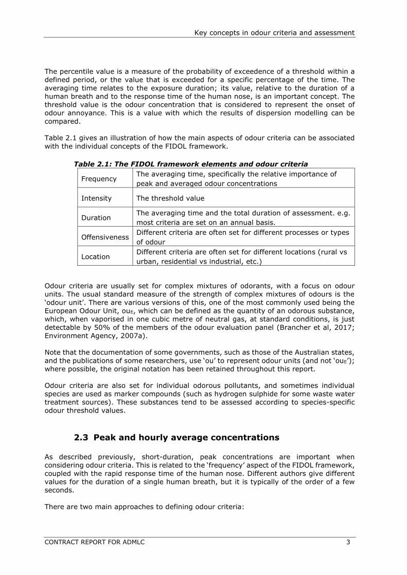
Table 2.1 gives an illustration of how the main aspects of odour criteria can be associated
with the individual concepts of the FIDOL framework.
Table 2.1: The FIDOL framework elements and odour criteria
Frequency The averaging time, specifically the relative importance of
peak and averaged odour concentrations
Intensity The threshold value
Duration The averaging time and the total duration of assessment. e.g.
most criteria are set on an annual basis.
Offensiveness Different criteria are often set for different processes or types
of odour
Location Different criteria are often set for different locations (rural vs
urban, residential vs industrial, etc.)
Odour criteria are usually set for complex mixtures of odorants, with a focus on odour
units. The usual standard measure of the strength of complex mixtures of odours is the
‘odour unit’. There are various versions of this, one of the most commonly used being the
European Odour Unit, ouE, which can be defined as the quantity of an odorous substance,
which, when vaporised in one cubic metre of neutral gas, at standard conditions, is just
detectable by 50% of the members of the odour evaluation panel (Brancher et al, 2017;
Environment Agency, 2007a).
Note that the documentation of some governments, such as those of the Australian states,
and the publications of some researchers, use ‘ou’ to represent odour units (and not ‘ouE’);
where possible, the original notation has been retained throughout this report.
Odour criteria are also set for individual odorous pollutants, and sometimes individual
species are used as marker compounds (such as hydrogen sulphide for some waste water
treatment sources). These substances tend to be assessed according to species-specific
odour threshold values.
2.3 Peak and hourly average concentrations
As described previously, short-duration, peak concentrations are important when
considering odour criteria. This is related to the ‘frequency’ aspect of the FIDOL framework,
coupled with the rapid response time of the human nose. Different authors give different
values for the duration of a single human breath, but it is typically of the order of a few
seconds.
There are two main approaches to defining odour criteria:

4 CONTRACT REPORT FOR ADMLC
a) Those that are based on an hourly average concentration, and
b) Those that incorporate some consideration of peak concentrations.
Approach (a) involves the application of some high percentile value (such as the 98th
percentile) to the hourly averaged concentrations.
Approach (b) requires the calculation of concentrations over an averaging/sampling time
that is much less than an hour (sub-hourly concentrations).
There are significant advantages/disadvantages to each approach. For approach (a), based
on hourly average concentrations, a key advantage is that hourly-averaged inputs such as
meteorological data are very commonly used in dispersion modelling, and hourly-averaged
output is standard for regulatory modelling. The approach is also based on relatively simple
concepts and straightforward methodologies. The approach is well-established, having
been widely used in many countries, in many different practical situations, and has been
the subject of much scrutiny such as during legal disputes and planning appeal hearings.
The disadvantages are that this approach does not directly (at the modelling stage) take
into account the brief periods of high concentrations that can be sampled and detected by
the human olfactory system, and be experienced by the receptor as a variable on/off signal,
potentially overcoming olfactory fatigue and causing nuisance.
For approach (b), the main advantage is that it does take into account these peak
concentrations, and the frequency of the exposure, and some evidence suggests that this
can be a better indicator of odour annoyance than the alternative approach. Another
advantage in general is that it can be assessed using both field measurements and
dispersion modelling, whereas approach (a) can only be assessed by dispersion modelling
(Oettl et al, 2018). The main disadvantage of this approach is that modelled peak
concentrations have greater uncertainty, since the stochastic nature of the atmospheric
phenomena - the turbulent processes and wind meandering - that determine the peaks,
are not deterministic, but need to be described by probability distributions or simplified
models. In addition, the precise relationship between odour frequency and odour nuisance
is not fully understood (e.g. Griffiths et al, 2014).
2.4 Modelling peak and hourly average concentrations
Fluctuations in concentrations are caused by changes in the mean wind direction and
advection and mixing by atmospheric turbulence. Although turbulence exists on a
continuum of spatial and temporal scales, it can be useful to conceptually distinguish
between different sizes of eddy in relation to the size of a plume. Where eddies are large
compared to the width of a plume (e.g. close to the source), they generally act to transport
the plume as a whole (plume meander). Eddies that are smaller than the plume dimensions
mix ambient air into and within the plume, mixing and spreading the plume on a finer
spatial scale.
Smaller-scale turbulent processes are more important for shorter averaging times, and
these processes are inherently challenging to model explicitly. There are various ways of
approaching regulatory odour dispersion modelling, to try to take into account the
fluctuations in concentrations, due to turbulent effects, on a sub-hour scale; these depend
on the general type of odour criterion that is being assessed, and the level of detail of the
model.
One method of dispersion modelling is used to address the hourly-average criteria
(approach (a) listed above). It is based solely on hourly average concentrations, and the
Key concepts in odour criteria and assessment
CONTRACT REPORT FOR ADMLC 5
dispersion model outputs a concentration that corresponds to a specific percentile of the
hourly average.
The remaining methods for dispersion modelling are used to address the requirement for
a sub-hourly concentration (approach (b) above).
One such approach involves dispersion calculations to calculate an hourly averaged
concentration, followed by a simple factor to convert the hourly averaged concentrations
to sub-hour peak concentrations. This second step may be carried out by the software, or
by the model user. This approach is often called the ‘peak-to-mean’ approach, as it uses
the ratio of the peak concentration to the mean concentration as a factor. Post-dispersion
step peak-to-mean ratios are sometimes used in regulatory modelling to convert hourly
averaged concentrations to a peak concentration.
Schauberger et al (2012) discuss how “An open question is the definition of the peak value,
Cp” They list four different commonly used definitions of ‘peak’ in peak-to-mean ratios
(where the mean concentration, Cm, represents an hour and the peak concentration a
shorter period):
1. Cp = Cm + where is the standard deviation
2. Cp is the 90th percentile of sub-hourly averaged concentrations
3. Cp is the 98th or 99th percentile
4. Cp is the maximum (100th percentile)
A commonly applied method, used by models such as AUSTAL2000, is to use a single peak-
to-mean conversion factor (e.g. Schauberger et al, 2012). In other cases, a range of peak-
to-mean ratio values are used to account for the fact that this ratio varies both spatially
and temporally (e.g. Piringer et al, 2016) as the plume mixes with ambient air and is
advected by it. Factors that affect the mixing, and hence the peak-to-mean values, include
the distance from the source, atmospheric stability, the presence of buildings and other
obstacles and the source type. For the source type, an important distinction is whether the
release is controlled (e.g. emitted via a stack or vent), or in the form of more uncontrolled
leaks (‘fugitive’ emissions).
Other modelling methods use statistical approaches that estimate the probability of
exceedence by assuming a distribution function, depending, for example, on the modelled
mean plume properties and turbulence characteristics of the ambient air (e.g. Davies et
al, 1998).
Model algorithms have been developed that use other, more sophisticated methods of
calculating peak sub-hourly average concentrations, but these have not historically been
routinely used to model odour in a regulatory context.
These factors are discussed in more detail in later sections of this report.
2.5 Odour hours
Once peak concentrations have been determined, these then need to be translated into a
measure of annoyance. Some sub-hour averaging time criteria are based on a
straightforward percentile statistic, but others are based on a concept called the ‘odour
hour’.
6 CONTRACT REPORT FOR ADMLC
The odour hour approach is used primarily in Germany and Austria. An odour hour is one
in which there is a recognisable odour detected for a specified proportion of the hour. Note
that this does not necessarily have to correspond to continuous periods of time. In German
and Austrian regulations, odour hours are defined as having recognisable odour for at least
10% of the time (6 minutes). Therefore, the definition of the peak sub-hourly concentration
is the 90th percentile.
The odour assessment is then continued by summing the number of odour hours over the
year, and this value, expressed as a percentage of the total number of hours, is then
compared with threshold values.
Note that the absolute magnitude of an odour concentration is not a consideration for the
odour hour approach, beyond a simple yes/no condition for exceedence of the odour
threshold. In addition, the application of this approach means that a large number of short
odour episodes can be assigned more importance than a smaller number of long episodes.

Assessment criteria and methodology in different countries
CONTRACT REPORT FOR ADMLC 7
3 ASSESSMENT CRITERIA AND METHODOLOGY IN DIFFERENT COUNTRIES
Reviews by Brancher et al (2017) and Bokowa et al (2021) have comprehensively collated
and described the odour criteria in a wide variety of countries and regions. The current
review does not repeat all of this information in detail, and the reader is referred instead
to the aforementioned reviews.
The main criteria for selected countries and regions are outlined in this section, together
with any key information relating to dispersion modelling. The countries and regions were
selected to demonstrate the different type of criteria, to highlight any aspects particularly
relating to different dispersion modelling approaches, and to identify any recent changes
to the criteria. In addition, the criteria of several countries are considered that were not
included in the aforementioned reviews.
3.1 Australia
The odour criteria and dispersion modelling methodologies in Australia are of particular
note because the constituent states have widely varying odour impact criteria and
assessment methodologies, and there have recently been interesting changes in the
regulations for some of the states. The criteria for each of the states are outlined below.
New South Wales
Until recently, two odour assessment guidance documents, the overall ‘Technical
Framework’ (New South Wales, 2006a) and the accompanying ‘Technical Notes’ (New
South Wales, 2006b), provided the odour assessment methodology guidance for New
South Wales.
Updated New South Wales general air pollutant assessment guidance (New South Wales
EPA, 2017) now outlines the odour assessment methodology and criteria, for both the total
odour (complex mixtures of odorants) and individual odorous species. It is this guidance
that is referred to here.
The 2017 guidance describes two levels of impact assessment:
• Level 1 – screening-level dispersion modelling techniques using worst-case input data
• Level 2 – refined dispersion modelling techniques using site-specific input data.
For complex mixtures of odour, the assessment criteria are defined in terms of peak
concentrations over a ‘nose response time’ averaging time (taken to be 1 second), and are
population density-specific. The criteria are based on the 100th percentile of 1-second
averaged concentrations for Level 1 assessments, and the 99th percentile of 1-second
averages for Level 2 assessments. The thresholds for each population density band are
given in Table 3.1.

8 CONTRACT REPORT FOR ADMLC
Table 3.1: Thresholds for complex odour mixtures
Population of affected community Threshold (ou)
Urban (>~2000) and/or schools and hospitals 2
500 3
125 4
30 5
10 6
Single rural residence (<2) 7
For individual odorants, threshold values are substance-specific. The assessment criteria
are based on hourly averages, at the 100th percentile for Level 1 assessments, and the
99.9th percentile for Level 2 assessments. It is interesting to note that there is a single
exception to this, hydrogen sulphide, which is to be treated with the same averaging time
and percentiles as the complex odour mixtures.
Regarding dispersion models (for general, not only odour, assessments), the guidance
states that AUSPLUME (version 6.0 or later) is “the approved dispersion model for use in
most simple, near-field applications in NSW, where coastal effects and complex terrain are
of no concern.” The situations for which it is not approved are those that involve: complex
terrain and non-steady state conditions; buoyant line sources; coastal effects; a high
frequency of calm, stable night-time conditions; a high frequency of calm conditions and
inversion break-up fumigation conditions.
It then explains that there may be other situations in which AUSPLUME may not be
appropriate, and suggests that CALPUFF (version 5.7 or later) or TAPM (version 2.0 or
later) (CSIRO, 2008) may be appropriate for these conditions. It also states that other
dispersion models may be used, following consultation with the EPA, and justification that
the model is scientifically sound for its proposed application.
For dispersion modelling of peak concentrations for odour assessments, the guidance
provides peak-to-mean ratios for estimating the ‘extreme’ (1-second average) peak
concentrations from hourly averages, for different source types, stabilities and distances
from the source. These are reproduced in Table 3.2.
Table 3.2 Peak-to-mean ratios for estimating 1-s averages
Source type Pasquill–Gifford
stability class
Peak-to-mean ratio
Near-field Far-field
Area A,B,C,D 2.5 2.3
E,F 2.3 1.9
Line A-F 6 6
Surface wake-free point A,B,C 12 4
D,E,F 25 7
Tall wake-free point A,B,C 17 3
D,E,F 35 6
Wake-affected point A-F 2.3 2.3
Volume A-F 2.3 2.3
Assessment criteria and methodology in different countries
CONTRACT REPORT FOR ADMLC 9
Queensland
Guidance published in 2013 for odour impact assessment (Queensland, 2013) provides
substantial and prescriptive detail on the dispersion modelling methodology for odour and
the criteria to be used.
The guidance distinguishes between total odour, odour indicator species and single odorous
species. It also has one set of criteria for ground level sources and ‘wake-free’ stacks, and
another for ‘wake-affected’ stacks; the definition of a wake-free stack being one that has
a height that is 2.5 times greater than the height of any nearby building.
For total odour, for proposed new facilities, the guideline values are a 99.5th percentile of
1-hour average concentrations, with a limit of 0.5 ou for wake-free stacks, and 2.5 ou for
ground-level or wake-affected stacks.
They explain that they consider the general understanding of peak-to-mean factors to be
insufficient to justify setting criteria based on averaging times of less than an hour. Instead
the above hourly average criteria were determined, based on a threshold of 5 ou with a
peak-to-mean ratio of 10:1 for wake-free stacks and 2:1 for ground-level sources or wake-
affected stacks.
For individual odorous pollutants, various criteria from other Australian states are
referenced. The guidance acknowledges the need for caution in converting the hourly
averages to three-minute averages.
The guidance does not recommend the use of any specific dispersion model; it states that
the appropriate model should be selected based on the requirements of each particular
case, “in order to allow scientific and technical advances to be introduced without
regulatory delays”. The use of AUSPLUME is accepted “for most near-field assessments of
odour sources located in relatively flat terrain and as an initial screening model”. CALPUFF,
AERMOD, ADMS and TAPM are listed as advanced models that could be used as an
alternative.
The guidance specifies that time-variation of emissions should be included in the modelling,
and that where facilities do not operate continuously, the 99.5th percentile must be applied
to the actual hours of operation. It notes the uncertainties involved in modelling variable
short-term peak emissions such as turning of compost windrows. For existing facilities, the
2013 guidance allows alternative assessment methodologies.
The guidance states that all relevant sources of odour, both on the operator’s site and on
nearby sites, should be included in the dispersion modelling, and stresses the importance
of the inclusion of fugitive emissions.
There is also specific odour guidance for the poultry industry with more stringent odour
criteria (Queensland, 2011; Queensland, 2016). The 99th percentile of hourly averages is
specified, but here the thresholds are 2.5 ou for a sensitive land use in a rural zone and
1ou for the boundary of a non-rural zone.
South Australia
The odour assessment guidance for South Australia is incorporated within its ‘Ambient air
quality assessment’ guidance, published in 2016 (South Australia, 2016a). This supersedes
the previous odour guidance published in 2007.
This refers to odorous mixture criteria in Schedule 3 of the Environment Protection (Air
Quality) Policy 2016 (South Australia, 2016b), which are dependent on population density
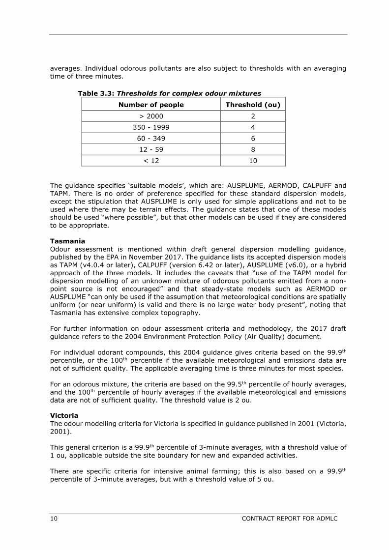
as shown in Table 3.3. Note that the thresholds refer to the 99th percentile of three-minute
10 CONTRACT REPORT FOR ADMLC
averages. Individual odorous pollutants are also subject to thresholds with an averaging
time of three minutes.
Table 3.3: Thresholds for complex odour mixtures
Number of people Threshold (ou)
> 2000 2
350 - 1999 4
60 - 349 6
12 - 59 8
< 12 10
The guidance specifies ‘suitable models’, which are: AUSPLUME, AERMOD, CALPUFF and
TAPM. There is no order of preference specified for these standard dispersion models,
except the stipulation that AUSPLUME is only used for simple applications and not to be
used where there may be terrain effects. The guidance states that one of these models
should be used “where possible”, but that other models can be used if they are considered
to be appropriate.
Tasmania
Odour assessment is mentioned within draft general dispersion modelling guidance,
published by the EPA in November 2017. The guidance lists its accepted dispersion models
as TAPM (v4.0.4 or later), CALPUFF (version 6.42 or later), AUSPLUME (v6.0), or a hybrid
approach of the three models. It includes the caveats that “use of the TAPM model for
dispersion modelling of an unknown mixture of odorous pollutants emitted from a non-
point source is not encouraged” and that steady-state models such as AERMOD or
AUSPLUME “can only be used if the assumption that meteorological conditions are spatially
uniform (or near uniform) is valid and there is no large water body present”, noting that
Tasmania has extensive complex topography.
For further information on odour assessment criteria and methodology, the 2017 draft
guidance refers to the 2004 Environment Protection Policy (Air Quality) document.
For individual odorant compounds, this 2004 guidance gives criteria based on the 99.9th
percentile, or the 100th percentile if the available meteorological and emissions data are
not of sufficient quality. The applicable averaging time is three minutes for most species.
For an odorous mixture, the criteria are based on the 99.5th percentile of hourly averages,
and the 100th percentile of hourly averages if the available meteorological and emissions
data are not of sufficient quality. The threshold value is 2 ou.
Victoria
The odour modelling criteria for Victoria is specified in guidance published in 2001 (Victoria,
2001).
This general criterion is a 99.9th percentile of 3-minute averages, with a threshold value of
1 ou, applicable outside the site boundary for new and expanded activities.
There are specific criteria for intensive animal farming; this is also based on a 99.9th
percentile of 3-minute averages, but with a threshold value of 5 ou.
Assessment criteria and methodology in different countries
CONTRACT REPORT FOR ADMLC 11
A major change in regulatory dispersion modelling guidance occurred in 2014, when
AUSPLUME was replaced by AERMOD as the air pollution dispersion regulatory model in
Victoria.
Victoria EPA published guidance regarding the use of AERMOD (Victoria, 2013), which
includes a methodology for estimating 3-minute average concentrations from hourly
averages. This is a post-processing step, where the following formula should be applied:
c(t) = c(t0) (t0/t)0.2
where c is the concentration, t is the averaging time (3 minutes), and t0 is the model output
averaging time (60 minutes). That is, a fixed peak-to-mean factor of 1.82 is applied.
This guidance also explains that alternative dispersion models, such as CALPUFF and TAPM,
may be used in some cases, such as those where the dispersion is affected by coastal
effects or complex terrain. This requires approval from the EPA, and a demonstration that
the model is appropriate for the circumstances. EPA guidance from 2017 expresses the
opinion that “currently CALPUFF is the most appropriate model for modelling air dispersion
from broiler farms and recommends its use…”, and that this constitutes the required
written approval for its application in such cases (Victoria, 2017).
Western Australia
Western Australia published a Guideline in June, 2019 (Western Australia, 2019),
specifying an odour modelling methodology that is a distinct departure from previous
guidance. It is based on the concept of ‘comparative modelling’, which is “the comparison
of two or more modelling scenarios (e.g. using different pollution control equipment)
without specific reference to air emission criteria.” This involves calculating the relative
impact of different modelling scenarios, as opposed to generating absolute total odour
concentrations. Examples of different modelling scenarios are changes in emissions due to
mitigation techniques, or changes in number or configuration of sources.
The draft guidance states that ‘criterion modelling’ is not accepted for odour impact
assessment purposes because of large uncertainties associated with this. This rejection of
criteria-based dispersion modelling is repeatedly and strongly stated throughout the
guidance.
The recommendation is that the 99.5th percentile of hourly averaged concentrations are
reported for the relative dispersion modelling assessments, with the explanation that
“concentrations of this percentile are less prone to issues relating to intermittent emissions
than lower percentiles and are less sensitive to the statistical robustness issues of higher
percentiles.”
The guidance states that limit values from the European Standard EN 16841 1:2016 (CEN,
2016a) or German Guidelines (such as 10% ‘odour hours’) “have not been demonstrated
to be applicable to Western Australian conditions” and stipulates that these values must
not be used for odour assessments.
Regarding dispersion models, the guidance states that the selection of models is at the
discretion of the applicant, providing that the model is appropriate for use. It goes on to
state that “simpler models such as steady-state Gaussian models may provide acceptable
results for some relative odour modelling scenarios”.
Note that previous odour assessment guidance for Western Australia stated criteria based
on the 99.5th and 99.9th percentiles of 3-minute averages.
12 CONTRACT REPORT FOR ADMLC
3.2 Austria
Austria uses the ‘odour hour’ approach to odour assessment, as described in Section 2.5,
where an odour hour is said to have occurred if there has been a recognisable odour for at
least 10% of the time (6 minutes) in any hour.
Austrian air quality regulations include limit values (which have a legal basis) and target
values (which have no legal basis, and act as guidelines only). For odour, there are only
target values, so there are currently no legally binding quantitative criteria for the control
of odour. This means that there are no national criteria to define the number of odour
hours permitted per year, and different regions of Austria have assigned their own values
for this.
Some regions use a limit of 8% odour hours for ‘weak’ odours and 3% for ‘strong’ odours.
If the number of permitted odour hours is expressed as a percentile, then this equates to
92 and 97 percentiles for weak and strong odours, respectively. A problem with this
approach is that the definition of ‘weak’ and ‘strong’ odours is open to interpretation. Some
regions use the odour hour limits from the German regulations, and the remainder use a
mixture of the German regulations and the 8% and 3% values.
Note that it is only in Austria that dynamically varying peak-to-mean ratios are applied in
a regulatory context. No particular dispersion model is stipulated, but models that have
been used to calculate the short-term concentrations include AODM, LASAT (Piringer et al,
2016) and GRAL (Oettl et al, 2018a).
There has been significant attention given to the Austrian odour guidelines in recent years
(e.g. Oettl et al, 2018b).
3.3 Czech Republic
In the Czech Republic, odour is managed at the regional level, and in relatively general
and voluntary terms, with no legally defined maximum exposure levels (Dousa, 2019). Act
No 201/2012 Coll. on Air Protection states that the Ministry of the Environment sets general
and specific emission limit values, and details the method used to set specific emission
limit values for odour nuisances. Decree of the Ministry of Environment No 415/2012 Coll.,
on the permissible level of air pollution and its determination, states that the specific
emission limit value for the pollutant or group of pollutants with potential to cause an odour
nuisance is determined by the following procedure:
• the amount of odorous pollutant or group of odorous pollutants is determined
• appropriate primary and secondary measures are identified to reduce the odour nuisance with
regard to technology and its effectiveness
• following the determined starting amount of odorous pollutants, the selected measures and
their effectiveness shall determine the output quantity of odorous pollutants in the waste gas
3.4 Estonia
The Estonian Atmospheric Air Protection Act introduces the term ‘unpleasant or irritant
odour’. The act also states that the combined impacts of several odour-generating
Assessment criteria and methodology in different countries
CONTRACT REPORT FOR ADMLC 13
installations has to be evaluated, sets the requirements for development and minimum
requirements for a plan for reducing the presence of odoriferous substances, as well as the
procedure for approval and review of such a plan.
The Estonian Regulation for odour assessment is largely based on the German approach
to odour management, VDI 3788 Part 1 (Germany, 2000) and covers the following key
issues:
• approved standards for odour assessment
• procedure for assessment of odour
• odour target values
According to this regulation, the degree of odour disturbance not to be exceeded is
expressed as a percentage of annual odour hours throughout a year, and depends on the
type of odour measurement applied:
1. If odour analysis is carried out according to the standard EVS 886-1:2005 ‘Environmental
Meteorology Dispersion of odorants in the atmosphere – Fundamentals’, then less than 15%
of hours should be odour hours.
2. Using EVS 886-1 (VDI 3788 Part 1), a concentration above 0.25 ouE/m³ is considered as an
odour hour.
Odour nuisance is evaluated at the boundary of residential areas.
3.5 Germany
Guidance published in 2008, the Guideline on Odour in Ambient Air (Germany, 2008), sets
out the criteria for Germany.
Germany uses the ‘odour hour’ approach to odour assessment. An odour hour is said to
have occurred if there has been a recognisable odour for at least 10% of the time (6
minutes) within that hour. This can be interpreted in terms of the 90th percentile of sub-
hourly average concentrations.
Specific odour criteria are then set based on the number of odour hours permitted per
year. In residential areas, odour hours must be limited to no more than 10% of hours in a
year. In commercial and industrial areas, 15% of hours can be odour hours before the
criteria are met. The percentage of odour hours in a year is often called the ‘odour hour
frequency’. There is also a set of criteria at the screening level, where only 2% of hours
can be odour hours.
The threshold for the recognisable odour, to define the occurrence of an odour hour for
both types of land use is 1 ouE/m3.
The requirements for odour dispersion modelling are provided in the VDI 3788 Part 1
guidance (Germany, 2015). Part 2 of this guidance, covering reverse modelling of odour
has an expected publication date of June 2022.
The hourly averages are modelled using AUSTAL2000G, which is the regulatory model in
Germany. Other models are permitted if their applicability can be demonstrated on
consultation with the regulator.

14 CONTRACT REPORT FOR ADMLC
A constant peak-to-mean ratio of 4 is applied to convert hourly averages to short-term
averages for the purposes of determining odour hours.
3.6 Ireland
Odour nuisance assessment criteria in Ireland are set at a national level. The
Environmental Protection Agency (EPA) have published general odour guidance, ‘AG9’
(Ireland, 2019a), which provides some information on the dispersion modelling of odour
emissions. A general dispersion modelling guidance document, ‘AG4’ (Ireland, 2020),
provides further details of the recommended methodology for dispersion modelling.
Although there are no statutory odour assessment criteria in Ireland, there are specific
criteria for intensive agriculture; these are described in the AG4 guidance, and their
derivation is described in a separate report (OdourNet and EPA Ireland, 2001). The criteria
are all based on a 98th percentile of hourly averages, with ‘Target’ and ‘Limit’ values for
new pig-production units of 1.5 and 3.0 ouE/m3, respectively. For existing pig-production
units, a Limit value of 6.0 ouE/m3 is outlined. For other processes, the guidance
recommends that thresholds ranging from 0.1 to 6 ouE/m3 should be applied, depending
on the odour offensiveness, and that the sensitivity and density of the local population
should be taken into consideration.
There is also a guidance document for the assessment of odour, ‘AG5’ (Ireland, 2019b),
which is intended to provide a consistent methodology for the operators of existing licenced
facilities to check compliance and investigate odour complaints, and is based on field
assessment rather than dispersion modelling.
The AG4 guidance outlines the overall policy of the EPA, which is that no individual models
are recommended, and modellers should demonstrate that their choice of model is suitable
for the specific situation. On the specific subject of odour assessment, however, the AG4
guidance states the following: “Odour modelling can be undertaken using either ADMS 5
or AERMOD using the same principles as are used when modelling the release of any other
pollutant.”
3.7 Italy
Until 2017, there were essentially no national regulations on odour in Italy, with regional
governments having autonomous control over the regulation of odour. Although the 2017
legislation officially puts odour regulation at the national level, the situation is essentially
the same, with regions having permission to set up their own regulations. A new
development from this ‘272-bis’ regulation is the aim of harmonising odour regulation by
means of a national working group, which already exists for air quality purposes. The 272-
bis, however, has been criticised for not providing any guidance on dispersion modelling
methodology, or even general guidance on how odour impact and nuisance should be
assessed and recorded (Rossi et al, 2018).
The regulations and criteria adopted by two regions in particular are of interest. Lombardy
was the first region to develop significant odour regulations and criteria, and several other
regions have followed suit, by adopting similar approaches. The region of Puglia, has had
recent interesting developments in terms of its odour regulations.
Lombardy

Assessment criteria and methodology in different countries
CONTRACT REPORT FOR ADMLC 15
The DGR Lombardia IX/3018 legislation was released in 2012 (Lombardy, 2012). Annex 1
of the guidance specifically deals with the assessment of odour impact using dispersion
modelling, and specifies that output should be in the form of the 98th percentile of hourly
averages, with contours generated to represent 1,3 and 5ouE/m3.
Puglia
Legislation was published by the region of Puglia in 2018 that was based on an interesting
premise, of setting different odour criteria for individuals with different odour sensitivity,
with very detailed categorisation (Puglia, 2018). Different odour thresholds are specified
for sensitive buildings (e.g. schools and hospitals), commercial buildings, tourist areas,
different types of residential properties, and several other specific categories, measured
as the 98th percentile of hourly averages.
3.8 Latvia
In Latvia, the odour regulation (Latvia, 2014) sets an hourly average target value of 5
ouE/m3, which cannot be exceeded more than 168 times per year, without consideration
of the offensiveness of the odour. The target value cannot be exceeded in areas that,
according to the local territorial plan, are defined as areas occupied by residential
dwellings, low-storey and multi-storey residential buildings, public buildings, city centre
mixed-purpose buildings, and natural and green spaces.
All operators that can potentially cause odour nuisance have to carry out odour
assessments, including odour dispersion modelling, as part of their permit application or
review. Dispersion modelling should be performed taking into consideration background
odour concentration, to be purchased from the Latvian Environment, Geology and
Meteorology Centre, which collects and stores emission data from environmental permits
and provides modelled background concentration levels.
If three odour nuisance complaints, officially confirmed by the environmental inspector,
were registered in the previous year, the operator responsible for the nuisance has to
perform odour measurements at the key odour emission sources. If odour modelling or
measurement results indicate exceedences of odour target values or odour emission limits
defined in the environmental permit, or if an operator is found responsible for causing
odour nuisance on 20 or more days during the year, the operator is responsible for the
development of an odour reduction plan.
3.9 Lithuania
According to the Lithuanian Hygiene Norm (Lithuania, 2010), an odour concentration
threshold is applicable to the area around residential and public buildings, which are related
to accommodation (hotels, dormitories, prisons, barracks, detention centres, monasteries,
etc.), pre-schools, general education institutions, vocational schools, high schools, non-
formal schools, health care facilities and zones that are not larger than 40m from
residential or public buildings. The maximum permissible concentration of odour in the air
of the living environment is 8 ouE/m3.
Territorial public health centres under the Ministry of Health are responsible for the
investigations of complaints and the procedure consists of 4 stages:
1. formation of an odour control commission, and inspection of the possible odour at the site

16 CONTRACT REPORT FOR ADMLC
2. valuation of the economic commercial activity
3. evaluation of odorant chemicals (contaminants)
4. evaluation of odour concentrations
If an odour nuisance complaint is proved to be substantiated based on the modelling
results, then the territorial public health centre obligates the operator of the economic
commercial activity to submit an odour reduction action plan.
3.10 The Netherlands
The strong history of odour regulation development in the Netherlands has resulted in a
highly detailed and varied set of odour nuisance criteria. This is described in detail in the
Brancher et al review (2017), so the full set of criteria are not replicated here, but the
salient points will be described.
The odour assessment criteria in the Netherlands are all based on hourly average odour
concentrations, with a variety of associated percentiles and threshold values for different
activities and receptor sensitivities, and for new and existing facilities.
The Netherlands Emission Guidelines, ‘NeR’ odour guidance was used as the main odour
assessment guidance, but was withdrawn in January 2016; there is currently no over-
arching set of odour criteria on a national level (Bokowa et al, 2021).
3.11 New Zealand
National Odour guidance (New Zealand, 2016) outlines the odour assessment criteria. The
criteria are based on the 99.5th percentile of hourly averages, with various threshold values
to be applied to different receptor sensitivities and atmospheric stability conditions.
For highly sensitive receptors, threshold values of 1 and 2 odour units are applicable,
during unstable and neutral conditions, respectively.
For moderately sensitive receptors, a threshold value of 5 odour units is applicable, during
all conditions.
For receptors with low sensitivity, a threshold value of 5-10 odour units is applicable, during
all conditions.
The guidance does not recommend the use of any specific dispersion model.
3.12 United Kingdom
In the United Kingdom, environmental regulation is the ultimate responsibility of the
Department of Environment, Food and Rural Affairs in England and the three devolved
authorities in Scotland, Wales and Northern Ireland. Implementation of odour “controls”
is undertaken by local authorities (primarily through planning and some environmental
permitting) and/or the Environment Agency, the Scottish Environmental Protection
Agency, Natural Resources Wales and the Northern Ireland Environment Agency. The four
agencies effectively use the same odour guidance as a means of defining odour criteria
and dispersion modelling methodology, as described below.
Assessment criteria and methodology in different countries
CONTRACT REPORT FOR ADMLC 17
Appendix 3 of Environment Agency guidance H4 Odour Management (United Kingdom,
2011) outlines odour modelling requirements. In the UK, the accepted modelling method
is to calculate a 98th percentile of hourly average odour concentrations over a year.
Unacceptable levels of odour pollution are defined by exposure benchmarks, which apply
at the site boundary, or more typically, at the locations of relevant sensitive receptors. The
benchmarks are:
• 1.5 ouE/m3 for most offensive odours;
• 3 ouE/m3 for moderately offensive odours;
• 6 ouE/m3 for less offensive odours.
The degree of offensiveness of odours is defined by examples of odorous processes, given
in Appendix 3 of the H4 guidance.
The guidance states that local factors may influence these benchmarks, e.g. it suggests
that, if the local population has become sensitised to the odour from a specific site, the
benchmark may be reduced by 0.5 ouE/m3. To allow for inter-year variability, hourly
meteorological data for at least three and preferably five years should be used in modelling.
The Agency leaves it to the applicant to justify the choice of dispersion model although it
has to be fit for purpose, based on established scientific principles, and have undergone
validation and independent review, with full technical specifications, validation and review
documents publicly available. Two types of dispersion models are described:
• Steady state Gaussian models such as ADMS and AERMOD
• Lagrangian models, such as the puff model CALPUFF and the particle model AUSTAL
The Scottish Environmental Protection Agency (SEPA), Natural Resources Wales (NRW)
and the Northern Ireland Department of Agriculture, Environment and Rural Affairs
(DAERA) refer to the H4 guidance.
SEPA also provides an Odour Guidance 2010 document (Scotland, 2010), which refers to
an earlier draft version of the H4 document (United Kingdom, 2002). It is intended for
internal use by SEPA officers involved in the regulation of potentially odorous activities,
but provides useful practical information on odour assessment.
In addition to regulatory guidance, the Institute of Air Quality Management (IAQM)
publishes ‘Guidance on the assessment of odour for planning’, (Bull et al, 2014). As in the
SEPA guidance, it refers to both the 2002 draft version of H4 as well as the most recent
version. For example, it notes that the earlier version of H4 describes the odour
benchmarks as ‘indicative’, a caveat that is not used in the most recent edition.
The IAQM guidance gives ADMS, AERMOD, CALPUFF and AUSPLUME as examples of
dispersion modelling tools, to be used for the calculation of the 98th percentile of hourly
mean odour concentration. The guidance sets out a set of ‘odour effect descriptors’
(Negligible, Slight, Moderate or Substantial) for both most offensive and moderately
offensive odours in terms of the 98th percentile as above. These are based on the
Environment Agency benchmarks presented in H4, but also take into account receptor
sensitivity (Low, Medium or High). Therefore, for example, for a moderately offensive
odour to be considered Negligible at a low sensitivity receptor, the odour level could be up
to 5 ouE/m3. However, for a most offensive odour to be considered Negligible at a high
sensitivity receptor, the odour level should be lower than 0.5 ouE/m3.

18 CONTRACT REPORT FOR ADMLC
3.13 Summary of criteria in the selected countries
Although the odour criteria for different countries and regions are highly varied, it is
possible to draw out patterns.
In terms of the basis for the derivation of the odour criteria, Brancher et al (2019) divide
this into three distinct approaches. They describe the first approach as being dominated
by considering the dose-response evidence, the second as being focussed on practical
considerations, including dispersion modelling limitations and accounting for FIDOL
elements, and the third as combining the first two approaches. The examples provided of
countries/regions taking each approach are Germany, Queensland and Ireland,
respectively.
All odour criteria essentially have three constituent parts in common: an exceedence
probability (percentile value); an averaging time; and a threshold value.
Although there is wide variation in the values of these three parameters, there are some
values and combinations of values that are more common than others. The most obvious
of these is the 98th percentile of hourly averages combination, which forms the only or
dominant criteria in many countries around the world, both in the countries described in
this report, and in others such as Belgium and Colombia. This pairing tends to be combined
with several (often three) odour threshold values, typically ranging from 1 to 7 ou/m3.
Other percentile values commonly coupled with an hour averaging time are 99th and 99.5th
percentiles, in Scandinavian and Australasian countries, respectively.
Among the sub-hourly averaging times, the range of combinations of parameters is
complex. One commonality is the presence of averaging times over one or a few seconds,
which corresponds to the approximate timescale of a single inhalation, but there are many
different combinations of averaging times, percentile values and thresholds. With this in
mind, perhaps the most useful general way of grouping international odour criteria for the
consideration of dispersion modelling approaches is to simply group them into criteria that
are based on an hourly average approach and those that are based on a sub-hourly, peak
concentration approach. Tables 3.4 and 3.5 summarise the criteria described in the
previous sections, split according to these two categories, respectively.
Note that some Australian states appear in both tables, as there are different types of
criteria for single odorants and odour mixtures.
Assessment criteria and methodology in different countries
CONTRACT REPORT FOR ADMLC 19
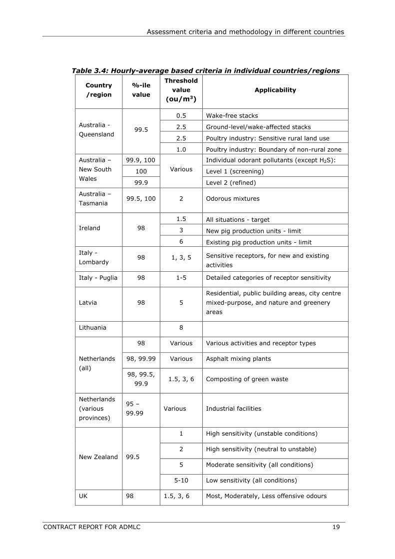
Table 3.4: Hourly-average based criteria in individual countries/regions
Country
/region
%-ile
value
Threshold
value
(ou/m3)
Applicability
Australia -
Queensland 99.5
0.5 Wake-free stacks
2.5 Ground-level/wake-affected stacks
2.5 Poultry industry: Sensitive rural land use
1.0 Poultry industry: Boundary of non-rural zone
Australia –
New South
Wales
99.9, 100
Various
Individual odorant pollutants (except H2S):
100 Level 1 (screening)
99.9 Level 2 (refined)
Australia –
Tasmania 99.5, 100 2 Odorous mixtures
Ireland 98
1.5 All situations - target
3 New pig production units - limit
6 Existing pig production units - limit
Italy -
Lombardy 98 1, 3, 5 Sensitive receptors, for new and existing
activities
Italy - Puglia 98 1-5 Detailed categories of receptor sensitivity
Latvia 98 5
Residential, public building areas, city centre
mixed-purpose, and nature and greenery
areas
Lithuania 8
Netherlands
(all)
98 Various Various activities and receptor types
98, 99.99 Various Asphalt mixing plants
98, 99.5,
99.9 1.5, 3, 6 Composting of green waste
Netherlands
(various
provinces)
95 –
99.99 Various Industrial facilities
New Zealand 99.5
1 High sensitivity (unstable conditions)
2 High sensitivity (neutral to unstable)
5 Moderate sensitivity (all conditions)
5-10 Low sensitivity (all conditions)
UK 98 1.5, 3, 6 Most, Moderately, Less offensive odours
20 CONTRACT REPORT FOR ADMLC
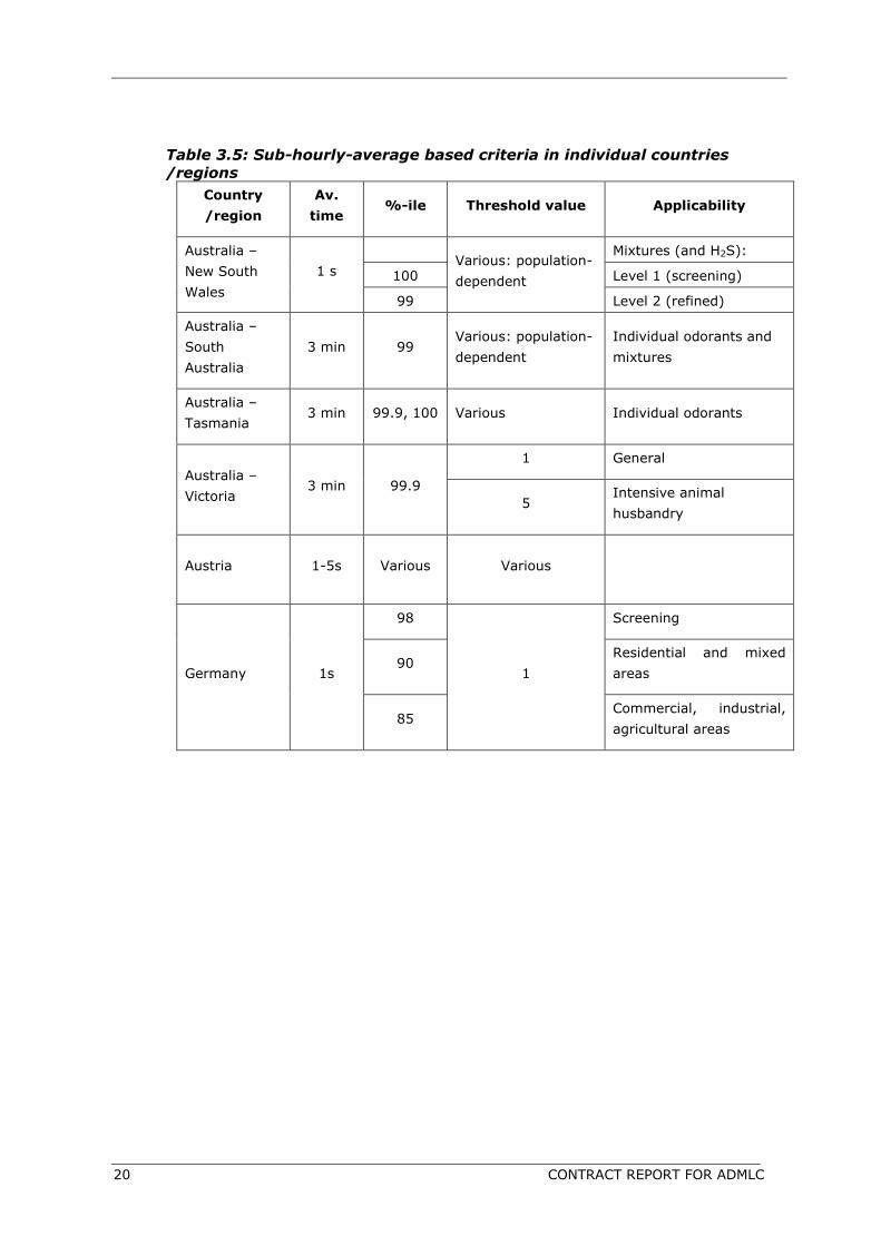
Table 3.5: Sub-hourly-average based criteria in individual countries
/regions
Country
/region
Av.
time %-ile Threshold value Applicability
Australia –
New South
Wales
1 s
Various: population-
dependent
Mixtures (and H2S):
100 Level 1 (screening)
99 Level 2 (refined)
Australia –
South
Australia
3 min 99 Various: population-
dependent
Individual odorants and
mixtures
Australia –
Tasmania 3 min 99.9, 100 Various Individual odorants
Australia –
Victoria 3 min 99.9
1 General
5 Intensive animal
husbandry
Austria 1-5s Various Various
Germany 1s
98
1
Screening
90 Residential and mixed
areas
85 Commercial, industrial,
agricultural areas
Models used for odour assessment
CONTRACT REPORT FOR ADMLC 21
4 MODELS USED FOR ODOUR ASSESSMENT
4.1 Gaussian Plume models
Gaussian plume models are routinely used for odour modelling and other regulatory
modelling. In their default mode of operation, they use a ‘steady-state’ approximation
and the pollutant concentrations display a normal (Gaussian) probability distribution about
the plume centreline.
Gaussian plume models are sometimes criticised as being simplistic and unable to treat
complex effects such as terrain and coastal effects; it is important to recognise and make
a distinction between the older Gaussian plume models such as ISCST3 and AUSPLUME
and newer, ‘advanced’ Gaussian Plume models such as ADMS and AERMOD where the
description of the atmospheric boundary layer is more advanced and complex effects may
be included.
4.2 Lagrangian models
Lagrangian models are models in which the trajectory and properties of each particle or
puff within the plume are calculated according to the mean wind field data, with the
assumption that model input conditions are changing over the model domain and model
time step. Consequently, these models can use temporally- and spatially-varying
meteorological data.
Statistics of concentrations are often derived from the trajectories of all of the particles or
puffs within the model domain.
4.3 Examples of models commonly used for odour
dispersion modelling
ADMS
ADMS is an advanced Gaussian Plume model, developed in the United Kingdom by
Cambridge Environmental Research Consultants (CERC, 2016). It has an odour module,
which allows the modelling to be carried out using odour units. It includes a fluctuations
module that can be used to calculate sub-hourly concentration statistics (Davies et al,
1998). Allowing for fluctuations within the ‘instantaneous’ plume and plume meandering,
including intermittency, this model estimates the probability of exceedence of specified
concentration (odour) thresholds by assuming a distribution function that depends on the
modelled ensemble mean plume properties and the turbulence characteristics of the
ambient air.
A new model feature has been developed for the purposes of this project: this enables a
yes/no output for each modelled hour, to indicate whether each hour meets the criteria
for an odour hour. The user provides sub-hourly averaging time, percentile and odour
threshold values.
AERMOD
AERMOD is an advanced Gaussian Plume model, developed by the US Environmental
Protection Agency (USEPA, 2021). It is a regulatory model, listed as a ‘preferred’ model in
Appendix W of the ‘Guideline of Air Quality Models’ of the USEPA (USEPA, 2017). It is
widely used for odour dispersion modelling.

22 CONTRACT REPORT FOR ADMLC
AERMOD has two regulatory input data processors: AERMET, which is a pre-processor for
meteorological data pre-processor, and AERMAP, a pre-processor for its complex terrain
data.
AUSPLUME
AUSPLUME is a Gaussian Plume model, which was developed by the Environmental
Protection Agency of Victoria, Australia (Victoria, 2002). It was developed as an extension
of the ISC model.
AUSPLUME is no longer being actively developed, since, as of 2014, it is no longer
supported by Victoria EPA for regulatory purposes.
Further details are given in Section 3.2.
AUSTAL2000
AUSTAL (Janicke Consulting and UBA, 2014) is a Lagrangian particle model based on
LASAT. AUSTAL2000 was released by the German Environment Agency as the regulatory
model in 2000 and was extended to include odour modelling capabilities in 2004. The
odour version is known as AUSTAL2000G, where the ‘G’ represents ‘Geruch’, the German
word for ‘odour’.
Olesen et al (2005) describe how there were two options under consideration for dealing
with fluctuating odour concentrations when AUSTAL2000G was being developed: a
meandering plume model, and a simple empirical function based on an hourly averaged
concentration. The latter was chosen, with the fixed peak-to-mean factor of four
determined, based on sensitivity analysis and validation against field experiment and wind
tunnel data.
AODM
AODM (Austrian Odour Dispersion Model) consists of three modules (Piringer et al, 2007).
The first module is used to carry out emission calculations. The second module is the
Austrian Gaussian regulatory dispersion model, which calculates hourly or 30-minute
average concentrations. The third module is used for the conversion of results to
‘instantaneous’ values, which varies according to the stability of the atmosphere.
CALPUFF
CALPUFF is developed by Exponent, Inc, and is a US Environmental Protection Agency
(EPA) ‘alternative model’ (USEPA, 2021). It is a non-steady-state puff dispersion model.
It runs using temporally- and spatially-varying meteorological data, and hence is
particularly designed for use on scales of tens to hundreds of kilometres.
CALPUFF includes some functionality in predicting sub-hour concentrations. The user guide
states that “A simple averaging-time scaling factor can be used to estimate short-term
peak concentrations for applications such as assessing the perception of odor.” “This
adjustment primarily addresses the effect of meandering (fluctuations in the wind about
the mean flow for the hour) on the average lateral distribution of material.”
GRAL
The Graz Lagrangian Model, or GRAL, (Oettl, 2021) was developed in 1999, in response
to a requirement for a model that could be used with the conditions of low wind speed
experienced for a large proportion of the time in the alpine areas of Austria. It is a
Lagrangian particle model.
It is widely used in a regulatory context, and includes the ability to calculate odour hours,
using a concentration-variance model, as further described in Section 7.2.3 of this report.
It is also possible to calculate odour hours by means of a fixed peak-to-mean value of
four, in line with the method used by AUSTAL2000.
OML
Operationelle Meteorologiske Luftkvalitetsmodeller, or OML, is a modern Gaussian plume
model, developed at the Danish National Environmental Research Institute NERI and

Models used for odour assessment
CONTRACT REPORT FOR ADMLC 23
hosted by Aarhus University (Aarhus University, 2021). It is a regulatory model and is
widely used in Denmark.
LASAT
Lagrange Simulation of Aerosol Transport, or LASAT, is a German Lagrangian particle
dispersion model, developed by Janicke Consulting (Janicke Consulting, 2021). It provided
the basis for the development of the AUSTAL2000 model.
24 CONTRACT REPORT FOR ADMLC
5 VALIDATION STUDIES
5.1 Measurement methods used in odour model validation
studies
In order to interpret and understand the results of dispersion modelling validation studies,
it is useful to introduce the main measurement methods used for comparison purposes.
Historically, validation of odour dispersion modelling has met with a fundamental
challenge, in that the quantification of odour in the environment is very difficult. The
human olfactory system is, clearly, an efficient detector system, but there are challenges
with standardisation. The technique of dynamic olfactometry is a standardised method,
but this was developed for the quantification of odour emission concentrations at, or very
close to, the source; the consequence is that dynamic olfactometry is more suitable for
measuring odour concentrations that are typically well in excess of the human detection
thresholds under ambient conditions.
Other validation studies compare the dispersion model results against odour complaint
records, questionnaires and other similar ‘community’ based databases.
Experiments employing inert tracer gases, both in the field and in wind tunnels also
represent an important resource for odour model validation. Capelli et al (2013), for
example, highlight the value of these types of experiments in odour dispersion modelling
validation. Full scale tracer experiments carried out for the purposes of odour research
have been conducted in conjunction with ambient odour measurements.
There have been recent advances in the measurement of odours in the environment
including ‘electronic noses’ and standardised human panel measurements (Capelli et al,
2013).
An important development in the advancement of field measurements by human panels is
the publication of the EN 16841 European Standard in 2017 (CEN, 2016a; CEN, 2016b).
This is made up of two parts, each describing a specific method:
EN 16841-1 - grid method
EN 16841-2 - plume method
Both methods rely on a minimum of eight carefully selected panel members, qualified (in
terms of acuity) according to the EN 13725 standard (CEN, 2003).
The aim of the grid method is to determine the frequency of odour exposure within a
defined area, with measurements of sufficient duration to cover a representative sample
of meteorological conditions. Panel members are distributed over a grid system. Odour is
determined on a 10-second basis, over measurement periods of 10 minutes.
The aim of the plume method is to determine the extent of the odour plume. Panel
members traverse the general area of the odour plume in a zig-zag manner, giving a
yes/no response to indicate the presence/absence of odour and therefore delineate the
‘edges’ of the plume.
The methodology provides a consistent approach across the European member states, and
possibly in other areas of the world that follow this or similar methodologies.
The grid method is, at least in theory, highly suited to the assessment of the odour hour
criteria. Oettl et al (2018a) point out, however, that the method is very expensive in terms
of the number of people involved and time required for the inspections. In addition,
Brancher et al (2019) suggest that the ‘recognisable’ odour is “ambiguously defined”.
The plume method has essentially been used in Belgium for several years in conjunction
with subsequent reverse dispersion modelling (although the reverse dispersion modelling
Validation studies
CONTRACT REPORT FOR ADMLC 25
is not part of the European Standard). Van Elst and Delva (2016) outline the pros and
cons of this plume extent measurement/reverse dispersion modelling methodology. They
point out that it is a simple method that is easily explained, and does not need
sophisticated equipment; is inexpensive; inherently accounts for different source types
and multiple sources; reflects the actual experience of ambient odours, as opposed to an
experience in an artificial laboratory environment, and avoids the potential errors
introduced by the use of sample bags; and has potential to provide collective
understanding and feedback regarding an odour problem. As downsides to the method,
they highlight: the problems of inaccessible areas such as water bodies and privately-
owned areas; the likely inability to distinguish between different types of odour sources in
a given area; and the limitation of use in certain meteorological conditions, with only
specific conditions being suitable for clearly defining a plume extent.
In terms of the use of the EN 16841 standard (CEN 2016a; CEN 2016b) field inspection
data for dispersion model validation, an important consideration is that neither of the two
parts of the standard includes the measurement of the intensity of ambient odours; there
is no capacity for direct comparison with modelled concentrations, and the methods will
therefore be of limited use for model validation.
5.2 Selected validation studies
As noted by Capelli et al (2013), amongst others, there are relatively few studies that
specifically and robustly tackle the question of the validation of odour dispersion modelling.
This section of the report outlines the findings of a range of validation studies that have
been carried out. Table 5.1 provides an overview of these validation studies, and the main
features and findings of each of these studies are discussed below. A short discussion of
the main trends and common findings is given in Section 5.2.1 and further discussion is
given in Section 7.1.3.

26 CONTRACT REPORT FOR ADMLC
Table 5.1: Summary of selected published validation studies
Reference Sector Source type Receptor distance Measurement
type
Models
Baumann-
Stanzer et al
n/a
(validation
datasets)
OROD
(field) Point
Two transects: 150 m
and 275 m
Field inspection and
tracer
measurements ONG, ADMS, LASAT
MUST (wind
tunnel
data)
Point < 200 m Wind tunnel
experiments
Bull and
Fromant
Wastewater treatment Not known Up to 1 km Complaints record ADMS
Capelli and
Sironi Landfill Area
Close (up to few
hundred metres)
Field inspection
EN 16841 -2
(plume)
CALPUFF
Carpentieri
et al Landfill Elevated area source < 600 m
Wind tunnel
experiments
SAFE_AIR, ISC3 and
‘Van Ulden model’
Chirmata
and Ichou Fishing port Not known Up to 15 km Electronic nose
AERMOD
Dourado et
al Pig farm (CEDVAL) Point (stack) < 300m
Wind tunnel
experiments
A Gaussian
fluctuating plume
model
Drew et al Landfill Point and area Up to 10 km Human ‘community
monitors’
ADMS
Elbir et al Meat rendering Point (stack) 250 m and 500 m Olfactometry CALPUFF
Henry et al Pig farm Not known Not known
Several methods of
ambient field
measurement
AERMOD and
CALPUFF
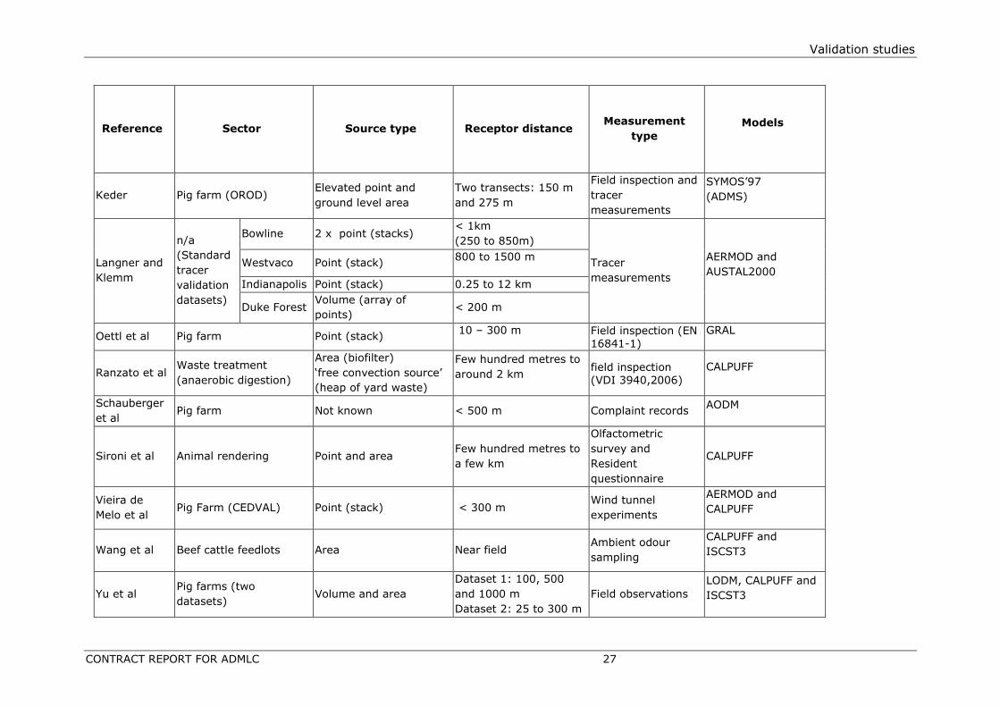
Validation studies
CONTRACT REPORT FOR ADMLC 27
Reference Sector Source type Receptor distance Measurement
type
Models
Keder Pig farm (OROD) Elevated point and
ground level area
Two transects: 150 m
and 275 m
Field inspection and
tracer
measurements
SYMOS’97
(ADMS)
Langner and
Klemm
n/a
(Standard
tracer
validation
datasets)
Bowline 2 x point (stacks) < 1km
(250 to 850m)
Tracer
measurements
AERMOD and
AUSTAL2000 Westvaco Point (stack)
800 to 1500 m
Indianapolis Point (stack) 0.25 to 12 km
Duke Forest Volume (array of
points) < 200 m
Oettl et al Pig farm Point (stack) 10 – 300 m Field inspection (EN
16841-1)
GRAL
Ranzato et al Waste treatment
(anaerobic digestion)
Area (biofilter)
‘free convection source’
(heap of yard waste)
Few hundred metres to
around 2 km field inspection (VDI 3940,2006)
CALPUFF
Schauberger
et al Pig farm Not known < 500 m Complaint records
AODM
Sironi et al Animal rendering Point and area Few hundred metres to
a few km
Olfactometric
survey and
Resident
questionnaire
CALPUFF
Vieira de
Melo et al Pig Farm (CEDVAL) Point (stack) < 300 m
Wind tunnel
experiments
AERMOD and
CALPUFF
Wang et al Beef cattle feedlots Area Near field Ambient odour
sampling
CALPUFF and
ISCST3
Yu et al Pig farms (two
datasets) Volume and area
Dataset 1: 100, 500
and 1000 m
Dataset 2: 25 to 300 m
Field observations
LODM, CALPUFF and
ISCST3

28 CONTRACT REPORT FOR ADMLC
Baumann-Stanzer et al (2008) compared LASAT, ADMS and ONG (a simple Gaussian
plume model) against two field experiment datasets. The first set of experiments were
field experiments from the OROD project, and the second set were wind tunnel data from
the Mock Urban Setting Test (MUST) project. They found varying levels of agreement with
different experiments. They highlight the importance of the general model setup and
ensuring that the terrain and roughness characteristics are effectively described by the
user and treated by the model.
Bull and Fromant (2014) carried out dispersion modelling for 15 wastewater treatment
works (WwTW) sites in the UK, using ADMS to calculate the 98th percentile of hourly
average concentrations, and investigated the relationship between the modelled
concentrations and reported complaints around the sites. The model output was split into
concentration bands (1.5 – 3, 3 – 5 and > 5 ouE/m3).
The study found that odour modelling results did not correlate well with the location of the
reported complaints and that the 98th percentile of hourly average concentrations
calculated in the modelling underestimated the area over which complaints would be
expected, in most cases. The authors discussed the most likely reasons for this lack of
correlation. The main issue that they identify is that, in lieu of more specific data, the
dispersion modelling was carried out using fixed, generic, odour emission rates. They used
‘typical’ values which were industry-standard values representing normal operations at
WwTW sites, and the authors recognised the significant problem with this, in that
complaints are likely to occur during periods when emissions are not at typical levels.
Another major issue discussed was problems with the complaints record; they highlighted
that it spanned several years, over which time many factors were thought to influence
complaint patterns, including targeted campaign periods, where residents were urged to
make complaints. When they removed ‘anomalous’ years the correlation improved, albeit
modestly.
Capelli and Sironi (2018) modelled a landfill using CALPUFF and compared the results with
field inspection results using the EN 16841-2 (plume) method (CEN 2016b). They modelled
the landfill as an area source, using two different methods for the odour emission rate;
the first assumed a wind speed-dependent emission rate, and the second a constant
emission rate. When modelling with the first approach, they found that the model results
significantly overestimated the results from the field inspection measurements. This is
despite their belief that the constant peak-to-mean value of 2.3 used is too low for the
short downwind distances involved in the assessment. They report that a constant
emission rate gave better results, with the extent and shape of the resulting plume giving
much better agreement with the field inspection results. Furthermore, they found that
significantly reducing the fixed emission rate (originally determined using a wind tunnel
and olfactometry) gave even better agreement with the field measurements. They note
that odour emission rate measurements using a wind tunnel tend to overestimate emission
rates from low-emissive sources such as the surfaces of landfill sites, and that wind-
dependent emission rates have been shown elsewhere to be inappropriate for modelling
landfill sites. This is because the main mechanism for volatilisation of the odorous
compounds is not forced convection at the surface, but an upwards flow of gas that has
already formed within the landfill structure. They note that this is relevant, as this method
of applying variable emission rates to landfill sources had been proposed in the Lombardy
region of Italy.
Carpentieri et al (2008) carried out a validation exercise based on wind tunnel experiments
of emissions from an elevated area source, representing emissions from a landfill located
on a hill. They used three dispersion models: SAFE_AIR, ISC3 and a model code based on
work of by Van Ulden. They found that the agreement of the modelling results with the
wind tunnel experiments was not as good as is generally found with a simpler source
configuration, that is a single stack point source. The best agreement for these

Validation studies
CONTRACT REPORT FOR ADMLC 29
assessments was with the Van Ulden code; SAFE_AIR performed reasonably well, and the
least good agreement was with ISC3.
Chirmata and Ichou (2016) modelled a fishing port, including odour sources such as fish
waste transfer, and fish trading activities, and compared the results with continuous
electronic nose measurements. They note that the peak measured odour concentrations
tended to occur when wind speeds were less than 2 m/s. They also found that the peak
concentrations output from the modelling, carried out using AERMOD, tended to be lower
than the peak measured concentrations.
Dourado et al (2013) carried out a validation of a fluctuating Gaussian plume model, FPM,
developed to take into account concentration peaks and the intermittency factor and
frequency of the odour events. Results were compared with the CEDVAL wind tunnel
dataset and also compared to results obtained from CFD modelling. They found good
general agreement, but identified a consistent tendency for both the fluctuating plume and
CFD models to overpredict the concentrations from the wind tunnel experiments.
Drew et al (2007) modelled sources at a landfill site using ADMS and compared modelled
results with several years of monitoring data from volunteer members of the surrounding
community, and some complaint records, based on the 98th percentile of hourly average
concentrations. They found that there was good correlation only when averaging times
shorter than an hour were used for the model output concentrations; this effectively meant
that the hourly average output concentrations were not high enough to predict the odour
nuisance.
Elbir et al (2007) modelled odours from a meat packaging and rendering plant using
CALPUFF and compared the modelled values with ambient concentrations, measured using
olfactometry, at two sites, 250 m and 500 m downwind from the odour source, which
comprised a 16 m stack, with an efflux temperature of 40°C. This dataset is notable
because of the inclusion of measurements over short averaging times (a frequency of 20
s and sampling duration of 10 s), with accompanying high frequency wind speed and
direction measurements. The total duration of each measurement period was ten minutes.
Meteorological conditions were measured onsite, at the same frequency as the odour
sampling. The atmospheric conditions were slightly stable.
They used the power law equation method for peak-to-mean conversion from one hour to
shorter averaging times. They ran CALPUFF for each of the wind speed and direction values
(once for each 20-second meteorological data period) and applied the peak-to-mean
adjustment to that value. They found that there was good agreement between the
measured and modelled results.
Henry et al (2010) modelled swine finishing barns in Iowa, using CALPUFF and AERMOD.
Ambient odour concentrations were measured using four different techniques. They found
that the results obtained using AERMOD generally gave slightly better agreement with the
measurements than those using CALPUFF. They found, however, that there was a wide
variation in the results from the different ambient measurement techniques.
Keder (2008) used the Czech model, SYMOS’97 to carry out modelling, and compared the
model results with measurements from the BWPLUS (OROD) dataset (as described in
Section 6.3) and with results from modelling carried out using ADMS. Their findings were
that there was generally good agreement between the modelled and observed
concentrations. Compared with ADMS, SYMOS appeared to underestimate the area of
odour impact, especially for ground level area sources. Ground level peak odour
concentrations were mostly lower in SYMOS compared with the ADMS results. It is
suggested that the results from SYMOS may be improved by changing the peak-to-mean
ratios used in the SYMOS calculations.
30 CONTRACT REPORT FOR ADMLC
Langner and Klemm (2011) compared output from AERMOD and AUSTAL2000 with data
from five standard field experiment datasets. They concluded that they consider AERMOD
to be more suitable for modelling odour, as it gave better agreement with field
measurements for most of the modelled cases and performed well overall. They found that
AUSTAL tended to underpredict impacts, particularly during stable conditions. They found
that AERMOD results gave better agreement than AUSTAL when terrain or urban effects
were modelled; for simple terrain and surface characteristics, both models performed
equally well.
Oettl et al (2018a) carried out dispersion modelling using GRAL and compared the model
output with data from measurements carried out by field inspection, using the EN 16841-
1 (grid) method (CEN 2016a). They used GRAL in two different ways: a) Using a
concentration-variance method within GRAL especially designed for calculating odour
hours and b) Applying a fixed peak-to-mean value of 4 to standard hourly average
concentrations output from GRAL. They stressed that results using the concentration
variance version of GRAL could give good agreement with the EN 16841-1 method, but
that taking into account the variation of individual odour sensitivities of qualified panel
members is very important in selecting an appropriate odour model. They found that
applying the modelling method involving a fixed peak-to-mean value of 4 led to an
overestimation of odour in most cases.
Ranzato et al (2012) used CALPUFF to model an anaerobic digestion site in Italy and
compared the results against extensive measurements taken over a six-month period
using the VDI 3940 Field inspection method, the German regulatory field inspection
standard. This was a test of the German regulatory ‘odour hour’ criteria, including
consideration of local complaint information. Overall they found good general agreement
between the two methods in terms of defining the spatial extent of odour
annoyance/nuisance. When comparing results at individual receptor locations, the
agreement was generally good, and they conclude that they support the application of
both the field inspection and the modelling methods. They found, however, that the model
outputs tended to underestimate peak concentrations close to the source; they suggest
that this may be because it was not possible to replicate fugitive emissions in CALPUFF, or
that an inappropriate peak-to-mean ratio was used. (they multiplied output hourly values
by a peak-to mean factor of 1.58). Another interesting finding was that the difference
between the model output and measurements was particularly large when the field
inspection results equated to zero frequencies of odour. They suggest that this might be
due to the much shorter time period represented in the field assessment measurements,
or perhaps because of the linear additive nature of the odour concentrations from different
source types in CALPUFF, which might not be the case in reality, and could therefore lead
to overestimates in the model results.
Schauberger et al (2001) compared output from AODM with data from odour complaint
records, for emissions from a pig farm. They found a disagreement with the timings of the
odour complaints compared with the model outputs. The periods with the greatest number
of complaints were early mornings and late at night, High levels of complaints were also
found to correspond to periods of transition between day and night, with stable
stratification near the ground. They had several suggestions of possible reasons for this
discrepancy. Their first suggestion is that the behaviour of the complainants was not taken
into account; i.e. the greater potential for complaints at specific times of the day and times
of the year. Interestingly, they suggest that odour should be weighted by the time of day
and seasonally, in a similar manner to noise criteria. Their second suggestion is that the
modelling did not take into account the variations in the odour emission caused by changes
in temperature, ventilation rate, animal activity, etc. They found that, for the prevailing
wind direction, odour episodes only occurred during neutral and slightly unstable
atmospheric conditions.
Validation studies
CONTRACT REPORT FOR ADMLC 31
Sironi et al (2010) carried out modelling using CALPUFF, in Lombardy, Italy, for four
rendering plants located in close proximity to one another. The modelled output was
compared against data from social participation in the form of questionnaires.
Olfactometric surveys were used to inform the emission data. It is interesting to note that
they multiplied output hourly values by a peak-to-mean factor of 2.3, and then took the
98th percentile of the resulting peak concentrations, in accordance with the specific
guidance for the region of Lombardy. A threshold of 1 ouE/m3 was used when determining
whether the modelled concentrations constituted an odour incidence. They found very
good overall correlation between the odour incidence reported in the questionnaires and
the modelled odour concentrations.
Vieira de Melo et al (2012) used AERMOD and CALPUFF for a validation study using the
CEDVAL dataset. They found that, overall, the results from the AERMOD modelling gave
better agreement in the near field than those from the CALPUFF modelling, and the
CALPUFF results gave better agreement further downwind.
Wang et al (2006) compared output from CALPUFF and the ISCST3 model when modelling
a commercial beef cattle feedlots farm and found that while CALPUFF results agreed
reasonably well with the experimental data (odour measurements by panel members), the
ISCST3 results significantly underestimated the impacts. They also found that both the
CALPUFF and ISCST3 model output did not replicate peak odour concentrations, when
using a constant average emission rate.
Yu et al (2011) carried out a study of two livestock odour datasets using the Livestock
Odor Dispersion Model (LODM), and also modelled the same scenarios using the CALPUFF
and ISCST3 models. Both datasets comprised downwind field observations made by
trained human sniffers. Each measurement session comprised 10-second observations of
odour intensity and description, carried out for a total duration of ten minutes. The models
were run using hourly meteorological data and the results compared with the 10-minute
averaged field observations.
The first dataset consisted of measurements from two pig farms. Both of the farms
included mechanically-ventilated animal housing, modelled as volume sources in LODM
and area sources in the other two models. The farms also had earthen manure storage,
open on the first farm and covered on the second farm; both were modelled as area
sources in all models. The second dataset consisted of measurements from 28 farms,
covering a variety of different animals.
The main findings were that all three models generally gave similar results. The results
from LODM did not give very good agreement close to the sources, but gave better
agreement at locations further downwind. The researchers suggest that a key reason for
the discrepancy between measured and observed data may have been the process of
conversion of odour intensity observations to odour concentrations by means of a
logarithmic relationship They note that three such equations from different groups of
researchers gave very different concentrations.
5.2.1 Conclusions
While it is unfeasible to draw many definitive conclusions from the relatively small number
of robust studies available, due to the disparities in the model type, source type, odour,
measurement methodology and the level of detail available, there are some common
themes and patterns.
Many authors report that their modelling underpredicted the measured values, particularly
peak values, and values close to the sources. Notable exceptions are the modelling by
Dourado et al (2013), using a fluctuating Gaussian plume model and a CFD model, and
32 CONTRACT REPORT FOR ADMLC
the use of the fixed value of 4 for the peak-to-mean ratio by Oettl et al (2018a) where
there was a tendency to overestimate concentrations.
Where authors report good agreement with peak concentrations, this is often achieved by
changing the peak-to-mean ratio for conversion from hourly averages.
It was frequently noted that the modelling of fugitive emissions was especially challenging.
There was particular concern about the degree to which the emission rate measurements
were representative of the emissions, including temporal variability in emission rates.
There was also a general consensus that the key aspects of the model setup, such as
topography, building effects and surface roughness can have significant effects on model
results, and the sensitivity of the results to these features should be taken into
consideration.
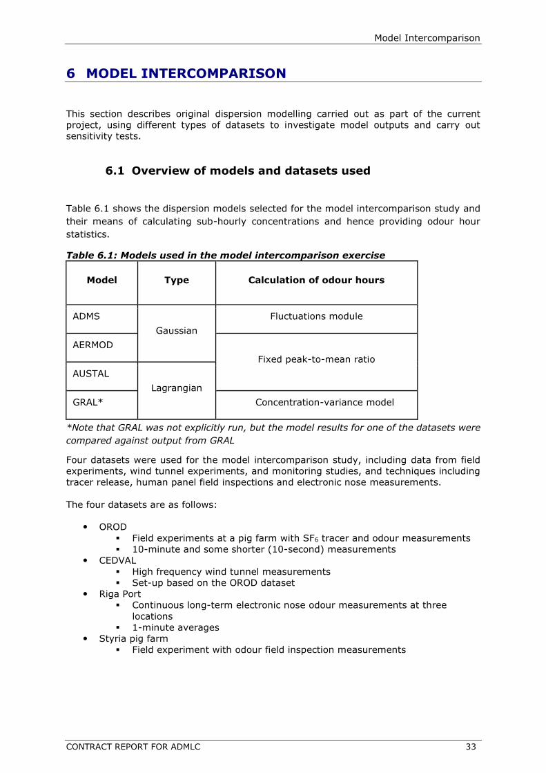
Model Intercomparison
CONTRACT REPORT FOR ADMLC 33
6 MODEL INTERCOMPARISON
This section describes original dispersion modelling carried out as part of the current
project, using different types of datasets to investigate model outputs and carry out
sensitivity tests.
6.1 Overview of models and datasets used
Table 6.1 shows the dispersion models selected for the model intercomparison study and
their means of calculating sub-hourly concentrations and hence providing odour hour
statistics.
Table 6.1: Models used in the model intercomparison exercise
Model Type Calculation of odour hours
ADMS
Gaussian
Fluctuations module
AERMOD
Fixed peak-to-mean ratio
AUSTAL
Lagrangian
GRAL* Concentration-variance model
*Note that GRAL was not explicitly run, but the model results for one of the datasets were
compared against output from GRAL
Four datasets were used for the model intercomparison study, including data from field
experiments, wind tunnel experiments, and monitoring studies, and techniques including
tracer release, human panel field inspections and electronic nose measurements.
The four datasets are as follows:
OROD
▪ Field experiments at a pig farm with SF6 tracer and odour measurements
▪ 10-minute and some shorter (10-second) measurements
CEDVAL
▪ High frequency wind tunnel measurements
▪ Set-up based on the OROD dataset
Riga Port
▪ Continuous long-term electronic nose odour measurements at three
locations
▪ 1-minute averages
Styria pig farm
▪ Field experiment with odour field inspection measurements

34 CONTRACT REPORT FOR ADMLC
6.2 OROD dataset
6.2.1 General experimental setup
This dataset was created as part of the BWPLUS program, and is described and presented
in detail in a research report (Bachlin et al, 2002). The dataset comprises 14 tracer and
odour dispersion experiments carried out over three days, around an isolated pig barn on
a farm near the town of Biberach in Germany, in a rural area with flat terrain. The site is
the same as that replicated in the ‘CEDVAL Wind tunnel experiments’ dataset (described
in Section 6.3).
The focus of the experiments was a single emission point on the roof of the pig barn. In
addition to the existing pig odour emissions, a tracer gas, sulphur hexafluoride (SF6) was
also released from the emission point, and simultaneous ambient measurements of both
odour and SF6 were carried out, at an array of points downwind of the emission point. The
ambient odour was measured in-situ by human assessors, and air samples were taken,
for the measurement of the ambient SF6 concentrations.
Each of the 14 experiments were of 10-minute duration, with the ambient measurements
representing both 10-minute and 10-second exposure durations. Simultaneous onsite
meteorological measurements were also carried out.
The philosophy behind these experiments is that “the generation of validation data sets
should include not only the odour, but also the propagation of another gas detectable by
physical measuring instruments in order to be able to more clearly compare the results
from field experiments and dispersion calculations”.
Emissions
The ventilation system of the pig barn consisted of underfloor extraction via two large
exhaust ducts each ending in a stack on the roof of the barn. During the experiments, the
ventilation system was deliberately set up so that only one exhaust duct/stack was
operating; the fan in the other exhaust duct was switched off and the opening was closed.
Air samples were taken directly from the air flow of the operating exhaust duct in order to
quantify the odour emission concentrations, using olfactometry measurements. The SF6
was released via the same exhaust duct; it was introduced directly into the exhaust air
flow and hence released to the atmosphere via the stack. The amount released was
controlled and measured using a flowmeter, and, as a check, random air samples were
also taken at the stack exit point to measure the SF6 emission concentrations.
The volume flow rate of the exhaust air was measured continuously. The flows were
relatively constant over the course of each experiment, and the small changes that did
occur were recorded.
Ambient measurements
The odour data and concentration data for the tracer were measured simultaneously and
at the same locations, over two transects running perpendicular to the generally south-
westerly wind, at 150 m and 275 m downwind of the exhaust duct. For some of the
experiments a single transect was used, and for others both transects were used.
For each experiment, several human ‘subjects’ were located along the transects at specific
monitoring locations, and 10-second average odour observations were measured at each
of these locations. The odour observations were carried out in accordance with the VDI
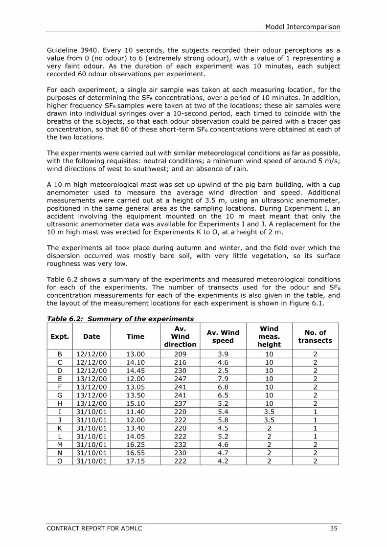
Model Intercomparison
CONTRACT REPORT FOR ADMLC 35
Guideline 3940. Every 10 seconds, the subjects recorded their odour perceptions as a
value from 0 (no odour) to 6 (extremely strong odour), with a value of 1 representing a
very faint odour. As the duration of each experiment was 10 minutes, each subject
recorded 60 odour observations per experiment.
For each experiment, a single air sample was taken at each measuring location, for the
purposes of determining the SF6 concentrations, over a period of 10 minutes. In addition,
higher frequency SF6 samples were taken at two of the locations; these air samples were
drawn into individual syringes over a 10-second period, each timed to coincide with the
breaths of the subjects, so that each odour observation could be paired with a tracer gas
concentration, so that 60 of these short-term SF6 concentrations were obtained at each of
the two locations.
The experiments were carried out with similar meteorological conditions as far as possible,
with the following requisites: neutral conditions; a minimum wind speed of around 5 m/s;
wind directions of west to southwest; and an absence of rain.
A 10 m high meteorological mast was set up upwind of the pig barn building, with a cup
anemometer used to measure the average wind direction and speed. Additional
measurements were carried out at a height of 3.5 m, using an ultrasonic anemometer,
positioned in the same general area as the sampling locations. During Experiment I, an
accident involving the equipment mounted on the 10 m mast meant that only the
ultrasonic anemometer data was available for Experiments I and J. A replacement for the
10 m high mast was erected for Experiments K to O, at a height of 2 m.
The experiments all took place during autumn and winter, and the field over which the
dispersion occurred was mostly bare soil, with very little vegetation, so its surface
roughness was very low.
Table 6.2 shows a summary of the experiments and measured meteorological conditions
for each of the experiments. The number of transects used for the odour and SF6
concentration measurements for each of the experiments is also given in the table, and
the layout of the measurement locations for each experiment is shown in Figure 6.1.
Table 6.2: Summary of the experiments
Expt. Date Time
Av.
Wind
direction
Av. Wind
speed
Wind
meas.
height
No. of
transects
B 12/12/00 13.00 209 3.9 10 2
C 12/12/00 14.10 216 4.6 10 2
D 12/12/00 14.45 230 2.5 10 2
E 13/12/00 12.00 247 7.9 10 2
F 13/12/00 13.05 241 6.8 10 2
G 13/12/00 13.50 241 6.5 10 2
H 13/12/00 15.10 237 5.2 10 2
I 31/10/01 11.40 220 5.4 3.5 1
J 31/10/01 12.00 222 5.8 3.5 1
K 31/10/01 13.40 220 4.5 2 1
L 31/10/01 14.05 222 5.2 2 1
M 31/10/01 16.25 232 4.6 2 2
N 31/10/01 16.55 230 4.7 2 2
O 31/10/01 17.15 222 4.2 2 2
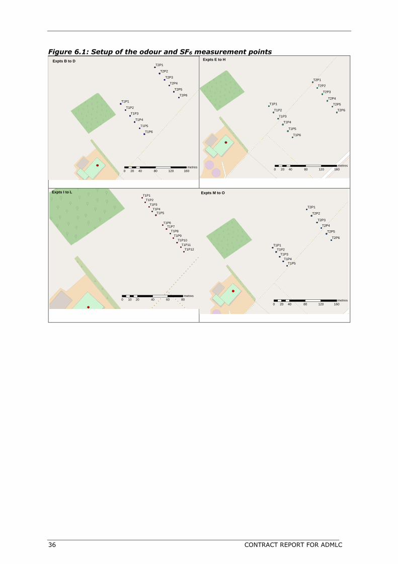
36 CONTRACT REPORT FOR ADMLC
Figure 6.1: Setup of the odour and SF6 measurement points
T2P6
T2P5
T2P4
T2P3
T2P2
T2P1
T1P6
T1P5
T1P4
T1P3
T1P2
T1P1
0 40 80 120 16020metres
Service Layer Credits: (c) OpenStreetMap and contributors, Creative Commons-Share Alike License (CC-BY-SA)
Expts B to D
T2P6
T2P5
T2P4
T2P3
T2P2
T2P1
T1P6
T1P5
T1P4
T1P3
T1P2
T1P1
0 40 80 120 16020metres
Service Layer Credits: (c) OpenStreetMap and contributors, Creative Commons-Share Alike License (CC-BY-SA)
Expts E to H
T2P6
T2P5
T2P4
T2P3
T2P2
T2P1
T1P5
T1P4
T1P3
T1P2
T1P1
0 40 80 120 16020metres
Service Layer Credits: (c) OpenStreetMap and contributors, Creative Commons-Share Alike License (CC-BY-SA)
Expts M to O
T1P9
T1P8
T1P7
T1P6
T1P5
T1P4
T1P3
T1P2
T1P1
T1P12
T1P11
T1P10
0 20 40 60 8010metres
Service Layer Credits: (c) OpenStreetMap and contributors, Creative Commons-Share Alike License (CC-BY-SA)
Expts I to L
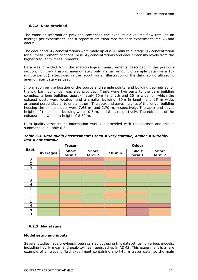
Model Intercomparison
CONTRACT REPORT FOR ADMLC 37
6.2.2 Data provided
The emission information provided comprised the exhaust air volume flow rate, as an
average per experiment, and a separate emission rate for each experiment, for SF6 and
odour.
The odour and SF6 concentrations were made up of a 10-minute average SF6 concentration
for all measurement locations, plus SF6 concentrations and odour intensity levels from the
higher frequency measurements.
Data was provided from the meteorological measurements described in the previous
section. For the ultrasonic anemometer, only a small amount of sample data (for a 10-
minute period) is provided in the report, as an illustration of the data, so no ultrasonic
anemometer data was used.
Information on the location of the source and sample points, and building geometries for
the pig barn buildings, was also provided. There were two parts to the barn building
complex: a long building, approximately 50m in length and 30 m wide, on which the
exhaust ducts were located; and a smaller building, 30m in length and 15 m wide,
arranged perpendicular to one another. The apex and eaves heights of the longer building
housing the exhaust duct were 7.65 m, and 2.70 m, respectively. The apex and eaves
heights of the smaller building were 10.6 m, and 8 m, respectively. The exit point of the
exhaust duct was at a height of 8.50 m.
Data quality assessment information was also provided with the dataset and this is
summarised in Table 6.3.
Table 6.3: Data quality assessment: Green = very suitable, Amber = suitable,
Red = not suitable
Expt.
Tracer Odour
Averages Short
term 1
Short
term 2 10-min
Short
term 1
Short
term 2
B
C
D
E
F
G
H
I
J
K
L
M
N
O
6.2.3 Model runs
Model setup and inputs
Several studies have previously been carried out using this dataset, using various models,
including hourly mean and peak-to-mean approaches in ADMS. This experiment is a rare
example of a relevant field experiment containing short-term tracer data, so the main

38 CONTRACT REPORT FOR ADMLC
focus here is on comparing this data with sub-hourly concentration output, from the
fluctuations module in ADMS.
Model runs were carried out, for each of the experiments, for comparison against the 10-
second SF6 tracer data. The emissions were modelled as a point source, and Table 6.4
shows the modelled source parameters. The efflux temperature of the source was set to
‘ambient’ which means that the temperature in the meteorological data was used as the
efflux temperature. The volume flow rate and SF6 emission rate was varied for each of the
experiments, as per the data provided.
Fluctuations and building effects cannot be modelled together, so building effects were not
modelled. The modelled surface roughness length was 0.1 m.
Table 6.4: Modelled source parameters
Source
type Height (m) Diameter (m)
Volume
flow rate
(m3/s)
Exit
temperature
(°C)
SF6
emission
rate
Point 8.5 1.239 variable ambient variable
Results
Results are shown only for those experiments for which the data quality is described as
‘very suitable’ (see Table 6.3).
Figure 6.2 shows a comparison of the full range of percentiles of 10-second average
concentrations output from ADMS at the relevant measurement sites, compared with the
equivalent measured values, for several of the experiments. Taken as a whole the shape
of the percentile distributions are well represtend by the model. For Experiments F, G and
H there is a tendency for underprediction by ADMS, while there is significantly better
agreement for Experiments K and I.
Figure 6.3 shows the peak-to-mean values calculated by ADMS at the relevant
measurement sites, compared with those calculated from the measured data, where the
peak is the 90th percentile of 10-second averages. Note that the the H1 transect modelled
peak-to-mean value does not appear on the plot, as the 90th percentile value was zero.
Figure 6.4 shows quantile-quantile plots of the 10-minute mean concentrations, for model
runs with and without building effects included. This shows a similar pattern of
underprediction to that shown in Figure 7 of Brancher et al (2020b), who carried out model
runs for this dataset with the LASAT model. The authors also note that several studies
report that measured concentrations for this dataset are higher than modelled
concentrations. The CEDVAL wind tunnel measurement dataset, described in Section 6.3,
also shows a general pattern of concentrations that are lower than those of the measured
full scale OROD dataset (Aubrun and Leitl, 2004).
It is notable that the quantile-quantile plots suggest that the impacts of the buildings on
measured concentrations are relatively limited in most cases. Building effects are also
discussed by Brancher et al.

Model Intercomparison
CONTRACT REPORT FOR ADMLC 39
Figure 6.2: Percentiles of 10 s average concentrations from key experiments
Experiment F
Experiment G
Experiment H
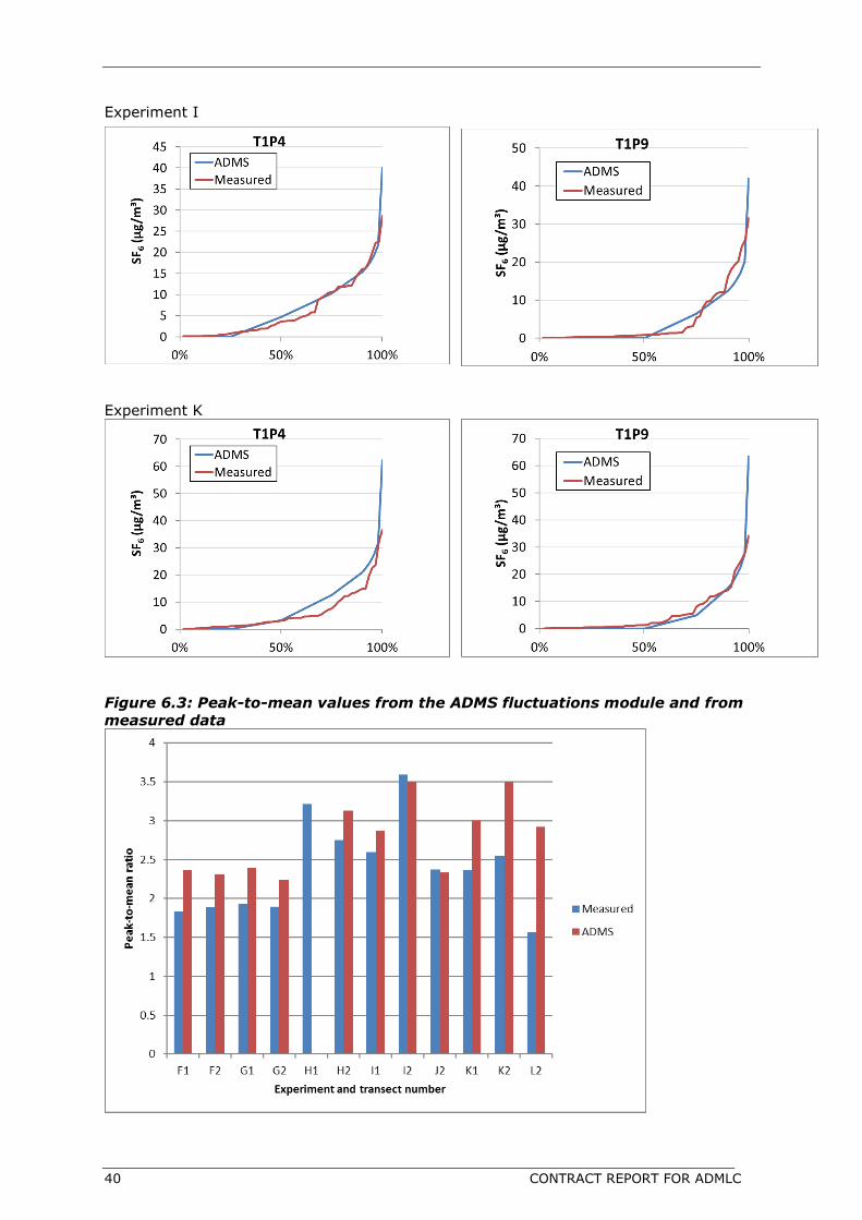
40 CONTRACT REPORT FOR ADMLC
Experiment I
Experiment K
Figure 6.3: Peak-to-mean values from the ADMS fluctuations module and from
measured data

Model Intercomparison
CONTRACT REPORT FOR ADMLC 41
Figure 6.4 Quantile-quantile plots of mean concentration for a) all results b)
near field only c) far field only
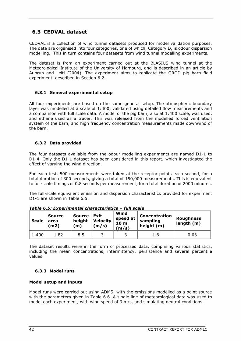
42 CONTRACT REPORT FOR ADMLC
6.3 CEDVAL dataset
CEDVAL is a collection of wind tunnel datasets produced for model validation purposes.
The data are organised into four categories, one of which, Category D, is odour dispersion
modelling. This in turn contains four datasets from wind tunnel modelling experiments.
The dataset is from an experiment carried out at the BLASIUS wind tunnel at the
Meteorological Institute of the University of Hamburg, and is described in an article by
Aubrun and Leitl (2004). The experiment aims to replicate the OROD pig barn field
experiment, described in Section 6.2.
6.3.1 General experimental setup
All four experiments are based on the same general setup. The atmospheric boundary
layer was modelled at a scale of 1:400, validated using detailed flow measurements and
a comparison with full scale data. A model of the pig barn, also at 1:400 scale, was used,
and ethane used as a tracer. This was released from the modelled forced ventilation
system of the barn, and high frequency concentration measurements made downwind of
the barn.
6.3.2 Data provided
The four datasets available from the odour modelling experiments are named D1-1 to
D1-4. Only the D1-1 dataset has been considered in this report, which investigated the
effect of varying the wind direction.
For each test, 500 measurements were taken at the receptor points each second, for a
total duration of 300 seconds, giving a total of 150,000 measurements. This is equivalent
to full-scale timings of 0.8 seconds per measurement, for a total duration of 2000 minutes.
The full-scale equivalent emission and dispersion characteristics provided for experiment
D1-1 are shown in Table 6.5.
Table 6.5: Experimental characteristics – full scale
Scale
Source
area
(m2)
Source
height
(m)
Exit
Velocity
(m/s)
Wind
speed at
10 m
(m/s)
Concentration
sampling
height (m)
Roughness
length (m)
1:400 1.82 8.5 3 3 1.6 0.03
The dataset results were in the form of processed data, comprising various statistics,
including the mean concentrations, intermittency, persistence and several percentile
values.
6.3.3 Model runs
Model setup and inputs
Model runs were carried out using ADMS, with the emissions modelled as a point source
with the parameters given in Table 6.6. A single line of meteorological data was used to
model each experiment, with wind speed of 3 m/s, and simulating neutral conditions.
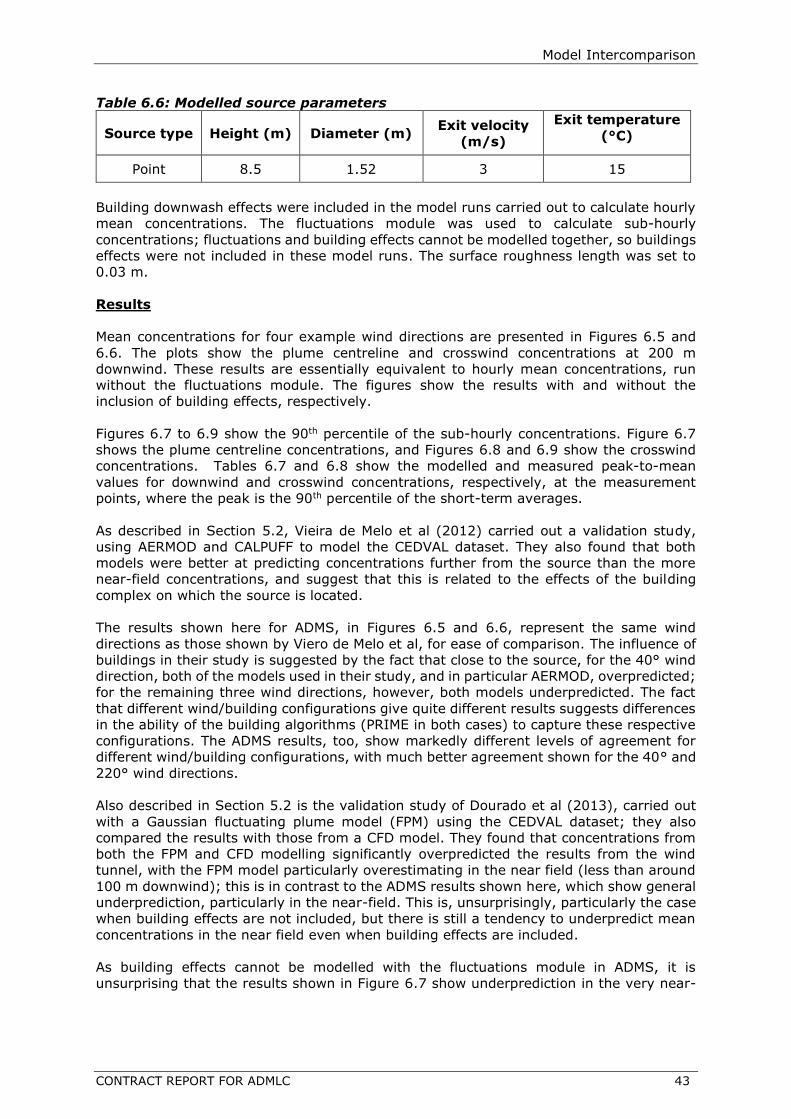
Model Intercomparison
CONTRACT REPORT FOR ADMLC 43
Table 6.6: Modelled source parameters
Source type Height (m) Diameter (m) Exit velocity
(m/s)
Exit temperature
(°C)
Point 8.5 1.52 3 15
Building downwash effects were included in the model runs carried out to calculate hourly
mean concentrations. The fluctuations module was used to calculate sub-hourly
concentrations; fluctuations and building effects cannot be modelled together, so buildings
effects were not included in these model runs. The surface roughness length was set to
0.03 m.
Results
Mean concentrations for four example wind directions are presented in Figures 6.5 and
6.6. The plots show the plume centreline and crosswind concentrations at 200 m
downwind. These results are essentially equivalent to hourly mean concentrations, run
without the fluctuations module. The figures show the results with and without the
inclusion of building effects, respectively.
Figures 6.7 to 6.9 show the 90th percentile of the sub-hourly concentrations. Figure 6.7
shows the plume centreline concentrations, and Figures 6.8 and 6.9 show the crosswind
concentrations. Tables 6.7 and 6.8 show the modelled and measured peak-to-mean
values for downwind and crosswind concentrations, respectively, at the measurement
points, where the peak is the 90th percentile of the short-term averages.
As described in Section 5.2, Vieira de Melo et al (2012) carried out a validation study,
using AERMOD and CALPUFF to model the CEDVAL dataset. They also found that both
models were better at predicting concentrations further from the source than the more
near-field concentrations, and suggest that this is related to the effects of the building
complex on which the source is located.
The results shown here for ADMS, in Figures 6.5 and 6.6, represent the same wind
directions as those shown by Viero de Melo et al, for ease of comparison. The influence of
buildings in their study is suggested by the fact that close to the source, for the 40° wind
direction, both of the models used in their study, and in particular AERMOD, overpredicted;
for the remaining three wind directions, however, both models underpredicted. The fact
that different wind/building configurations give quite different results suggests differences
in the ability of the building algorithms (PRIME in both cases) to capture these respective
configurations. The ADMS results, too, show markedly different levels of agreement for
different wind/building configurations, with much better agreement shown for the 40° and
220° wind directions.
Also described in Section 5.2 is the validation study of Dourado et al (2013), carried out
with a Gaussian fluctuating plume model (FPM) using the CEDVAL dataset; they also
compared the results with those from a CFD model. They found that concentrations from
both the FPM and CFD modelling significantly overpredicted the results from the wind
tunnel, with the FPM model particularly overestimating in the near field (less than around
100 m downwind); this is in contrast to the ADMS results shown here, which show general
underprediction, particularly in the near-field. This is, unsurprisingly, particularly the case
when building effects are not included, but there is still a tendency to underpredict mean
concentrations in the near field even when building effects are included.
As building effects cannot be modelled with the fluctuations module in ADMS, it is
unsurprising that the results shown in Figure 6.7 show underprediction in the very near-

44 CONTRACT REPORT FOR ADMLC
field. Much better agreement is demonstrated at 100 m and 200 m downwind, as shown
in Figures 6.8 and 6.9.
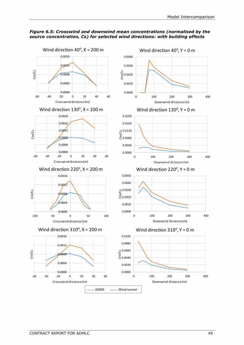
Model Intercomparison
CONTRACT REPORT FOR ADMLC 45
Figure 6.5: Crosswind and downwind mean concentrations (normalised by the
source concentration, Cs) for selected wind directions: with building effects
0.0000
0.0004
0.0008
0.0012
0.0016
-60 -40 -20 0 20 40 60
Cm
/Cs
Crosswind distance (m)
Wind direction 400, X = 200 m
Modelled Wind Tunnel
0.0000
0.0010
0.0020
0.0030
0.0040
0 100 200 300 400
Cm
/Cs
Downwind distance (m)
Wind direction 400, Y = 0 m
Modelled Wind Tunnel
0.0000
0.0040
0.0080
0.0120
0.0160
0.0200
0 100 200 300 400
Cm
/Cs
Downwind distance (m)
Wind direction 1300, Y = 0 m
Modelled Wind Tunnel
0.0000
0.0010
0.0020
0.0030
0.0040
0.0050
0 100 200 300 400
Cm
/Cs
Downwind distance (m)
Wind direction 2200, Y = 0 m
Modelled Wind Tunnel
0.0000
0.0020
0.0040
0.0060
0.0080
0.0100
0 100 200 300 400
Cm
/Cs
Downwind distance (m)
Wind direction 3100, Y = 0 m
Modelled Wind Tunnel
0.0000
0.0004
0.0008
0.0012
0.0016
0.0020
-60 -40 -20 0 20 40 60
Cm
/Cs
Crosswind distance (m)
Wind direction 1300, X = 200 m
Modelled Wind Tunnel
0.0000
0.0004
0.0008
0.0012
0.0016
-100 -50 0 50 100
Cm
/Cs
Crosswind distance (m)
Wind direction 2200, X = 200 m
Modelled Wind Tunnel
0.0000
0.0004
0.0008
0.0012
0.0016
-60 -40 -20 0 20 40 60
Cm
/Cs
Crosswind distance (m)
Wind direction 3100, X = 200 m
Modelled Wind Tunnel ADMS Wind tunnel
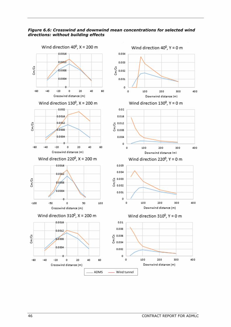
46 CONTRACT REPORT FOR ADMLC
Figure 6.6: Crosswind and downwind mean concentrations for selected wind
directions: without building effects
ADMS Wind tunnel
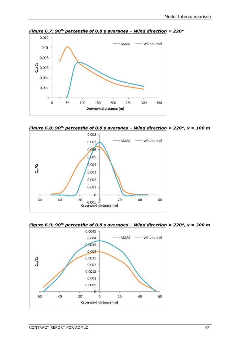
Model Intercomparison
CONTRACT REPORT FOR ADMLC 47
Figure 6.7: 90th percentile of 0.8 s averages – Wind direction = 220°
Figure 6.8: 90th percentile of 0.8 s averages – Wind direction = 220°, x = 100 m
Figure 6.9: 90th percentile of 0.8 s averages – Wind direction = 220°, x = 200 m

48 CONTRACT REPORT FOR ADMLC
Table 6.7: Downwind peak-to-mean ratios - Wind direction = 220 °
Downwind distance (m) Peak-to-mean ratio
ADMS Measured
50 0.3 2.4
75.2 4.0 2.4
100 4.0 2.4
200 3.4 2.1
300 3.4 2.0
Table 6.8: Crosswind peak-to-mean ratios - Wind direction = 220 °, x = 200 m
Crosswind distance (m) Peak-to-mean ratio
ADMS Measured
-56 - 2.3
-40 3.5 3.2
-28 4.0 2.6
-20 3.8 2.2
0 3.4 2.1
20 3.8 2.9
28 4.0 3.2
40 3.5 2.8
56 - 1.0
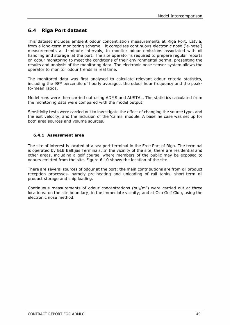
Model Intercomparison
CONTRACT REPORT FOR ADMLC 49
6.4 Riga Port dataset
This dataset includes ambient odour concentration measurements at Riga Port, Latvia,
from a long-term monitoring scheme. It comprises continuous electronic nose (‘e-nose’)
measurements at 1-minute intervals, to monitor odour emissions associated with oil
handling and storage at the port. The site operator is required to prepare regular reports
on odour monitoring to meet the conditions of their environmental permit, presenting the
results and analysis of the monitoring data. The electronic nose sensor system allows the
operator to monitor odour trends in real time.
The monitored data was first analysed to calculate relevant odour criteria statistics,
including the 98th percentile of hourly averages, the odour hour frequency and the peak-
to-mean ratios.
Model runs were then carried out using ADMS and AUSTAL. The statistics calculated from
the monitoring data were compared with the model output.
Sensitivity tests were carried out to investigate the effect of changing the source type, and
the exit velocity, and the inclusion of the ‘calms’ module. A baseline case was set up for
both area sources and volume sources.
6.4.1 Assessment area
The site of interest is located at a sea port terminal in the Free Port of Riga. The terminal
is operated by BLB Baltijas Terminals. In the vicinity of the site, there are residential and
other areas, including a golf course, where members of the public may be exposed to
odours emitted from the site. Figure 6.10 shows the location of the site.
There are several sources of odour at the port; the main contributions are from oil product
reception processes, namely pre-heating and unloading of rail tanks, short-term oil
product storage and ship loading.
Continuous measurements of odour concentrations (ouE/m3) were carried out at three
locations: on the site boundary; in the immediate vicinity; and at Ozo Golf Club, using the
electronic nose method.
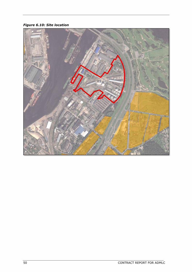
50 CONTRACT REPORT FOR ADMLC
Figure 6.10: Site location
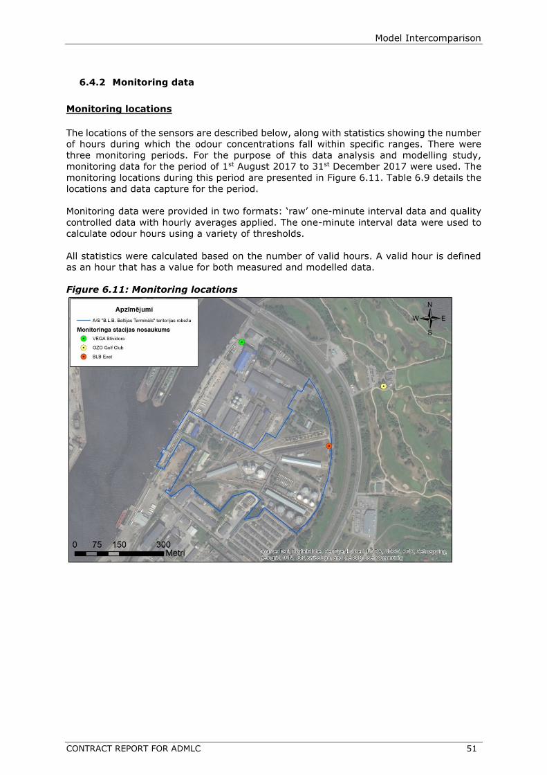
Model Intercomparison
CONTRACT REPORT FOR ADMLC 51
6.4.2 Monitoring data
Monitoring locations
The locations of the sensors are described below, along with statistics showing the number
of hours during which the odour concentrations fall within specific ranges. There were
three monitoring periods. For the purpose of this data analysis and modelling study,
monitoring data for the period of 1st August 2017 to 31st December 2017 were used. The
monitoring locations during this period are presented in Figure 6.11. Table 6.9 details the
locations and data capture for the period.
Monitoring data were provided in two formats: ‘raw’ one-minute interval data and quality
controlled data with hourly averages applied. The one-minute interval data were used to
calculate odour hours using a variety of thresholds.
All statistics were calculated based on the number of valid hours. A valid hour is defined
as an hour that has a value for both measured and modelled data.
Figure 6.11: Monitoring locations

52 CONTRACT REPORT FOR ADMLC
Table 6.9: Monitoring data capture
Monitor Valid hours % capture
BLB East 3445 93.8%
OZO Golf Club 3667 99.9%
VEGA Stividors 2543 69.3%
Monitored values
Odour values were monitored using an Alpha MOS continuous electronic nose (‘e-nose’)
odour monitoring system, or ‘RQ Box’ (Alpha MOS, 2015). The RQ Box was made up of a
photoionization detector (PID) sensor, electrochemical cells and metal oxide
semiconductor (MOS) sensors. Sensor measurements were compared to laboratory
conditions using dynamic olfactometry, and converted to an odour concentration that
correlates with the human sense of smell by means of a mathematical model.
Analysis of monitoring data statistics
The overall mean and the 98th percentile of hourly average concentration values are given
in Table 6.10. Also shown are the results of the odour hour calculations, where an ‘odour
hour’ is defined as an hour that has an odour concentration above a threshold for at least
10% of the time. Odour hours for valid hours were calculated from the monitoring dataset,
for two threshold values, for each of the stations. Note that these thresholds were used
for illustration purposes only, and calculation of odour hours using these values does not
necessarily translate to odour annoyance.
Table 6.10: Monitored mean and 98th percentile odour concentrations and
number of odour hours using two different threshold values
Monitor Mean
(ouE/m3) 98th percentile
(ouE/m3)
5 ouE/m3
threshold
1.5 ouE/m3
threshold
Count % odour
hours Count
% odour hours
BLB East 2.82 7.2 458 13.3 2981 86.5
OZO Golf
Club 1.81 9.7 402 11.0 1562 42.6
VEGA Stividors
4.54 21.0 875 34.4 2191 86.2
Peak-to-mean ratios were also calculated from the measurement dataset. As discussed
further in Section 7.2.2, the peak does not have a standardised definition and is often
defined as a range of percentiles, the maximum or by the application of a standard
deviation relationship. Tables 6.11 to 6.13 show the frequency of values calculated based
on all of the definitions given in Section 7.2.2, giving the range of ratios for each of the
valid monitoring hours. The fluctuation intensity = / Cm.
The range of ratios that occurs most often is 1-2, for all ‘peak’ definitions, and for all
monitoring locations. The baseline of the data appears to be artificially high, with few
records of zero or very low concentrations, and it is possible that this is an artefact of the
methodology, and at least in part responsible for the low peak-to-mean ratios.

Model Intercomparison
CONTRACT REPORT FOR ADMLC 53
Table 6.11: Peak-to-mean ratio frequencies using a range of ‘peak’ definitions
at BLB East monitoring station Peak-to-
mean ratio range
Maximum 99th
percentile 98th
percentile 90th
percentile Fluctuation
intensity
< 1 46 46 63 153 0
1-2 3343 3345 3331 3278 3441
2-3 41 43 42 10 4
3-4 9 6 5 4 0
4-5 3 3 3 0 0
> 5 3 2 1 0 0
Table 6.12: Peak-to-mean ratio frequencies using a range of ‘peak’ definitions
at Ozo Golf Club monitoring station Peak-to-
mean ratio
range
Maximum 99th
percentile 98th
percentile 90th
percentile Fluctuation
intensity
< 1 199 1817 1882 2181 0
1-2 2779 1078 1081 977 3472
2-3 149 371 341 277 121
3-4 64 131 119 102 34
4-5 52 71 75 47 18
> 5 424 199 169 83 22
Table 6.13: Peak-to-mean ratio frequencies using a range of ‘peak’ definitions
at Vega monitoring station Peak-to-
mean ratio range
Maximum 99th
percentile 98th
percentile 90th
percentile Fluctuation
intensity
< 1 19 19 28 61 0
1-2 2330 2354 2363 2447 2539
2-3 155 140 127 34 4
3-4 31 22 19 1 0
4-5 3 4 3 0 0
> 5 5 4 3 0 0
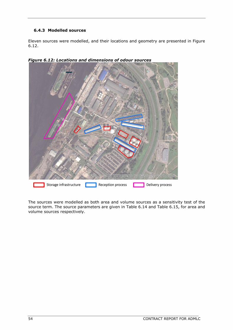
54 CONTRACT REPORT FOR ADMLC
6.4.3 Modelled sources
Eleven sources were modelled, and their locations and geometry are presented in Figure
6.12.
Figure 6.12: Locations and dimensions of odour sources
The sources were modelled as both area and volume sources as a sensitivity test of the
source term. The source parameters are given in Table 6.14 and Table 6.15, for area and
volume sources respectively.
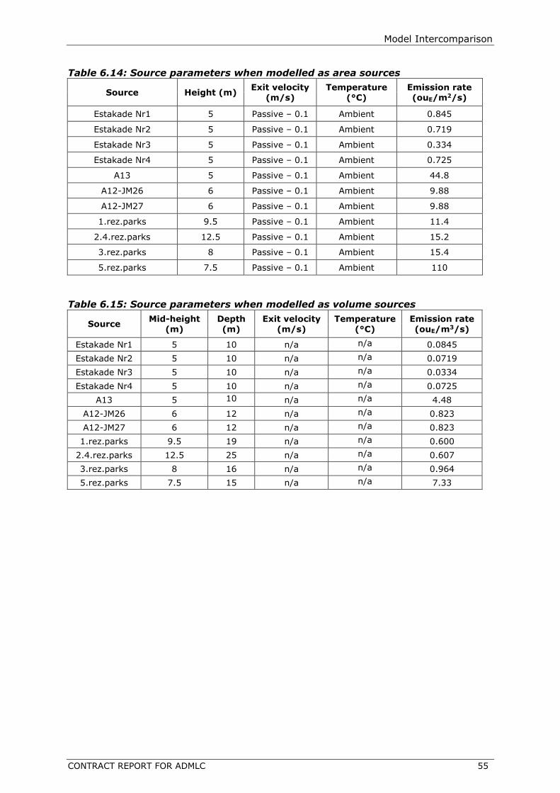
Model Intercomparison
CONTRACT REPORT FOR ADMLC 55
Table 6.14: Source parameters when modelled as area sources
Source Height (m) Exit velocity
(m/s) Temperature
(°C) Emission rate (ouE/m2/s)
Estakade Nr1 5 Passive – 0.1 Ambient 0.845
Estakade Nr2 5 Passive – 0.1 Ambient 0.719
Estakade Nr3 5 Passive – 0.1 Ambient 0.334
Estakade Nr4 5 Passive – 0.1 Ambient 0.725
A13 5 Passive – 0.1 Ambient 44.8
A12-JM26 6 Passive – 0.1 Ambient 9.88
A12-JM27 6 Passive – 0.1 Ambient 9.88
1.rez.parks 9.5 Passive – 0.1 Ambient 11.4
2.4.rez.parks 12.5 Passive – 0.1 Ambient 15.2
3.rez.parks 8 Passive – 0.1 Ambient 15.4
5.rez.parks 7.5 Passive – 0.1 Ambient 110
Table 6.15: Source parameters when modelled as volume sources
Source Mid-height
(m) Depth (m)
Exit velocity (m/s)
Temperature (°C)
Emission rate (ouE/m3/s)
Estakade Nr1 5 10 n/a n/a 0.0845
Estakade Nr2 5 10 n/a n/a 0.0719
Estakade Nr3 5 10 n/a n/a 0.0334
Estakade Nr4 5 10 n/a n/a 0.0725
A13 5 10 n/a n/a 4.48
A12-JM26 6 12 n/a n/a 0.823
A12-JM27 6 12 n/a n/a 0.823
1.rez.parks 9.5 19 n/a n/a 0.600
2.4.rez.parks 12.5 25 n/a n/a 0.607
3.rez.parks 8 16 n/a n/a 0.964
5.rez.parks 7.5 15 n/a n/a 7.33
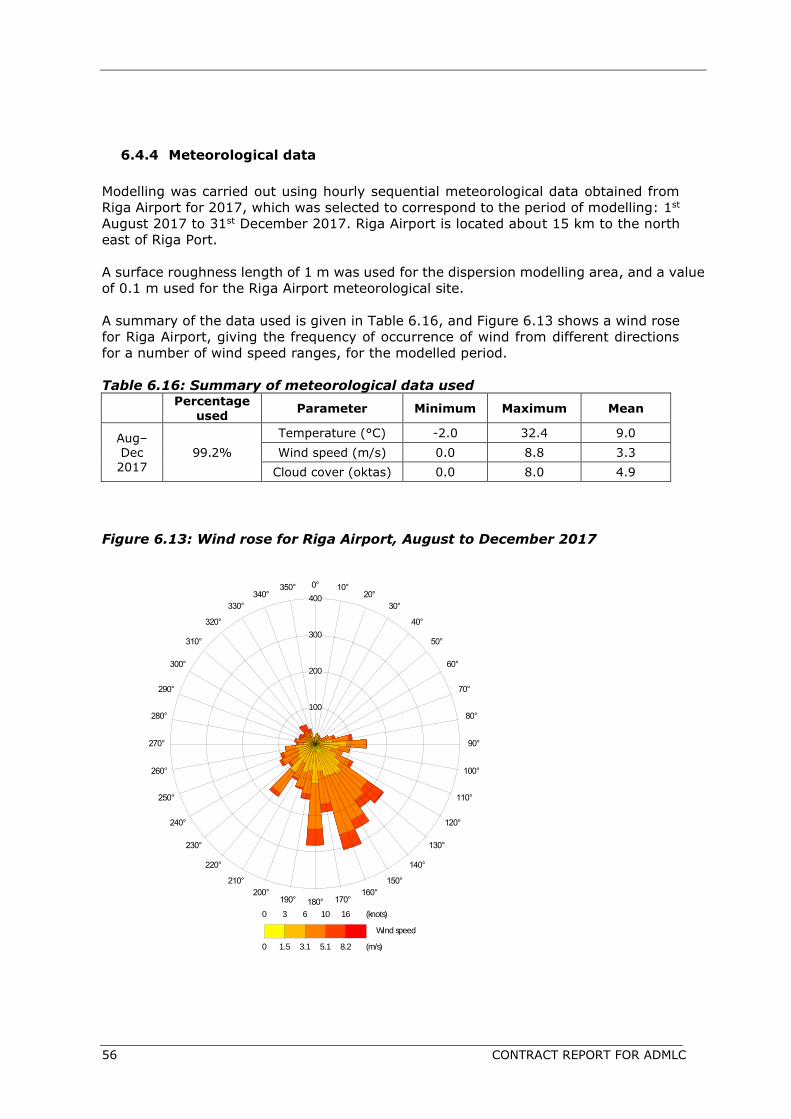
56 CONTRACT REPORT FOR ADMLC
6.4.4 Meteorological data
Modelling was carried out using hourly sequential meteorological data obtained from
Riga Airport for 2017, which was selected to correspond to the period of modelling: 1st
August 2017 to 31st December 2017. Riga Airport is located about 15 km to the north
east of Riga Port.
A surface roughness length of 1 m was used for the dispersion modelling area, and a value
of 0.1 m used for the Riga Airport meteorological site.
A summary of the data used is given in Table 6.16, and Figure 6.13 shows a wind rose
for Riga Airport, giving the frequency of occurrence of wind from different directions
for a number of wind speed ranges, for the modelled period.
Table 6.16: Summary of meteorological data used
Percentage
used Parameter Minimum Maximum Mean
Aug–Dec 2017
99.2%
Temperature (°C) -2.0 32.4 9.0
Wind speed (m/s) 0.0 8.8 3.3
Cloud cover (oktas) 0.0 8.0 4.9
Figure 6.13: Wind rose for Riga Airport, August to December 2017
P:\FM\FM1166_ADMLC_odour\Modelling\Working\ELLE_Dataset\Runs\Met\meteodati-Riga2017.met
0
0
3
1.5
6
3.1
10
5.1
16
8.2
(knots)
(m/s)
Wind speed
0° 10°20°
30°
40°
50°
60°
70°
80°
90°
100°
110°
120°
130°
140°
150°
160°170°180°190°
200°
210°
220°
230°
240°
250°
260°
270°
280°
290°
300°
310°
320°
330°
340°350°
100
200
300
400
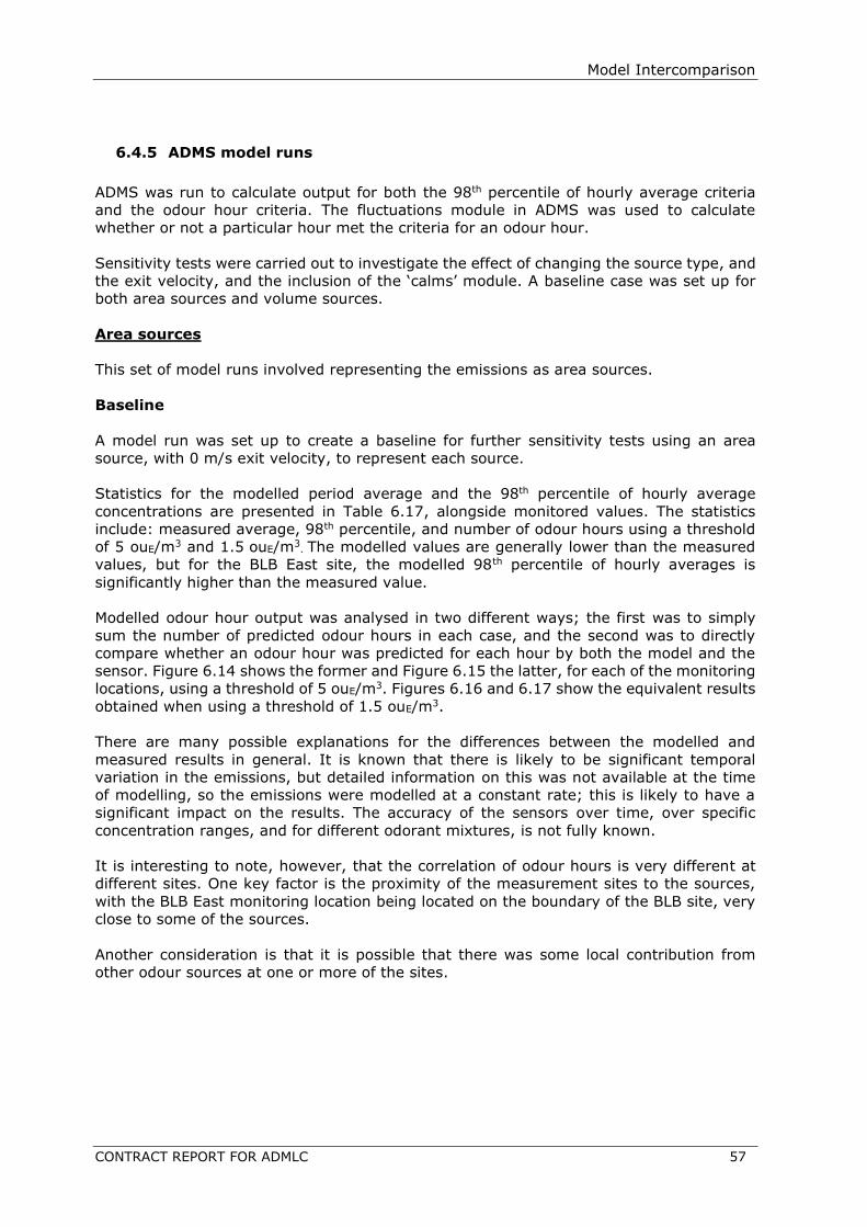
Model Intercomparison
CONTRACT REPORT FOR ADMLC 57
6.4.5 ADMS model runs
ADMS was run to calculate output for both the 98th percentile of hourly average criteria
and the odour hour criteria. The fluctuations module in ADMS was used to calculate
whether or not a particular hour met the criteria for an odour hour.
Sensitivity tests were carried out to investigate the effect of changing the source type, and
the exit velocity, and the inclusion of the ‘calms’ module. A baseline case was set up for
both area sources and volume sources.
Area sources
This set of model runs involved representing the emissions as area sources.
Baseline
A model run was set up to create a baseline for further sensitivity tests using an area
source, with 0 m/s exit velocity, to represent each source.
Statistics for the modelled period average and the 98th percentile of hourly average
concentrations are presented in Table 6.17, alongside monitored values. The statistics
include: measured average, 98th percentile, and number of odour hours using a threshold
of 5 ouE/m3 and 1.5 ouE/m3. The modelled values are generally lower than the measured
values, but for the BLB East site, the modelled 98th percentile of hourly averages is
significantly higher than the measured value.
Modelled odour hour output was analysed in two different ways; the first was to simply
sum the number of predicted odour hours in each case, and the second was to directly
compare whether an odour hour was predicted for each hour by both the model and the
sensor. Figure 6.14 shows the former and Figure 6.15 the latter, for each of the monitoring
locations, using a threshold of 5 ouE/m3. Figures 6.16 and 6.17 show the equivalent results
obtained when using a threshold of 1.5 ouE/m3.
There are many possible explanations for the differences between the modelled and
measured results in general. It is known that there is likely to be significant temporal
variation in the emissions, but detailed information on this was not available at the time
of modelling, so the emissions were modelled at a constant rate; this is likely to have a
significant impact on the results. The accuracy of the sensors over time, over specific
concentration ranges, and for different odorant mixtures, is not fully known.
It is interesting to note, however, that the correlation of odour hours is very different at
different sites. One key factor is the proximity of the measurement sites to the sources,
with the BLB East monitoring location being located on the boundary of the BLB site, very
close to some of the sources.
Another consideration is that it is possible that there was some local contribution from
other odour sources at one or more of the sites.
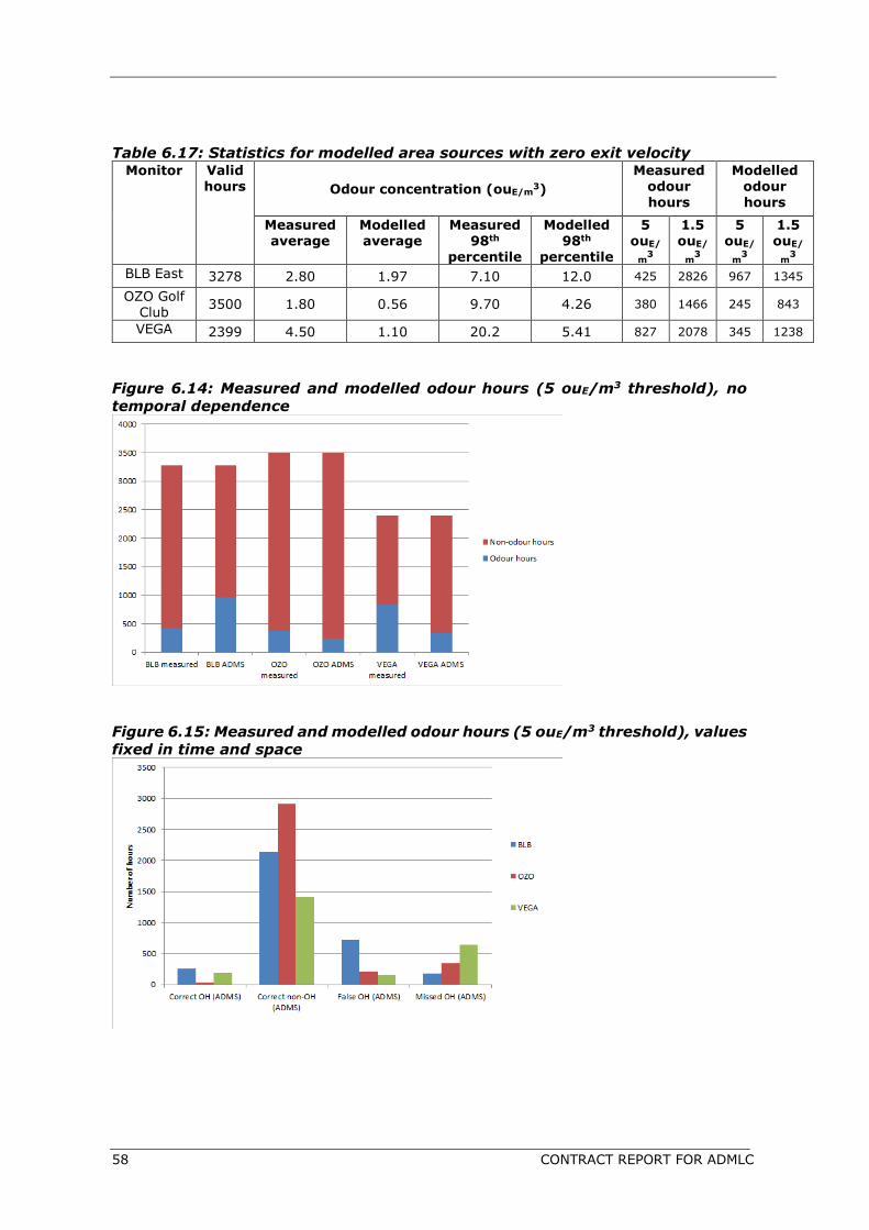
58 CONTRACT REPORT FOR ADMLC
Table 6.17: Statistics for modelled area sources with zero exit velocity Monitor Valid
hours Odour concentration (ouE/m3)
Measured odour hours
Modelled odour hours
Measured average
Modelled average
Measured 98th
percentile
Modelled 98th
percentile
5 ouE/
m3
1.5 ouE/
m3
5 ouE/
m3
1.5 ouE/
m3
BLB East 3278 2.80 1.97 7.10 12.0 425 2826 967 1345
OZO Golf Club
3500 1.80 0.56 9.70 4.26 380 1466 245 843
VEGA 2399 4.50 1.10 20.2 5.41 827 2078 345 1238
Figure 6.14: Measured and modelled odour hours (5 ouE/m3 threshold), no
temporal dependence
Figure 6.15: Measured and modelled odour hours (5 ouE/m3 threshold), values
fixed in time and space
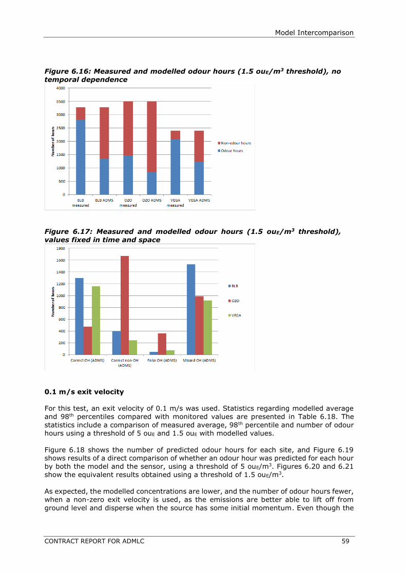
Model Intercomparison
CONTRACT REPORT FOR ADMLC 59
Figure 6.16: Measured and modelled odour hours (1.5 ouE/m3 threshold), no
temporal dependence
Figure 6.17: Measured and modelled odour hours (1.5 ouE/m3 threshold),
values fixed in time and space
0.1 m/s exit velocity
For this test, an exit velocity of 0.1 m/s was used. Statistics regarding modelled average
and 98th percentiles compared with monitored values are presented in Table 6.18. The
statistics include a comparison of measured average, 98th percentile and number of odour
hours using a threshold of 5 ouE and 1.5 ouE with modelled values.
Figure 6.18 shows the number of predicted odour hours for each site, and Figure 6.19
shows results of a direct comparison of whether an odour hour was predicted for each hour
by both the model and the sensor, using a threshold of 5 ouE/m3. Figures 6.20 and 6.21
show the equivalent results obtained using a threshold of 1.5 ouE/m3.
As expected, the modelled concentrations are lower, and the number of odour hours fewer,
when a non-zero exit velocity is used, as the emissions are better able to lift off from
ground level and disperse when the source has some initial momentum. Even though the

60 CONTRACT REPORT FOR ADMLC
exit velocity is still very low, it can be seen that this change has a significant effect on the
modelled statistics.
Table 6.18: Statistics for modelled area sources with an exit velocity of 0.1 m/s
Monitor Valid hours
Odour concentration (ouE/m3)
Measured
odour hours
Modelled
odour hours
Measured average
Modelled average
Measured 98th
percentile
Modelled 98th
percentile
5 ouE/
m3
1.5 ouE/
m3
5 ouE/
m3
1.5 ouE/
m3
BLB East 3278 2.80 1.72 7.10 10.1 425 2826 899 1304
OZO Golf
Club
3500 1.80 0.53 9.70 4.10 380 1466 220 833
VEGA 2399 4.50 1.04 20.2 5.17 827 2078 316 1221
Figure 6.18: Measured and modelled odour hours (5 ouE/m3 threshold), no
temporal dependence
Figure 6.19: Measured and modelled odour hours (5 ouE/m3 threshold), values
fixed in time and space
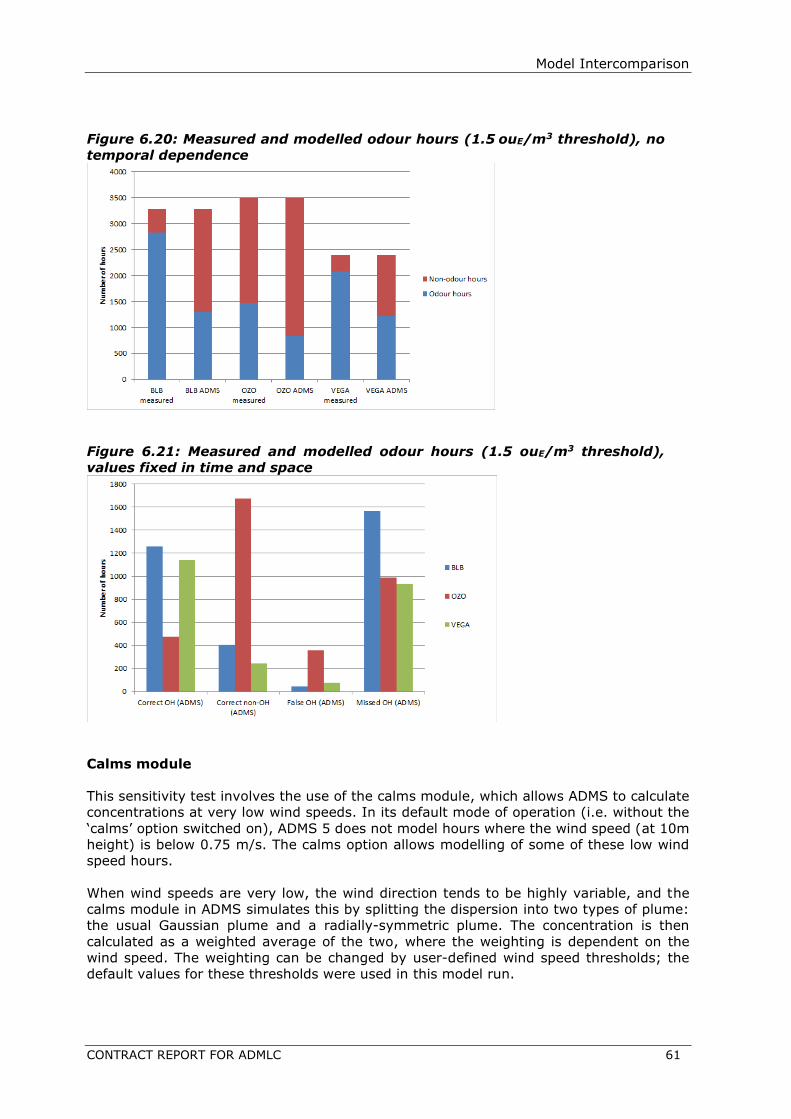
Model Intercomparison
CONTRACT REPORT FOR ADMLC 61
Figure 6.20: Measured and modelled odour hours (1.5 ouE/m3 threshold), no
temporal dependence
Figure 6.21: Measured and modelled odour hours (1.5 ouE/m3 threshold),
values fixed in time and space
Calms module
This sensitivity test involves the use of the calms module, which allows ADMS to calculate
concentrations at very low wind speeds. In its default mode of operation (i.e. without the
‘calms’ option switched on), ADMS 5 does not model hours where the wind speed (at 10m
height) is below 0.75 m/s. The calms option allows modelling of some of these low wind
speed hours.
When wind speeds are very low, the wind direction tends to be highly variable, and the
calms module in ADMS simulates this by splitting the dispersion into two types of plume:
the usual Gaussian plume and a radially-symmetric plume. The concentration is then
calculated as a weighted average of the two, where the weighting is dependent on the
wind speed. The weighting can be changed by user-defined wind speed thresholds; the
default values for these thresholds were used in this model run.

62 CONTRACT REPORT FOR ADMLC
Table 6.19 presents results with the addition of the calms module calculations to the
passive area source baseline run. The fluctuations module cannot be run whilst the calms
module is being used, so odour hour statistics were not generated.
The results show that, in this case, the use of the calms module has slightly increased both
the period average and 98th percentile of hourly averages for all sites, giving slightly closer
agreement at the OZO and VEGA sites, but reducing the agreement at the BLB site.
Table 6.19: Statistics for model run with calms module included
Monitor Valid
hours
Odour concentration (ouE/m3)
Measured Modelled
Average 98th
percentile Average
98th
percentile
BLB East 3421 2.81 7.10 2.25 12.94
OZO Golf
Club 3643 1.80 9.70 0.65 4.98
VEGA 2520 4.47 20.20 1.25 6.15
Volume source
This set of model runs involved representing the emissions as volume sources. A sensitivity
test was carried out in a similar manner as for the area source model runs using the calms
module to see the effects on the concentration statistics. A volume source does not have
an exit velocity associated with it in ADMS, so no sensitivity test of this parameter was
carried out for the volume source modelling.
Baseline
Statistics for modelled and monitored average and 98th percentile concentrations are
presented in Table 6.18. The statistics include: measured average, 98th percentile, and
number of odour hours using a threshold of 5 ouE and 1.5 ouE. The modelled averages were
lower than the measured values. This is also the case for the 98th percentile values, with
the exception of BLB East, which had a higher modelled 98th percentile value.
Figure 6.22 shows the number of predicted odour hours for each site, and Figure 6.20
shows results of a direct comparison of whether an odour hour was predicted for each hour
by both the model and the sensor, using a threshold of 5 ouE/m3. Figures 6.24 and 6.25
show the equivalent results obtained using a threshold of 1.5 ouE/m3. The results show
that changing the source type has only a modest impact on the modelled statistics. This is
as expected for this type of release, with no inherent buoyancy.
Table 6.20: Statistics for the modelled volume sources Monitor Valid
hours Odour concentration (ouE/m
3) Measured
odour hours Modelled
odour hours
Measured average
Modelled average
Measured 98th
percentile
Modelled 98th
percentile
5 ouE/
m3
1.5 ouE/
m3
5 ouE/
m3
1.5 ouE/
m3
BLB East 3278 2.80 2.12 7.10 13.0 425 2826 998 1369
OZO Golf Club
3500 1.80 0.57 9.70 4.42 380 1466 222 844
VEGA 2399 4.50 1.10 20.2 5.33 827 2078 274 1237

Model Intercomparison
CONTRACT REPORT FOR ADMLC 63
Figure 6.22: Measured and modelled odour hours (5 ouE/m3 threshold), no
temporal dependence
Figure 6.23: Measured and modelled odour hours (5 ouE/m3 threshold), values
fixed in time and space

64 CONTRACT REPORT FOR ADMLC
Figure 6.24: Measured and modelled odour hours (1.5 ouE/m3 threshold), no
temporal dependence
Figure 6.25: Measured and modelled odour hours (1.5 ouE/m3 threshold), values
fixed in time and space

Model Intercomparison
CONTRACT REPORT FOR ADMLC 65
Calms module
Table 6.21 presents results with the addition of the calms module calculations to the
volume source baseline run.
The results show that, as previously, the use of the calms module slightly increased both
the period average and 98th percentile of hourly averages for all sites, giving slightly closer
agreement at the OZO and VEGA sites, but reducing the agreement at the BLB site.
Table 6.21: Statistics for model run with calms module included
Monitor
Odour concentration (ouE/m3)
Valid
hours
Measured Modelled
Average 98th
percentile Average 98th percentile
BLB East 3421 2.81 7.10 2.41 14.1
OZO Golf Club
3643 1.80 9.70 0.67 5.09
VEGA 2520 4.47 20.2 1.25 6.05
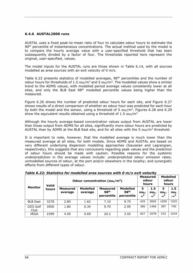
66 CONTRACT REPORT FOR ADMLC
6.4.6 AUSTAL2000 runs
AUSTAL uses a fixed peak-to-mean ratio of four to calculate odour hours to estimate the
90th percentile of instantaneous concentrations. The actual method used by the model is
to compare the hourly average value with a user-specified threshold that has been
subsequently divided by a factor of four. The thresholds reported here represent the
original, user-specified, values.
The model inputs for the AUSTAL runs are those shown in Table 6.14, with all sources
modelled as area sources with an exit velocity of 0 m/s.
Table 6.22 presents statistics of modelled averages, 98th percentiles and the number of
odour hours for thresholds of 1.5 ouE/m3 and 5 ouE/m3. The modelled values show a similar
trend to the ADMS values, with modelled period average values consistently lower at all
sites, and only the BLB East 98th modelled percentile values being higher than the
measured.
Figure 6.26 shows the number of predicted odour hours for each site, and Figure 6.27
shows results of a direct comparison of whether an odour hour was predicted for each hour
by both the model and the sensor, using a threshold of 5 ouE/m3. Figures 6.28 and 6.29
show the equivalent results obtained using a threshold of 1.5 ouE/m3
Although the hourly average-based concentration values output from AUSTAL are lower
than those output from ADMS for all sites, significantly more odour hours are predicted by
AUSTAL than by ADMS at the BLB East site, and for all sites with the 5 ouE/m3 threshold.
It is important to note, however, that the modelled average is much lower than the
measured average at all sites, for both models. Since ADMS and AUSTAL are based on
very different underlying dispersion modelling approaches (Gaussian and Lagrangian,
respectively), this suggests that any conclusions regarding peak values and the prediction
of odour hours should be made with caution. Possible reasons for the systemic
underprediction in the average values include: underpredicted odour emission rates;
unmodelled sources of odour, at the port and/or elsewhere in the locality; and synergistic
effects from different types of odour.
Table 6.22: Statistics for modelled area sources with 0 m/s exit velocity
Monitor Valid hours
Odour concentration (ouE/m3)
Measured
odour
hours
Modelled
odour
hours
Measured average
Modelled average
Measured 98th
percentile
Modelled 98th
percentile
5 ouE/
m3
1.5 ouE/
m3
5 ouE/
m3
1.5 ouE
/m3
BLB East 3278 2.80 1.62 7.10 9.75 425 2826 1059 1525
OZO Golf Club
3500 1.80 0.34 9.70 2.95 380 1466 387 740
VEGA 2399 4.50 0.69 20.2 3.55 827 2078 533 1034
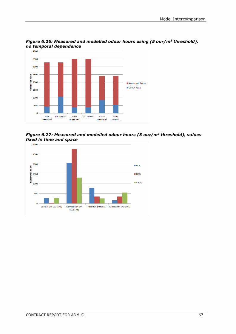
Model Intercomparison
CONTRACT REPORT FOR ADMLC 67
Figure 6.26: Measured and modelled odour hours using (5 ouE/m3 threshold),
no temporal dependence
Figure 6.27: Measured and modelled odour hours (5 ouE/m3 threshold), values
fixed in time and space

68 CONTRACT REPORT FOR ADMLC
Figure 6.28: Measured and modelled odour hours (1.5 ouE/m3 threshold), no
temporal dependence
Figure 6.29: Measured and modelled odour hours (1.5 ouE/m3 threshold), values
fixed in time and space
Model Intercomparison
CONTRACT REPORT FOR ADMLC 69
6.5 Styria pig farm dataset
Oettl et al (2018a) describe field inspections carried out at a pig farm in Styria, Austria,
including odour assessment. A dataset of the field inspections and associated model setup
information was provided for this model intercomparison exercise by the lead author of the
article.
6.5.1 Experimental setup and dataset
The inspections were carried out between the 1st of February and the 31st of July, 2017,
in accordance with the EN 16841-1 European Standard, with in-situ odour measurements
carried out by suitably qualified panel members. Each field inspection measurement
comprised a 10-minute sniffing time, and if at least 10 odour detections were experienced
by the panel member during that time, then the period was classed as an 'odour hour'.
An average of 1225 pigs were housed in a shed, and odour emissions from the shed were
vented from six stacks, each with a diameter of 0.8 m. There was also an open manure
storage tank tank adjacent to the shed, with a diameter of 17 m.
The nearest of the twelve measurement points was located less than 10 m from the shed,
and the furthest 300 m away. The points were mainly to the north east and south west of
the shed, reflecting the prevailing local wind directions. A total of 52 measurements were
carried out, at each of the measurement points, and were evenly spread over all days of
the week and over 24 hours of the day.
The terrain of the site and surrounding area was generally flat and comprised mainly
farmland.
The final outcome from the field inspection was an odour hour frequency for each of the
twelve measurement points over the whole period, expressed as a percentage.
The authors also carried out odour dispersion modelling, using GRAL, applying two different
methods to calculate the peak (90th percentile) concentrations from hourly average
concentrations: the first was a fixed peak-to-mean factor of 4, and the second was a
concentration-variance model, as described in Section 7.2.3. A value of 1 ou/m3 was used
as the threshold to trigger an odour hour in the modelling.
The locations of the sources, measurement points and buildings are given in Figure 6.30,
where the vertical bars show the 95% confidence interval of the field observations. The
results from the field inspection and GRAL modelling are given in Figure 6.31 (both figures
are reproduced from the Oettl et al (2018a) article).
As shown in Figure 6.30, the odour measurement sites are labelled numerically in
approximate order of increasing distance from the odour sources.
The dataset provided for the current work included the GRAL model input files with details
of the model input parameters and setup. Meteorological data from an on-site sonic
anemometer, measured at a height of 7 m, was also provided, covering the whole
experimental period; the data comprised hourly values for the wind speed and direction,
and the atmospheric stability.

70 CONTRACT REPORT FOR ADMLC
Figure 6.30: Aerial image of experiment site, showing sources and
measurement points 1 to 12.
Figure 6.31: Results from field measurements and GRAL modelling

Model Intercomparison
CONTRACT REPORT FOR ADMLC 71
6.5.2 Model runs
Model setup and inputs
Model runs for the current study were carried out using ADMS and AERMOD, using the
meteorological data provided with the dataset, comprising hourly sequential data over the
whole experiment period (1st of February to the 31st of July). Two scenarios were
modelled: one including building effects, and another without building effects. This was
primarily because the fluctuations module in ADMS cannot be run with building effects, but
it also allowed additional information to be obtained regarding the treatment of buildings
in both models, and how this influences modelled concentrations over different distances.
Table 6.23 shows the modelled source parameters. Note that the values for stacks 1 to 6
represent those for a single stack; all stacks had the same values. The circular geometry
of the manure storage area was approximated by a complex polygon area source. The
emission rate for each stack was 3764 ouE/s, and the emission rate for the manure storage
source was 7 ouE/m2/s.
Table 6.23: Modelled source parameters
Name Source
type
Height
(m)
Diameter
(m)
Area
(m2)
Exit
Velocity
(m/s)
Exit
temperature
(°C)
Stacks 1 to 6 Point 8.5 0.75 - 5
15 Manure
storage Area 4 - 232 0.02
Figure 6.31 shows a wind rose for the modelled period. No complex terrain effects were
included; the modelled surface roughness length was 0.1 m in each case.
Figure 6.31: Wind rose for 1st February to 31st July 2017
0
0
3
1.5
6
3.1
10
5.1
16
8.2
(knots)
(m/s)
Wind speed
0° 10°20°
30°
40°
50°
60°
70°
80°
90°
100°
110°
120°
130°
140°
150°
160°170°180°190°
200°
210°
220°
230°
240°
250°
260°
270°
280°
290°
300°
310°
320°
330°
340°350°
100
200
300
400
72 CONTRACT REPORT FOR ADMLC
For both models, and both scenarios, a fixed peak-to-mean value was used to calculate
the peak (the 90th percentile) from the hourly averages. For the ‘without buildings’
scenario, in ADMS, the fluctuations module was also used, and the newly-developed ‘odour
hour’ functionality was used to determine whether each hour was an odour hour, based on
an input averaging time of 10 s. For all odour hour calculations, a value of 1 ou/m3 was
used as the threshold to trigger an odour hour, as in the GRAL modelling.
Results
Figures 6.32 and 6.33 show the results for the ADMS modelling, with and without building
effects, respectively. Figures 6.34 and 6.35 show corresponding results for the AERMOD
modelling.
For the ADMS results, for both the ‘with building’ and ‘without building’ scenarios, the fixed
peak-to-mean and fluctuations module results show good agreement with the field
inspection measurements for receptors 6 to 12. These receptors represent distances of
around 100 to 300 m from the sources. Receptor 1 is very close to the sources and building,
and, as expected, there is substantial underprediction for the ‘without building’ scenario,
due to the high building cavity concentrations not being modelled in this scenario, although
there is also some underprediction for the ‘with building’ scenario.
For the AERMOD results, for both the ‘with building’ and ‘without building’ scenarios there
was very good agreement for some receptors, and a tendency to overpredict for the
remainder. The exception to this was the expected substantial underprediction for
Receptor 1 in the ‘without building’ scenario in AERMOD, due to the high concentrations
within the building cavity not being modelled in this scenario. Oettl et al (2018a) found
that there were high measured odour hour frequencies very close to the source, suggesting
that building effects were significant. As described above, this is reflected in both the ADMS
and AERMOD ‘without building’ results.
It is interesting that, for the ADMS results in particular, the application of the fixed peak-
to-mean value of four does not lead to the general overprediction that was seen in the
equivalent GRAL results. For the ADMS results, there is underprediction in the near-field,
and good agreement in the far-field with a slight tendency to underpredict. The results
from the ADMS fluctuation module are similar to those given by the fixed peak-to-mean
calculation in this case, with the fixed peak-to-mean results being slightly higher. For the
AERMOD results, the general overprediction is modest, with the exception of Receptor 1
for the ‘with building’ scenario.

Model Intercomparison
CONTRACT REPORT FOR ADMLC 73
Figure 6.32: ADMS results for the ‘with building’ scenario
Figure 6.33: ADMS results for the ‘without building’ scenario

74 CONTRACT REPORT FOR ADMLC
Figure 6.34: AERMOD results for the ‘with building’ scenario
Figure 6.35: AERMOD results for the ‘without building’ scenario
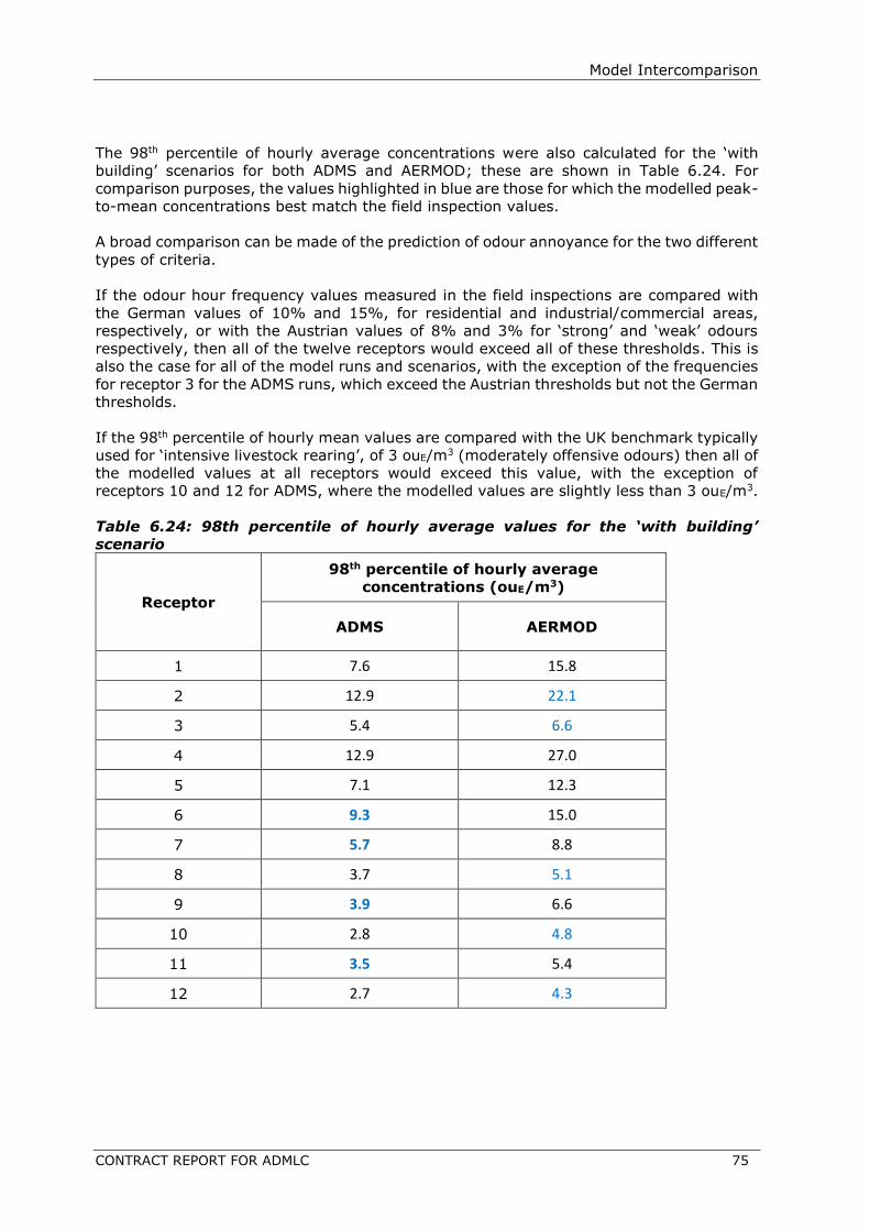
Model Intercomparison
CONTRACT REPORT FOR ADMLC 75
The 98th percentile of hourly average concentrations were also calculated for the ‘with
building’ scenarios for both ADMS and AERMOD; these are shown in Table 6.24. For
comparison purposes, the values highlighted in blue are those for which the modelled peak-
to-mean concentrations best match the field inspection values.
A broad comparison can be made of the prediction of odour annoyance for the two different
types of criteria.
If the odour hour frequency values measured in the field inspections are compared with
the German values of 10% and 15%, for residential and industrial/commercial areas,
respectively, or with the Austrian values of 8% and 3% for ‘strong’ and ‘weak’ odours
respectively, then all of the twelve receptors would exceed all of these thresholds. This is
also the case for all of the model runs and scenarios, with the exception of the frequencies
for receptor 3 for the ADMS runs, which exceed the Austrian thresholds but not the German
thresholds.
If the 98th percentile of hourly mean values are compared with the UK benchmark typically
used for ‘intensive livestock rearing’, of 3 ouE/m3 (moderately offensive odours) then all of
the modelled values at all receptors would exceed this value, with the exception of
receptors 10 and 12 for ADMS, where the modelled values are slightly less than 3 ouE/m3.
Table 6.24: 98th percentile of hourly average values for the ‘with building’
scenario
Receptor
98th percentile of hourly average
concentrations (ouE/m3)
ADMS AERMOD
1 7.6 15.8
2 12.9 22.1
3 5.4 6.6
4 12.9 27.0
5 7.1 12.3
6 9.3 15.0
7 5.7 8.8
8 3.7 5.1
9 3.9 6.6
10 2.8 4.8
11 3.5 5.4
12 2.7 4.3
76 CONTRACT REPORT FOR ADMLC
6.6 Summary
These model data comparisons have given insight into the extent to which different models
and approaches are able to replicate metrics relevant to odour prediction, but drawing firm
conclusions regarding the capabilities of the different models and the methodologies is not
straightforward in view of the wide differences in the models’ features and approach. For
this reason, the modelling exercises can be considered as case studies, enabling the
illustration and exploration of some of the issues discussed elsewhere in this report.
In the Riga Port dataset, complex source types and highly temporal emission patterns, as
well as potential interference from other sources of odour, are key challenges in the odour
dispersion modelling. Differences between modelled and measured statistics will be, to
some degree, due to these factors, and it is difficult to differentiate between these and
other aspects of the modelling. Despite these challenges, this is an evolving project, and
the modelling and results from this provide an opportunity to consider realistic high-
resolution odour measurements and provide an insight into future possibilities for
dispersion model validation using electronic nose technology.
The remaining datasets involve simple and well-characterised sources, and a relatively
straightforward setup in terms of building, terrain and other key effects, all comprising a
single elevated stack within a relatively simple building arrangement and non-complex
terrain. The key challenge of capturing the properties of the high-resolution temporal
measurements, and the associated peak statistics, is therefore more straightforward to
assess.
A clear conclusion from these modelling results is that improved model performance is
achieved for models that can simultaneously consider both building effects and sub-hourly
concentrations, as illustrated by the GRAL results presented by Oettl et al (2018a) for the
Styria pig farm dataset. ADMS can consider both these effects but not simultaneously; the
ADMS model comparisons using the concentration fluctuation module for the OROD and
CEDVAL datasets show that the form of percentile distributions is generally well
represented, but concentrations values in the near field are in some cases underestimated,
probably because of the lack of consideration building effects for these runs. The extent to
which a model with this joint capability outperforms models using peak to mean ratios, as
required by AERMOD and AUSTAL, would require comparisons of these different
approaches using the same base model (e.g. a modified version of ADMS).
Efficacy of the different approaches in odour dispersion modelling
CONTRACT REPORT FOR ADMLC 77
7 EFFICACY OF THE DIFFERENT APPROACHES IN ODOUR DISPERSION MODELLING
As described previously, there are essentially two main types of odour criteria, and hence
two main approaches to regulatory odour dispersion modelling; one approach directly uses
hourly-averaged concentration output, and the other aims to account for sub-hourly
fluctuations in concentrations. This section will discuss the various methods used, and
address the issue of how well they have been demonstrated to identify and predict odour
impacts.
7.1 Percentile of hourly averages approaches
The first of these approaches, calculating the percentile of hourly averages, is relatively
straightforward, in terms of discussing the modelling techniques involved, as this is the
standard mode of operation for most regulatory dispersion models. Air quality criteria,
ambient pollutant measurements and meteorological data are all commonly based on a
one-hour averaging time, and dispersion models have been developed alongside this
framework.
As discussed in Section 2.3, a common criticism of the percentile of hourly averages
approach is that it does not directly take into account the brief periods of high
concentrations that can be experienced as a variable on/off signal, potentially overcoming
olfactory fatigue and causing annoyance. It has been argued, however (e.g. Environment
Agency, 2007b) that the fluctuations are inherently taken into account by the community
response data on which the approach is based, as described in Section 7.1.1.
There are very few formal studies that specifically address the efficacy and reliability of the
metric. Nevertheless, it has been part of standard practice for odour assessment in several
countries, for many years.
This section will use those studies that are available to discuss the reliability of the criteria
in the context of the dispersion modelling used to calculate it, discuss the extent to which
it is a good predictor of nuisance, and investigate the circumstances in which it has been
shown to perform well and those in which it is less reliable.
7.1.1 The origin of the criteria
The development of the odour criteria based on the 98th percentile of hourly averages has
been discussed in detail in several publications (e.g. Bull et al (2014), Brancher et al
(2017), Environmental Protection Agency (2001), Bull and Fromant (2014), Environment
Agency, 2002), so only a brief overview is given here.
Guidelines in the Netherlands have included percentiles of hourly average concentrations
since the mid-1980s. Work carried out in the Netherlands, in 1988, described by Miedema
et al (2000) investigated exposure-annoyance relationships for three different types of
odour source, by means of an interview process and dispersion modelling. This research
found a relationship between the percentage of the population annoyed and the 98th
percentile of hourly average odour concentrations. They found that around 10% of those
interviewed were annoyed when the 98th percentile of hourly average odour
concentrations was 5 ou/m3. Further work carried out in 2000 and 2001, again in the

78 CONTRACT REPORT FOR ADMLC
Netherlands (Miedema et al, 2000) further investigated the exposure-annoyance
relationships using the Long-Term Frequency Distribution Model (LTFDM) as the dispersion
model to calculate the 98th percentile of hourly average concentrations.
A major formal application of the 98th percentile of hourly averages criteria was part of a
UK Public Inquiry for a wastewater treatment plant planning application, in 1993, where a
report from the Netherlands was cited as the source of this metric. A threshold of 5 ou/m3
was used. This, along with the dose-response work summarized above, led to the
development of odour criteria in the UK and in Ireland that applied different thresholds to
different situations, based on the 98th percentile of hourly average odour concentrations
(Bull et al, 2014; Bull and Fromant, 2014).
7.1.2 Challenges for validation
One inherent challenge for dispersion model validation studies involving the 98th percentile
of hourly averages is that this metric cannot practically be calculated by traditional field
measurement campaigns, as measuring concentrations for every hour of the year has been
impractical. It is therefore unsurprising that there is little research that directly tests the
effectiveness of dispersion modelling for this metric. The only real option, historically, has
been comparison studies using complaint records, questionnaires, and similar information,
rather than the more traditional model verification datasets, and, even here there are few
published studies. Those that have been carried out include the work by Sironi et al
(2010), Drew et al (2007), and Bull and Fromont (2014), as described in Section 5.2.
Many authors have identified that the use of complaints records and other community-
based information in model validation needs to be approached with caution (e.g.
Environment Agency, 2002). There are many reasons for this, but, for complaint records
in particular, it is recognised that complaints do not necessarily correspond to
nuisance/annoyance. This can work both ways, as people can experience odour annoyance
and not make complaints, and sometimes it is clear that people lodge complaints in the
absence of annoyance. The latter is discussed by Bull and Fromant (2014), as summarised
in Section 5.2.
Dispersion models have, of course, been validated for many applications other than odour,
including impacts on human health and habitats, so there is a potential wealth of
information that could be mined; though it is important to bear in mind that some odour
sources, such as standard waste water treatment sources, are modelled exclusively for
reasons of odour impact. In addition, the previously mentioned constraint remains, in that
a percentile statistic over a year requires specific data to be measured over a long period
of time. Many validation studies are of much shorter duration, and many that are longer
are based on annual averages or similar. Some air quality standards for the protection of
human health employ high percentile values, and there is potential to use information from
the many validation studies that are based on these standards. Many of these validation
studies, however, involve road traffic sources, rather than source types applicable to odour
modelling.
Advances in field measurement techniques have increasingly facilitated continuous hourly
ambient concentration measurements of odour, and this will hopefully yield many more
datasets for model comparison, as the technology advances and becomes more widely
used. This should enable more validation studies that can incorporate the challenging
aspects of the input data and dispersion modelling as identified, such as temporally varying
emissions, fugitive emissions and low wind speed conditions, and therefore help to fill
knowledge gaps. Until good, robust, relevant datasets are available, assessing the
effectiveness of the 98th percentile of hourly average criteria will remain difficult.
Efficacy of the different approaches in odour dispersion modelling
CONTRACT REPORT FOR ADMLC 79
7.1.3 Trends and reasons for poor prediction in validation studies
The small number of robust validation datasets and studies makes it difficult to draw out
any clear trends. Where model validation studies have been carried out, however, there is
often a theme of underprediction. Several of the validation studies described in Section
5.2, were carried out with the aim of evaluating the 98th percentile of hourly averages.
Bull and Fromont (2014) found that they underestimated the area of odour annoyance in
their modelling study of fifteen wastewater treatment plants, compared with complaint
records. As described in Section 5.2, these discrepancies may have been caused by local
campaigning and/or may have been at least partly explained by the ‘typical’ odour
emissions used, which were estimated from aerial images and, by necessity, did not allow
site-specific circumstances to be taken into account. It is also relevant that there can be
other, unquantified, emissions arising from wastewater works sources, such as
inadequately controlled odour from malfunctioning odour abatement systems.
Sironi et al (2010) multiplied the hourly mean by a factor of 2.3 before calculating the 98th
percentile, and this gave good correlation with their odour questionnaire results. Drew et
al (2007), also with the aim of testing the 98th percentile of hourly averages, found that
they could get better agreement by decreasing the averaging time in the model to less
than an hour; in this model, ADMS, decreasing the averaging time acts to increase the
modelled concentrations. The authors of both of these studies essentially increased the
hourly-averaged concentrations before calculating the 98th percentile, even though they
used different methods to do so. This represents an underprediction of the odour
annoyance on the basis of the 98th percentile of hourly average criteria.
The studies include different modelling approaches (Sironi et al used CALPUFF, and Bull et
al and Drew et al used ADMS) and cover a range of different types of odour sources: animal
rendering sources, landfill sources and wastewater treatment sources.
There are many possible reasons for the underprediction of the reported odour impact.
This could be related to issues with the complaints record, or several other factors; it is
interesting to note that the authors of all three studies express concerns relating to the
modelled emissions, including the inclusion of fugitive emissions, the accuracy of emission
rates, and the lack of temporal variation in the modelled emission rates.
The availability of accurate emission rates for input to dispersion modelling is often cited
as a major challenge. While this is a universal issue that affects all odour criteria (and
hence is discussed further in Section 7.3), it is often implicated as a major, and perhaps
the most important, reason for a lack of agreement between the 98th percentile of hourly
averages from dispersion modelling and odour annoyance (Sniffer, 2014; Environment
Agency, 2007b). Perhaps it should not be surprising that this is the case; since the criteria
are based on a high percentile value, the results, and therefore any decisions, are highly
dependent on a small number of hours per year, and hence temporal variations in
emissions are inherently important. An important consideration for odour emission rates
is, therefore, to what extent they are a ‘snapshot’, and how representative such data can
be. The temporal variability of emission rates is a major discussion point in odour
dispersion modelling.
As described in Section 5.2, Bull and Fromant (2014) identified the use of constant
emission rates, calculated from published ‘typical’ emission factors, as one of the key likely
reasons for discrepancies between their modelled results and the complaints record, for
the simple reason that odour complaints are likely to occur when odour emission rates are
80 CONTRACT REPORT FOR ADMLC
atypical. This seems likely as it is understood that a number of the works considered in the
study had achieved a degree of notoriety through significant odour complaint episodes,
and that was why there was availability of complaints data. In cases where such complaint
episodes were caused by relatively short term plant problems, then the ‘typical’ emission
data used in the study may well not reflect the emission rates that caused the complaint
episodes.
For the modelling study by Drew et al (2007), it is of note that, although they carried out
site-specific measurements to determine odour emissions, they found that their measured
values were much lower than other published values for similar (landfill) sources. They
noted that there was little putrescible material on the surface in the areas that were
selected at random for the measurements, describing the odour emission measurements
as representing a ‘best case scenario’. To reflect the published emission rates, they had to
multiply their measurements by a factor of 10 before using them in their dispersion
modelling. This highlights the significant challenges and uncertainty in the quantification
of odour emissions.
Emission rates are also likely to be a key issue in the Riga port dataset model validation
exercise carried out as part of this project, as described in Section 6.5. A constant emission
rate was used, and it is known that the odour emissions for the port are temporally
variable, depending on the activities being carried out, as well as other factors. Work to
understand this variation is ongoing.
Many dispersion models allow temporal variation of emissions, and modelling such
variations is standard practice for many other applications such as road source modelling
and certain industrial applications, but there is a distinct lack of collated and easily
accessible model input data available for odour emissions. An important factor is the
timescale over which emissions vary; if the variation is mainly seasonal, then this may be
easier to quantify.
Another factor that is often implicated in the efficacy of dispersion modelling in predicting
the 98th percentile of hourly average criteria is meteorology. As mentioned above, the
results, and therefore any decisions, are highly dependent on a small number of hours per
year. Therefore, this means that a small number of meteorological conditions can be
inordinately important, and outcomes can be dominated by certain stabilities, wind
directions, etc. and can be skewed in different directions. These conditions are often not
the prevailing, or even typical, conditions at a given site. Criteria based on low percentile
values, however, lead to results and decisions that are affected by a wider range of
meteorological conditions (Schauberger and Piringer, 2015).
Two of the important factors already discussed in this section are often highly dependent
on the weather: the variation of odour emission rates with different ambient conditions,
and the variation of human receptor behaviour such as spending time in gardens and
opening windows. Atmospheric dispersion is, of course, also inherently affected by
meteorological conditions. Considering these three factors alone covers all three major
components of exposure: the source, pathway and receptor.
There might be particular situations in which all three of the above weather-related factors
act together to exacerbate the odour impact, and other situations in which they mitigate
one another to some extent. If so, it might be that some situations are better and others
worse for cumulative detrimental meteorological effects driving odour annoyance.
If we start with the assumption that expectations of amenity, home ventilation, and other
drivers for annoyance and complaints are likely to be greater during warm, sunny
conditions, then it follows that operations that have higher emissions in these same
Efficacy of the different approaches in odour dispersion modelling
CONTRACT REPORT FOR ADMLC 81
weather conditions and/or have sources that lead to unfavourable dispersion in these
conditions, are likely to generate more odour annoyance and complaints (e.g. Schauberger
et al, 2001).
Early dose-response studies looked at a range of sources. But if the dispersion models did
not have any time-varying emissions included for any of these sources, and if the
annoyance in those studies was not related to weather-dependent human behaviour
factors, then it might be that the 98th percentile of hourly averages is a good indicator of
odour annoyance only for those situations in which atmospheric dispersion is the only
weather-dependent factor.
Sattler and Devanathan (2007) explored the issue of the effect of meteorology on odour
annoyance. The odour impact was estimated based on several different metrics. They
modelled an area source at a wastewater treatment plant with ISCST3 and AERMOD, and
found that they predicted greater odour impacts in winter months than in the summer
months, when emissions were modelled at a constant rate throughout the year. The results
suggested that the impact of such sources, based on dispersion considerations alone,
would be greater during winter. When they added in temporally varying emissions,
however, with higher emissions for higher ambient temperatures, they conversely found
that the overall impact of the sources was greater during summer.
Further understanding of these temporal relationships between emissions and dispersion
could lead to the adoption of alternative approaches that avoid replicating the complex
temporal variation in emissions. This challenge is not unique to odour modelling, and other
dispersion modelling applications have established ways of modelling without the use of
time-varying emission rates. For air quality modelling of short-term, high percentile
criteria, for example, constant ‘peak’ emission rates are often used. For many sources,
these scenarios represent a conservative approach, often used as a screening step, since
emission rates are often independent of meteorological effects. If it can be shown that a
particular odour source is likely to have highest emissions during meteorological conditions
that give unfavourable dispersion, then this could suggest that constant peak emission
rates should be used for dispersion modelling.
One area in which there has been much attention on short-term emissions and criteria in
recent years is the on-demand electricity generation sector, including Short Term
Operating Reserves (STOR). Modelling guidance has included the recommendation of
statistical approaches such as the hypergeometric probability distribution and Monte Carlo
simulations, and it is possible that there may be some scope for lessons learnt in this area
to be applied to odour modelling assessments (Environment Agency and Natural Resources
Wales, 2019).
7.1.4 Possible modifications using variable percentile values
Griffiths (2014) identified “significant shortcomings in traditional single percentile odour
criteria”, in relating the combined effects of frequency and intensity of odours to odour
annoyance, and suggested that a multi-percentile criterion approach is preferable. This
research looked at conceptual ‘models of annoyance’, specifically examining the frequency
and intensity aspects.
One of their models, ‘AM3’, was one in which both the intensity of odour and frequency of
odour events affect the amount of annoyance; this was a conceptual model which fits with
observations and with the FIDOL system. The other models were ‘AM1’, and ‘AM2’. For
‘AM1’, the frequency of odour events affects the level of annoyance but the intensity/
concentration of odour of the events does not. This model fits with the ‘odour hour’ criteria,

82 CONTRACT REPORT FOR ADMLC
where a ‘yes/no’ question of exceeding the threshold for the odour hour is the only way in
which the odour intensity is taken into consideration. For ‘AM2’, the intensity of odour
affects the amount of annoyance, but the frequency of odour events does not.
Analysis of the ‘AM3’ model demonstrated how odour annoyance may result from
concentrations of odour events at more than one percentile level. It was demonstrated
that annoyance could be due to exposure to few events of high odour concentration
(termed ‘acute exposure’), or exposure to many events of low odour concentrations
(‘chronic exposure’), or combinations of these two situations.
A main conclusion of the work was that the typical situation of a single percentile odour
criteria for a receptor of particular sensitivity is unlikely to effectively identify the extent of
odour impact when applied to different environmental situations; in particular, in
environments where the odour concentration distribution patterns are significantly
different to the distributions used to originally develop the criteria. The meteorology,
multiple sources, source configurations and emission profiles were highlighted as being
contenders for giving rise to such differences by environment.
Griffiths goes on to discuss the idea that using a single percentile for odour impact criteria
has the effect of limiting the meteorological conditions that would affect the physical extent
of the odour nuisance impact; the example is given of ground-level sources, where high
percentile criteria lead to the odour impact extent being dominated by stable conditions
with low wind speeds, as opposed to low percentile criteria, where neutral and unstable
conditions are instead important.
He points out that even criteria based on carefully selected multi-percentile values still
might not be able to identify annoyance from the additive effects of acute and chronic
exposure conditions. He goes on to conclude that problems with single-percentile criteria,
also highlighted by other researchers, do not appear to have been a major consideration
for regulators. He suggests that this is an important consideration in the future
development of more effective and harmonised odour criteria.
Brancher et al (2017), in their review of worldwide odour criteria, also include the
recommendation of the development of multi-percentile criteria as one of their major
findings: “A well designed and calibrated multi-percentile criterion framework should in
principle have better skill in predicting odour nuisance incurred by both acute and chronic
odour exposure conditions and variations of these conditions”. They point out the relevance
of risk matrices employed by Victoria, Australia and Norway, which involve a multi-
percentile approach to identify distinct zones of varying risk.
The adoption of multi-percentile criteria is an appealing possibility, because this would be
an easily applied change for many countries and jurisdictions that currently adopt a single-
percentile approach, as it does not involve a fundamental change in modelling
methodology. But there are important considerations to be made when choosing values. A
report by the UK Environment Agency (2002) describes how both ‘fundamental’ and
‘practical’ elements should be considered in selecting a suitable percentile value. As an
example of a fundamental consideration, they cite the fact that a small number of hours
with high concentrations determine whether annoyance occurs, and, as an example of a
practical consideration, the fact that there is an increase in the uncertainty of model results
when predicting very high percentile values, due to the small number of hours involved. It
describes the 98th percentile as a ‘compromise’ between these.

Efficacy of the different approaches in odour dispersion modelling
CONTRACT REPORT FOR ADMLC 83
7.2 Sub-hourly average approaches
The second approach to odour modelling, in which sub-hourly concentrations are
calculated, is covered in this section. The key concepts have been introduced in Section 2,
and are further discussed and explored here.
There are many different approaches for modelling concentration fluctuations. Although
there are complex models and methods, such as computational fluid dynamics (CFD) (e.g.
Hong et al, 2010) and Lagrangian models (e.g. Ferrero et al, 2020) used for the calculation
of high frequency concentrations, these are not widely used in an operational, regulatory
context, and therefore a detailed analysis of these is beyond the scope of this project.
Detailed discussions of these techniques, and the reasons why they have not been adopted
for operational purposes are given by Cassiani et al (2020).
The methods used in modelling fluctuations of odour concentrations for regulatory
purposes are largely empirical in nature. Therefore, when considering model validation and
applicability for calculating sub-hourly average criteria, it is essentially the applicability of
the method used to determine the peak concentration that is being tested; that is the
peak-to-mean ratio, statistical method, etc., rather than the model or model setup. The
uncertainty in these peak-to-mean estimations will, at least, tend to mask any
shortcomings in the model setup.
The different method of calculating peak concentrations will therefore be described in this
section. As introduced in Section 2, there is a hierarchy of approaches for calculating sub-
hourly odour concentrations for regulatory purposes, ranging from a simple application of
a single peak-to-mean ratio, to more sophisticated statistical approaches.
7.2.1 Real world – what affects peak concentrations and fluctuations?
It has long been accepted in regulatory understanding of odour modelling that fluctuating
concentrations are important, and also that the nature of these fluctuations can be highly
variable, depending on the situation.
As described in Section 2.4, the dispersion of a plume can be artificially yet usefully
separated into whole-plume transport and smaller-scale effects, depending on the spatial
scale of the turbulent eddies with respect to the size of the plume. Distinguishing between
these two behaviours can be helpful in understanding the variation in peak-to-mean ratios
in different situations.
Plume behaviour, including meandering, the size of the plume, and turbulent mixing, is
very important in determining fluctuations, and it follows that any factor that can
significantly affect plume behaviour can have an appreciable influence on observed peak-
to-mean ratios. Such factors include the downwind and crosswind location, atmospheric
stability, source characteristics and building effects. Early work involving experimental data
established key trends in peak-to-mean ratios for these factors (e.g. Singer, 1961;
Ramsdell, 1971; Fackrell and Robins, 1982; and Hanna 1984).
There is, in general, a reduction in the peak-to-mean factor with increasing distance from
sources as the plume becomes wider and meandering becomes less dominant. The
crosswind distance (the distance of a receptor from the plume centreline) is also important,
with peak-to-mean values generally rapidly increasing with distance from the plume
centreline.
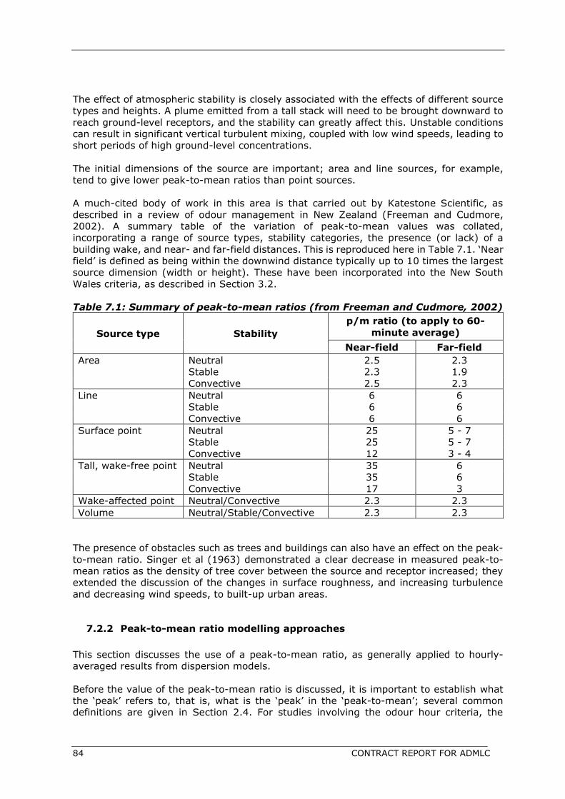
84 CONTRACT REPORT FOR ADMLC
The effect of atmospheric stability is closely associated with the effects of different source
types and heights. A plume emitted from a tall stack will need to be brought downward to
reach ground-level receptors, and the stability can greatly affect this. Unstable conditions
can result in significant vertical turbulent mixing, coupled with low wind speeds, leading to
short periods of high ground-level concentrations.
The initial dimensions of the source are important; area and line sources, for example,
tend to give lower peak-to-mean ratios than point sources.
A much-cited body of work in this area is that carried out by Katestone Scientific, as
described in a review of odour management in New Zealand (Freeman and Cudmore,
2002). A summary table of the variation of peak-to-mean values was collated,
incorporating a range of source types, stability categories, the presence (or lack) of a
building wake, and near- and far-field distances. This is reproduced here in Table 7.1. ‘Near
field’ is defined as being within the downwind distance typically up to 10 times the largest
source dimension (width or height). These have been incorporated into the New South
Wales criteria, as described in Section 3.2.
Table 7.1: Summary of peak-to-mean ratios (from Freeman and Cudmore, 2002)
Source type Stability
p/m ratio (to apply to 60-
minute average)
Near-field Far-field
Area Neutral 2.5 2.3
Stable 2.3 1.9
Convective 2.5 2.3
Line Neutral 6 6
Stable 6 6
Convective 6 6
Surface point Neutral 25 5 - 7
Stable 25 5 - 7
Convective 12 3 - 4
Tall, wake-free point Neutral 35 6
Stable 35 6
Convective 17 3
Wake-affected point Neutral/Convective 2.3 2.3
Volume Neutral/Stable/Convective 2.3 2.3
The presence of obstacles such as trees and buildings can also have an effect on the peak-
to-mean ratio. Singer et al (1963) demonstrated a clear decrease in measured peak-to-
mean ratios as the density of tree cover between the source and receptor increased; they
extended the discussion of the changes in surface roughness, and increasing turbulence
and decreasing wind speeds, to built-up urban areas.
7.2.2 Peak-to-mean ratio modelling approaches
This section discusses the use of a peak-to-mean ratio, as generally applied to hourly-
averaged results from dispersion models.
Before the value of the peak-to-mean ratio is discussed, it is important to establish what
the ‘peak’ refers to, that is, what is the ‘peak’ in the ‘peak-to-mean’; several common
definitions are given in Section 2.4. For studies involving the odour hour criteria, the
Efficacy of the different approaches in odour dispersion modelling
CONTRACT REPORT FOR ADMLC 85
definition of Cp should be the 90th percentile, but it is not always clear what is being
calculated in published studies.
Single peak-to-mean value
The most basic method for calculating peak concentrations is to apply a fixed, single peak-
to-mean value to the hourly mean concentrations.
An example of a fixed value for the peak-to-mean factor is the value of 4 required by odour
regulations in Germany, as used in AUSTAL, for example.
Brancher et al (2020b), using the data from the OROD field experiment, as described in
Section 6.2 of this report, tested the application of a fixed peak-to-mean value of 4. They
found that this approach led to an overprediction of the measured concentrations in all
cases, and hence they suggested that this could be used as a screening methodology, used
in order to determine whether further assessment with a more detailed methodology is
required. Brancher et al (2019) point out that many authors have reported that the
application of four as a constant peak-to-mean ratio tends to result in an overestimation
of odour hours in the field.
As described in Section 3.2, the guidance in the Australian state of Victoria prescribes the
use of a fixed peak-to-mean factor of 1.82, to convert to a 3-minute averaging time
(Victoria, 2013).
Many authors have questioned the effectiveness of using any single conversion factor.
Schauberger et al (2012), for example, categorically state that the body of evidence
demonstrating variation of peak-to-mean ratios in different situations convinces them that
the application of a constant factor for the ratio between the 90th percentile of the
instantaneous concentration and the hourly mean does not meet the requirements of
predicting odour annoyance. Olesen et al (2005) describe the use of a single factor as an
“extreme simplification”, and put forward an argument for the use of more sophisticated
models or algorithms within models that can estimate fluctuations in concentrations.
An interesting deviation from the simple rejection of the regulatory use of a single peak-
to-mean value is the observation by Janicke and Janicke (2004) and Oettl et al (2018a),
that using a fixed peak-to-mean value of 4 to calculate the 90th percentile of sub-hourly
averaged concentrations is actually a relatively good method, providing that a particular
parameter is within a certain range. This is a scale parameter in the equation to account
for the variation in odour sensitivities of individuals in odour panels, in field inspection
method VDI 3788 Part 1. In Section 6.5.2 of this report, ADMS was run using the dataset
described in the Oettl et al (2018a) article, and the model runs where a fixed peak-to-
mean of 4 was applied show good agreement with observations, for receptors more than
around 100 m from the sources. The article includes a detailed discussion of the range of
values of the scale parameter estimated for the odour dataset.
Variable peak-to-mean based on simple functions
Some modelling approaches are based on the application of a simple relationship to
calculate peak-to-mean ratios. Calculations for variable peak-to-mean ratios used in
several models, including CALPUFF, AODM and AUSPLUME, are based on the following
power-law function (e.g. Piringer et al, 2016; Brancher et al, 2017; Ferrero et al, 2020):
𝐶𝑝
𝐶𝑚
= (𝑡𝑚
𝑡𝑝
)
𝑛

86 CONTRACT REPORT FOR ADMLC
Where Cp is the peak concentration, Cm is the mean concentration, and tp and tm the
integration period for the peak and mean concentrations, respectively.
Brancher et al (2017) note that opinion varies on the most commonly applied value for the
exponent, n, with some authors claiming that this is 0.28 and others that it is 0.2. CALPUFF
also has an option to use this function to post-process the mean concentrations, and for
odour modelling, a value of 0.2 is advised for n.
Different values for n are sometimes used to take into account the atmospheric stability.
Schauberger et al (2012), for example, include a table of the maximum peak-to-mean
factors calculated from the above power-law equation by using values from Beychock
(1995) (denoted ‘Smith’ and ‘Trinity Consultants’ according to their original sources) and
values for tm and tp of 1 hour and 5 seconds, respectively. The values are reproduced here
in Table 7.2.
Table 7.2: Maximum peak-to-mean values calculated from exponents
Stability Class Smith Trinity Consultants
Exponent Cp/Cm Exponent Cp/Cm
Unstable 0.64 67.4 0.68 87.7
Slightly unstable 0.51 28.7 0.55 37.3
Neutral 0.38 12.2 0.43 16.9
Slightly stable 0.25 5.2 0.30 7.2
Stable 0 1 0.18 3.3
Very stable 0 1 0.18 3.3
Brancher et al (2020b) tested the methodology of varying the peak-to-mean ratio, by
varying the exponent in the power-law relationship described above. Literature exponent
values for different atmospheric stability classes were used (the ‘Trinity Consultants’
exponent values given in Table 7.2), with tm and tp set to 1 hour and 10 seconds,
respectively, in line with the experimental data; the resulting maximum peak-to-mean
ratio values were converted to 90th percentile equivalents, and simultaneously adjusted
according to receptor downwind distance, by means of a function put forward by Mylne
(1992), and Mylne and Mason (1991). They found that this approach showed a strong
tendency to underestimate the measured concentrations.
Venkatram (2002) questions the use of the above power-law formula, citing the fact that
its form suggests that the ensemble average is dependent on the averaging time of the
smaller timestep, although this is not actually the case. He suggests that the use of this
formula essentially just entails the use of an arbitrary factor to calculate a peak
concentration with no real physical meaning.
Other, slightly more complex relationships are sometimes used to calculate peak-to-mean
ratios, with terms to take into account factors such as the distance from the source and
the atmospheric stability, but these are ultimately still only rough approximations. More
sophisticated approaches involve the application of statistical concentration distributions,
and these are discussed in the next section.
7.2.3 Statistical approaches
Several publications include reviews of the statistical distribution properties of
concentration fluctuation datasets (e.g. Oettl and Ferrero, 2017; Cierco et al, 2012;
Cassiani et al, 2020). A table compiled by Efthimou et al (2016), and extended by Cassiani
Efficacy of the different approaches in odour dispersion modelling
CONTRACT REPORT FOR ADMLC 87
et al, provides a particularly useful list of key experimental studies and the respective
probability density functions (PDFs).
These reviews include summaries of seminal early research which involved testing various
PDFs against measured concentrations in several experimental datasets (e.g. Lewellen and
Sykes, 1986; Mylne and Mason, 1991; Yee et al, 1994).
The reviews of PDFs highlight the fact that these and subsequent studies found that
different experimental datasets were best described by different statistical distributions,
including clipped normal, log-normal, gamma, Wiebull and exponential, and it is useful to
explore the possible reasons why. As expected, the main reasons cited in the literature
include different downwind distances from the source, different source types and the
atmospheric stability.
The Lewellen and Sykes (1986) study involved the analysis of emissions from very tall
(200 m) power plant stacks. The measurements were carried out over a range of times of
day (including hours of darkness), and atmospheric conditions, and at distances of between
approximately 1 km and 20 km downwind of the stack. In contrast, the Mylne and Mason
(1991) studies involved three tracer release experiments carried out at three different
sites, over much shorter distances (50 to 1000 m) during near-neutral or slightly
convective conditions, mostly with a release height of 2 m, but some releases at ground-
level. Even though the source heights and downwind distances in the Mylne and Mason
experiments were very different to those in the Lewellen and Sykes work, and different
stability conditions were covered, the authors of both publications concluded that the data
were well represented by a clipped normal distribution.
Mylne and Mason further noted that, although the clipped normal PDF represented most of
their data well, this was not the case for distances very close to the source, where the
instantaneous plume was small in width and its dispersion was dominated by plume
meandering; the clipped normal distribution tended to underestimate concentrations, and
the exponential PDF often provided a better fit, in these very near field locations. For other
distances, though, and in general, they noted that the exponential PDF was less flexible
and often represented a very poor fit to the data.
Yee et al (1994) analysed data from tracer release experiments involving a point source
at a height of 2.5 m. They found that the shape of the PDF was highly dependent on the
location within the plume, both crosswind and downwind. At smaller distances downwind
(at, for example, around 50 m), they found that the PDF was ‘exponential-like’, with a
prominent frequency peak at zero concentration values due to the meandering of a narrow
instantaneous plume, and as downward distance increased (a few hundred metres), that
the distribution became bimodal, with a second frequency peak at non-zero concentrations
peak added to the peak at zero concentrations. At further distances still (at around 750 m),
the distribution became unimodal, with a single frequency peak at a non-zero concentration
value. It was found that a gamma distribution provided the best match for the non-zero
concentrations in the experimental data, and specifically, that this was particularly the case
when the plume was tending towards being more homogeneous; that is when the
downwind distances were greater and the atmospheric conditions were more stable.
Lung et al (2002) found that the concentration data from their tracer experiments was
effectively described by gamma and Weibull PDFs, but less so by a log-normal distribution.
All of the measurements were relatively close (< 100 m) to the ground-level point source,
and atmospheric conditions ranged from neutral to unstable.
Oettl and Ferrero (2017) tested several PDFs (2- and 3-parameter Weibull, gamma and
log-normal) against three field experiment datasets (the OROD dataset described in
88 CONTRACT REPORT FOR ADMLC
Section 6.2, data from the Sagebrush project (Finn et al, 2015), and data from the Joint
Urban 2003 experiment (Allwine and Flaherty, 2006). They found that all of the PDFs
underestimated the peak values, here defined as the 90th percentile of the sub-hourly
mean concentrations, and that, generally, the gamma PDF achieved the best overall fit to
the data. They found, however, that if they took the peak-to-mean values calculated from
the 2-parameter Weibull PDF and raised them to the power of 1.5, then this generated
reasonable peak concentration values.
Brancher et al (2020b) tried fitting measured data to gamma, lognormal, Weibull and
clipped normal PDFs, and found that there were large changes in the shape of the PDFs
over the different experiments and receptor locations and that, as a result, none of the
tested PDFs fit the entire range of the data effectively for all of the experiments. They did
find, however that the Gamma, Weibull and clipped normal PDFs were a reasonably good
fit to the data.
It seems reasonable to expect that it might be possible to draw out patterns from the
various studies, to find ‘universal’ PDFs that fit a majority of datasets, or at least identify
certain PDFs that can describe particular situations; and, to some degree, this has been
done.
Cassiani et al (2020) describe how many earlier studies indicated that the clipped normal
PDF provided a good fit to many datasets, although subsequent analysis suggested that
this PDF had limitations in describing the upper tail of the concentration distribution, and
the right skewness. They suggest that the findings of recent studies have tended towards
the gamma PDF being the best fit.
Examples to support this include the analysis of a water channel dataset by Yee and
Skvortsov (2011), where it was shown that the gamma PDF fitted data from a ground level
point source very well over the whole range of measured concentrations. Another example
is the work of Nironi et al (2015), whose point source concentrations in a wind tunnel
dataset were shown to be well represented by a gamma PDF over a range of source
elevations. Efthimiou et al (2016) found that the gamma PDF gave a good fit to the datasets
they studied, which focussed on urban settings, and on the upper tail of the concentration
distribution in particular.
But despite the many studies that demonstrate the good fit of the gamma PDF to several
datasets, it appears that there is, however, still no real consensus on a statistical
distribution that can be universally used to describe concentration fluctuations. Brancher
et al (2020b) describe the gamma function as versatile, but they also say “In fact, there is
still no broad agreement on which PDF fits concentration fluctuation data best”. Cierco et
al (2012), for example, also echo this: “The advantages of the different functions are not
clear enough to lead to general agreement”.
The range of distributions that fit different experimental data seems to suggest that
different distributions could better fit specific situations. It has been noted, for example,
that the gamma function seems to be unsuitable in the very near field, where the
concentration fluctuation intensity is highest, and that it does not seem to be applicable
for line sources (Cassiani et al, 2020). The same authors note that most field experiments
that involve fluctuating concentrations have involved point sources close to the ground,
and they recommend that more experiments should be carried out with elevated sources,
and over a range of stability conditions.
A key concept in the characterisation of concentration fluctuations is the ‘intermittency’,
which defines the time during which the concentrations at a receptor are zero, and
therefore describes the extent to which the concentrations occur in bursts. But, in practice,

Efficacy of the different approaches in odour dispersion modelling
CONTRACT REPORT FOR ADMLC 89
it is not possible to measure very low concentrations; for measurements, we are not really
considering ‘zero’ concentrations but concentrations below the detection limit of the
measurement technique, and this includes odour measurements by human panels. This
can have implications for the fitting of concentration distributions to PDFs (Cassiani et al,
2020).
Only a few models commonly used in the regulatory modelling of odours have the capacity
to calculate sub-hourly concentrations based on a PDF approach. The aforementioned
approach taken by Brancher et al (2020b), involving a Weibull PDF combined with a
concentration variance computation, has recently been incorporated into the GRAL model.
The fluctuations module in ADMS is based on a clipped normal PDF.
90 CONTRACT REPORT FOR ADMLC
7.3 Universal challenges in odour dispersion modelling
This section briefly explores those challenges and difficulties that are generally applicable
to odour dispersion modelling, and not specifically related to either of the broad categories
of odour criteria discussed in the previous two sections.
When discussing uncertainty in odour modelling, considerations such as building effects,
horizontal or covered releases and complex terrain are often raised (e.g. Sniffer, 2014).
These are, however, common factors in many applications of dispersion modelling, and are
not specific to odour, so are not considered here. Terrain and building effects occur in many
standard model validation datasets and studies, and non-standard sources such as
horizontal releases have been considered elsewhere (e.g. Stocker et al, 2015).
A key challenge, more specific to odour dispersion modelling, is the matter of emission
rates, and this remains an important point for discussion. There are two main options for
emission rates: the use of emission factors; and site-specific emission rates. For the
former, many people have called for centralised, comprehensive databases for odour
emission factors, to enable the sharing of the extensive information that is produced in the
large number of individual odour measurement assessments. Capelli et al (2014), for
example, put forward this recommendation, after reviewing the availability of odour
emission information for different sectors, including composting, wastewater treatment
and livestock operations.
There are existing official databases, such as that within the SCAIL-Agriculture tool (Sniffer
2014), which covers selected agricultural sources, and is updated as new information
becomes available, although the developers of the tool themselves call for further
improvements to odour emission factor data.
For the second option, of measured emission rates, there are several practical
considerations. It is, of course, not possible for proposed sites or activities, but even where
it is possible, there are many inherent difficulties in determining odour emission rates. It
can be physically impractical or dangerous to measure emissions from many odour
sources, and even when access is straightforward, the measurements of fugitive emissions
are notoriously difficult and prone to uncertainty, although this has improved in recent
years due to the widespread use of ‘directional’ (‘wind tunnel’) samplers.
Although it is outside the scope of this project to discuss the difficulty in adequately
characterising the source terms for some activities, such as fugitive emissions, this is,
nevertheless, often cited as a reason for poor agreement in validation studies (e.g. Ranzato
et al, 2012). This is not necessarily a problem that is inherent to the dispersion modelling
process itself (hence its exclusion from the scope), and the biggest barrier to effective
modelling is often due to a lack of relevant quantification of emissions. This is an example
of where progress outside the field of dispersion modelling could yield improvements in
odour impact prediction. Having said this, there is a further element to this discussion,
which is the use of inverse dispersion modelling techniques in helping to quantify fugitive
emissions. This has been carried out over small spatial scales for some time, and has been
further developed and applied over time (e.g. Schauberger et al, 2011; O'Shaughnessey
and Altmaeir, 2011; Capelli et al, 2013).
Another factor that is sometimes given as a reason for poor validation is cumulative odour.
Dispersion modelling studies usually only model sources from a single site, and sometimes
not all of the sources on a particular site (e.g. fugitive emissions are sometimes ignored).
This could explain, in some cases, some of the underestimation of odour impacts compared
with measurements. A dispersion modelling study by Naddeo et al (2012) has
demonstrated this clearly, with cumulative impacts from a wastewater treatment plant and
Efficacy of the different approaches in odour dispersion modelling
CONTRACT REPORT FOR ADMLC 91
an adjacent composting plant being shown to be much higher than the individual impacts,
both in terms of concentration magnitude and spatial extent.
In addition to the potential for straightforward linear additive effects of emissions, there is
also the more complex consideration of synergistic and masking effects of different types
of odour. As described in the validation section, Ranzato et al (2012) discuss the possibility
of additive effects in an area with several different odour sources, but they also discuss
the possibility that, when only one of the sources, the biofilter, was modelled, the
dispersion modelling predicted higher impacts close to the source than the field inspection,
due to the human participants only reporting the most unpleasant odour when multiple
types of odour were present.
As well as demonstrating the well-known difficulty in capturing temporal variation in
emissions, the work by Drew et al (2007) also highlights the less-discussed issue of spatial
variability, which can be of great importance in landfill sites, and other sites with large
sources with significant spatial heterogeneity.

92 CONTRACT REPORT FOR ADMLC
8 DISCUSSION
This report has considered odour criteria and dispersion modelling for the assessment of
odour annoyance, which can be generally divided into an hourly average concentration
approach and a sub-hourly average approach. Investigating the efficacy of these has
required different considerations for each approach. For the sub-hourly approach, the
significant inherent challenges associated with predicting sub-hourly concentrations in an
operational capacity mean that the method used to determine the peak concentration is a
dominant factor in whether odour annoyance is correctly predicted.
For the percentile of hourly average approach, a short averaging time is not required, and
this allows the other challenging aspects of odour modelling to come to the fore. These
challenges are also, of course, present for the sub-hourly approach of modelling, so many
of the issues discussed in this section of the report are therefore also relevant to the sub-
hourly assessment approach.
The review of existing validation studies has highlighted the scarcity of robust datasets
and studies that test the efficacy of the 98th percentile criteria and the associated
modelling methods, as well as the reasons for this. Historically it has been very difficult to
directly assess the criteria using standard validation datasets, as a whole year of ambient
hourly measurements would ideally be required. Costs and technology have been
understandably prohibitive. The emergence and dissemination of new technology in odour
monitoring and measurement is encouraging, with continuous measurements such as
electronic noses providing an opportunity for revisiting and expanding dose-response
studies, model validation and general elucidation of the quantification of odour nuisance
potential.
This technology will hopefully yield many more datasets for model comparison, and
facilitate many more odour studies. These should cover different types of odour-emitting
sectors, different types of sources, and more challenging types of emission, including non-
steady state and fugitive emissions in particular.
This development and widespread use of ambient odour monitoring should also help to
test the efficacy of criteria based on sub-hourly concentrations and odour hours, and of
the modelling methods involved. Further use of existing fluctuating plume datasets, such
as those from the Project Sagebrush experiments, could be made in the meantime.
A key question in the consideration of sub-hourly criteria is whether it is feasible and/or
appropriate to aim to model concentrations on very short timescales. The continued
relevance of this question is illustrated by the different positions held by different
authorities, even within single countries. In Australia, for example, several states have
criteria based on sub-hourly concentrations, while the Queensland odour guidance
maintains that the general understanding of peak-to-mean factors is considered to be
insufficient to justify setting criteria based on averaging times of less than an hour.
For all odour dispersion modelling research, there is a clear need for continuous, accurate
measurements to be coupled with detailed information on emissions, whether this is
measurements of emission rates, or activity data coupled with reliable emission factors.
In addition to the experimental datasets, further work is required to improve the ongoing
assessment of odour. An often repeated theme in the literature is that of emission rates
and a recognition that many emission rates used in odour modelling are not sufficiently
Acknowledgements
CONTRACT REPORT FOR ADMLC 93
accurate. It is apparent that development of databases of odour emission factors and other
similar resources would be welcomed by the odour dispersion modelling community. As
with the validation datasets, information on a range of sectors, source types and temporal
variation is needed.
It is likely that a multi-pronged approach is required to improve odour impact prediction
by dispersion modelling, including further validation, possible small modifications to the
odour criteria, and improvement in the representation of emission rates.
ACKNOWLEDGEMENTS
We would like to thank the operators of the Free Port of Riga, Latvia, BLB Baltijas Terminals
for the provision of the Riga Port dataset, and Dietmar Oettl, for the provision of the Styria
pig farm dataset.
We would also like to thank Steve Peirson, of ADAS, for reviewing the report
And finally, we would like to thank ADMLC for funding the work.

94 CONTRACT REPORT FOR ADMLC
REFERENCES
Aarhus University (2021) OML: Model description. https://envs.au.dk/en/research-
areas/air-pollution-emissions-and-effects/the-monitoring-program/air-pollution-
models/oml/oml-model-description/#Model-description-summary
Allwine, K.J. and Flaherty, J.E. (2006) Joint Urban 2003: Study overview and instrument
locations. Pacific Northwest National Laboratory. U.S. Department of Homeland Security
Alpha MOS (2015) Brochure: RQ Box solutions. Network of field-based electronic noses.
10292
Aubrun S. and Leitl, B. (2004) Unsteady characteristics of the dispersion process in the
vicinity of a pig barn. Wind tunnel experiments and comparison with field data.
Atmospheric Environment, 38, 81-93.
Bachlin, W. et al (2002) (Provision of Validation Data for Odour Disposal Models - Field
Measurements). Research report FZKA-BWPLUS
Baumann-Stanzer, K. et al (2008). User experience with model validation exercises.
Croatian Meteorological Journal. 43. 52-56
Beychok, M. R. (1995) Fundamentals of Stack Gas Dispersion. Third edition
Brancher, M. et al (2017) A review of odour impact criteria in selected countries around
the world. Chemosphere, 168, 1531-1570
Brancher, M. et al (2019) Do odour impact criteria of different jurisdictions ensure
analogous separation distances for an equivalent level of protection? Journal of
Environmental Management, 240, 394-403
Brancher, M. et al (2020a). Temporal variability in odour emissions: To what extent this
matters for the assessment of annoyance using dispersion modelling. Atmospheric
Environment: X, 5, 100054
Brancher, M. et al (2020b) Performance evaluation of approaches to predict sub-hourly
peak odour concentrations. Environment: X, 5, 100076.
Bokowa, A. et al (2021) Summary and Overview of the Odour Regulations Worldwide.
Atmosphere, 12, 206
Bull, M. et al (2014). IAQM Guidance on the assessment of odour for planning, Institute of
Air Quality Management.
Bull, M.A. and Fromant, E.L. (2014) The performance of numerical odour assessment for
the prediction of odour complaints from wastewater treatment works. Water and
Environment Journal, 28, 316–322
Capelli, L. et al (2013) Measuring odours in the environment vs. dispersion modelling: A
review. Atmospheric Environment, 79, 731-743
Capelli L. et al (2014) Odour emission factors: fundamental tools for air quality
management, Chemical Engineering Transactions, 40, 193-198
References
CONTRACT REPORT FOR ADMLC 95
Capelli, L. and Sironi, S. (2018) Combination of field inspection and dispersion modelling
to estimate odour emissions from an Italian landfill. Atmospheric Environment 191, 273–
290
Carpentieri, M. et al (2008) Modelling tracer dispersion from landfills. Environmental
Modelling & Assessment, 13, 3, 415-429
Cassiani, M. et al (2020) Concentration fluctuations from localized atmospheric releases.
Boundary-Layer Meteorology, 177, 461–510
CEN (2003) EN 13725 Air quality - Determination of odour concentration by dynamic
olfactometry.
CEN (2016a) EN 16841-1 Ambient air - Determination of odour in ambient air by using
field inspection - Part 1: Grid method
CEN (2016b) EN 16841-2 Ambient air - Determination of odour in ambient air by using
field inspection - Part 2: Plume method
CERC (2016) ADMS 5 Atmospheric Dispersion Modelling System User Guide. Cambridge
Environmental Research Consultants. Version 5.2. November 2016.
Chirmata, A. and Ichou, I.A. (2016) Odour Impact Assessment by means of dispersion
modeling, dynamic olfactometry and mobile electronic nose around Agadir fishing port in
Morocco. Journal of Environmental Protection, 7, 1745-1764.
Cierco, F-X. (2012) Modelling concentration fluctuations for operational purposes,
International Journal of Environment and Pollution, 48, 1/2/3/4, 78–86
CSIRO (2008) TAPM V4. Part 1: Technical Description. CSIRO Marine and Atmospheric
Research Paper No. 25
Davies BM, et al (1998) Some field experiments on the interaction of plumes from two
sources. Quarterly Journal of the Royal Meteorological Society, 126, 565, 1343-1366
Dourado, H.O. et al (2013). Validation of Gaussian models using wind tunnel experiments
and numerical simulation. In: HARMO 15: 15th International Conference on Harmonisation
within Atmospheric Dispersion Modelling for Regulatory Purposes, Madrid.
Dousa (2019). Comparison Access to Odor Problems in Selected European Countries.
Journal of the Polish Mineral Engineering Society, 21, 1, 83-87
Drew, G.H. (2007) Appropriateness of selecting different averaging times for modelling
chronic and acute exposure to environmental odours. Atmospheric Environment 41, 2870–
2880
Efthimou, G. C. et al (2016) Prediction of the upper tail of concentration distributions of a
continuous point source release in urban environments. Environmental Fluid Mechanics
(2016) 16:899–921
Elbir, T. et al. (2007) Evaluation of Measured and Predicted Odor Concentrations around
a Meat Packaging and Rendering Plant. Environmental Engineering Science, 24, 3

96 CONTRACT REPORT FOR ADMLC
Environmental Protection Agency (2001) Odour Impacts and Odour Emission Control
Measures for Intensive Agriculture. Final Report. R&D Research Report 14. Ireland
Environment Agency (2002). Assessment of Community Response to Odorous Emissions.
R&D Technical Report: P4-095/TR. UK
Environment Agency (2007a). Review of odour character and thresholds. Science Report:
SC030170/SR2. UK
Environment Agency (2007b). Review of dispersion modelling for odour predictions.
Science Report: SC030170/SR3. UK
Environment Agency and Natural Resources Wales (2019). Specified generators:
dispersion modelling assessment. https://www.gov.uk/guidance/specified-generators-
dispersion-modelling-assessment#results-and-impact-assessment
Estonia (2016) The Regulation of the Minister of Environment No. 81 (27.12.2016)
‘Procedures for assessing the appearance of odour, evaluation requirements and levels of
odour’.
Fackrell, J.E. and Robins, A.G. (1982) The effects of source size on concentration
fluctuations in plumes. Boundary-Layer Meteorology, 22, 335–350
Ferrero, E. et al (2020) Concentration Fluctuations and Odor Dispersion in Lagrangian
Models. Atmosphere, 11, 27
Finn, D. et al (2015) Project Sagebrush Phase 1. NOAA Technical Memorandum OAR ARL-
268
Freeman, T. and Cudmore, R. (2002). Review of Odour Management in New Zealand. Air
Quality Technical Report 24
Germany (2008) Feststellung und Beurteilung Von Geruchsimmissionen
(Geruchsimmissions-Richtlinie - GIRL)
Germany (2015) VDI 3788 Part 1. Environmental meteorology - Dispersion of odorants in
the atmosphere – Fundamentals.
Griffiths, K.D. (2014) Disentangling the frequency and intensity dimensions of nuisance
odour, and implications for jurisdictional odour impact criteria. Atmospheric Environment,
90, 125-132
Hanna, S.R. (1984) Concentration fluctuations in a smoke plume. Atmospheric
Environment, 18, 1091-1106
Henry, C.G. et al (2010) Ground truthing CALPUFF and AERMOD for odor dispersion from
swine barns using ambient odor assessment techniques. Agricultural and Biosystems
Engineering Conference Proceedings and Presentations, 303
Hong et al. (2011) CFD modelling of livestock odour dispersion over complex terrain, part
II: Dispersion modelling. Biosystems Engineering, 108, 265-279
Ireland (2019a) EPA, Office of Environmental Enforcement. Odour Emissions Guidance
Note (Air Guidance Note AG9)
References
CONTRACT REPORT FOR ADMLC 97
Ireland (2019b) EPA, Office of Environmental Enforcement (2019) Air Guidance Note 5
(AG5) Odour Impact Assessment Guidance for EPA Licensed Sites
Ireland (2020) EPA, Office of Environmental Enforcement. Air Dispersion Modelling from
Industrial Installations Guidance Note (AG4)
Janicke Consulting (2021) https://www.janicke.de/en/lasat.html
Janicke Consulting and UBA (2014) AUSTAL2000 Program Documentation of Version 2.6.
26/06/2014
Janicke, L. and Janicke, U. (2007) The development of the dispersion model AUSTAL2000G.
Janicke Consulting.
Keder, J. (2008), Adaptation of the Czech regulatory dispersion model for odour dispersion
calculation, its validation and critical evaluation. Chemical Engineering Transactions, 15.
Langner, C. and Klemm, O. (2011) A Comparison of Model Performance between AERMOD
and AUSTAL2000. Journal of the Air & Waste Management Association, 61:6, 640-646.
Latvia (2014). Regulation of Cabinet of Ministers No. 724 (25.11.2014) Regulations
Regarding the Methods for Determination of the Odours Caused by Polluting Activity, as
well as the Procedures for Restricting the Spread of such Odours
Lewellen, W. and Sykes, R. (1986) Analysis of concentration fluctuations from LIDAR
observations of atmospheric plumes. Journal of Climate and Applied Meteorology, 25,
8,1145–1154
Lithuania (2010) Lithuanian Hygiene Norm HN 121:2010 Odour concentration threshold in
the air of living environment, approved by order No. V-885.
Lombardy (2012) Determinazioni generali in merito alla caratterizzazione delle emissioni
gassose in atmosfera derivanti da attività a forte impatto odorigeno
Lung, T. et al (2002) Measurements and modelling of full-scale concentration
fluctuations. Agratechnische Forsch 8:5–15
Miedema, H.M.E. et al (2000) Exposure-annoyance relationships for odour from industrial
sources. Atmospheric Environment, 34, 2927-2936
Mylne, K.R. and Mason, P. (1991) Concentration fluctuation measurements in a dispersing
plume at a range of up to 1000 m. Quarterly Journal of the Royal Meteorological Society
117,497,177–206
Mylne, K.R. (1992) Concentration fluctuation measurements in a plume dispersing in a
stable surface layer. Boundary-Layer Meteorology 60, 1, 15–48
Naddeo, V. et al (2012) Odour Impact Assessment in Industrial Areas. Chemical
Engineering Transactions, 30, 85-90
New South Wales (2006a) Air Policy Section of the Department of Environment and
Conservation. Technical framework: Assessment and management of odour from
stationary sources in NSW

98 CONTRACT REPORT FOR ADMLC
New South Wales (2006b) Air Policy Section of the Department of Environment and
Conservation. Technical notes: Assessment and management of odour from stationary
sources in NSW.
New South Wales (2017) Environment Protection Authority. Approved methods for the
modelling and assessment of air pollutants in NSW.
New Zealand (2016) Ministry for the Environment. Good Practice Guide for Assessing and
Managing Odour. ME 1278.
Nironi, C. et al (2015) Dispersion of a Passive Scalar Fluctuating Plume in a Turbulent
Boundary Layer. Part I: Velocity and Concentration Measurements. Boundary-Layer
Meteorology, 156, 415–446
OdourNet and EPA Ireland (2001) Odour Impacts and Odour Emission Control
Measures for Intensive Agriculture
Oettl, D. and Ferrero, E. (2017) A simple model to assess odour hours for regulatory
purposes. Atmospheric Environment, 155, 162-173
Oettl, D. et al (2018a). Odour assessment in the vicinity of a pig-fatting farm using field
inspections (EN 16841-1) and dispersion modelling. Atmospheric Environment, 181, 54-
60.
Oettl, D. et al (2018b). Towards a Harmonized Odour Guideline for Some Austrian
Provinces. Chemical Engineering Transactions, 68.
Oettl, D. (2021) Documentation of the Lagrangian Particle Model GRAL-SCI (Graz
Lagrangian Model). Version 21.1. Government of Styria. January 2021.
Olesen, H.R. et al (2005) National Environmental Research Institute (NERI). Ministry of
the Environment. Regulatory odour model development: Survey of modelling tools and
datasets with focus on building effects. NERI Technical Report No. 541
O’Shaughnessey, P. T. and Altmaeir, R. (2011) Use of AERMOD to determine a hydrogen
sulfide emission factor for swine operations by inverse modelling. Atmospheric
Environment, 45, 27, 4617-4625
Piringer, M. et al (2007) A sensitivity study of separation distances calculated with the
Austrian Odour Dispersion Model (AODM). Atmospheric Environment, 41, 1725- 1735
Piringer, M. et al (2016). Factors influencing separation distances against odour annoyance
calculated by Gaussian and Lagrangian dispersion models. Atmospheric Environment, 140,
69-83.
Puglia (2018). Legge Regionale 16 luglio 2018, n. 32 “Disciplina in materia di emissioni
odorigene”. Bollettino Ufficiale della Regione Puglia - n. 96 suppl. del 19-7-2018.
Queensland (2011). Best Practice Guidance for the Queensland Poultry Industry – Plume
Dispersion Modelling and Meteorological Processing
Queensland (2013) Department of Environment and Heritage Protection. Guideline: Odour
Impact Assessment from Developments.

References
CONTRACT REPORT FOR ADMLC 99
Queensland (2016) Department of Agriculture and Fisheries. Development of Meat Chicken
Farms in Queensland.
Ramsdell, J.V. (1971). Concentration fluctuations and peak-to-mean concentration ratios
in real plumes. Atmospheric Sciences Department, Pacific Northwest Laboratories.
Proceedings of Air pollution, turbulence and diffusion symposium, Las Cruces, New Mexico.
BNWL-SA-4095
Ranzato, L. et al (2012). A comparison of methods for the assessment of odor impacts on
air quality: Field inspection (VDI 3940) and the air dispersion model CALPUFF. Atmospheric
Environment, 61, 570-579
Rossi, A.N. et al (2018). Update on the Italian Regulation about Odour Emissions and
Impact and Future Perspectives. Chemical Engineering Transactions, 68
Satler, M. and Devanathan, S. (2007) Which meteorological conditions produce worst-case
odors from area sources? Journal of the Air & Waste Management Association, 57, 11,
1296-1306
Schauberger, G. et al (2001) Model Calculation of Odour Sensation in the Vicinity of a
Livestock Building: a Meteorological Analyses when Odour Occur. Water Science &
Technology, 44, 9, 43-51
Schauberger, G. et al (2011). Odour emissions from a waste treatment plant using an
inverse dispersion technique. Atmospheric Environment, 181, 1639-1647.
Schauberger, G. et al (2012). Concept to assess the human perception of odour by
estimating short-time peak concentrations from one-hour mean values. Reply to a
comment by Janicke et al. Atmospheric Environment, 45, 624-628.
Schauberger G. and Piringer M. (2015) Odour impact criteria to avoid annoyance. Austrian
Contributions to Veterinary Epidemiology, 8, 35-42
Scotland (2010). Scottish Environmental Protection Agency and Natural Scotland. Odour
guidance.
Singer, I. A. (1961) The relationship between peak and mean concentrations. Journal of
the Air Pollution Control Association, 11, 7, 336-341.
Singer, I. A. (1963) Peak to mean pollutant concentration ratios for various terrain and
vegetation cover. Journal of the Air Pollution Control Association, 13, 1, 40-42
Sironi, S. et al (2010) Odour impact assessment by means of dynamic olfactometry,
dispersion modelling and social participation. Atmospheric Environment, 44, 354-360
Sniffer (2014) SCAIL Agriculture. Sniffer ER26: Final Report
South Australia (2016a) Environment Protection Authority. Ambient air quality
assessment.
South Australia (2016b) Environmental Protection (Air Quality) Policy. Version: 1.9.2016
Stocker, J. (2015) A review of the limitations and uncertainties of modelling pollutant
dispersion from non-point sources. ADMLC report. ADMLC 2015/06
100 CONTRACT REPORT FOR ADMLC
Tasmania (2004) Environment Protection Authority. Environment Protection Policy (Air
Quality).
United Kingdom (2011) Environment Agency. H4 Odour Management – how to comply with
your environmental permit.
United Kingdom (2002) Environment Agency. Horizontal Guidance for Odour Part 2 –
Assessment and Control
USEPA (2017) Revisions to the Guideline on Air Quality Models: Enhancements to the
AERMOD Dispersion Modeling System and Incorporation of Approaches to Address Ozone
and Fine Particulate Matter. Federal Register Vol. 82, No. 10. January 2017.
USEPA (2021) User's Guide for the AMS/EPA Regulatory Model (AERMOD). EPA-454/B-21-
001. April 2021
USEPA (2021) https://www.epa.gov/scram/air-quality-dispersion-modeling-alternative-
models#calpuff
Van Elst T. and Delva J. (2016), The European standard pren 16841-2 (determination of
odour in ambient air by using field inspection: plume method): a review of 20 year
experience with the method in Belgium. Chemical Engineering Transactions, 54, 175-180
Venkatram, A. (2002) Accounting for averaging time in air pollution modelling.
Atmospheric Environment, 36, 2165–2170
Victoria (2001) Government Gazette. No. S 240 Friday 21 December 2001
Victoria (2002) Environment Protection Authority. AUSPLUME for Windows
Air modelling software for industry. Information Bulletin.
Victoria (2013) Environment Protection Authority. Guidance notes for using the regulatory
air pollution model AERMOD in Victoria. Publication 1551.
Victoria (2017) Environment Protection Authority Odour environmental risk assessment for
Victorian broiler farms. Publication 1643.
Vieira de Melo, A.M. et al. (2012). Modelling of odour dispersion around a pig farm building
complex using AERMOD and CALPUFF. Comparison with wind tunnel results. Building and
Environment, 56, 8-20
Wang, L. et al (2006). Comparison of CALPUFF and ISCST3 models for predicting downwind
odor and source emission rates. Atmospheric Environment, 40, 4663-4669
Western Australia (2019). Department of water and Environmental Regulation. Guideline:
Odour emissions
Yee, E. et al (1994) Experimental measurements of concentration fluctuations and scales
in a dispersing plume in the atmospheric surface layer obtained using a very fast response
concentration detector. Journal of Applied Meteorology 33, 8, 996–1016
Yee, E. and Skvortsov, A. (2011) Scalar fluctuations from a point source in a turbulent boundary layer. Physical Review E, 84, 3, 036306

References
CONTRACT REPORT FOR ADMLC 101
Yu, Z. et al (2011). Development of a Livestock Odor Dispersion Model: Part II. Evaluation
and Validation. Journal of the Air & Waste Management Association, 61, 277–284