Adjustment method of an imaging Stokes polarimeter based on liquid crystal variable retarders

Adjustment method of an imaging Stokes polarimeterbased on liquid crystal variable retarders

Władysław A. Woźniak,* Piotr Kurzynowski, and Sławomir DrobczyńskiInstitute of Physics, Wrocław University of Technology, Wybrzeże Wyspiańskiego 27, 50-370 Wrocław, Poland

*Corresponding author: [email protected]

Received 27 October 2010; accepted 22 November 2010;posted 30 November 2010 (Doc. ID 137222); published 7 January 2011

The description of adjustment of an imaging Stokes polarimeter constructed and tested in our laboratoryis presented. Our polarimeter’s operation is based on six fast intensity distribution measurements rea-lized in six different configurations of linear and circular analyzers. Using liquid crystal variable retar-ders (LCVRs) makes this construction compact and mechanically simple. However, new problems arisewith proper azimuthal alignment as well as with proper LCVR voltage adjustment. Three basic steps ofthe adjustment procedure adapted to the specific construction of our polarimeter are described in detail.Some remarks concerning the critical parameters of the used CCD camera’s parameters are alsopresented, as well as experimental verifications of the setup’s accuracy acquired due to the properadjustment process. © 2011 Optical Society of AmericaOCIS codes: 120.5410, 230.0230.

1. Introduction

The intensity distribution measurement of the inves-tigated light belongs to one of the most common mea-surements in optics. However, another parameterplays an even more important role in interferome-try—phase distribution (intensity distribution couldalso be helpful in many cases). The third set of para-meters, which falls within the interest of many opti-cians, consists of the polarization parameters, suchas azimuth and ellipticity angles, as well as polariza-tion degree. The light polarization state measure-ments play an important role in many fields ofresearch, such as polarimetric testing of optoelectro-nic devices, and photoelasticity.

Several polarimetric systems with different con-struction principles have been proposed so far [1–4],starting from the static method in which only a fewintensities are measured and finishing with the dy-namic method in which several full intensity charac-teristics are needed. Some of these methods used theinterferometric configurations [5,6], while others usethe Fourier transform [7–9]. Older constructions

were based on mechanically rotated polarization ele-ments. The new ones used liquid crystal variable re-tarders (LCVRs) [10–13]—some, in fact, even againproposed static setups using a system of special bire-fringent prisms [14–16]. The final results of the mea-surements could be obtained in a direct way, as a setof light polarization parameters, or indirectly, bymeasuring the Stokes parameters of the light(commonly called “Stokes polarimeters” [17,18]).Generally, constructions of all polarimetric setupstend to increase the accuracy of measurement andto automatize the measurement process, as well asdesign small, compact devices without mechanicallyrotating elements. Stokes polarimeters based onLCVRs are a good example of this.

In the present paper, we are describing a compactand simple realization of such a type of polarimeterconsisting of two LCVRs and one linear analyzer in“static” configuration. In fact, we are not concentrat-ing on the setup itself—this is only one possiblerealization among many others proposed in the lit-erature. Therefore, we conclude that the descriptionof some practical problems connected with proper ad-justment of LCVRs used could be of much interest.LCVRs are key components of modern measurement

0003-6935/11/020203-10$15.00/0© 2011 Optical Society of America

10 January 2011 / Vol. 50, No. 2 / APPLIED OPTICS 203

systems and many authors have characterized theirperformance and orientation problems in terms ofmodulation precision as well as image quality [19–21]. Thus, we present a method of the setup adjust-ment, as well as some problems connected with theproper selection of CCD camera parameters. We par-ticularly describe a method for the angular arrange-ment of both LCVR elements and the process of theproper selection of the input voltages. We hope thatthis detailed description helps the reader in con-structing similar measurement devices. To prove theacquired accuracy of the described setup, the exemp-lary results of the measurements and error analysisof the obtained results are presented.

2. Polarimeter Setup

The scheme of the proposed Stokes polarimeter ispresented in Fig. 1. Our polarimeter consists oftwo LCVRs (LRC-200, Meadowlark Optics) and onelinear polarizer (LPVIS100-MP, Thorlabs), which,placed beyond both LCVRs, is called an analyzer.The CCD camera allows acquiring x–y-intensity dis-tributions at the output plane of the setup for six cho-sen sequences of LCVR retardations. The angularorientations of the fast axes of all the three polariza-tion elements are also presented in Fig. 1.

The chosen angular orientations of both LCVRsand the analyzer A allow establishing several differ-ent analyzers and recording the x–y-intensity distri-butions at the output plane of the setup. Therecould be many possible combinations of selectedorientations, as well as of the proper retardations in-troduced by both LCVRs to obtain the desired aim—

measurement of four Stokes components of polarizedlight. It is easy to show that the set of four analyzersestablished an absolute minimum to obtain completeinformation about all four Stokes parameters. How-ever, to increase themeasurementaccuracy andmakethe computation process simpler and intuitive, wehave chose a very specific set of six analyzers: thepoints representing the analyzers lie on the six “poles”on the Poincaré sphere [22] and represent four linearpolarizers with azimuth angles equal to 0°ð~V0Þ, 90°ð~V90Þ, 45°ð~V45Þ, and −45°ð~V

−45Þ, and two circular oneswith ellipticity angles equal to þ45° (~VR, right-

handed) and −45° (~VL, left-handed). The retardationsγLCVR1 and γLCVR2 introduced by both LCVRs for thechosenset of analyzersare shown inTable1.Note thatthis selection also enables precise alignment of thesetup (shown in Section 3).

As wasmentioned before, themain aim of our workis to present the adjustment method of the proposedStokes polarimeter rather than a detailed descrip-tion of the setup itself. However, the knowledge ofmathematical formulas used to calculate all desiredparameters of polarized light could be helpful in un-derstanding the principles of the adjustment process.

If we denote the Stokes vector components of theexamined light as ~Vðx; yÞ ¼ ðV1;V2;V3;V4Þ, thenthe formulas for all these components can be writtenas follows:

V1 ¼ I0 þ I90 ¼ I−45 þ I45 ¼ IR þ IL; ð1Þ

V2 ¼ I0 − I90I0 þ I90

; ð2Þ

V3 ¼ I45 − I−45

I45 þ I−45

ð3Þ

V4 ¼ IR − ILIR þ IL

: ð4Þ

(Note that all the quantities in the above equationsare x–y-distributions). Even though the V1ðx; yÞparameter can be deduced from the knowledge ofonly two chosen intensity distributions, we usedall six measured intensities to increase the accuracyof this important quantity. Let us also emphasize thespecific form of the last three formulas, in which theintensity obtained from combinations of the orthogo-nal pair of proper analyzers was used. This charac-teristic feature of the proposed setup is alsoimportant from the proper LCVR adjustment’s pointof view.

Finally, the polarization parameter distributionsof the examined light can be calculated from the fol-lowing formulas:

Table 1. Sequence of Retardations γLCVR1 and γLCVR2 Introduced by BothLCVRs for the Chosen Set of Analyzer

Stokes Eigenvector of theAnalyzer

γLCVR1(°)

γLCVR2(°)

MeasuredIntensity

~V0 0 0 I0~V90 0 180 I90~VR 0 90 IR~VL 0 270 IL~V45 180 0 I

−45~V

−45 180 180 I45

Fig. 1. Scheme of the optical system of the proposed Stokespolarimeter: LCVR1, LCVR2, liquid crystal modulators; A, linearanalyzer; CCD, camera.

204 APPLIED OPTICS / Vol. 50, No. 2 / 10 January 2011

– mean intensity

Iðx; yÞ ∝ V1 ¼ I0 þ I90 ¼ I−45 þ I45 ¼ IR þ IL; ð5Þ

– polarization degree

pðx; yÞ ¼ffiffiffiffiffiffiffiffiffiffiffiffiffiffiffiffiffiffiffiffiffiffiffiffiffiffiffiffiffiffiV2

2 þ V23 þ V2

4

q; ð6Þ

– azimuth angle

αðx; yÞ ¼ 0:5 · arctan�V3

V2

�; ð7Þ

– ellipticity angle

ϑðx; yÞ ¼ 0:5 · arcsinðV4Þ: ð8Þ

The ratio sign used in Eq. (5) denotes that, in fact,we have measured the intensity of light emergingfrom our measurement setup, which is proportionalto the input light. Admittedly, in this way we do notmeasure the absolute value of the light intensity, butthe relative changes in Iðx; yÞ distribution still can beobserved. Taking into account that this undisclosedratio coefficient is present in all four Stokes para-meters, we can measure the polarization degree ac-cording to Eq. (6). Let us also note that, to omit theproblems connected with unwrapping the azimuthangle distribution in our computational program,we used the complete information about the para-meters V2 and V3 instead of the ratio ðV3=V2Þ.3. Adjustment of Liquid Crystal Variable Retarders

The azimuthal adjustment of the LCVRs as well asthe proper choice of the voltage necessary to obtainthe desired retardations γLCVR1 and γLCVR2 determinethe possible accuracy obtained in our setup. Thus, wedivided the adjustment process into three steps (foreach analyzer). The critical assumption of all adjust-ment processes is the linear response of the CCDcamera. Other problems emerge at the crossroadsof optics and electronics, which will be discussed indetail in Section 4.

A. Step (a): Preliminary Voltage Adjustment

The very two first steps are the measurements of thefull intensity versus voltage characteristics for bothLCVRs in a polariscopic setup (a crossed linear polar-izer and an analyzer) and approximation of theobtained data according to Malus law. Formally, thisstep requires proper angular alignment of theLCVRs (with azimuth angle αLCVR ¼ 45° accordingto azimuth angles of the crossed linear polarizerand the analyzer, assumed to be equal to 0° and90°, respectively). However, the character of the in-tensity versus voltage characteristic does not evenchange for αLCVR mismatch, which allows obtainingthe proper values of specific voltages for both LCVRs

with sufficient accuracy. These approximate charac-teristics would be a good base for selecting the initialvalues of the input voltages for both LCVRs, which isessential to obtaining the desired value of the intro-duced retardations.

B. Step (b): Precise Voltage and Angular Adjustment in aPolariscopic Setup

The next step of the adjustment was also made in apolariscopic setup consisting of a fixed linear polar-izer (azimuth angle equal to 0°), an adjusted LCVR, alinear analyzer with changeable azimuth angle, andan additional achromatic quarter-wave plate. Still,we adjusted both LCVRs separately, which couldgenerate some errors [see Step (c) below]. Generally,this stage of the adjustment process relied upon find-ing out the proper voltages to obtain absolute mini-mums of the signal at the setup’s output for the set ofselected analyzer positions. The adjustment of thefirst LCVR’s proper voltages to obtain linear analy-zers ~V0, ~V90, ~V45, and ~V

−45 was, in general, much ea-sier than in the case of the circular ones (~VR, ~VL)—now, to obtain the same minimums of the intensity,we were forced to use additionally calibrated achro-matic quarter-wave plates.

The intensity versus voltage characteristics ob-tained in Step (a) are generally strongly nonlinear.The dependence of the phase difference introducedby LCVR on input voltage is the strongest for phasedifference γLCVR1 near 180°, while the characteristiccurve is for γ ¼ 0° almost flat. So the first critical stepof the adjustment—the angular orientation of theLCVRs azimuth angle αLCVR1 ¼ 45°—was done forthe voltage value corresponding to γLCVR ¼ 180°(~V90 analyzer) obtained from Step (a). Now boththe polarizer and the analyzer were set on azimuthangle equal to 0°. The absolute minimum of the lightcould be observed only for αLCVR1 ¼ 45° and γLCVR1 ¼180° obtained simultaneously. Note that both theseLCVR parameters enter the intensity formula multi-plicatively so that the procedure of obtaining theoutput signal’s absolute minimum is convergent.This way, the proper value of LCVR azimuth angle(αLCVR1 ¼ 45°) is obtained and fixed for the rest ofthe adjustment substeps. Next, the proper value ofthe input voltage for γLCVR1 ¼ 0° (~V0 analyzer) canbe obtained in the same way, rotating the analyzerto azimuth angle equal to 90° (classical cross config-uration) and finding the absolute minimum of theoutput intensity in the configuration. Bearing inmind the remark about the flatness of intensity ver-sus voltage (and, finally, phase difference versus vol-tage) characteristics, one can find this voltageadjustment most imprecise. In fact, the possibilityof finding the proper voltage in this case is difficultalso because it strongly depends on the quality of thecorrection wave plate (originally integrated with theLCVRs) used to ensure the absolute value of γ ¼ 0°.The principles of liquid crystal retarders construc-tions cause that, even for very high input voltage,there still exist residual birefringences connected


with the liquid crystal molecules’ initial orientation.However, laboratory practice convinced us that thepotential errors in obtaining absolute γ ¼ 0° valueare not so critical.

More critical is finding the proper values of the in-put voltage for two circular configurations of ourproposed analyzers (~VR and ~VL). Again, there is nopossibility of obtaining the minimum intensity forsuch phase differences (90° and 270°, respectively)using only, like in previous steps, a linear polarizerand an analyzer. Taking into account the basic con-cept of finding absolute minimums of intensity as adeterminant of proper alignment, we decided to usean additional element—the achromatic quarter-wave plate—as a specimen. Both the LVCR andthe quarter-wave plate were placed inside the classi-cal polarization cross (the linear polarizer with azi-muth angle equal to αP ¼ 0° and the analyzer withαA ¼ 90°), with azimuth angles equal to �45° (fastaxis of the LCVR is parallel to the fast or slow oneof the quarter-wave plate). Now the adjustment pro-cedure relies on finding such LCVR voltages forwhich the LCVR compensates the phase shift intro-duced by the quarter-wave plate in both azimuthalalignments. Knowing that the azimuth angle ofLCVR1 is fixed to 45°, which was precisely arrivedat during the first substep (~V90 analyzer’s adjust-ment), only the quarter-wave plate was slightlyrotated at this stage. And again, an additional degreeof freedom during this adjustment procedure is theazimuth angle of the specimen—subtle angularmovement of the quarter-wave plate around themanufactured marker of the fast (slow) axis can helpin obtaining the desired minimum of intensity at theoutput.

The adjustment process of the second retarder(LCVR2) for the ~V45 and ~V

−45 is the same as thatof the first one (LCVR1) for ~V90 and ~V0. The only twodifferences are (1) the azimuth angles of LCVR2,which should be equal to the uncommon value ofαLCVR2 ¼ 22:5°, and (2) the position of the analyzer(0° or 45°) for which the absolute minimums of inten-sities were reached. We did not use any precise scaleto find the 22:5° value—as it was previously de-scribed, the procedure of finding azimuthal orienta-tion and proper value of the voltage can be donesimultaneously.

As described above, this adjustment stage is basedon finding the absolute minimum of the output lightintensity in different polariscopic configurations. Sothe possibility of the minimum determination couldbe assured. We used the visual observation of the sig-nal on the monitor, as well as an independent power-meter. However, to obtain the most satisfactoryresults and increase the accuracy of the determinedminimum, we were forced to temporarily modify theparameters of the CCD camera and electronicallyamplify the obtained signal, as well as increasethe intensity of the input light. Let us note thatthe overexposed image registered by the CCD cam-

era hasmade this instrument evenmore precise thanthe classical powermeter.

C. Step (c): Final Verification of the Complete SetupAdjustment Quality

The main defect of the described above procedures isthe fact that both LCVRs were adjusted indepen-dently. Formally, if the both liquid crystal elementsare properly oriented regarding the azimuth angleand the voltages are properly selected, then the pre-sence of the one LCVR should not affect the secondone’s functioning. However, we can confirmmany im-perfections of the manufactured LCVRs reportedalso by other authors [21]. So we decided to verifythe proper azimuth orientations and voltage assort-ment in a complete Stokes polarimeter setup consist-ing of two LCVRs and a linear analyzer. As the thirdstep, wemeasured all the component intensity distri-butions I0, I90, I−45, I45, IR, and IL for some specificinput lights and made the final subtle correctionsof the azimuthal alignments, as well as of the bothLCVRs’ voltages. The exemplary results of this stageare shown in Fig. 2.

The measurement of all the intensities I0, I90, I45,I−45, IR, and IL in the described measurement weredone for the linearly polarized input light with theazimuth angle equal to 0°, linear analyzer A withthe azimuth angle also equal to 0°, while LCVRswere adjusted to retardations γLCVR1 ¼ 0° and γLCVR1¼ 180°. According to the theory, the final resultsshould be: I0 maximized, I90 minimized, andI45 ¼ I

−45 ¼ IR ¼ IL ¼ 0:5 · I0. Now, in order to obtainthe theoretical results, the fine corrections (espe-cially in voltages) could be done. The careful analysisof the results presented in Fig. 2 (note that weshowed only one cross section of each of the fullx–y distributions) could convince the reader thatthe setup was aligned with exceptionally great accu-racy. We made the analogical verifications for somedifferent specific input lights—as it was expected,the most difficult was the alignment of IR and IL

Fig. 2. Cross sections of the measured intensities I0, I90, I45, I−45,IR, and IL for the specific input light (see description in the text).


analyzers (it depends on the quality of the quarter-wave plate used in the adjustment procedure, as wellas on its proper orientation). Thus, this final testwas especially useful for these circular analyzers’adjustment.

4. Selection of the CCD Camera Parameters

The critical point of the setup construction is theproper choice of CCD camera. Some specificationsare obvious and depend on the setup requirements:

Fig. 3. Dependence of the polarization degree on the backgroundintensity level IBG.

Fig. 4. Dependence of the calculated mean standard deviationsof the azimuth angle δα versus the measured light maximumintensity Imax.

Fig. 5. Histograms of measured polarization degree distributions p for two CCD cameras: (a) inaccurate camera characteristics I ¼ f ðPÞ,(b) correct camera characteristics I ¼ f ðPÞ, (c) p-histogram for inaccurate camera, and (d) p-histogram for correct camera.


the dimension of the CCDmatrix (in pixels), the areaof one pixel, and the maximum intensity of the lightbeam to be measured. Apparently, the linearity of theCCD camera response (0–255 gray levels) versus in-put light intensity (power) is also in demand; how-ever, some deviations from this linearity, especially

for very small light intensity, could be omitted ifwe regard another important problem: the CCD cam-era background signal (the signal with the CCD ar-ray covered). This signal is assumed to be zero, while,for our exemplary case, this background level wasestimated IBG ¼ 12 (for gray level 0–255 scale).Further investigations show that the background le-vel is important, especially when calculating the po-larization degree distribution pðx; yÞ. Note that,when trying to measure this mean background value,the possible electric signal fluctuations on the cam-era pixels should be taken into account. Finally,the results of the pðx; yÞ measurement strongly de-pend on the background level, which is illustratedin Fig. 3. The changes in αðx; yÞ and ϑðx; yÞ distribu-tions turned out to be negligible, so we decided not topresent the corresponding figures.

Another problem with the proper CCD cameraparameter selection arose when we investigated its

Table 2. Parameters (α, ϑ, p) of Generated Uniform Light PolarizationStates and Obtained Experimental Results

Assumed Calculated

α (°) ϑ (°) p (%) α (°) ϑ (°) p (%)0 0 100 0:0� 0:8 0:0� 0:9 99:5� 0:220 00 100 19:9� 0:7 0:0� 0:8 99:9� 2:520 20 100 18:5� 0:9 20:9� 0:7 96:6� 2:845 0 100 45:0� 0:6 0:0� 0:7 99:5� 0:145 45 100 — 43:2� 0:8 99:6� 0:20 0 30 0:0� 1:1 0:0� 1:3 30� 3— — 0 — — 0� 2

Fig. 6. Histograms of calculated light polarization state parameters: (a) azimuth angle α, (b) ellipticity angle ϑ, and (c) degree ofpolarization p—all for the assumed light polarization state α ¼ 20°, ϑ ¼ 20°.


behavior for maximum acceptable intensities in de-tail. There is always a level of light intensity forwhich the used camera is overexposured (signal isequal to 255 in established 0–255 gray scale). Tomeasure the polarization state of the light with lar-ger intensity, the system of gray filters has to beused. However, this intensity attenuation could bedone globally, for all pixels in a CCD array. Takinginto account possible nonuniformity of the examinedlight intensity distributions (see the results obtainedin Subsection 5.B), we decided to lower the meanmaximum signal even to the 210–220 level. Thisshould prevent accidental overexposure some pixelsgroup and fake results, which strongly spoil the cal-culated mean intensities and (more often) their stan-dard deviations. On the other hand, excessivesuppression of the input intensity causes decreasingof the CCD camera’s dynamics, which could also be asource of errors. The dependence of the calculatedmean standard azimuth angle deviations versusthe maximum level of the measured light intensityis shown in Fig. 4.

The influence of the assumed range of gray scale(0–255 levels in all of the above described exemplaryresults) on the obtained measurements’ accuracywas also under our investigation. Many of the com-mercially available CCD cameras offer the extensionof 8 bit converters to 10 bit converters, which extendthe gray scale up to 1024 levels. Of course, then someother cameras’ parameters would have to be changedin this case (for example, decreasing the data acquir-ing time). We decided to stick to the 8 bit gray scale,finding it satisfactory.

We investigated the linearity of several middle-class CCD cameras with different CCD arrays andfor different parameters (exposure time, electronicgain, 8 or 10 bit converters’ modes), as well as theirbehavior in the measurement setup. There is nopossibility of showing all the detailed investigationresults regarding our CCD cameras’ usefulness.Therefore, we decided to present only some fragmen-tary examples. The comparison of the two cameras’responses versus input light power, as well as

Fig. 7. Calculated polarization state of light passing through the Wollaston compensator: (a) the azimuth angle α distribution, (b) theellipticity angle ϑ distribution, (c) mean profile of the azimuth angle α along the x-axis, and (d) the mean profile of the ellipticity angle ϑalong the x axis.


polarization degree p histograms obtained for thesecameras are presented in Fig. 5.

5. Measurements of the Exemplary Polarization StateDistributions

A. Uniform Light Distributions

The first series of tests of the presented imagingStokes polarimeter accuracy was made for uniformlight polarization states. As a light polarizationstates generator, we used a linear polarizer and anachromatic quarter-wave plate. This simple setupenables us to generate any polarization state ofthe fully polarized light. The setup was tested for sev-eral light polarization states with the parameters α,ϑ, and p shown in Table 2. The final results of themeasurements should be presented as a full x–y-dis-tribution of these parameters, but for the assumeduniform distribution we decided to present the meanvalues and their standard deviations as an evalua-tion of the setup’s accuracy. Table 2 shows the experi-

mental results of the calculated values of α and ϑ, aswell as the degree of polarization p (which was as-sumed to be equal to 100% for the laser light).

Bearing in mind that the mean intensity and stan-dard deviation cannot be the only and most valuableway of presenting the obtained data statistic, we alsodecided to present our results in a different way.Figure 6 presents the histograms of calculated para-meters: the azimuth angle α, the ellipticity angle ϑ,and the degree of polarization p for assumed light po-larization state α ¼ 20° and ϑ ¼ 20° (third examplein Table 2).

As one can notice, we decided to test our setup alsofor partially polarized light. It is easy to understandwhy we assumed the value of polarization degree asp ¼ 0%—an external unpolarized light was used as alight source. However, the value of p ¼ 30% in the as-sumed column is a kind of wishful thinking—we sim-ply wanted to check the behavior of our setup whilecarrying out measurements in a laboratory with in-door light. Themain aim of this experiment was not a

Fig. 8. Calculated polarization state of the light passing through the “circular Wollaston compensator:” (a) the azimuth angle α distribu-tion, (b) the ellipticity angle ϑ distribution, (c) mean profile of the azimuth angle α along the x axis, and (d) themean profile of the ellipticityangle ϑ along the x axis.


precise measurement of the polarization degree it-self, but testing the possibility to measure the re-maining parameters: the azimuth angle α and theellipticity angle ϑ in normal conditions (i.e., in thepresence of the external light). The series of mea-surements convinced us that our setup is almost in-sensitive to external light in the meaning of meanvalues, even though standard deviations are nor-mally higher due to the natural fluctuation inexternal light power.

B. Nonuniform Light Distributions

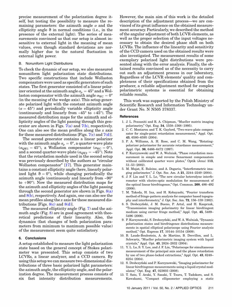
To check the dynamic of our setup, we also measurednonuniform light polarization state distributions.Two specific constructions that include Wollastoncompensatorswere used as specific generators of suchstates. The first generator consisted of a linear polar-izer oriented at the azimuth angle αp ¼ 45° and aWol-laston compensator with the azimuth angle αWC ¼ 0°(in the meaning of the wedge axis). This setup gener-ate polarized light with the constant azimuth angle(α ¼ 45°) and periodically variable ellipticity angle(continuously and linearly from −45° to þ45°). Themeasured distribution maps for the azimuth and el-lipticity angles of the light passing through this gen-erator are shown in Figs. 7(a) and 7(b), respectively.One can also see the mean profiles along the x axisfor these measured distributions [Figs. 7(c) and 7(d)].

The second generator contains a linear polarizerwith the azimuth angle αp ¼ 0°, a quarter-wave plate(αQW1 ¼ 45°), a Wollaston compensator (αWC ¼ 0°),and a second quarter-wave plate (αQW2 ¼ −45°). Notethat the retardation module used in the second setupwas previously described by the authors as “circularWollaston compensator” [17]. This generator main-tains a constant ellipticity angle (here, linearly polar-ized light ϑ ¼ 0°), while changing periodically theazimuth angle (continuously and linearly from −90°to þ90°). Now the measured distribution maps forthe azimuth and ellipticity angles of the light passingthrough the second generator are shown in Figs. 8(a)and 8(b), respectively. And again, one can also see themean profiles along the x axis for thesemeasured dis-tributions [Figs. 8(c) and 8(d)].

The measured ellipticity angle (Fig. 7) and the azi-muth angle (Fig. 8) are in good agreement with theo-retical predictions of their linearity. Also, thedynamics (fast changes of both polarization para-meters from minimum to maximum possible value)of the measurement seem quite satisfactory.

6. Conclusions

A setup established to measure the light polarizationstate based on the general concept of Stokes polari-meter was presented. This setup consists of twoLCVRs, a linear analyzer, and a CCD camera. Byusing this setupwe canmeasure two-dimensional dis-tributions of three basic polarized light parameters:the azimuth angle, the ellipticity angle, and the polar-ization degree. The measurement process consists ofsix fast intensity distribution measurements.

However, the main aim of this work is the detaileddescription of the adjustment process—we are con-vinced of its great influence on the obtainedmeasure-ment accuracy. Particularly, we described the methodof the angular adjustment of both LCVR elements, aswell as the proper selection of the input voltages ne-cessary to obtain the desired phase shift on bothLCVRs. The influence of the linearity and sensitivityof the CCD camera used on the obtained results werealso investigated. The measurement results of someexemplary polarized light distributions were pre-sented along with the error analysis. Finally, the ob-tained results convinced us of the necessity to carryout such an adjustment process in our laboratory,Regardless of the LCVR elements’ quality and com-pleteness of their specifications obtained from theproducer, a reliable adjustment method for complexpolarimetric systems is essential for obtainingreliable results.

This work was supported by the Polish Ministry ofScientific Research and Information Technology un-der Grant No. N N505 378337.

References1. J. L. Pezzaniti and R. A. Chipman, “Mueller matrix imaging

polarimetry,” Opt. Eng. 34, 1558–1568 (1995).2. C. C. Montarou and T. K. Gaylord, “Two-wave-plate compen-

sator for single-point retardation measurement,” Appl. Opt.43, 6580–6595 (2004).

3. P. A. Williams, A. H. Rose, and C. M. Wang, “Rotating-polarizer polarimeter for accurate retardance measurement,”Appl. Opt. 36, 6466–6472 (1997).

4. P. Kurzynowski and W. A. Woźniak, “Phase retardation mea-surement in simple and reverse Senarmont compensatorswithout calibrated quarter wave plates,” Optik (Jena) 113,51–53 (2002).

5. M. Mujat, E. Baleine, and A. Dogariu, “Interferometric ima-ging polarimeter,” J. Opt. Soc. Am. A 21, 2244–2249 (2004).

6. J. F. Lin and Y. L. Lo, “The new circular heterodyne interfe-rometer with electro-optic modulation for measurement ofthe optical linear birefringence,” Opt. Commun. 260, 486–492(2006).

7. M. Takeda, H. Ina, and H. Kobayashi, “Fourier transformmethod of fringe-pattern analysis for computer based topogra-phy and interferometry,” J. Opt. Soc. Am. 72, 156–159 (1982).

8. S. Drobczyński, J. M. Bueno, P. Artal, and H. Kasprzak,“Transmission imaging polarimetry for linear birefringentmedium using carrier fringe method,” Appl. Opt. 45, 5489–5496 (2006).

9. P. Kurzynowski, S. Drobczyński, andW. A.Woźniak, “Dynamicpolarization states and birefringence distributions measure-ments in spatial elliptical polariscope using Fourier analysismethod,” Opt. Express 17, 10144–10154 (2009).

10. B. Laude-Boulesteix, A. de Martino, B. Drevillon, and L.Schwartz, “Mueller polarimetric imaging system with liquidcrystals,” Appl. Opt. 43, 2824–2832 (2004).

11. Y. L. Lo, S. Y. Lee, and J. F. Lin, “Polariscope for simultaneousmeasurement of the principal axis and the phase retardationby use of two phase-locked extractions,” Appl. Opt. 43, 6248–6254 (2004).

12. S. Drobczyński and P. Kurzynowski, “Imaging polarimeter forlinear birefringencemeasurements using a liquid crystal mod-ulator,” Opt. Eng. 47, 023603 (2008).

13. T. Sato, T. Araki, Y. Sasaki, T. Tsuru, T. Tadokoro, and S.Kawakami, “Compact ellipsometer employing a static


polarimeter module with arrayed polarizer and wave-plateselements,” Appl. Opt. 46, 4963–4967 (2007).

14. K. Oka and T. Kaneko, “Compact complete imaging polari-meter using birefringent wedge prisms,” Opt. Express 11,1510–1519 (2003).

15. K. Oka and N. Saito, “Snapshot complete imaging polarimeterusing Savart plates,” Proc. SPIE 6295, 629508 (2006).

16. W. A. Woźniak and P. Kurzynowski, “Compact spatial polari-scope for light polarization state analysis,” Opt. Express 16,10471–10479 (2008).

17. P. A. Williams, “Rotating-wave-plate Stokes polarimeter fordifferential group delay measurements of polarization-modedispersion,” Appl. Opt. 38, 6508–6515 (1999).

18. P. Goudail, P. Terrier, Y. Takakura, L. Bigué, F. Galland, andV. Devlaminck, “Target detection with liquid-crystal-

based passive Stokes polarimeter,” Appl. Opt. 43, 274–282(2004).

19. J. E. Wolfe and R. A. Chipman, “Polarimetric characterizationof liquid-crystal-on-silicon panels,” Appl. Opt. 45, 1688–1703 (2006).

20. J. S. Baba and P. R. Boudreaux, “Wavelength, temperatureand voltage dependent calibration of a nematic liquid crystalmultispectral polarization generating device,” Appl. Opt. 46,5539–5544 (2007).

21. P. Terrier, J. M. Charbois, and V. Devlaminck, “Fast-axis orien-tation dependence on driving voltage for a Stokes polarimeterbased on concrete liquid-crystal variable retarders,” Appl.Opt. 49, 4278–4283 (2010).

22. P. Yeh and C. Gu, “Optics of Liquid Crystal Displays(Wiley, 2010).


Documents

Adjustment method of an imaging Stokes polarimeter based on liquid crystal variable retarders