Additional Notes on 2D Finite Element Method.Math 610:700, Spring 2019

weip@math.tamu.edu

Our task is to numerically solve the second order elliptic problem in twodimensional space using finite element method.

We consider the following model problem: let Ω = (−1, 1)2\[0, 1)2 be theL-shaped domain, we seek u : Ω→ R, such that

(0.1) −∆u+ qu = f in Ω, u = 0 on ∂Ω.

Here the functions q(x) ≥ 0 and f are both given. We can write a weak formulation:find u ∈ H1(Ω) satisfying

(0.2)

∫Ω

(∇u · ∇v + quv) dx =

∫Ω

fv dx, for all v ∈ H10 (Ω).

The approximation scheme consists of developing finite element method to findapproximated solutions to the weak problem (0.2).

1. Triangulation

To start with, we need to discretize the open bounded domain Ω ⊂ R2 intotriangles. The discussion in this section applies to generic domains.

Notations. To simplify our problem, let us assume that our bounded domain Ωis polygonal. Non-polygonal domains such as unit disc requires additional treatmentfor the geometry. We then subdivide Ω (including Ω and the boundary ∂Ω) withmany small closed triangles (quadrilaterals are also allowed, but we will not considerhere). Let us denote T to be the collection of all the triangles. Since Ω is open (notincluding boundary), Ω is equal to interior of the union of all the triangles, i.e.

Ω =(⋃

τ∈T τ)o

. Figure 1 shows a triangular mesh in the square domain (−1, 1)2.

There are two basic rules when we are talking about a mesh for our finiteelement implementation:

a) One triangle cannot overlap any other triangles. This means that if τi and τj aretwo distinct triangles in T, the intersection of their interiors should be empty,i.e. τo

i ∩ τoj = ∅.

b) Given two distinct triangles τi and τj , their intersection τi ∩ τj should be onlyone of the following cases: an empty set ∅, a common vertex or a commonedge. This indicates that the case in Figure 2 is not allowed. In Figure 2, wecall the vertex at the interior of an edge as a hanging node. We say a meshis admissible or conforming if the mesh has no hanging nodes (see Figure 1).Here we remark that we can deal with the hanging nodes using some specialtechniques but it is a bit more complicated (this is in fact quite useful when the

1

2

-1 -0.8 -0.6 -0.4 -0.2 0 0.2 0.4 0.6 0.8 1

-1

-0.8

-0.6

-0.4

-0.2

0

0.2

0.4

0.6

0.8

1

Figure 1. A uniform structured mesh in [−1, 1]2.

element is quadrilateral). For simplicity, we only consider admissible triangularmeshes in our problem.

hanging node

Figure 2. A non-conforming mesh.

Shape regularity . To make sure that we can generate a sequence of meshesso that our approximated solutions on these meshes will convergence to the exactsolution, we need two more requirements on the meshes. The first one is the shaperegularity. For a triangle τ in the mesh T, there exists a smallest circle so thatthe triangle τ is inside this circle (circumcircle), we denote hτ the diameter of suchcircle. Also, there exists a largest circle inscribed in τ (inscribed circle) and wedenote rτ the diameter of the inscribed circle. We say a mesh T is shape-regular

3

provided that there exists a constant c so that

hτrτ≤ c

holds for any triangle τ ∈ T. The constant c is called the shape regularity constantand h = maxτ hτ denotes the size of the mesh.

For a given triangle τ in a mesh T, let θτ be the smallest angle in τ . We canprove that

hτrτ≤ 2

sin θτ.

This inequality implies that if θτ , the smallest angle in τ , is greater than a certainangle θ0 for any triangle τ ∈ T, then the mesh is shape-regular. So roughly speaking,shape-regularity requires all the triangles not to be too “flat”.

Quasi-uniformity . We say a mesh T is quasi-uniform provided that T is shape-regular and there exists a constant ρ so that

ρh ≤ hτ for all τ ∈ T.

This shows that the sizes of any two triangles are similar up to a constant ratio ρ.In a uniform mesh such as the one in Figure 1, we shall observe that ρ = 1. So herewe extend the uniform mesh to a more general setting.

Constructing a mesh. We will solve our 2D problem on shape-regular and quasi-uniform meshes. The first task is to construct a quasi-uniform mesh so that we canuse it in MATLAB. Unfortunately, to our best knowledge, in MATLAB we do not havea direct method to build a mesh that can be controlled by the shape regularity andquasi-uniform constants (e.g. Figure 3).

An alternative software we are going to use is TRIANGLE. The source codeis available at https://www.cs.cmu.edu/˜quake/triangle.html. For a Linux OS ormacOS computer, we can compile the source code in terminal by typing

make all

Remark 1. For mac users, the installation of Xcode, command tools and X11 arerequired. A modification of the makefile from the source code is also necessary. Inline 76, we need to change the SWITCHS flag to

CSWITCHES = -O -DNO_TIMER -I/usr/X11/include -L/usr/X11/lib

After successfully compiling the code, we obtain the executable triangle.The poly-file Lshaped.poly provides the definition of the domain (see here for aninstruction). In terminal, we can generate a L-shaped mesh by using command

./triangle -a.02 -e -q30 Lshaped.poly

Here the parameters

4

-1 -0.8 -0.6 -0.4 -0.2 0 0.2 0.4 0.6 0.8 1

-1

-0.8

-0.6

-0.4

-0.2

0

0.2

0.4

0.6

0.8

1

Figure 3. A quasi-uniform mesh for a L-shaped domain.

• -a.02 means that the area of all the triangles is no larger than 0.02. Wecan control the mesh size h by changing the area.• -e outputs (to an .edge file) a complete list of edges in the triangulation.

In some cases (not in our problem) we need to integrate over edges.• -q30 ensures that the smallest angle of each triangle is no less than 30

degrees. This guarantees the quasi-uniformity of the mesh we generate.

The output contains several files. In our problem we will need three of them:Lshaped.1.node, Lshaped.1.ele and Lshaped.1.edge. We also need the MATLAB

function readmesh.m. It reads the files and store the mesh data into MATLAB. Thefunction can be called as follows:

[n_node,n_ele,node,ele,n_edge,edge,is_node_at_boundary]...

= readmesh(’Lshaped.1.node’,’Lshaped.1.ele’,’Lshaped.1.edge’);

Here the output values n node, n ele, and n edge correspond to the number ofvertices, elements, and edges respectively. node is an n node by 2 matrix storingthe coordinates of all the vertices. ele and edge are lists of triangles and edges.The vector is node at boundary is a boolean vector to check whether each nodein the node list is on the boundary.

For instance, in the first row of ele, 8, 21, 77 gives the triangle with verticesto be the 8th, 21st and 77th nodes in the node list.

The function meshplot.m can plot the continuous piecewise linear function onthe corresponding mesh. For example, suppose that we have read and stored the

5

Figure 4. Interpolation of f(x, y) = sin(πx) + sin(πy) on the L-shaped domain.

mesh described as above into MATLAB, we can plot the interpolation of the functionf(x, y) = sin(πx) + sin(πy) on the mesh by

y = @(x1,x2) sin(pi*x1)+sin(pi*x2);

meshplot(ele,node,y(node(:,1),node(:,2)));

See Figure 4 for an illustration. We can use this function to visualize the approxi-mated solution.

2. Finite element approximation

In this section we first discuss the continuous piecewise linear finite elementspace subordinated in a quasi-uniform mesh.

The finite element space. Given a quasi-uniform and shape-regular mesh Thwith the mesh size h > 0, we denote by Vh the space of the continuous piecewiselinear functions on Th. Namely, for any vh ∈ Vh, the function vh is continuous andits restriction to any triangle τ ∈ Th is a linear function (see e.g. Figure 4). Similarto the 1D case, the finite element basis functions have the following property: givenxi in the node list, the corresponding basis function φi satisfies

φi(xi) = 1, and φi(xj) = 0 for all xj 6= xi.

Figure 5 shows two example basis functions.

6

Figure 5. (Left) A finite element basis function at the boundaryand (Right) a finite element basis function in the interior of thedomain.

The set φi forms a complete basis for the finite element space Vh, thereforeany vh ∈ Vh is a linear combination of φi, that is

vh(x) =

M∑i=1

ciφi(x),

where M is the dimension of Vh.

Reference triangle, affine mapping and local basis functions. Recall that webuild the stiffness matrix in 1D by assembling local stiffness matrices for each subin-terval. In 2D, we follow the same element-by-element approach, thus we need tobuild the local stiffness matrix for every cell (triangle). Since a triangle has threevertices, we shall have three local basis functions. Therefore, the local stiffnessmatrix should be a 3× 3 matrix.

In 1D it was convenient to write the local basis functions and their derivativesdirectly. However, in 2D a direct representation is not readily available, hence wedefine the local basis functions in a different approach.

We define the reference triangle τ with three vertices (0, 0), (1, 0) and (0, 1),see Figure 6. Given any arbitraty triangle τ ∈ Th with three vertices (x1, y1),(x2, y2) and (x3, y3), we can map τ to τ using the mapping(

x

y

)= T (x, y) :=

(x2 − x1 x3 − x1

y2 − y1 y3 − y1

)︸ ︷︷ ︸

=:B

(x

y

)+

(x1

y1

)for (x, y) ∈ τ .

7

Clearly, a sanity check shows that T maps the vertices of τ to the vertices of τ (thatis, (0, 0) 7→ (x1, y1), (1, 0) 7→ (x2, y2), and (0, 1) 7→ (x3, y3)). We can also provethat, if f(x, y) is a linear function in τ , f(T (x, y)) is a linear function in τ . Themapping T is also one-to-one, therefore the inverse mapping T−1 : τ → τ exists.

(0, 0) (1, 0)

(0, 1)

τ

(x1, y1) (x2, y2)

(x3, y3)

τ

(a) (b)

Figure 6. (a) The reference triangle τ and (b) the real arbitrarytriangle τ .

It is not difficult to derive that the local basis functions on τ are

φ1 = 1− x− y, φ2 = x, and φ3 = y.

Their first order derivatives are

∇φ1 = (−1,−1)t, ∇φ2 = (1, 0)t, and ∇φ3 = (0, 1)t.

Here ∇φi denotes the gradient of φi with respect to (x, y).

With the assistance of mapping T−1, the local basis functions on τ can bedefined as

φi(x, y) = φi(T−1(x, y)), for i = 1, 2, 3.

Also, invoking the chain rule, we can compute the gradient of φi by

∇φi = (J(T−1))t∇φi.

Here J(T−1) is the Jacobian of the inverse of T . Since T is a linear mapping,

J(T−1) := B−1 =

(x2 − x1 x3 − x1

y2 − y1 y3 − y1

)−1

.

8

Numerical integration. To compute the entries of the local stiffness matrix onan arbitrary triangle τ ∈ Th,

aτi,j :=

∫τ

a(x, y)∇φi · ∇φj dxdy, for i, j = 1, 2, 3,

we will map the trangle τ to the reference element τ , and apply the numericalintegration on τ . In the first step, by change of the variables using the mapping T ,we have

aτi,j :=

∫τ

a(x, y)∇φi · ∇φj dxdy

=

∫τ

a(T (x, y))[(J(T−1))t∇φi] · [(J(T−1))t∇φj ]|detB| dxdy.

In the second step, given the quadrature points q1, q2, . . . , qk and the quadratureweights w1, w2, . . . , wk for the integral on τ , we define the approximation to theabove integral by∫

τ

a(x, y)∇φi · ∇φj dxdy

≈k∑l=1

wla(T (ql))[(J(T−1))t∇φi(ql)] · [(J(T−1))t∇φj(ql)]|detB|,

for i, j = 1, 2, 3. An example quadrature formula is∫τ

f(x) dx ≈ 1

24(f(0, 0) + f(1, 0) + f(0, 1) + 9f(

1

3,

1

3)).

The above formula is exact for polynomial f ∈ P2.

Remark 2. Another type of commonly used quadrature rule is the Gaussian quad-rature: ∫

τ

f(x, y) dx dy ≈nq∑j=1

wjf(xj , yj).

Table 1 lists the first five quadrature rules. Notice that these rules have the property(can be verified by taking f = 1)

nq∑j=1

wj = 0.5.

Higher orders quadrature rules can be found here.

9

k nq xj yj wj1 1 0.333333333333330 0.333333333333330 1.000000000000000

2 30.166666666666670 0.166666666666670 0.3333333333333300.166666666666670 0.666666666666670 0.3333333333333300.666666666666670 0.166666666666670 0.333333333333330

3 4

0.333333333333330 0.333333333333330 -0.5625000000000000.200000000000000 0.200000000000000 0.5208333333333300.200000000000000 0.600000000000000 0.5208333333333300.600000000000000 0.200000000000000 0.520833333333330

4 6

0.445948490915970 0.445948490915970 0.2233815896780100.445948490915970 0.108103018168070 0.2233815896780100.108103018168070 0.445948490915970 0.2233815896780100.091576213509770 0.091576213509770 0.1099517436553200.091576213509770 0.816847572980460 0.1099517436553200.816847572980460 0.091576213509770 0.109951743655320

5 7

0.333333333333330 0.333333333333330 0.2250000000000000.470142064105110 0.470142064105110 0.1323941527885100.470142064105110 0.059715871789770 0.1323941527885100.059715871789770 0.470142064105110 0.1323941527885100.101286507323460 0.101286507323460 0.1259391805448300.101286507323460 0.797426985353090 0.1259391805448300.797426985353090 0.101286507323460 0.125939180544830

Table 1. Quadrature rules exact for p ∈ Pk(τ) on the standard2D reference triangle τ .

Approximation of local mass matrix . Similarly, we can approximate the localmass matrix and the local right hand side vector by

mτi,j =

∫τ

b(x, y)φiφj dxdy

≈k∑l=1

wlb(T (ql))φi(T (ql))φj(T (ql))|detB|

=

k∑l=1

wlb(T (ql))φi(ql)φj(ql)|detB| for i, j = 1, 2, 3.

10

and

fτi =

∫τ

f(x, y)φi(x, y) dxdy

≈k∑l=1

wlf(T (ql))φi(T (ql))|detB|,

=

k∑l=1

wlf(T (ql))φi(ql)|detB|, for i = 1, 2, 3.

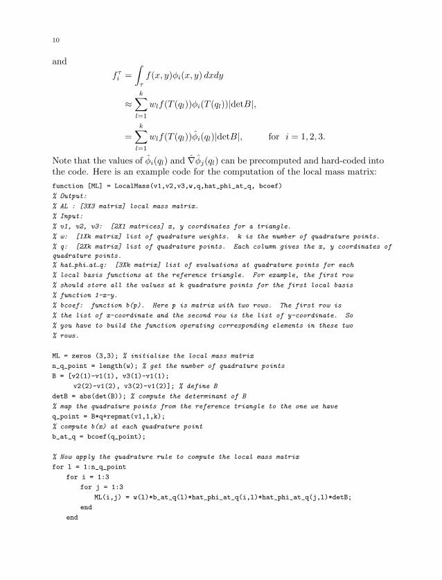
Note that the values of φi(ql) and ∇φj(ql) can be precomputed and hard-coded intothe code. Here is an example code for the computation of the local mass matrix:

function [ML] = LocalMass(v1,v2,v3,w,q,hat_phi_at_q, bcoef)

% Output:

% AL : [3X3 matrix] local mass matrix.

% Input:

% v1, v2, v3: [2X1 matrices] x, y coordinates for a triangle.

% w: [1Xk matrix] list of quadrature weights. k is the number of quadrature points.

% q: [2Xk matrix] list of quadrature points. Each column gives the x, y coordinates of

quadrature points.

% hat phi at q: [3Xk matrix] list of evaluations at quadrature points for each

% local basis functions at the reference triangle. For example, the first row

% should store all the values at k quadrature points for the first local basis

% function 1-x-y.

% bcoef: function b(p). Here p is matrix with two rows. The first row is

% the list of x-coordinate and the second row is the list of y-coordinate. So

% you have to build the function operating corresponding elements in these two

% rows.

ML = zeros (3,3); % initialize the local mass matrix

n_q_point = length(w); % get the number of quadrature points

B = [v2(1)-v1(1), v3(1)-v1(1);

v2(2)-v1(2), v3(2)-v1(2)]; % define B

detB = abs(det(B)); % compute the determinant of B

% map the quadrature points from the reference triangle to the one we have

q_point = B*q+repmat(v1,1,k);

% compute b(x) at each quadrature point

b_at_q = bcoef(q_point);

% Now apply the quadrature rule to compute the local mass matrix

for l = 1:n_q_point

for i = 1:3

for j = 1:3

ML(i,j) = w(l)*b_at_q(l)*hat_phi_at_q(i,l)*hat_phi_at_q(j,l)*detB;

end

end

11

end

end

The computation of local stiffness matrix and local right hand side vector issimilar.

Assembly of global matrices and vectors. The “element-by-element” techniqueis used to assemble the global matrices and rhs vector.

We can either create a single assembly matrices function that assembliesmatrices and rhs at the same time, or we can write separate routines for each. Herewe choose the first approach and write them into the same function.

For notational convenience, we denote Ni to be the number of interior nodes.Same as in the 1D case, the solution at the boundary nodes are already determined- they are fixed to be zero, therefore the global mass matrix M and global stiffnessmatrix A should only include the Ni interior nodes. In the following routine theI full array serves as a boundary/interior indicator.

% set boundary indicator

k = 0;

j = 0;

I_full = zeros(n_nodes, 1);

for m = 1:n_nodes

if (is_node_at_boundary(m))

k = k+1;

boundary(k) = m;

I_full(m) = -k;

else

j = j+1;

interior(j) = m;

I_full(m) = j;

end

end

We now assembly the matrices:

function [A,M] = assembly_matrices(n_ele,eles,nodes,I_full,N_i)

l=0;

for j=1:n_ele

v1 = nodes(eles(j,1),:);

v2 = nodes(eles(j,2),:);

v3 = nodes(eles(j,3),:);

[B, absdB, InvB] = mapping(v1,v2,v3);

ls = localStiff(InvB, absdB);

lm = localMass(absdB);

for m = 1:3

12

if I_full(eles(j,m))>0

for k = 1:3

if I_full(eles(j,k))>0

l = l+1;

ii(l) = I_full(eles(j,m));

jj(l) = I_full(eles(j,k));

v_mass(l) = ls(m,k);

v_stiff(l) = ls(m,k);

end

end

end

end

end

% create the sparse matrices

A = sparse(ii,jj,v_mass,N_i,N_i);

M = sparse(ii,jj,v_stiff,N_i,N_i);

end

Solve the linear system. Recall that the system matrix S (in this example,S = A + M) is assembled as a sparse matrix. We shall solve the linear equationsystem using the backslash solver to obtain the solution vector

sol interior = S\F.

Note that the solution vector has values on the Ni interior nodes only. We need tomap back to the full vector. This is done by using the interior array:

sol = zeros(n_nodes,1); % all boundary nodes have value 0

for j = 1:n_interior

sol(interior(j)) = sol_interior(j);

end

Solution visualization. MATLAB has a convenient function trimesh that readilyplots the solution associated to the triangulation. The inputs are the element array,the node array, and the solution array:

trimesh (eles, nodes(:,1), nodes(:,2), sol);

Errors. The L2 and H1 error computations follow the same procedure as inthe 1D case, i.e. collecting the local error at each element using the quadratureformula.

Remark 3. For non-homogeneous Dirichlet boundary conditions, extra proceduresare required for the right hand side vector; refer to Homework 8.

13

3. Appendix: A python code for finite elements

The reason for writing this Python program is two fold. On one hand, Pythonis nowadays a popular programming language, and it is easy to learn, fully featuredfor scientific computation, and includes strong science libraries such as NumPy. Onthe other hand, the university has stopped providing free MATLAB student license,which is making the open-source Python programming more favorable. When com-pared with MATLAB, the generic logic in python is the same, but the syntax isdifferent. Here is a simple comparison between Python and MATLAB.

The Python installation package is available here. You also need the NumPypackage.

After downloading my Python code, you may unzip it, navigate to the direc-tory in terminal, and run the code by typing

python FEMdriver.py

You shall see the error table printed in terminal, as well as the plots for solutionsand error convergence rates. Figures 7 and 8 are the solutions to Problem 1 ofhomework 8.

Have fun!

(a) (b)

Figure 7. The errors to Problem 1 of homework 8. (a) the printederrors in terminal; (b) the log-log plot.

14

(a) (b)

(c) (d)

Figure 8. The solution to Problem 1 of homework 8. (a) thecoarsest mesh, (d) the finest mesh.