Embed Size (px)
Citation preview

ADAPTIVE TRAFFIC CONTROL SYSTEM
DESIGN AND SIMULATION
Duy Nhat Nguyen
A thesis
in
The Department
of
Computer Science and Software Engineering
Presented in Partial Fulfillment of the Requirements
For the Degree of Master of Computer Science
Concordia University
Montreal Quebec Canada
July 2015
c⃝ Duy Nhat Nguyen 2015
Concordia UniversitySchool of Graduate Studies
This is to certify that the thesis prepared
By Duy Nhat Nguyen
Entitled Adaptive Traffic Control System Design and Simulation
and submitted in partial fulfillment of the requirements for the degree of
Master of Computer Science
complies with the regulations of this University and meets the accepted standards with
respect to originality and quality
Signed by the final examining commitee
ChairDr Sabine Bergler
ExaminerDr Sudhir Mudur
ExaminerDr Joey Paquet
SupervisorDr Vangalur Alagar
ApprovedChair of Department or Graduate Program Director
20
Faculty of Engineering and Computer Science
Abstract
Adaptive Traffic Control System Design and Simulation
Duy Nhat Nguyen
Traditional traffic control infrastructures have not changed much in the last several decades
while the volume of traffic has increased disproportionably to infrastructure improvement
A solution to mobility cannot be addressed by simply improving the technology of a single
vehicle any further A solution is to enable people to reach their destinations safely and in
optimal time given the topology of road networks This thesis offers such a solution based on
an adaptive traffic control algorithm which takes the road network topology and dynamically
varying traffic streams as input and guarantees dependable and optimal mobility for vehicles
The algorithm calculates dependable passages for vehicles to cross road intersections and
enables point-to-point travel by minimizing travel time and maximizing fuel consumption
The adaptive algorithm is embedded in the Arbiter managed by an Intersection Manager
at every road intersection A distributed traffic management architecture consisting of a
hierarchy of road managers is proposed in the thesis Extensions to the adaptive algorithm
and the architecture are given The extended algorithm will efficiently function under
exceptional situations such as bad weather road repairs and emergency vehicle mobility
The extended architecture is expected to have autonomic computing properties such as
self-healing self-recovery and self-protection and Cyber-physical system properties such as
tightly-coupled feed-back loops with all entities in its environment A simulator has been
implemented and simulated results reveal that the adaptive algorithm is far superior in
performance to fixed-time control systems
iii
Acknowledgments
I would like to express my kindest gratitude to my supervisor Professor Vangalur Alagar for
his support his guidance and especially his trust and respect to me During the last two
years he has been working extremely hard with me to solve all problems that we encountered
It is a privilege to know him to work with him and to be his student In him I learned not
only from his profound knowledge but also from his great personality
This work is also dedicated to my parents my sisters my brothers and especially to my wife
who always encouraged me throughout the work
iv
Contents
List of Figures ix
List of Tables xi
1 Introduction 1
11 Basic Concepts of TDM 3
111 Control Variables 3
112 Signal Parameters for Traffic at an Intersection 7
12 Contributions and Outline of Thesis 11
2 Related Works 13
21 Traffic Control Strategies 14
22 A Review of Existing Traffic Control Strategies 15
221 SIGSET 15
222 TRANSYT 16
223 SCOOT 17
224 RHODES 19
225 Summary and Comparison 22
3 Architectural Design 23
31 Objectives of ATCS 24
311 Dependability Objectives Safety Liveness and Fairness 24
312 Optimization Objectives 25
32 Architecture 26
v
321 Traffic Detector 26
322 Flow Builders 28
323 Traffic Actuator 30
324 Controller 30
325 Arbiter 31
326 Context Manager 32
327 Intersection Manager 33
328 Zone Manager 34
4 Arbiter - Algorithm Design 35
41 Intersection Structure 36
411 Inbound Queue 36
412 Waiting Queue 37
413 Linkage Lane 38
42 Clique 40
421 Constructing a Set of Cliques 41
422 Example of Clique 42
43 Vehicle Score 43
431 Route Score 43
432 Aging Function 45
433 Definition of Vehicle Score s(t) 46
44 Rolling Horizon Streams(RHS) 47
441 Rolling Flows 48
442 Ranking Clique 49
443 Deactivating Non-member Lanes 50
444 Activating Member Lanes 52
445 Update Interval 54
45 Extended RHS 54
451 Emergency Vehicles 54
452 Pedestrians 55
vi
46 Integrating Context Parameters in RHS 56
47 Correctness and Complexity of RHS 58
471 Correctness of RHS 59
472 Complexity of RHS 60
5 Road Network Topology 62
51 Overview 62
52 Road Network Description 63
521 Node in RND 63
522 Road in RND 63
523 Lane in RND 65
524 Intersection in RND 65
525 Road Network Description Model Example 65
53 Road Network Topology 66
531 Node in RNT 66
532 Road in RNT 68
533 Lane in RNT 68
534 Lane Segment in RNT 68
535 Shape in RNT 69
536 Intersection in RNT 69
537 Linkage in RNT 69
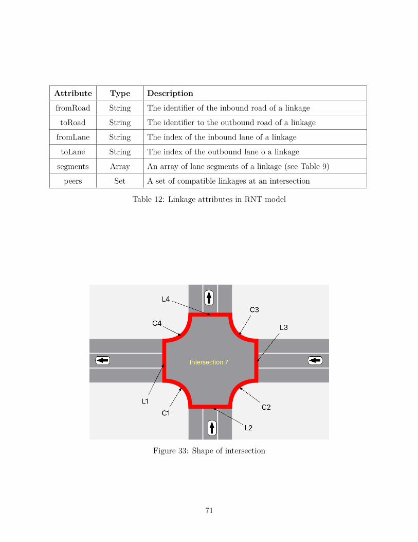
54 Shape of an intersection 70
6 Vehicle Driver Behavior 72
61 Car Following Models 72
611 Elements of Car Following Models 73
612 Gippsrsquo Model 74
613 Intelligent Driver Model 77
614 Special Situations 79
62 Lane Changing 79
621 Improved Model of SITRAS 80
vii
622 Following Graph 85
7 Implementation 88
71 Toolchain 88
711 Preprocessing Stage 89
712 Operating 89
713 Analyzing 90
72 Features 91
721 Nondeterministic 91
722 Scalable System 92
73 Simulation Results 92
731 Mean Speed 93
732 Low Traveling Speed Ratio (LTSR) 93
733 Congestion Rate 95
734 Fuel Consumption 96
8 Conclusions and Future Work 99
81 Contributions 99
82 Limitations 102
83 Future Work 104
831 Formal Verification 104
832 Architectural Extensions for Supporting Transportation Cyber Physical
System 105
Bibliography 109
viii
List of Figures
1 Headway Gap and Vehicle Length 4
2 Relation between Flow Rate and Density [1] 6
3 Partial-conflict phases 7
4 Platoon of Vehicles 8
5 Green wave occurs when vehicle crossing intersections 10
6 Time distance and green phase coordination in Green wave 10
7 Outline of Thesis 12
8 How SCOOT works [47] 18
9 The RHODES hierarchical architecture [34] 20
10 How RHODES works 21
11 Hierarchy of ATCS 23
12 Conceptual Architecture of ATCS 27
13 Pedestrian detector using video image processor [22] 28
14 V2V and V2I Communication 29
15 Feedback loop at an intersection 32
16 Factors determining traffic policy 33
17 Queues at an intersection 36
18 Linkages and turn restriction 39
19 Single Lane Intersection 40
20 Set of cliques at an intersection 42
21 Routes at an intersection 43
22 Aging function g = t2900 + 1 47
23 Four steps of RHS 48
ix
24 Flowchart of deactivating non-member lanes 51
25 Detecting wasted Time 52
26 Flowchart of activating member lanes 53
27 Cliques in the extended RHS 56
28 Converting to RNT from RND and OSM 63
29 Lane Index 65
30 RND Model Example 67
31 Road Network of Figure 30 67
32 Internal structure of Intersection 7 of Road Network in Figure 31 70
33 Shape of intersection 71
34 Main steps of Car Following models 73
35 Notations of Car Following models 74
36 Flowchart of Lane Changing 81
37 Notations for Gap Acceptance 82
38 Collision when two vehicles performing lane changes 83
39 Path of vehicle when performing lane change 84
40 Forced lane changing model 85
41 Deadlock in forced lane changing 85
42 Following Graph of Figure 41 87
43 Toolchain of CMTSim 89
44 Snapshot of Viewer on OSX 91
45 Simulation Result - Mean Speed 94
46 Congestions occur at multiple intersections 103
x
List of Tables
1 Notable traffic control systems 15
2 Comparison between ATCS and notable traffic control systems 22
3 Influences of the context parameters to RHS 57
4 Node attributes in RND model 63
5 Road attributes in RND model 64
6 Lane attributes in RND model 65
7 Node attributes in RNT model 66
8 Road attributes in RNT model 68
9 Lane attributes in RNT model 68
10 Lane segment attributes in RNT model 69
11 Intersection attributes in RNT model 70
12 Linkage attributes in RNT model 71
13 Set of utilities of CTMSim 90
14 Simulation Result - Mean Speed 95
15 Simulation Result - Low Traveling Speed Ratio 96
16 Simulation Result - Congestion Rate 97
xi
Chapter 1
Introduction
For more than a century automobile and other motorized vehicles have been used to efficiently
transport people and products across a network of roads in the world The demands for
mobility have been increasing ever since urbanization happened after the industrial revolution
In modern times the technology used to develop vehicles which was mainly based on the
laws of mechanics and chemistry has become more sophisticated because of the embedding
of electronic components and automated control systems However the topology of road
networks and their infrastructure for regulating the traffic of modern day vehicles has not
improved in most of the large urban areas in the world Thus the original traditional
traffic control infrastructures are becoming awfully inadequate to handle the modern-day
vehicular traffic which can be characterized by density of vehicles speed of individual vehicles
timeliness constraints of human drivers and the traffic regulation policies laid down by urban
administrators In reality these aspects are not well coordinated Consequently traffic
congestion occurs frequently in large metropolitan cities even in developed countries such
as United States Canada and in many countries in Europe INRIX [29] reports that in
2013 traffic congestion has cost Americans $124 billion in direct and indirect losses and
this amount is estimated to rise 50 percent by 2030 The cumulative loss over the 17-year
period from 2014 to 2030 will be $28 trillion which roughly equals the taxes paid in USA
in 2013 Traffic congestion not only damages the lifeline of the economy but also increases
environmental pollution It is estimated [10] that in 2004 transportation congestion would
contribute approximately 33 of carbon dioxide emissions in the United States which will
1
create serious health and safety problems Thus congestion avoidance is an absolute necessity
for improving urban traffic system It is needed now more than ever It is in this context this
thesis makes a significant contribution
City planners and researchers have proposed two kinds of solutions to reduce traffic
congestion One solution is expanding road infrastructure and another solution is optimizing
Traffic Control System(TCS) The first solution is either inapplicable in many cities due to
physical constraints or unaffordable in many places due to its huge cost overhead Moreover
a simple extension of existing physical network of roads and their infrastructures will not yield
optimal results unless sophisticated control algorithms are embedded in TCS So the second
solution has been preferred by urban planners and actively researched recently However
most of the current TCSs have many drawbacks These include the following
1 They are not reactive to traffic flow and adaptive to dynamic changes in the traf-
fic Consequently there is no fairness in traffic distribution especially across road
intersections
2 In general current TCS design favors vehicular traffic with little consideration for
pedestrian mobility Consequently pedestrians might get frustrated and indulge in
unsafe behavior [36]
3 Control mechanisms in current TCSs neither use context information nor driven by
traffic control policies
4 Feedback loop that is necessary to factor the dynamic changes in traffic flow is absent
in most of current traffic control systems
This thesis is a contribution to the development of a new resilient traffic control system in
which (1) traffic control policies governing pedestrian mobility and vehicular traffic will be
enforced equitably in order to optimize the overall flow of vehicular and human traffic (2)
dynamic feedback loop will be realized at every road intersection and (3) context-dependent
policies will be used to regulate traffic flow The TCS thus realized in this thesis is called
Adaptive Traffic Control System (ATCS) The ATCS design and algorithmic features have
been chosen in a judicious manner with the grand vision that the ATCS can be easily
2
extended and deployed in any future development of a dependable Transportation Cyber
Physical System which will enable vehicle-to-infrastructure (V2I) vehicle-to-vehicle (V2V)
cyber communications and advanced assistance to driverless vehicles
In order to identify a set of requirements and craft a design for ATCS it is necessary to
understand the basic concepts related to Transportation Domain (TDM) and these are given
next
11 Basic Concepts of TDM
Basic concepts of traffic system and traffic control system are explained in this section These
concepts taken from TDM were defined and used by many traffic experts and researchers
for decades
111 Control Variables
Some of the common control variables [1] that are used to estimate and evaluate the
characteristics of traffic conditions are explained below These are essentially the input
parameters that ATCS will need for making traffic control decisions both on a road as well
as at any intersection
Vehicle Presence
Vehicle Presence is a boolean variable that indicates the presence or absence of a vehicle at
a certain point in a roadway The presence of vehicle is detected through sensors such as
induction loop or camera
Flow rate
Flow rate Q is number of vehicles N passing through a specific point on a roadway during a
time period T It is defined as
Q = NT (1)
3
Occupancy
Occupancy is defined as the percentage of time that a specific point on the road is occupied
by a vehicle
Traffic Flow Speed
In traffic management speed of traffic flow is defined as average speeds of the sampling of
vehicles either over a period of time or over space
bull Time mean speed is an average of speeds of vehicles passing a specific point on
roadway over a period of time
Vt = 1N
Nsumi=1
vn (2)
where N is a total number of vehicles passing vn is the speed of vehicle n when passing
bull Space mean speed is a harmonic mean of speeds of vehicles passing a roadway
segment
Vs = NNsum
i=1(1vn)
(3)
where N is a total number of vehicles passing segment of road vn is the speed of vehicle
n when passing
Headway
Figure 1 depicts a headway which is measured at any instant as the distance between the
fronts of two consecutive vehicles in the same lane on a roadway
Figure 1 Headway Gap and Vehicle Length
4
Queue Length
Queue Length is the number of vehicles that are waiting to cross an intersection on a specific
lane on a roadway
Flow Rate amp Capacity
Flow Rate (throughput) is defined as the number of vehicles able to cross a specific point on
a roadway during a given time period Capacity is essentially synonymous to the maximum
throughput
Density
Density K is defined as the number of vehicles per unit distance
Q = K times Vs (4)
where K is the density Q is the volume of traffic flow (measured as number of vehicles
hour) and Vs is space-mean speed (measured in km hour) In practice density K can be
computed by the following equation
K =( 1
T
) Nsumi=1
( 1vi
)(5)
where N is the number of vehicles detected during time T vi is the speed of ith vehicle
crossing a detector in a lane and K is the density of detected lane
Fundamental diagram of traffic flow
Figure 2 is the fundamental diagram of traffic flow which illustrates the relation between flow
rate and traffic density The relation is changed over four different ranges of value of density
These ranges are outlined as below
1 0 le k lt kc
When density is less than the critical density(kc) flow rate increases monotonically over
5
Figure 2 Relation between Flow Rate and Density [1]
density In this range vehicles can travel with the free-flow speed vf (without braking)
which principally equals to the desired speed
2 k = kc
When density reaches the critical density(kc) flow rate also reaches the peak or the
maximum value of flow rate Vehicles are still able to travel with the free-flow speed vf
3 kc lt kc lt kj
When density is greater than the critical density both flow rate and the speed of flow
decrease Vehicles in the network are no longer to drive with the free-flow speed vf but
with a wave speed vw which is lower than vf
4 kc = kj
When density reaches to the jam density (kj) both flow rate and speed of the flow
reach to zero In other words traffic jam happens when density reaches to the jam
density value
6
112 Signal Parameters for Traffic at an Intersection
Phase
Phase is a set of combination of movements or scenarios at an intersection in which vehicles
and pedestrians can cross without conflict Some traffic control systems allow partial-conflict
movements Figure 3 shows an intersection with two partial-conflict phases
Figure 3 Partial-conflict phases
Cycle Length
Cycle Length is total length of time taken by a traffic light to repeat a complete sequence of
phases at an intersection In many modern traffic control systems some phases are either
skipped or repeated That is cycles are never formed An adaptive traffic control system
may not exhibit cyclic behavior
Split
Split is the amount of lsquogreen timersquo that a traffic control system allocates to a specific phase
during one cycle in order that vehicles and pedestrians may cross an intersection
7
Offset
Offset is green phase difference between consecutive intersections
Platoon Dispersion
A group of vehicles that travel together (as a group) is called a lsquoPlatoon of Vehiclesrsquo Platoon
Dispersion Model is employed in some traffic control systems to estimate the traffic flow
profile at a downstream based on the traffic flow that detected at its upstream The behavior
and pattern of a platoon of vehicles are identified according to the following parameters
bull Total number of vehicles in a platoon
bull The average headway of all vehicles in the same platoon
bull The average speed of vehicles in the same platoon
bull Inter-headway which is defined as headway between the last vehicle and the first vehicle
of two consecutive platoons
Platoon Dispersion phenomenon happens when vehicles are moving together as a group
from upstream to downstream and then lsquodispersersquo or spread out because of parking need
difference in speeds or lane changing The primary purpose of studying of platoons is to
estimate the arrival time of a platoon at an intersection in advance which can potentially
increase the ability to optimize the traffic flow along arterial roads
Figure 4 Platoon of Vehicles
8
Lost Time
Lost Time is the duration of non-utilization or unused time within the total time allocated
by the traffic control system for vehicles or pedestrians to cross an intersection There are
three scenarios
bull Scenario 1 Two kinds of lost time occurs when phases are being switched from red to
green or from green to red
ndash Switch from Green to Red Lost time occurs when remaining time is too short
for vehicles or pedestrians to fully cross the intersection When a vehicle or a
pedestrian starts to cross or in the middle of crossing an intersection it may be
that the remaining time for the light to turn red is too short Hence for safety
reason the vehicle or pedestrian will decide not to cross the intersection
ndash Switch from Red to Green Lost time occurs when vehicles are waiting at a red
phase When the traffic light switches to green vehicles have to start up or increase
its speed During the first few moments no vehicles is crossing
bull Scenario 2 Lost time occurs when the traffic control system allocates green time to a
lane but no vehicle is on that lane
bull Scenario 3 Lost time occurs when the traffic control system allocates green time to
a combination of movements but the system allows partial conflict movement such
as allowing left turn Therefore vehicles from two lanes are attempting to cross each
other at the same time using the same intersection space at the intersection In this
scenario the drivers of the two vehicles have to agree on a protocol to solve the conflict
This delay is considered as lost time which reduces the intersection capacity Figure 3
illustrates an intersection with two partial-conflict phases which can lead to Scenario 3
In summary lost time is the primary reason for the capacity at an intersection to be reduced
and the total delay time at an intersection to be increased
9
Figure 5 Green wave occurs when vehicle crossing intersections
Green Wave
Green wave is a coordination mechanism that traffic control systems at multiple intersections
use to synchronize lsquogreen timesrsquo to allow a platoon of vehicles traveling continuously and
smoothly without stopping which can reduce lost time in lsquoScenario 1rsquo The sequence of
movements in Figure5 illustrates how green wave occurs when the vehicle is moving from the
intersection 1 to intersection 4 Figure 6 depicts the time distance and phase coordination of
this sequence of moves
Figure 6 Time distance and green phase coordination in Green wave
10
12 Contributions and Outline of Thesis
The thesis introduces a hierarchical architecture of traffic managers for regulating traffic
flow along roads and intersections of roads At each intersection a feed-back control system
enforces the safe passage of vehicles across the intersection The control system at an
intersection is managed by the Intersection Manager at the intersection The behavior of the
feed-back controller at an intersection is supported by formal mathematical models and the
context-dependent traffic policies enforced by the Intersection Manager at that intersection
Collectively the controllers and Intersection Managers at the intersections in an urban area
fulfill the dependability and optimization properties stated in Chapter 3 The thesis includes
an implementation of the ATCS and its simulation The rest of the thesis in seven chapters
describes the details regarding these results and a comparison with related works The
contributions are organized as follows
The flowchart in Figure 7 depicts the organization of thesis contributions and how they
are related to each other Chapter 2 reviews the traditional traffic control strategies and
the current operational systems based on them The discussion on related work is restricted
to only those works that deal with urban traffic management A conceptual architectural
design of ATCS is given in Chapter 3 The set of dependability and optimization properties
to be realized through the detailed design based on this architecture are stated The roles
of the architectural elements are described to suggest how the satisfaction of the stated
objectives in the architecture is met by their collective behaviors Chapter 4 gives a detailed
discussion on the design of Arbiter which is the central piece of ATCS for an intersection
The rationale for choosing its parameters are stated and supported by formal mathematical
models studied by transportation domain experts The new features in the Arbiter design
are (1) the concept of cliques and collision-free traffic flow discharge algorithm based on it
(2) the definition of vehicle scores and aging function which are crucial design decisions that
facilitate fairness and liveness and (3) the Rolling Horizon Streams (RHS) algorithm which
adapts dynamically to changes in the traffic streams An analysis of the algorithm is given
to assert its satisfaction of the dependability and optimization objectives and establish its
polynomial-time complexity Chapter 5 describes a presentation model for road networks
11
Figure 7 Outline of Thesis
and the preprocessing of network topology descriptions Transformation tools necessary for
the preprocessing tasks have been implemented Chapter 6 discusses a Vehicle Behavior
Model which is necessary to simulate the Arbiter algorithm Without such a model the traffic
scenario necessary for Arbiter control cannot be realistic Chapter 7 describes the simulator
functionalities and shows the simulation results on many data sets Each dataset is created
by combining different demand rates and road network topologies The simulated results
are compared on four criteria chosen as measures to reflect the optimization properties
Chapter 8 concludes the thesis with a summary of contributions their significance and future
work related to the contributions
12
Chapter 2
Related Works
The current research trend pertaining to the development of Intelligent Transportation
Systems(ITS) can be roughly classified into ldquodriverless vehiclesrdquo ldquovehicles with human
driversrdquo and ldquoa hybrid of bothrdquo Research in the first kind focuses in creating autonomous
vehicles (AVs also called automated or self-driving vehicles) that can drive themselves on
existing roads and can navigate many types of roadways and environmental contexts with
almost no direct human input Research in the third kind exploits wireless access for vehicular
environments (WAVE) in order to enable vehicles exchange information with other vehicles on
the road (called V2V) or exchange information with infrastructure mediums (called V2I) such
as RSUs (Road Side Units) AV V2V and V2I rely on continuous broadcast of self-information
by all vehicles (or RSUs) which allows each vehicle to track all its neighboring cars in real
time The degree of precision synchrony and control vary across these three systems The
most pressing challenge in such systems is to maintain acceptable tracking accuracy in
real-time while overcoming communication congestion (and failures) The acceptance of these
technologies by policy makers the inherent complexity in proving the safety and predictability
and the cost of integrating WAVE in vehicles are some of the major impediments in realizing
the dream of either driverless or hybrid systems on the road In this thesis the focus is
on maximizing the infrastructure facilities to minimize traffic congestion for ldquovehicles with
human driversrdquo The TCS that is engineered in this thesis is expected to increase throughput
optimize human safety enhance environmental sustainability and improve human pleasure in
driving So the discussion in this chapter is restricted to the current strategies and systems
13
that are in use with respect to vehicles with drivers
21 Traffic Control Strategies
Current traffic control systems that regulate traffic can be classified into the three categories
Fixed-time Traffic-responsive and Traffic-adaptive [41]
bull Fixed-time
Fixed-time strategy defines a set of traffic control parameters for each intersection for
each period during a day such as morning peak noon or midnight These control
parameters usually are determined after a statistical analysis of traffic flow patterns
The primary drawback of this strategy is its assumption that the traffic demand will be
constant during a period of time such as an hour or 30 minutes
bull Traffic-responsive
Like Fixed-time strategy Traffic-responsive strategy explicitly defines values of control
parameters such as Cycle Split and Offset However instead of using historical traffic
data this strategy uses real-time traffic data obtained from sensors Thus the control
parameters remain valid over a short period in horizon
bull Traffic-adaptive
Unlike Fixed-time and Traffic-responsive Traffic-adaptive strategy does not use Cycle
Split and Offset Instead this strategy selects phase and its green time according to
the real-time traffic data received from the sensors The task of selecting traffic phase
and its green time is called decision which can be implemented by an Optimization
Approach such as Dynamic Programming or Stochastic Programming
In general a traffic control system can regulate a traffic flow at an intersection with or
without coordination with its adjacent intersections An Isolated-Intersection system solely
uses its own traffic data gathered at its intersection to regulate traffic flow at its intersection
Coordinated-Intersection system at an intersection cooperates with the traffic regulators at
its adjacent intersections and make traffic control decisions at its intersection With the
availability of traffic data from the traffic regulators at its adjacent intersections the traffic
14
control system can support Green wave or Oversaturated situations Our proposed system
supports both green wave and oversaturated situation
22 A Review of Existing Traffic Control Strategies
This section briefly reviews some notable traffic control systems which have received attention
from town planners and researchers These are listed in Table 1
System Strategy
SIGSET Fixed-time
TRANSYT Fixed-time
SCOOT Traffic-Responsive
RHODES Traffic-Adaptive
Table 1 Notable traffic control systems
221 SIGSET
SIGSET is a traffic analysis software which was proposed in 1971 by Allsop [6] The primary
purpose of the tool is to generate a set of control parameters for an intersection in a road
network The approach is a well-known example of isolated and fixed-time traffic control
system The input to the tool consists of an intersection E with m phases a set of values di
(1 le i le n) denoting demand at each phase and total lost time for each cycle λ0 These input
values are determined in advance through experiments The output of the system consists of
the length of the traffic light cycle L and a set of split values λi (1 le i le n) for phases which
minimize the total waiting time of vehicles at the intersection Formally
λ0 + λ1 + middot middot middot + λm = L (6)
sj
msumi=1
αijλi ge dj forallj (7)
15
Where λ0 is the total lost time per cycle length λi is split or amount of green time for phase
i L is the cycle length j is a link at the intersection aij = 1 if link j has right of way in
phase i otherwise aij = 0 and dj is the demand at link j of the intersection
222 TRANSYT
TRANSYT (Traffic Network Study Tool) is a traffic simulation and analysis software which
was developed in 1968 by Robertson of the UK Transport and Road Research Laboratory
(TRRL) [44] Currently two main versions of TRANSYT are being researched and developed
in United Kingdom and United States In United States McTrans Center of University of
Florida has released the latest of version TRANSYT-7F for Federal Highway Administration
(FHWA) The primary purpose of TRANSYT is to help town planners or traffic experts
to analysis traffic network and define a set of optimal control parameters for intersections
inside a road network Theoretically the TRANSYT control mechanism is based on lsquoPlatoon
Dispersion Modelrsquo which also was originally developed by Robertson [20] Formally
qprimet+T = F times qt + [(1 minus F ) times qprime(t+T minus1)] (8)
where qprimet+T is the ldquoPredicted flow raterdquo in time interval (t + T ) of the predicted platoon qt is
the ldquoFlow raterdquo of the interval platoon during interval t T is 08times ldquothe cruise travel time on
the linkrdquo and F is ldquosmoothing factorrdquo defined below In the equation below α is ldquoPlatoon
Dispersion Factor (PDF)rdquo selected by traffic experts
F = 11 + αT
(9)
The TRANSYT control mechanism works in an iterative manner [41] First the lsquoinitial
policyrsquo will be loaded into the system and that policy will be used for the next traffic light
cycle For each interval t the system will estimate the traffic flow profile at stop line by
Platoon Dispersion Model then will calculate a Performance Index (PI) in monetary terms
(based primarily on delays and stops) An optimization algorithms such as lsquoHill Climbrsquo [44] or
lsquoSimulated Annealingrsquo [44] will be selected to find optimal control parameters which minimizes
16
Performance Index but respects to defined constraints The new optimal control parameters
will be applied into the next cycle Over time the optimal traffic control parameters will be
generated and these values can be used in real traffic control system Over-saturation is not
included in the first versions but added in the recent versions
Both SIGSET amp TRANSYT work on historical data instead of real-time data and assume
that demand on each link is a constant during a period of time However this assumption is
not accurate in real traffic systems Because the policies selected by both strategies may not
be appropriate for certain periods of time traffic congestion might result in the road network
or traffic capacity may be reduced
223 SCOOT
SCOOT (Split Cycle Offset Optimization Technique) [41] is considered to be a traffic-responsive
version of TRANSYT SCOOT was also developed by Robertson of the UK Transport and
Road Research Laboratory (TRRL) Currently more than 200 SCOOT systems are being
used in more than 150 cities [47] all over the world including London Southampton Toronto
Beijing and Sao Paulo The mechanism of SCOOT is very similar to TRANSYT as both
are based on lsquoPlatoon Dispersion Modelrsquo to estimate the lsquoCycle flow profilesrsquo in advance
The main difference is that SCOOT obtains real-time traffic data through detectors to build
lsquoCycle flow profilesrsquo whereas in TRANSYT historical data is used
Figure 8 illustrates the SCOOT mechanism When vehicles pass through a detector
SCOOT system continuously synthesizes this information to current state of system and
builds platoon of vehicles Based on this it predicts the state of signal as the platoon arrives
at the next traffic light With this prediction the system will try to optimize the signal
control parameters to minimize the lost time at intersections and reduce number of stops and
delays by synchronizing sets of signals between adjacent intersections Three key optimizers
will be executed in SCOOT system These are explained below
1 Split Optimizer
For each phase at every intersection the split optimizer is executed several seconds
17
Figure 8 How SCOOT works [47]
before switching phase from green to red The traffic controller will decide independently
from other intersection controllers whether to switch phase earlier or later or as due
The purpose of this optimization is to minimize the maximization degree of saturation
flow at all approaches of an intersection In order to avoid large change amount of
changed time must be small In practice the value is in the range [-4+4] seconds
2 Offset Optimizer
For each cycle at every intersection the offset optimizer is executed several seconds
before a cycle completes The traffic controller will decide either to keep or alter the
18
scheduled phases at that intersection The output of this decision will affect offset
values between that intersection and its adjacent intersections The purpose of this
optimization is to minimize the sum of Performance Index on all adjacent roads with
offset as scheduled or earlier or later Like the split optimizer the amount of change
time must be small to avoid a sudden transition
3 Cycle optimizer
For 2 - 5 minutes the SCOOT system will make a cycle optimizer at a region (global)
level which consists of many intersections First the SCOOT identifies the critical
nodes whose saturation levels are over the defined threshold (usually 80) then adjusts
the cycle time for those intersections Like previous types of optimizer the cycle time
will be adjusted with small change
Although the system is very successful and being used by many cities SCOOT system
has received many criticisms According to the BBC News Report [36] data pertaining to
pedestrian traffic do not have any real effect on SCOOT controller Pedestrians in cities
where SCOOT is being used call the pedestrian signal button as lsquoPlacebo buttonsrsquo The
problem can be that the SCOOT mechanism gives more importance to vehicular traffic than
pedestrian traffic Another issue of SCOOT is its centralized architecture All optimizations
will be processed at a central computer Consequently there is a single point of failure and
no support for load balance
224 RHODES
RHODES [35] (Real-Time Hierarchical Optimized Distributed Effective System) is a typical
example of traffic-adaptive control which does not have explicit values of control parameters
(see Section 11) such as Cycle Split and Offset Only Phase is defined explicitly In general
the RHODES system consists of two main processes One process called Decision Process
(DP) builds a current and horizon traffic profile based on traffic data from detectors and
other sources Another process called Estimation Process (EP) produces a sequence of
phases and their lengths continuously over the time according to the traffic profile of the
previous process Both DP and EP are situated at three aggregation levels of RHODES
19
hierarchy as shown in Figure 9
Figure 9 The RHODES hierarchical architecture [34]
1 Dynamic Network Loading
Dynamic Network Loading is the highest level in system hierarchy which continuously
and slowly captures macroscopic information of the current traffic Based on this
information it estimates a load or demand on each particular road segment for each
direction in terms of the number of vehicle per hour With these estimates RHODES
system can allocate green times for phases in advance for each intersection in the
network
2 Network Flow Control
Network Flow Control is the middle level in system hierarchy It combines the estimated
result received from the higher level with current traffic flow in terms of platoon or
individual vehicle to optimize the movement of platoon or vehicle individually Figure
10 illustrates how the mechanism of this layer works In Figure 10a it is predicted that
4 platoons may arrive at the same intersection and request to cross These requests
create some conflict movements The RHODES will solve the conflicts by making a
20
tree-based decision on the predicted movement of platoons over horizon as in Figure
10b
(a) Platoons request conflict movements (b) RHODESrsquos decision tree
Figure 10 How RHODES works
3 Intersection Control
Intersection Control is the lowest level in the system hierarchy At this level the system
is dealing with each vehicle at microscopic level Based on the presence of a vehicle
in each lane and decisions communicated by Dynamic Network Loading and Network
Flow Control the Intersection Control uses a Dynamic Programming [34] algorithm to
select phase and assign length of time for that phase
Although Dynamic Programming helps RHODES system to optimize traffic flow by
minimizing average delay and number of stops and maximizing network throughput Dynamic
Programming has its own limitations in optimizing real-time traffic flow problem Powell
explains the ldquoThree Curses of Dimensionality of Dynamic Programmingrdquo [43] of which
computation demand of Bellmanrsquos recursive equation [13] is exponential to the size of state
space information space and action space So when the volume of traffic is high and the
traffic controller has to synchronize with physical entities (such as sensors and actuators) it
is hard to guarantee a solution in an optimal time
21
225 Summary and Comparison
This section provides a brief comparison of the features between our proposed system and
the reviewed systems Our new system not only fulfills many advanced features of existing
systems but also introduces novel features such as supporting pedestrians emergency vehicles
and green wave Table 2 outlines this comparison in detail
SIGSET TRAN-SYT
SCOOT RHODES ATCS(Ours)
Strategy Fixed-time Fixed-time Responsive Adaptive Adaptive
Coordination Isolated Coordi-nated
Coordi-nated
Coordi-nated
Coordinated
Architecture Centralized Centralized Centralized Distributed Distributed
OptimizedParameters
Cycle Split Cycle SplitOffset
Cycle SplitOffset
Split Clique
Pedestrian No No No No Supported
Emergency No No No No Supported
Green wave No No No No Supported
Oversatu-rated
No Yes No No Yes
WeatherCondition
No No No No Considered
Public Event No No No No Considered
Lane Closure No No No No Considered
Traffic Zone No No No No Considered
Table 2 Comparison between ATCS and notable traffic control systems
22
Chapter 3
Architectural Design
The architecture that is presented in this chapter is a hierarchical network of traffic managers
in a zone The root of the hierarchy is the Zone Manager(ZM) which manages a peer-to-peer
network of Intersection Managers(IM) Figure 11 depicts this hierarchy Each Intersection
Manager(IM) manages a single intersection in a road network with a feed-back loop The
proposed architecture can serve as an essential foundation to develop traffic management
systems to achieve several other objectives such as providing advanced driver assistance
instituting autonomic functioning and enabling vehicle-to-vehicle communication
Figure 11 Hierarchy of ATCS
23
31 Objectives of ATCS
The components in different levels of the ATCS hierarchy share the same set of objectives
with varying degrees of emphasis imposed by context constraints However their common
goal is to ensure dependability and optimize the performance as described below
311 Dependability Objectives Safety Liveness and Fairness
1 Ensuring safety for vehicles and pedestrians
Informally safety means nothing bad ever happens in the system Ensuring safety for
vehicles and pedestrians at intersections is an important objective of the system A
system which meets all other objectives but fails to ensure safety must not be deployed
at all
2 Ensuring liveness for traffic participants
Liveness means something good eventually happens in the system In [5] liveness property
for a traffic control system is defined as ldquoevery traffic participant at an intersection
eventually obtains a right of way to cross the intersection within a finite amount of
timerdquo That is no vehicle or pedestrian waits for ever If the system does not ensure
liveness property safety property cannot be assured because traffic participants can
lose their patience and cross intersections before getting a right of way
3 Ensuring fairness between traffic participants
Fairness is a constraint imposed on the scheduler of the system that it fairly selects
the process to be executed next Technically a fairness constraint is a condition on
executions of the system model These constraints are not properties to be verified
rather these conditions are assumed to be enforced by the implementation Our ATCS
system will ensure fairness constraints when allocating lsquoright of wayrsquo to vehicles or
pedestrians that are competing to cross intersections That is by implementing fairness
constraints liveness property is achieved
24
312 Optimization Objectives
1 Minimizing total delays for emergency vehicles
Emergency vehicles need to deliver services with minimal delay preferably with no
delay because human lives depend on their services That is enabling the smooth flow
of emergency vehicles even during traffic congestion will contribute towards enhancing
the safety property Therefore the ATCS should minimize traveling time of emergency
vehicles in the traffic network
2 Minimizing total traveling time
Total traveling time for a vehicle is the time taken to travel the distance between the
origin and destination points in the road network The ATCS system will minimize
this total traveling time of pedestrians and vehicles The interpretation of ldquominimizing
the timerdquo is as follows ldquoif the normal driving time (under specified speed limits and
smooth flow of traffic) from point A to point B is x hours then the ATCS system
should facilitate the trip to be completed in x plusmn ϵ time almost alwaysrdquo
3 Minimizing total delays of vehicles in network
Total delays of vehicles at intersections and in network is the primary reason that cost
people time and money It also increases the emission of Carbon dioxide (CO2) to the
environment Therefore the ATCS system should minimize the total delays of vehicles
at intersections as well as in the entire network
4 Minimizing total delays of pedestrians at intersections
Most of urban traffic control systems have not factored pedestrian traffic in their design
Some systems give only a minimum amount of importance to pedestrian traffic when
making control decisions This unfair treatment has made the pedestrians unhappy
Therefore it has been decided to introduce the requirement that the ATCS should
minimize total delays of pedestrians at intersections
5 Maximizing capacity and throughput
Maximizing the capacity and the throughput can make a traffic system serve more
people without the necessity to expand physical infrastructure
25
6 Minimizing wasted energy amp environmental effects
Amount of CO2 emission depends on the pattern of travel of vehicles It is known [3 10]
that when vehicles travel as smoothly (steadily) as possible without too many ldquostop
and gordquo the CO2 emission is least Therefore the ATCS system will maximize the
probability of a vehicle traveling smoothly without stopping
The efficiency of the ATCS system is to be evaluated from the number of objectives
achieved and the level of achievement of each objective Not all the objectives mentioned are
mutually exclusive For example minimizing total delays of a vehicle also means minimizing
its traveling time and increasing throughput The arbiter is designed and implemented to meet
these objectives The combined behavior of all arbiters effectively determine the efficiency
level of the ATCS The simulated experiments are analyzed to evaluate the efficiency level
achieved for a number of different traffic scenarios
32 Architecture
The distributed architecture proposed in this section emphasizes the above objectives Figure
12 depicts the main components of the ATCS architecture The functionality of components
are discussed in the following subsections
321 Traffic Detector
Traffic Detector component is responsible for capturing traffic data at an intersection in
real-time manner The traffic data includes the presence speed position and direction of
vehicles It also includes the presence and direction of pedestrians The traffic data will be
gathered and synthesized by Flow Builder component At each intersection one or more of
the following traffic detector types can be used
Inductive Loop
Inductive loop is the most common traffic detector utilized in traffic control systems In theory
when vehicles pass over or stop at detection area of the inductive loop [2] the inductance of
26
Figure 12 Conceptual Architecture of ATCS
detector decreases This in turn triggers the detector to send a pulse signal which indicates
either the presence or passing of a vehicle to controller
Video Image Processor
Video Image Processor technology uses camera to capture images of traffic from which a
traffic flow profile is built This procedure includes the following three steps
1 A camera captures traffic and stores the digitized images
2 The traffic data is extracted from the digitized images
3 The extracted data is synthesized to build a traffic flow profile
Nowadays video image processor technology is able to detect not only vehicles but also
pedestrians Figure 13 shows FLIRrsquos SafeWalk [22] which is able to detect the presence of
pedestrians who are either waiting or approaching or crossing an intersection
27
Figure 13 Pedestrian detector using video image processor [22]
Vehicle to Infrastructure (V2I) Interaction
In V2I the infrastructure plays a coordination role by gathering global or local information
on traffic patterns and road conditions and then suggesting or imposing certain behaviors on
a group of vehicles Information and service exchanges in V2I communication use wireless
technology as shown in Figure 14 Most of the recent V2I deployments use Dedicated Short
Range Communications (DSRC) Infrared or Wireless LAN Through V2I ATCS systems
can detect the presence speed direction and identifier of vehicles accurately
Other types of traffic detectors
Other types of traffic detectors include microwave radar active infrared and passive infrared
detectors Special traffic detectors are deployed to detect special kind of vehicles such as
public transportations and emergency
322 Flow Builders
Flow Builder is responsible for building the traffic flow profile at an intersection according
to information received from traffic detectors In the architecture flow builders are able to
28
Figure 14 V2V and V2I Communication
gather and synthesize traffic data from different types of traffic detectors through different
kinds of connections and communications Two types of traffic flow profiles are defined one
for vehicles and another for pedestrians These two types of traffic flow profiles are used by
the Arbiter to make control decisions The structure of these profiles are described below
bull Vehicular traffic flow profile is constructed for each inboundoutbound vehicular lane
at an intersection This profile is a lsquoqueuersquo in which each element is a vehicle in that
lane accompanied with the following information
ndash The time that a vehicle entered to the observed area
ndash The up to date position and direction of a vehicle
ndash And the current speed of the vehicle
bull Pedestrian traffic flow profile is constructed for each crosswalk at an intersection Like
vehicular profile a pedestrian profile is a queue in which each element is a pedestrian
at an intersection accompanied with the following information
ndash The time that a pedestrian approached to the observed area
ndash The approximate position and direction of a pedestrian
29
323 Traffic Actuator
A Traffic Actuator component is responsible for either displaying or transmitting traffic
control decisions to vehicles and pedestrians Most of traffic control systems use a traffic light
to display traffic commands such as lsquoStoprsquo and lsquoGorsquo to traffic participants through lsquoRedrsquo and
lsquoGreenrsquo signals Some others use a barrier or a text-panel to present traffic commands and
additional information A traffic actuator can be a software component instead of a hardware
device For example a traffic control system can use a software-component to transmit its
decisions directly to vehicles which support Vehicle to Infrastructure (V2I) communication
324 Controller
At an intersection one arbiter will interact with many flow builders and one controller In
principle it should be possible to plug-in any actuator type in the system depending upon the
specific context governing the intersection So in the ATCS architecture one or more different
types of actuators are allowed The arbiter functionality as described later is complex
and crucial for enforcing the safety liveness fairness and other objectives described earlier
Therefore it is essential to relieve the arbiter from the low-level tasks related to management
of traffic actuators In order to support the diversity and multiplicity of actuators and at
the same time relieve the arbiter from managing them controllers are introduced in the
architecture A controller component receives control commands from the arbiter with which
it interacts communicates them to traffic actuators that it manages in the most appropriate
fashion The additiondeletion of actuators will not affect the arbiter functionality because
a controller is enabled to deal with them and communicate through different interfaces In
order that the ATCS may provide a high level of safety a controller should be able to monitor
the status of its actuators to make sure that they are working correctly In our architecture
every controller will perform this task in both passive and active way
In summary every controller at an intersection is responsible for the following actions
bull Managing traffic actuators at the intersection
bull Receiving traffic commands from the arbiter at the intersection
30
bull Controlling traffic actuators to execute traffic commands
bull Monitoring the status of each traffic actuator
bull Reporting the abnormal status of a traffic actuator if detected to the Intersection
Manager
325 Arbiter
At every intersection of the road network an arbiter exists Essentially an arbiter at an
intersection is responsible for making traffic control decisions that are consistent with the
objectives (listed earlier) The ultimate purpose of an arbiter at an intersection is to achieve
safe optimized traffic flow not only at the intersection it manages but also in the entire
network In order to achieve this goal both local and global traffic information must be given
to every arbiter For a given intersection the traffic information at its adjacent intersections
are considered as important sources of the global traffic information In our architecture IM
gathers the global traffic information and transfers it to the arbiter connected to it The
local traffic information is received from flow builders Based on the traffic policies related to
local and global traffic flows an arbiter instructs the controller associated with it
Figure 12 illustrates this three-fold interaction of arbiter at every intersection with IM
Flow Builder and Controller The local and global traffic information constitute a time-
varying quantity over the physical entities ldquohumansrdquo and ldquovehiclesrdquo expressed in space-time
dimension In order to factor this dynamically changing behavior in ATCS every arbiter is
designed as a closed-loop system with feedback loop In control theory a closed-loop control
system with feedback loop takes external inputs and the current output of the system to
produce decisions This approach provides self-correction capability to the proposed system
Self-correction can be a key for the system to obtain the optimal traffic flows at an intersection
Figure 15 illustrates the input-output and the feedback loop at an intersection
31
Figure 15 Feedback loop at an intersection
326 Context Manager
Context Manager(CM) is responsible for collecting and referring context information at the
intersection Collected contexts will be taken into account in selecting an appropriate traffic
control policy by the Intersection Manager The following context dimensions [4] will be
collected by the CM
bull Traffic Zone
Whereas Location may be defined by the coordinates (longitude latitude) a Traffic
Zone may include a collection of locations Traffic zones can be classified into school
hospital or commercial zones For each zone different traffic control policies will be
necessary to optimize the objectives of ATCS For example if a traffic zone is a school
zone pedestrians should be given higher priority than vehicles in that zone
bull Weather Condition
Weather Condition impacts the movement of both vehicles and pedestrians Under good
weather condition it may be that pedestrians can cross an intersection within 3 seconds
32
but under snowy condition it may take more than 5 seconds for pedestrians to cross it
Thus weather condition should be taken into account for selecting the traffic policy
bull Public Event
When Public Events happen traffic flow is drastically altered For example a parade can
interrupt movement of vehicles If that disruption is not handled well traffic congestion
will result Hence different kinds of public events should be considered in formulating
traffic policy
Time has great influence on traffic policy either directly or indirectly through the mentioned
contexts However time can be retrieved directly by Intersection Manager with minimal effort
Thus time dimension is not collected by Context Manager but is collected by Intersection
Manager Figure 16 illustrates factors that determine the selection of appropriate traffic
policy
Figure 16 Factors determining traffic policy
327 Intersection Manager
An Intersection Manager(IM) communicates with its adjacent IMs and Zone Manager (ZM)
It receives traffic policies from ZM and information on traffic patterns from its adjacent IMs
A traffic policy for an intersection defines the structure of linkage lanes and parameters for
33
control algorithms It uses this global information for managing components at its intersection
The functionalities of an IM are listed as below
1 Managing and monitoring components at its intersection
2 Selecting appropriate traffic policy according to current context
3 Exchanging traffic information with its adjacent IMs
4 Reporting the traffic status at its intersection to ZM The status report includes states
of software and hardware components inflow and outflow traffic information and the
current context at its intersection
5 Receiving current policy from ZM and update its database of policy
328 Zone Manager
Zone Manager(ZM) is responsible for managing the entire network of IMs in a specific region
such as a district or a city The functionalities of ZM are listed as below
1 Defines the traffic control policy the zone managed by it
2 Remotely monitors the network of IMs
3 Receiving and logging reports from IMs for analyzing traffic flow patterns
4 Propagating the changes in road network topology due to road closure or introduction
of new roads to the IMs
5 Propagating changes in traffic policy to the IMs
34
Chapter 4
Arbiter - Algorithm Design
As discussed in Chapter 2 most of adaptive traffic systems are implemented by using dynamic
programming which involves Bellmanrsquos dynamic programming algorithm [13] It is well
known that algorithms that use Bellmanrsquos dynamic programming algorithm will have memory
and computation requirements that are exponential in the size of state space information
space and action space So when the volume of traffic is high it is hard to guarantee an
optimized solution It is necessary to overcome this complexity so that the arbiter functions
optimally under stressful situations The adaptive algorithm proposed in this chapter requires
memory resource that is directly proportional to the traffic volume at an intersection and
computational resource that is quadratic in the size of the traffic volume at an intersection
The proposed algorithm is called Rolling Horizon Streams(RHS) Informally stated the
algorithm has four steps as shown in Figure 23 during every cycle RHS algorithm rolls
horizon flows at the intersection then allocates right of ways to a set of lanes that is expected
to optimize the traffic flow at the intersection Allocating right of ways revolves around safety
liveness and fairness properties Consequently RHS optimizes while preserving dependable
behavior
The algorithm will be discussed in this chapter as follows Section 41 discusses the
structure of an intersection and terminologies that are used in the algorithm In Section 42
the concepts ldquocompatibility of traffic flowrdquo and ldquocliquerdquo are defined These are fundamental
to the RHS algorithmrsquos performance Section 43 discusses the concept ldquoscorerdquo that will be
assigned to each vehicle when approaching the intersection Section 44 explains the core
35
steps of the RHS algorithm Extensions of RHS to deal with the presence of emergency
vehicles and pedestrians are discussed in Section 45 The influence of contexts on road traffic
are considered in Section 46 and methods to integrate them in RHS are proposed The
correctness of the algorithm given in Section 47 explains how the objectives of ATCS in
Chapter 3 are achieved in RHS The simulation results and a comparison with the fixed-time
algorithm appear in Chapter 7
41 Intersection Structure
Figure 17 depicts the structure of a road at an intersection which is governed by the adaptive
arbiter For the sake of clarity in explaining the algorithm we illustrate in the figures one-way
traffic situations Thus our figures show lsquoNorth-Southrsquo and lsquoEast-Westrsquo traffic flows However
the algorithm will work for two-way traffic flows where in each direction many lanes can
exist The following sections explain the terminologies used in RHS algorithm
Figure 17 Queues at an intersection
411 Inbound Queue
The Inbound queue in an inbound lane captures vehicles approaching the intersection The
length l of the inbound queue in a lane must be neither too short nor too long If the queue
36
is too short the result of planning will reflect only a part not the whole state of the current
traffic flow It must be long enough to allow the execution of the algorithm to be completed
and allow planning process to produce a reliable result However if l is too long the accuracy
of the algorithm can be downgraded The reason is vehicles that are far from the stop-line
(at the intersection) have a high probability to change lanes which makes the result and
the planning process to become invalid In order that vehicles can travel smoothly without
braking in perfect situations l must not be chosen short A ldquoperfect situationrdquo is the scenario
when there is no vehicle at an intersection while only one platoon of vehicles flows through
the intersection In this situation the arbiter will turn on ldquogreenrdquo so that all vehicles can
go through the intersection without braking Technically vehicles can only travel through
intersections without braking if green waves occur In particular at a moment drivers consider
decelerating if the traffic light is red the arbiter should also consider switching the traffic
light to green if possible Based on these observations the queue length l is calculated to
satisfy the inequality in Equation 10
l gt s ge v20
2dc
(10)
In this equation s is the distance from the stop-line at which vehicles start decelerating if the
approaching traffic light is red v0 is the desire speed which is the minimum of ldquothe limit
speed on the inbound lanerdquo and ldquothe maximum speed that the vehicle can reachrdquo and dc is
the comfortable deceleration that drivers can deliver
412 Waiting Queue
An initial segment of the inbound queue called Waiting Queue is defined so that vehicles
in this queue can be given priority to cross the intersection over vehicles outside this queue
The front of the Waiting Queue is at the intersection stop line as illustrated in Figure 17
The priority mechanism for vehicles in this queue is explained below
1 The size of waiting queue is to be chosen so that all vehicles in the waiting queue
should be able to cross the intersection when the inbound lane receives a new right
of way In other words the arbiter will allocate a sufficient amount of green time for
37
lsquoeach switchingrsquo to the inbound lane to discharge all the waiting vehicles in Waiting
Queue The reason behind this strategy is to minimize the total amount of lost time by
reducing the number of switchings of traffic lights When the traffic light is turned to
green drivers usually need 1-2 seconds to react to the change and vehicles also need
several seconds to accelerate to a good speed During these delays the utility of the
intersection is very low may even be nothing
2 If a vehicle has been waiting in the waiting queue for θt time depending on the value of
θt the vehicle is given a higher chance to cross the intersection The tactic to determine
a score based on θt will be discussed in Section 43
413 Linkage Lane
An inbound lane at an intersection may or may not be allowed to make a turn at the
intersection Traffic policy for an intersection defines which lanes in a traffic direction are
allowed to make turns into which lanes in other traffic directions Based upon this policy we
define Linkage as a connection (relation) between a pair of an inbound and outbound lanes
at the intersection The linkage connecting two lanes is called a linkage lane Each linkage is
designated for a single and unique pair of inbound and outbound lanes A set of linkages
define all the permitted turns at the intersection Figure 18a illustrates a set of linkages at
an intersection The set includes N1W1 N1S1 N2S2 N3S3 E1W1 E2W2 E3W3 and E3S3 A
linkage lane is compatible to another linkage lane if vehicles can pass through both of them
simultaneously without collision Compatibility property can be evaluated by the following
rules
1 If both linkage lanes start from the same inbound lane they are compatible to one
another For example in Figure 18a N1W1 and N1S1 are compatible to one another
2 If both linkage lanes end at the same outbound lane they are incompatible to one
another For example in Figure 18a E3S3 and N3S3 are incompatible to one another
3 If two linkage lanes intersect they are incompatible to one another For example in
Figure 18a E1W1 and N1S1 are incompatible to one another
38
Turn Prediction
At an intersection it is likely that an inbound lane is connected (through linkage relation)
to several outbound lanes In Figure 18a the inbound lane N1 is related by linkage to two
outbound lanes W1 and S1 It means vehicles approaching the intersection on lane N1 can
either go straight to the lane S1 or turn right to the lane W1 An estimation of the ratio
between the linkages at an intersection is called Turn prediction Because turn prediction
is only an estimate based on ldquoobservations or hypothesesrdquo applying turn prediction to
regulating the traffic at an intersection can introduce inconsistencies For example when the
destination of the leading vehicle on lane N1 is W1 and the ratio of the link N1S1 is much
higher than the link N1W1 the planning process in Arbiter might favor the link N1S1 There
will be no progress for vehicles on that lane if the arbiter gives a right of way to only the
link N1S1 as the leading vehicle needs to be cleared first This situation can be avoided if
every inbound lane is bound to have only one linkage The road network topology at the
intersection needs to be modified to satisfy this restriction Figure 18 illustrates two versions
of an intersection one without turn restriction and one with turn restriction
(a) Without turn restriction (b) With turn restriction
Figure 18 Linkages and turn restriction
In many situations it is necessary to use turn prediction In particular when the number
of lanes on an inbound road is less than the number of outbound roads at an intersection
39
many turns are possible For example in Figure 19 both inbound roads from East and South
have only one lane but are connected to two different outbound roads (West and North) In
this scenario turn prediction must be used to estimate flows on each linkage However in
order to allow traffic flow without blocking all linkages which started from the same inbound
lane must be assigned right of ways simultaneously
Figure 19 Single Lane Intersection
42 Clique
The term Clique is introduced to define ldquoa maximal subset of the set of linkage lanes at each
intersection in which all members are compatible to one anotherrdquo In other words all the
members of a clique can be assigned right of ways to cross the intersection at the same time
In general clique holds these important properties
bull Compatibility property All linkage lanes of a clique are compatible to one another
bull Maximality property If any other linkage lane is included in that set the compatibility
property will be violated
bull Completeness property The set of cliques form a cover for the set of lanes Hence
the union of all cliques is a set that contains all linkage lanes at an intersection That
40
means each linkage lane must be in at least one clique The completeness property
makes sure any movement direction will eventually lead to a right of way
bull Non-exclusiveness property A linkage lane is not required to be in a unique clique
exclusively That means a linkage lane can be in several cliques Figure 20 shows an
example in which linkage lane E3S3 belongs to three distinct cliques whereas cliques
C1 and C3 have no common linkage
421 Constructing a Set of Cliques
Constructing cliques at an intersection is equivalent to the problem [15] of finding a set
of maximal complete subgraphs in a graph The set of cliques can be constructed by the
following steps
1 Create an undirected graph G = (V E) with V is a set of all linkage lanes of an
intersection For each pair of two distinct linkage lanes a and b edge ab isin E if only if
a and b are compatible to one another
2 Use Bron Kerbosch algorithm [18] with G as the input to find S the set of maximal
complete subgraphs of graph G
3 For each complete subgraph Gs = (Vs Es) Gs isin S create a clique C = (Vs) (Vs is a
set of linkage lanes)
Although Bron Kerbosch algorithm requires exponential execution time the process of
constructing cliques does not downgrade the performance of the system The reasons are
bull The set of cliques is statically constructed once for each intersection Since each arbiter
manages only one intersection the cliques are built once over the lifetime of an arbiter
provided no exceptional situations such as accidents cause road closure
bull The number of linkage lanes at each intersection is small For example in Figure 20
the number of linkage lanes is only 6
41
422 Example of Clique
Figure 20 shows an example of an intersection which has the four cliques (N1W1 N2S2
N3S3) (N1W1 N2S2 E3S3) (E1W1 E2W2 E3S3) and (N1W1 E2W2 E3S3) In our Arbiter
algorithm at any moment only the ldquobest clique chosen from the set of cliquesrdquo is favored to
receive the right of ways The ldquobestrdquo clique is one which has the highest ldquoscorerdquo a concept
that is defined in the following section
Figure 20 Set of cliques at an intersection
42
43 Vehicle Score
The calculation of route score for a vehicle is explained with respect to an arbitrary intersection
Ix shown in Figure 21 Every vehicle approaching Ix in every lane will be assigned a score
when entering the inbound queue of that lane in the intersection Ix This score will be
increased monotonically over time as the vehicle keeps approaching the waiting queue (inside
the inbound queue) The score s(t) of a vehicle at time t is calculated from the lsquobase scorersquo
lsquoroute score of the vehiclersquo and lsquoits aging functionrsquo
Figure 21 Routes at an intersection
431 Route Score
A vehicle approaching Ix may come along a lane from any one of the neighboring intersections
of Ix We call this segment of trip the ldquorouterdquo taken by the vehicle We define Route score
sr for a vehicle as a value that depends on this route r In Figure 21 vehicles vwe vws and
vne are shown to approach the intersection Ix and their respective trips are ldquofrom Iw to Ierdquo
from ldquoIw to Isrdquo and from ldquoIn to Ierdquo The assignment of route score at intersection Ix can be
explained informally as follows
bull If a vehicle comes from a congested intersection Ii it is favored to receive right of
way than a vehicle that comes from non-congested intersection Ij The reason is that
43
assigning a higher priority clearance to vehicles from congested area than to vehicles
from a non-congested area we can expect to relieve traffic congestion That is we assign
six gt sjx
bull If a vehicle that goes through Ix is traveling towards a congested intersection Ij it is
assigned lower priority to receive right of way than a vehicle that is traveling towards
a non-congested intersection Ii The intention is to prevent a congested area from
continuing to build up more congestion That is we assign sxj lt sxi
The primary idea behind the calculation of route score is to let the Arbiter at an
intersection cooperate with its neighbor intersections to minimize the maximum values of
lsquointersection densitiesrsquo in the network The reasons to minimize the maximum value of density
at an intersection are explained below
bull The relation between flow rate and density (see Section 111) states that both flow
speed and flow rate decrease when density increases (when k gt kc) That means if we
minimize the density we can maximize the flow rate and flow speed
bull Traffic jam happens when density of an area reaches to the jam density value kjam
If we can minimize the maximum of density the traffic system can handle a higher
volume of vehicles without causing traffic congestions
We define the mathematical expression in Equation 11 and use it to define the score swe
for a vehicle at intersection Ix as it takes the route from Iw to Ie crossing the intersection
Ix Let there be n ldquoinboundrdquo lanes and m ldquooutboundrdquo lanes at Ix The ldquoinbound valuerdquo in
Equation 11 is the proportion of inbound density of vehicles that flow into Ix from Iw and
the ldquooutbound valuerdquo is the proportion of outbound density of vehicles that flow out from
Ix to Ie Every density value in Equation 11 is chosen to be ldquothe maximum of the critical
density and the real density valuerdquo In other words if the real density at an intersection is
less than the critical density the critical value is selected
swe = β times kwnsum
i=1ki
inbound value
minus γ times kemsum
j=1kj
outbound value
(11)
44
where
bull β is a parameter assigned to the inbound traffic flows
bull γ is a parameter assigned to the outbound traffic flows
bull swe is the route score for a vehicle taking the route Iw to Ie
bull kw is the density at intersection Iw
bull ke is the density at intersection Ie
bull ki is a density at Ii an intersection which feeds traffic into Ix
bull kj is a density at Ij an intersection to which traffic flows out from Ix
bull n is the number of inbound lanes at intersection Ix and
bull m is the number of outbound lanes at intersection Ix
] The values for β and γ are chosen by the TMs depending upon the contexts such as
accidents and road closure If β is greater than γ the inflow traffic is favored This implies
that the congestion at the source from which the traffic flows into the intersection will be
cleared If γ is greater than β the outflow traffic is favored at the intersection This implies
that the congestion at the destination to which the traffic flows out will be reduced
432 Aging Function
The primary purpose of the aging function is to guarantee liveness property or prevent
starvation from happening That is every vehicle eventually passes the intersection Consider
the scenario when many vehicles keep approaching an intersection in the direction NS and
a single vehicle is waiting at the intersection on the direction WE If Arbiter emphasizes
only ldquotraffic densityrdquo and ldquoroute scoringrdquo it may not allocate the right of way for the vehicle
in the direction WE This will lead to ldquostarvationrdquo of that vehicle The aging function is
introduced to solve this problem Aging function gradually increases the score of vehicles
in the waiting queue as time passes in order to increase the opportunity for vehicles to be
45
granted a right of way Hence liveness property is ensured Using the aging function the
arbiter ensures fairness property that every vehicle in a lane will have a chance to cross
the intersection within a finite amount of time Therefore the aging function should be a
monotonically increasing function of time
However if the aging function is not appropriately defined there is a chance that the
efficiency of the arbiter to optimize traffic flow is reduced significantly For example If the
aging function increases too fast with (waiting) time the arbiter will tend to favor a lane with
longer waiting vehicles than a lane with more number of vehicles On the other hand if the
aging function increases only too slowly it may not create any significant change for the score
of a vehicle in a waiting queue For example if aging function increases only too slowly the
score after waiting for 10 seconds and 60 seconds may not be different thus making vehicles to
wait longer Furthermore the aging function should not be a simple linear function because
the slope of the function should also increase over time especially when the waiting time is
greater than the defined threshold Based on these considerations in our algorithm we have
selected the aging function as a parabolic function g = at2 + bt + c Figure 22 shows the plot
of our selected function with a = 1900 b = 0 and c = 1 and compares the region governed
by it with linear functions that correspond respectively ldquofastrdquo and ldquoslowrdquo growth rates
433 Definition of Vehicle Score s(t)
This score s(t) at time t for a vehicle in a lane at an intersection is calculated by the following
equation
s(t) =
⎧⎪⎪⎨⎪⎪⎩(sb + sr) times g(t minus t0) if the vehicle is in the waiting queue
sb + sr otherwise(12)
where t0 is the time when the vehicle entered the waiting queue sb is the base score of the
vehicle assigned when entering the inbound queue sr is the route score for route r taken by
the vehicle in arriving at the intersection and g is the aging function Without bias and for
the sake of simplicity the base score sb for every regular vehicle can be chosen as 1 under
normal circumstances For other vehicles such as ambulances firetrucks and diplomatic cars
46
Figure 22 Aging function g = t2900 + 1
the value of sb assigned by the TMs will be greater than 1
44 Rolling Horizon Streams(RHS)
The centerpiece of Arbiter algorithm called RHS algorithm is explained in this section
In traffic prediction studies ldquoforecasting horizonrdquo refers to a time window T such that for
a starting observation time t0 and for i ge 0 the traffic flow for the duration [ti ti + T ] is
predicted with a step size δt = (ti+1 minus ti) The general idea of RHS algorithm is to ldquoroll
horizon flowsrdquo at the intersection then allocate right of ways to a set of lanes in order to
optimize the performance The optimization is done for those parameters that are selected for
optimization at the intersection Figure 23 outlines the four main steps Rolling flows Ranking
47
cliques Deactivating non-member lanes and Activating member lanes of RHS algorithm
Figure 23 Four steps of RHS
441 Rolling Flows
Process Rolling Flows is responsible for predicting locations of approaching vehicles in the
next K intervals if its inbound lane was given a right of way This process uses an instance
of microscopic traffic simulation roll of every vehicle in flows from the FlowBuilder Rolling
vehicle means updating the speed and location of the vehicle in the next interval with respect
to its current speed and location and driver behaviors This feature of the simulation can be
implemented by using Car Following models such as GIPPS [23] and IDM [52] The detail of
this model will be discussed in Section 61 as part of the simulation study The output of
this process is L rolling tables with size N times K where L is the number of inbound lanes N
is the number of vehicles in inbound queue l and K is the number of rolling steps Each row
of the table illustrates the locations of a vehicle through the current time t to t + K times δt
48
where δt is the interval of each rolling step The window time for observing the horizon is
K times δt Hence the choice of K and δt are to be chosen based upon the window time
442 Ranking Clique
Ranking Clique process is responsible for selecting the clique that is expected to produce the
highest accumulated discharge rate in the next K intervals It relates the rolling tables in
the previous process to evaluate the mean values of the accumulated discharge rate for each
lane (MDRPL) and for each clique (MDRPC)
Mean Discharge Rate Per Lane (MDRPL)
We calculate lk(n) the Mean of discharge rate per lane (MDRPL) of lane k at the rolling
step n by the following formula
lk(n) =
sumviisinqk
ui
n(13)
where vi is a vehicle in the inbound queue qk of lane k ui is an utility that vehicle vi can
produce at the step n This utility function ui(n) for vehicle i at the rolling step n is measured
by the expression
ui(n) =
⎧⎪⎪⎨⎪⎪⎩si if vi is expected to cross the intersection at step n
0 otherwise(14)
where si is the score of vehicle vi The formula states that a vehicle score at step n is
contributed to MDRPL if and only if the vehicle is expected to cross the intersection The
values of MDRPL can be presented in a table of size LtimesK where L is the number of inbound
lanes and K is the number of rolling steps Each row of this table demonstrates the values of
MDPRL throughout the N rolling steps
Mean Discharge Rate Per Clique (MDRPC)
The Mean of discharge rate per clique ck(n) is the mean of discharge rate of clique qk at the
rolling step n calculated as the sum of the MDRPL of all the members of clique qk at step n
49
by the following equation
ck(n) =sumiisinqk
li(n) (15)
where li is an inbound lane is a member of clique qk and li(n) is MDRPL of lane li at step
n The result of this step is a table with size C times K with C is the number of cliques at the
intersection and K is the number of rolling steps Each row of the table shows the values of
MDRPC throughout N rolling steps
Best Clique and Periods
The best clique is the one that has the highest MDRPC value throughout the rolling steps
The moment when the selected candidate reaches the highest rate is called the peek period
(tp) and the moment when the MDRPC value of the selected candidate falls below other
cliques is end period (te) If there is more than one peak the earliest peak will be selected
End period is the end of rolling time when the values of MDRPC of the selected candidate
are always greater than values of other cliques at the same step The output of this process
is a 3-tuple of (c tp te) where c is the best candidate clique and tp and te are respectively
the peek period and the end period of the selected clique
443 Deactivating Non-member Lanes
Process Deactivating non-member lanes is responsible for efficiently and safely terminating
running lanes (changing a traffic light from green to red) which are not members of the
selected clique Figure 24 shows the flowchart of this process
Termination Conditions
Switching to RED in a lane is safe if and only if all the following conditions are satisfied
1 The green time that the lane has used is greater than the minimum green time that
the arbiter allocated when the lane was switched from red to green or all vehicles in
the waiting queue (at the moment switching happened) crossed the intersection
50
Figure 24 Flowchart of deactivating non-member lanes
2 All the remaining amount of green time will be wasted time because no vehicle can use
that time to cross the intersection
3 The leading vehicle must be able to stop safely without any hard braking This condition
can be checked with this inequality d gt δt times vc + (v2c 2db) where d is the distance of
the leading vehicle from the stop line δt is a reaction time of drivers vc is the current
speed of the leading vehicle db the minimum value of deceleration that is considered as
hard braking
Adjust Green Duration
Adjust Green Duration is a correctness process that adjusts the remaining amount of green
time that the arbiter has allocated to a lane If the remaining green time is used wholly the
arbiter will leave the value without any update However if the arbiter detects a wasted time
it will shorten the remaining green time This strategy is an explicit feedback loop which
helps to improve the performance by minimizing the total amount of Wasted time a leftover
51
amount of green time after the last vehicle can utilize Figure 25 indicates that the amount
after vehicle v3 crosses the green light is a wasted time The last utilizing vehicle can be
found by iterating over the rolling table which is produced in the Rolling Flows process
Figure 25 Detecting wasted Time
444 Activating Member Lanes
Process Activating member lanes is responsible for activating lanes which are members of the
selected clique safely and efficiently Figure 26 depicts the flowchart of this process which is
described as below
bull If a linkage lane is in inactive status the arbiter will assign it a right of way if and only
if that linkage lane is fully compatible to all other active linkage lanes If it is safe to
turn on the traffic light to GREEN the arbiter will assign that linkage lane an amount
of green time via lsquoTurn Onrsquo procedure explained below
bull If a linkage lane is in active status the arbiter will maintain and adjust its green time
duration via lsquoMaintain Greenrsquo procedure explained below Since the linkage lane is
active already there is no need to check the compatibility condition
Turn On Procedure
The procedure Turn On is used to allocate a new green time for inactive lanes The amount
of green time should be at least sufficient to clear all vehicles that are waiting in the waiting
queue of that lane Technically this amount tl allocated to lane l is calculated by the equation
tl = max(te tcl ) (16)
52
Figure 26 Flowchart of activating member lanes
where te is the lsquoend periodrsquo of the selected clique and tcl is the clearance time for lane l
Clearance time is defined as the minimum amount of green time that is long enough to
discharge all vehicles in the waiting queue It can be calculated by iterating over the rolling
table to find a moment when the last vehicle in the waiting queue crossed the intersection
Maintain Green
The procedure Maintain Green is used to maintain or extend the remaining amount of green
time This procedure is only applied to a lane which is in active status and is a member of
the selected clique The new amount of green time tl for lane l is calculated according to the
expression
tl = max(te trl ) (17)
where te is the lsquoend periodrsquo of the selected clique and trl is the remaining amount of green
time of lane l
53
445 Update Interval
Update Interval(∆t) is an amount of time between two successive executions of the algorithm
This update interval should not be too long because the current control decisions can be
invalid over a long period In our algorithm we select the update interval to be 05 seconds
which equals to the recommended interval step of IDM model [52]
45 Extended RHS
The RHS version of the arbiter described in the previous section will manage only regular
vehicles In this section we consider two exceptional situations namely those caused by
emergency vehicles in the traffic and pedestrians in crossings
451 Emergency Vehicles
The arbiter can support emergency vehicles seamlessly if the infrastructure is able to dis-
tinguish them from regular vehicles in captured traffic flows Emergency vehicles can be
detected by hardware sensors or through V2I communication The following two simple
modifications to the algorithm RHS will prioritize the right of way of emergency vehicles in
the traffic flows
1 Car Following with Emergency Vehicles
Emergency vehicles often do not follow another vehicle as regular vehicles do Strictly
speaking if a priority vehicle such as ambulance or police car is following regular
vehicles then the regular vehicles will eventually be forced to make way for the priority
ones to by pass them Car Following models that are used to roll vehicles in RHS do
not consider this special scenario Therefore the car following models in RHS should
be extended to include the factors described below
bull Regular vehicles make way for emergency vehicles Instead of keep moving up the
regular vehicles the emergency vehicles may be allowed to bypass them
bull Emergency vehicles are not restricted by the speed limit imposed on the lanes
54
bull Emergency vehicles should be assigned a higher acceleration value but a lower
time-headway value (reaction time) than those assigned for regular vehicles
2 Emergency Vehicle Score
Emergency vehicles should be assigned a much higher base score (sb) than a regular
vehicle The base score of an emergency vehicle will be set by the TMS so that when it
enters an inbound queue the arbiter at that intersection immediately favors that lane to
receive a right of way This allows emergency vehicles cross an intersection without any
lsquodelayrsquo The route score of an emergency vehicle can be chosen as 0 Finally RHS can
prioritize different kinds of emergency vehicle such as fire-fighting engines ambulances
and police cars by assigning them different base score values
With these modifications in RHS the arbiter can fully preempt traffic signals to allow
emergency vehicles to cross an intersection with a minimum delay while maintaining traffic
safety and smooth traffic flow without any significant halt and go interruptions
452 Pedestrians
Like emergency vehicles in order to support pedestrians the traffic infrastructure system
must be able to collect the presence of pedestrians at intersections Pedestrians can be
detected through camera detectors [16] although the direction of their crossings can be
approximately predicted The RHS algorithm will be extended to include the following factors
in order to support safe crossing for pedestrians
1 Crosswalk
Crosswalk is defined as a place designated for pedestrians to cross a road In this extended
model a crosswalk is considered as a regular linkage Thus a clique may contain
both regular linkages and crosswalks or just only linkages or just only crosswalks (see
Figure 27)
2 Pedestrian Crossing Model
The way people cross a road on a crosswalk at an intersection is completely different
from the way a vehicle follows another vehicle on a road That is a pedestrian need
55
(a) A clique contains both link-ages and crosswalks
(b) A clique contains linkagesonly
(c) A clique contains cross-walks only
Figure 27 Cliques in the extended RHS
not follow another pedestrian while crossing Therefore we can not use a car following
model to estimate lsquopedestrian crossingsrsquo Pedestrian crossing model such as [45] should
be used to lsquorollrsquo pedestrians in the rolling procedure of RHS
3 Pedestrian Score
Pedestrian score should not include the route score because the route score is specified to
congestion rates of vehicles not related to pedestrians The base score for a pedestrian is
assigned by the TM at that intersection The value of the base score will be determined
by the traffic control policy for pedestrian crossing In certain contexts the base score
of a pedestrian may be chosen less than the base of a regular
46 Integrating Context Parameters in RHS
As stated in Chapter 3 context parameters such as weather conditions public events time
traffic zone and road closure can be taken into account in regulating traffic flows In our
proposed architecture (see Chapter 3) when Intersection Manager(IM) receives the up to
date values of these parameters it lsquotransformsrsquo them to a traffic policy From the perspective
of RHS algorithm a traffic policy is just a 3-tuple consisting of (1) result of Car Following
model (2) value of aging function and (3) a set of allowed linkages Table 3 outlines the
influences of the context parameters to arbiter parameters These relations are explained as
follows
56
Context Parameter Arbiter Parameter
Weather Condition Car Following
Public Events Car Following
Time Aging Function
Traffic Zone Base Score
Lane Closure Clique
Table 3 Influences of the context parameters to RHS
bull Weather Condition
Weather condition affects directly the way people drive In dry weather condition
drivers usually keep the time headway to be around 1-2 seconds However in wet or
snowy condition they prefer to keep a larger headway say around 5-7 seconds If
RHS algorithm fails to capture this value the rolling produce procedure will produce
inaccurate rolling tables Consequently the performance of the algorithm can be
downgraded Therefore the parameters that match weather conditions are integrated
in Car Following model of RHS algorithm
bull Public Events
When a public event such as music festival or soccer game ends the cars will try to drive
out of that place as soon as possible In this situation the drivers are willing to accept
a higher level of risk which means ldquothey may keep a smaller gap and time headwayrdquo
when following another vehicle Consequently the parameters in Car Following model
of RHS algorithm need to be adjusted
bull Time
Although the proposed algorithm reacts efficiently to dynamic traffic flows its perfor-
mance can be further improved if the ldquotime factors on traffic patternsrdquo is also factored
into it For example when the volume of traffic is low the performance of the algorithm
can be upgraded with a lsquofast increasingrsquo aging function and when the traffic volume
is high the algorithm will perform well with a lsquoslow increasingrsquo aging function From
traffic statistics gathered by traffic enforcing authorities it is known that traffic volumes
57
at a specific area ldquovary over time within a dayrdquo as well as ldquo vary over certain days in a
weekrdquo By integrating time contexts and the traffic volumes in each time context in the
choice of aging function the performance of the algorithm can be improved
bull Traffic Zone
Different traffic zones in a city have different vehicles-to-pedestrians ratios which can
vary over time contexts With a knowledge of these ratios in different time contexts base
score values for vehicles and pedestrians can be computed in RHS These scores which
vary from context to context can improve the efficiency of the green time allocation for
vehicles and pedestrians
bull Lane Closure
Lane closure contexts are observed by sensors and communicated to the nearest IMs
The IM that receives the lane closure information will select the traffic policy for
ldquoturnrdquo at the intersection and communicate to the module that computes the cliques
This model recomputes the set of cliques and send it to the Arbiter managed by the
IM In this manner the set of cliques used by RHS algorithm will match the real-
world configuration of compatible lanes Consequently RHS algorithm will meet the
dependability objectives
47 Correctness and Complexity of RHS
The two criteria for evaluating an algorithm are correctness and complexity The correctness
problem is related to the presence of a stated property in the algorithm Time complexity
refers to the worst case execution time taken by the algorithm to terminate and is often
expressed as a function of the input size to the algorithm Space complexity refers to the
maximum intermediate storage measured as a function of input size during the entire
execution of the algorithm
58
471 Correctness of RHS
The three core properties of the arbiter are safety liveness and optimization A formal
correctness proof such as verification by model checking is beyond the scope of this thesis
because the arbiter interacts with physical processes in a dynamic environment and formally
modeling them is extremely hard [7] However in this section we outline how these properties
are achieved in the algorithm
Safety
The arbiter guarantees the safety property at an intersection because it never grants right of
ways to two incompatible linkage lanes simultaneously This ensures collision-free passage
of vehicles at an intersection In the algorithm this behavior is enforced in the following
procedures
bull The algorithm always grants right of ways to one and only one clique at any moment
bull The linkage lane can be switched from RED to GREEN if and only if all linkage lanes
that are incompatible to it are turned off and vehicles on those linkage lanes have
crossed
bull The linkage lane can be switched from GREEN to RED if and only if vehicles ap-
proaching it can safely stop
Liveness
The liveness property is promoted by the introduction of the aging function The principle of
the aging function emphasizes that the longer vehicle stays in the waiting queue the more
likely it will be assigned the right of way The two key characteristics of the aging function
that achieve liveness are the following
bull It is a monotonically increasing function of waiting time That means the chance (of
vehicle in a waiting queue) to get a right of way will always increase over time
bull The slope of the aging function also increases over time especially when the waiting
time is greater than the defined thresholds This prevents a vehicle from starvation
59
Optimization
In the algorithm the best clique is always selected to grant right of way to vehicles in it The
best clique is expected to deliver the highest number of vehicles through the intersection in
the next interval of time The best clique is more likely to
1 maximize the flow rate (throughput)
2 minimize the total waiting time at an intersection and
3 minimize the total traveling time in network (inferred from (2))
Moreover a clique that has vehicles traveling with high speed is favored to receive right of
ways than others The reason is the algorithm estimates that the high speed group of vehicles
will complete crossing within a shorter amount of time which leads to choosing that clique
as the best clique Favoring the high speed group of vehicles will significantly reduce the
total number of ldquostop-and-waitrdquo It is known that the fuel consumption is [3] a monotonically
increasing function of a traveling time and a number of ldquostop-and-gordquo Since the traveling
time and the number of ldquostop-and-gordquo are both minimized by the arbiter it also minimizes
the total fuel consumption of vehicles while in the intersection as well as while traveling in
the network
The route score in the algorithm minimizes the maximum value of density for road
segments in the network This strategy leads the traffic system managed by the arbiter and
other managers to be able to serve a high traffic volume However in exceptional situations
when the density approaches ldquothe jam densityrdquo in a large number of intersections traffic flow
will be stalled at intersections which in turn will trigger deadlock situations
472 Complexity of RHS
Algorithm RHS has a preprocessing state in which the cliques are computed They are used
in all the cycles for regulating the traffic The number of linkages at an intersection is a
constant which is also the number of vertices in the graph to construct all the maximal
cliques Although computing cliques is NP-complete because the graph size is small and we
compute the cliques only once this cost is still is a constant not dependent on the volume of
60
traffic flow Therefore in this section we focus only on the complexity of the dynamic part of
the algorithm
Since the number of arithmetic operations dominate over the number of comparisons in
RHS the complexity of RHS is measured in term of the number of multiplications required
in order to calculate the tables and selecting the best clique The algorithm computes three
tables The size of the first table is N times K where N is number of vehicles observed in window
time T Each entry in this table is calculated by using Equation 28 A computation of this
equation involves 10 multiplications and 1 square root (ignoring additions) Therefore the
cost of computing this table is Θ(N times K) The second table computes only the column sums
of the first table there is no multiplication involved The size of the third table is C times K
where C is the number of cliques The calculation of each element in this table requires only
one division of each corresponding entry in the second table Therefore the multiplication
cost for constructing the third table is Θ(C times K) Hence the total complexity to find the
clique to assign a right of way in one cycle is Θ(N timesK) + Θ(C timesK) In principle the number
of cliques C is a constant because the number of linkages at an intersection is bounded
Therefore the total complexity is Θ(N times K) The number of vehicles N is bounded Krt
where rt is an average reaction time Typically reaction time is greater than 1 second thus
we conclude N lt K Hence the total complexity is Θ(K2) In transportation study it is
found that the value of K should be small otherwise inaccuracy is introduced in prediction
The worst case complexity of our algorithm is polynomial in K(and hence polynomial in N
number of vehicles observed in window time T ) Compared to other approaches which are
based on Bellmanrsquos Dynamic Programming approach which has exponential time complexity
we have a quadric time algorithm
61
Chapter 5
Road Network Topology
The goal of this chapter is to introduce a formal model of road network topology and explain
how it is arrived at This model is a necessary input to the microscopic simulation developed
as part of this thesis The simulation environment provides a solid platform to implement
verify and evaluate a part of the ATCS presented in the thesis The simulation environment
imitates the two important characteristics of Road Network Topology Model and Vehicle
Driver Behavior of the transportation system In this chapter the modeling of road network
is discussed The driver behavior model will be presented in Chapter 6
51 Overview
The Road Network Topology (RNT) model that we introduce is a complete description of a
physical road network and this model is used as an input to the simulation platform This
model provides a detailed presentation for the roads and the intersections in a physical road
network Although the model is readable and editable it is time-consuming for humans
to create this model from scratch To reduce this complexity another model called Road
Network Description (RND) is introduced The RND model is more abstract than the RNT
model created from it The tool lsquonetbuildrsquo is constructed to generate the RNT corresponding
to the RND input by users Moreover RNT is designed so that importing real world data
from OpenStreetMap [40] will require only minimal effort Figure 28 illustrates the different
modes of creating a RNT model for the simulator
62
Figure 28 Converting to RNT from RND and OSM
52 Road Network Description
Road Network Description (RND) is the descriptive model of a road network Conceptually
the skeleton of the model is a directed graph in which road segments are edges and intersections
are vertices The primitive elements of the model are node road and lane
521 Node in RND
In the descriptive model a node typically represents a physical intersection Each node
consists an identifier and a pair of coordinates Table 4 outlines these attributes in detail
Attribute Type Option Description
id String Required The identifier of an intersection
x Double Required The x-coordinate of an intersection
y Double Required The y-coordinate of an intersection
Table 4 Node attributes in RND model
522 Road in RND
In the descriptive model a road represents a physical road segment between two successive
intersections The description of a road segment is a 6-tuple consisting of ldquoan identifier an
origin node a destination node a road shape lanes and a control typerdquo Table 5 outlines
these attributes in detail
63
Attribute Type Option Description
id String Required It is the identifier of a road segment If an id isprovided in the format of lsquoα to βrsquo α and β can beinferred as the identifiers of the origin and destinationnodes respectively
from String Optional It is the identifier of the origin node of a road segmentIf an origin node is not provided it can be inferredfrom the identifier of the road
to String Optional It is the identifier of the destination node of roadsegment If a destination node is not provided it canbe inferred from the identifier of the road
via Array Optional It is an array of intermediate points that a road seg-ment gets through Those points are used to constructthe shape and the length of a road segment The valueof via attribute can be provided in string with theformat ldquox1 y1 x2 y2 xn ynrdquo
shape Struc-ture
Optional This attribute is used to specify the shape of a roadsegment The structure of the shape is discussedlater If the shape is not provided explicitly it isassumed that the shape of the road is a polyline ofN +2 endpoints where N is a number of intermediatepoints
lanes Array Optional This is an ordered list of lane specifications The orderof lanes attribute is the rightmost order - it startsfrom the rightmost lane and ends at the leftmost lane(see Figure 29) If a value for this attribute is notprovided the default value of lanes attribute is used
control Enum Optional This attribute describes how a road segment operatesat the destination node Possible values of controlattribute are signaled and unregulated If this attributeis not provided the control type of the road segmentwill be unregulated if there is no conflict in traffic flowat the destination node otherwise it will be signaled
Table 5 Road attributes in RND model
64
Figure 29 Lane Index
523 Lane in RND
In descriptive model a lane is a specification for a physical lane segment of a road Its
attributes are illustrated in Table 6
Attribute Type Option Description
id String Required The identifier of a lane specification
width Double Required The width of a lane segment
speed Double Required The limited speed of a lane segment
Table 6 Lane attributes in RND model
524 Intersection in RND
In the descriptive model each node represents an intersection To keep the descriptive model
simple other detailed attributes such as turns and shape of an intersection are not included
in the model The lsquonetbuildrsquo utility will generate the internal structure of intersections
automatically according to road segments defined in the network
525 Road Network Description Model Example
YAML [14] has a human-readable data serialization format and it takes concepts from
programming languages such as C Perl Python and XML The syntax of YAML is designed
to be easily mapped to common data types such as list associative array and scalar Figure 30
65
demonstrates an example of the descriptive model in YAML format of the 16-nodes road
network shown in Figure 31 The network in the example is explained as follows
bull Line 1-2 defines an array of lane specifications which has only one element lsquorrsquo with its
width is 37 meters and allowed speed is 60 kmh
bull Line 3-4 defines default attributes for the network By default each road in the network
has 3 lanes of type lsquorrsquo
bull Line 5-21 defines an array of 16 nodes Each node is specified in format lsquoid xyrsquo
bull Line 22-49 defines a set of roads in the network Each road is specified in format
lsquoroad-id road-attributersquo In YAML character lsquosimrsquo means lsquoNULLrsquo thus a road with lsquosimrsquo
inherits the default attributes
53 Road Network Topology
Road Network Topology (RNT) is a detailed presentation of a road network Unlike the
descriptive model every element in this model is defined explicitly without any assumption
or inference The core elements are node road lane and intersection
531 Node in RNT
In RNT a node no longer represents a physical intersection but it is an endpoint of the road
segment The attributes of a node are given in Table 7
Attribute Type Description
id String The identifier of an endpoint
x Double The x-coordinate of an endpoint
y Double The y-coordinate of an endpoint
Table 7 Node attributes in RNT model
66
1 lanes2 r width 37 speed 60 3 defaults4 lanes [r r r]5 nodes6 1 1002007 2 5002008 3 10002009 4 1500200
10 5 10060011 6 50060012 7 100060013 8 150060014 9 10090015 10 50090016 11 100090017 12 150090018 13 100120019 14 500120020 15 1000120021 16 1500120022 roads23 5to224 via 100200 Node 125 2to3 ˜26 3to827 via 1500200 Node 428 8to7 ˜29 7to6 ˜30 6to5 ˜31 9to10 ˜32 10to11 ˜33 11to12 ˜34 12to1535 via 15001200 Node 1636 15to14 ˜37 14to938 via 1001200 Node 1339 9to5 ˜40 2to641 lanes [rr] Two lanes42 6to1043 lanes [rr] Two lanes44 10to1445 lanes [rr] Two lanes46 15to11 ˜47 11to7 ˜48 7to3 ˜49 8to12 ˜
Figure 30 RND Model Example
Figure 31 Road Network of Figure 30
67
532 Road in RNT
In the detailed model road still represents a physical road segment The attributes of a road
segment are given in Table 8
Attribute Type Description
id String The identifier of a road segment
from String The identifier of the origin node of a road segment
to String The identifier of the destination node of road segment
lanes Array The ordered list of lanes from the rightmost to the leftmost(see Figure 29)
Table 8 Road attributes in RNT model
533 Lane in RNT
In the detailed model each lane is assigned an index and accompanied with an ordered list
of segments The attributes of a lane are outlined in Table 9
Attribute Type Description
index Integer Lanes are ordered from right to left with the rightmost laneassigned 0 as the index and the leftmost lane assigned indexN minus 1 if N is the number of lanes of the road segment Soindex is the index of a lane in the above ordering
segments Array It is the ordered list of lane segments of a lane
Table 9 Lane attributes in RNT model
534 Lane Segment in RNT
Lane segment is a part of a lane along its driving direction The length and the location of a
segment are calculated based on its shape attribute The attributes of a segment are given in
Table 10
68
Attribute Type Description
width Double The width of a lane segment
speed Double The limited speed on a lane segment
shape Structure The shape of a lane segment
Table 10 Lane segment attributes in RNT model
535 Shape in RNT
The shape at an intersection is important to accurately calculate the position of vehicles in
the rolling tables The syntax of the shape of a lane segment is borrowed from SVG [21]
Currently the model supports the following kinds of shapes
bull Polyline with n endpoints p1 pn can be specified in a string with syntax ldquoPolyline
x1 x2 x2 y2 xn ynrdquo
bull Quadratic curve with endpoints e1 and e2 and control point c can be specified in a
string with syntax ldquoQuad xe1 ye1 xc yc xe2 ye2rdquo
bull Cubic curve with endpoints e1 and e2 and control points c1 and c2 can be specified in a
string with syntax ldquoCubic xe1 ye1 xc1 yc1 xc2 yc2 xe2 ye2rdquo
536 Intersection in RNT
In the detailed model an intersection is no longer represented by a single node but a graph
The internal structure of an intersection is illustrated explicitly in the RNT model The
lsquonetbuildrsquo utility automatically generates the internal structure of an intersection according
to road segments sketched in the descriptive model Figure 32 depicts the internal graph of
Intersection 7 of the road network in Figure 31 The attributes of an intersection in RNT are
illustrated in Table 11
537 Linkage in RNT
Linkage is an extended lane segment whose purpose is to allow crossing at an intersection
The attributes of linkage are outlined in Table 12
69
Figure 32 Internal structure of Intersection 7 of Road Network in Figure 31
Attribute Type Description
id String The identifier of an intersection
control Enum It is the control type of an intersection Possible control valuesare signaled and unregulated
center SVG It is the shape of an intersection This attribute is solely usedin the Traffic Viewer
links Set It is a set of linkages(which are described in Table 9) thatindicates all allowed movements at an intersection
Table 11 Intersection attributes in RNT model
54 Shape of an intersection
The shape at the center of an intersection is generated automatically according to the number
of inboundoutbound lanes and their width and direction The boundary of a shape is
composed by a combination of several Bezier quadratic curves and straight lines For example
the shape of Intersection 7 in Figure 31 is composed by a path of (L1 C1 L2 C2 L3 C3 L4
C4) (see Figure 33) The path can be represented in SVG ldquoM10120 60545 L10120 59455
Q10054559455 1005455880 L99455 5880 Q9945559455 988059455 L9880 60545
Q9945560545 994556120 L100545 6120 Q10054560545 1012060545rdquo Our shape
representation in Figure 33 is sufficiently expressive to capture real-world intersections
70
Attribute Type Description
fromRoad String The identifier of the inbound road of a linkage
toRoad String The identifier to the outbound road of a linkage
fromLane String The index of the inbound lane of a linkage
toLane String The index of the outbound lane o a linkage
segments Array An array of lane segments of a linkage (see Table 9)
peers Set A set of compatible linkages at an intersection
Table 12 Linkage attributes in RNT model
Figure 33 Shape of intersection
71
Chapter 6
Vehicle Driver Behavior
A macroscopic traffic flow model is a mathematical model that formulates the relationships
among traffic flow characteristics like density flow and mean speed of a traffic stream
Microscopic traffic flow models the behavior of vehicular traffic dynamics That is in
microscopic traffic flow the dynamic variables represent microscopic properties like the
position and velocity of single vehicles The term lsquoVehicle Driver Unit (VDU)rsquo is defined as
the combined behavior of a vehicle and a driver driving that vehicle While traveling each
VDU keeps changing its dynamic variables over time including acceleration speed direction
and location These dynamic variables are explicitly determined by two core decisions of a
driver accelerating and steering Accelerating means adjusting the current speed of a vehicle
Steering in the microscopic model refers to lane changing Accelerating and steering decisions
are respectively formalized in Car Following and Lane Changing models
61 Car Following Models
Car Following models describe the way a vehicle driver unit follows another unit on the
same lane while traveling These models have been studied for more than 60 years [42] and
have played an extremely important role in traffic engineering studies such as microscopic
simulation modern traffic flow theory and autonomous cruise control(ACC) [17] Figure 34
outlines the three main steps of Car Following models [46]
1 Perception
72
Figure 34 Main steps of Car Following models
In this step a driver collects relevant information including the current speed of his
vehicle the leading vehiclersquos speed and the gap between the two vehicles
2 Decision Making
A driver interprets the collected information then decides a control command which
estimates the acceleration or the speed of the vehicle in the next interval The decision
is influenced not only by the perceptive information but also by the driver behavior
driving experience and the capacity of the vehicle
3 Execution
In this step the driver is delivering the selected control command while observing the
roadway and repeating these steps Strictly speaking Execution and Perception steps
happen simultaneously
611 Elements of Car Following Models
The primary principle of Car Following models is to assume that a vehicle-driver unit when
following another unit always attempts to
bull Keep up with the leading vehicle
bull Avoid collision with the leading vehicle
73
Mathematically Car Following model is a function that estimates the speed of a vehicle in
the next interval according to its current states and the state of the leading vehicle The
mathematical expression in Equation 18 demonstrates the general form of Car Following
models Following the notation of Figure 35 the subscript n is associated with the vehicle
that follows the vehicle with subscript n minus 1 The meanings of velocities distance between
vehicles and car lengths are also illustrated in this figure
vn(t + ∆t) = F (vn(t) vnminus1(t) sn(t)) (18)
Thus vn(t + ∆t) denotes the estimated value of the speed of vehicle n at time t + ∆t vn(t)
and vnminus1(t) are respectively the speeds at time t of the ldquofollowingrdquo and ldquoleadingrdquo vehicles
and sn(t) is the gap between the two vehicles at time t
Figure 35 Notations of Car Following models
612 Gippsrsquo Model
The Car Following model proposed by Gipps [23] in 1981 is considered as a major development
in modeling vehicle-driver behavior This model is built upon the following assumptions
bull There is an apparent reaction time τ for all drivers In other words a driver may not
react to a change of the preceding vehicle at time t until t + τ
bull Drivers always maintain a safe speed so that they can stop their vehicle safely even
when the leading vehicle suddenly stops (the worst situation) To prevent collision
Gipps requires the gap between two successive vehicles on the same lane must be greater
74
than or equal to the minimum gap s0 (safe distance to avoid collision) even when those
vehicles are standing This condition is called lsquosafety conditionrsquo
bull When a driver of vehicle n executes braking it is done with a constant value of
deceleration bn
Safe speed
Safe speed is defined as the maximum speed that a following vehicle can maintain and with
which the safety condition is satisfied Safety condition can be evaluated when the leading
vehicle suddenly stops When that happens the leading vehicle will be at position xlowastnminus1 given
by
xlowastnminus1 = xnminus1(t) + v2
nminus1(t)2bnminus1
(19)
where xlowastnminus1 is the expected position of the leading vehicle at time t + τ xnminus1(t) and vnminus1(t)
are the position and speed of the leading vehicle respectively at time t and bnminus1 gt 0 is the
constant deceleration of vehicle n minus 1
The following vehicle wonrsquot react to the change of the leading vehicle until t + τ and it will
be at position xlowastn given by
xlowastn = xn(t) +
((vn(t) + vn(t + τ)
)τ
2 + v2n(t + τ)
2bn
(20)
where τ is the average reaction time for all drivers and bn is the maximum deceleration that
the driver of vehicle n can execute The other variables in the equation are as defined in
Figure 35
However this equation does not allow any margin of error from driver behavior To ensure
safe reaction time θ is introduced as the margin of error and the above equation is rewritten
as follows
xlowastn = xn(t) +
(vn(t) + vn(t + τ)
)τ
2 + v2n(t + τ)
2bn
+ vn(t + τ)θ margin error
(21)
The safety condition requires the gap between two vehicles must be equal to or greater than
75
the minimum gap s0
xlowastnminus1 minus lnminus1 minus xlowast
n ge s0 (22)
where lnminus1 is the length of the leading vehicle Replacing the values of xlowastnminus1 and xlowast
n in 22
we get the inequality
xnminus1(t) + v2nminus1(t)2bnminus1
minus lnminus1 minus xn(t) minus(
(vn(t) + vn(t + τ))
τ
2 minus vn(t + τ)θ minus v2n(t + τ)
2bn
ge s0 (23)
Referring to Figure 35 we write sn(t) = xnminus1(t) minus lnminus1 minus xn(t) which is the gap between two
vehicles at time t Using this expression in inequality 23 we rewrite it as
sn(t) + v2nminus1(t)2bnminus1
minus(
(vn(t) + vn(t + τ))
τ
2 minus vn(t + τ)θ minus v2n(t + τ)
2bn
ge s0 (24)
In the perception stage the driver following vehicle n minus 1 can observe all parameter in
Equality 24 except the constant deceleration bnminus1 of the leading vehicle Thus an estimated
value b is used Substituting this estimated value b for bnminus1 the safety condition becomes
sn(t) + v2nminus1(t)2b
minus(
(vn(t) + vn(t + τ))
τ
2 minus vn(t + τ)θ minus v2n(t + τ)
2bn
minus s0 ge 0 (25)
Safe speed of vehicle n at time t + τ written as vsafen (t + τ) is the maximum value that still
satisfies the inequality 25 In other words vsafen (t + τ) is the maximum value of the solutions
of the equation when equality holds If θ is equal to τ2 and b = bn the safe speed of vehicle
n at time t + τ is given be the following equation
vsafen (t + τ) = minusbnτ +
radicb2
nτ 2 + 2bn
(sn(t) minus s0
)+ v2
nminus1(t) minus bnvn(t)τ (26)
Gipps Formula
Besides the safety condition the speed of a vehicle at the next interval must not exceed the
desired speed V 0n and the amount of change caused by accelerating The speed at time t + τ
is given by
vn(t + τ) = min
vsafen (t + τ) V o
n vn(t) + aτ
(27)
76
where vn(t + τ) is the expected speed of vehicle n at time t + τ vsafen (t + τ) is the safe speed
V on is the desired speed which is the minimum of lsquothe allowed speed on the current lanersquo and
lsquothe maximum speed that vehicle n can reachrsquo and a is the maximum acceleration vehicle n
can execute
Driver Behavior
In Gipps model the driver behavior can be modeled by providing different values for
parameters θ and s0 Aggressive drivers usually have small values for both θ (the margin
error time) and s0 (the minimum gap) whereas careful drivers have bigger values for both θ
and s0
613 Intelligent Driver Model
Intelligent Driver Model (IDM) [52] was developed by Treiber Hennecke and Helbing in
2000 with the aim to improve the realism of the braking manner In Gippsrsquo model the
driver of vehicle n is assumed to brake with the constant of deceleration bn However this
assumption is not true because in the real traffic drivers usually execute a soft braking then
gradually increase the value of deceleration IDM provides a function which helps to estimate
the acceleration for a following vehicle in the next interval The speed in the next interval
can be calculated by using Runge - Kutta methods [19] Equation 28 illustrates that the
acceleration in the next interval is the difference between lsquothe desired accelerationrsquo (of the
vehicle n) and lsquothe gap decelerationrsquo (which introduced by the leading vehicle n minus 1 in order
to avoid collision) The desired acceleration indicates that drivers want to accelerate their
vehicle to the desired speed however it is restricted by the gap deceleration
an(t + ∆t) = An
⎛⎜⎜⎜⎜⎝ 1 minus(
vn(t)Vn
)δ
desired acceleration
minus[
s⋆(vn(t) ∆vn(t)sn(t)
]2
gap deceleration
⎞⎟⎟⎟⎟⎠ (28)
where
bull an(t + ∆t) is the estimated acceleration of vehicle n for the next interval
77
bull An is the maximum acceleration vehicle n can execute
bull vn(t) is the current speed of vehicle n
bull Vn is the lsquodesired speed of vehiclersquo n on the current lane
bull s0 is the minimum gap
bull s⋆(vn(t) ∆vn(t)) is the desired dynamic distance of vehicle n at time t
bull sn(t) = xnminus1(t) minus lnminus1 minus x is the gap between vehicles n minus 1 and n at time t
bull and ∆vn(t) = vn(t) minus vnminus1(t) is the difference between speeds of vehicles n and n minus 1
The desired dynamic distance can be calculated as follows
s⋆(vn(t) ∆vn(t) = s0 + max
(0 vn(t) T + vn(t) ∆vn(t)
2radic
Anbn
) (29)
where T is the lsquotime gaprsquo that drivers usually keep depending on road and weather conditions
bn is the comfortable deceleration the driver of vehicle n can execute and s0 is the minimum
gap between two successive vehicles
Driver Behavior
IDM model does not require the reaction time explicitly however it requires a lsquotime gaprsquo
between two successive vehicles In IDM the driver behavior can be modeled by providing
different values for parameters bn - comfortable deceleration T - time gap and s0 - the
minimum gap Aggressive drivers usually use small values for T and s0 but a large value for
bn whereas careful drivers usually use larger values for T and s0 Another advantage of IDM
model is that it can be easily used in Autonomous Cruise Control (ACC) The difference
between ACC and human driver only is the lsquotime headwayrsquo ACC requires a much smaller
value for T than human drivers
78
614 Special Situations
Car Following models only discuss the regular situation in which a vehicle follows another
vehicle on the same lane There are other special situations which are not mentioned however
they can be easily transformed to the regular case
bull Vehicle without a leading vehicle
When a vehicle is traveling without following another vehicle we can use the regular
situation discussed above by assuming that there is a vehicle at the horizon running
with the desired speed The term horizon is used in Traffic Engineering to denote the
region that is visible while facing the traffic flow direction
bull Vehicle approaching a traffic light
When a vehicle approaches a traffic light which is RED we can use the regular situation
discussed above by placing a standing (static) vehicle (speed = 0) at the position of
stop line at the minimum gap distance s0
62 Lane Changing
Lane Changing is a process of transferring a vehicle from one lane to an adjacent lane Like
Car Following model Lane Changing is one of the cornerstones in the study of microscopic
traffic flow According to the study [51] Mandatory lane change (MLC) and Discretion lane
change (DLC) are the two types of Lane Changing model MLC happens in three scenarios
namely (1) when the current lane is not connected to the next road segment (2) the current
lane merges with another lane and (3) the current lane is blocked due to accidents or lane
repairs DLC takes place when a driver wants to improve driving condition such as avoiding
to follow slow vehicles or gaining speed or enter a shorter queue
In 1986 Gipps [24] introduced the first Lane Changing model which covers various urban
driving scenarios such as traffic signals obstructions and presence of slow vehicles In Gipps
model lane changing selections are influenced by a combination of necessity desirability and
safety Necessity is governed by the reasons cited for MLC Desirability is governed by DLC
criteria which can be evaluated by driving condition Safety means lsquoIs it possible to change
79
lane without collisionrsquo which is determined by a lsquogap acceptancersquo criterion Gap acceptance
will be discussed later in this section
Gipps model is incomplete in the sense that it models only regular lane changes and
not forced lane changes Although it is incomplete it provided a starting point for the
development of most of modern lane changing models such as SITRAS [35] Integrated
Lane-changing Model [51] and MOBIL [31] After analyzing these models we have selected
SITRAS (Simulation of Intelligent TRAnsport Systems) to integrate into our traffic simulator
because the other two are less adequate However during the process of integrating SITRAS
model it was discovered that in many situations (1) safety can be violated and (2) liveness
cannot be guaranteed in lsquoforced change lanersquo To remedy these two vital flaws we corrected
the logic of lane change process and introduced Following Graph model With this graph
model liveness violations are detected We discuss this improved SITRAS model next
621 Improved Model of SITRAS
The improved version of SITRAS is developed to promote liveness and safety which are not
fully guaranteed in the original model Figure 36 outlines the main flow chart of a lane
changing process
Determine Lane Change Situation
Procedure Determine Lane Change Situation is defined with the behavior explained below
for determining the current lane change situation of a vehicle and target lanes This procedure
evaluates the following conditions in the order of their importance
1 Turning movement If a vehicle is on intended lanes a lane change is lsquoUnnecessaryrsquo
Otherwise a lane change situation depends on the distance to the turning point If the
distance to the turning point from the current position of vehicle is such that it requires
more than 50 seconds to reach it then a lane change is lsquoUnnecessaryrsquo If the distance
to the turning point from current position of the vehicle is such that it will require
between 10 and 50 seconds to reach the turning point a lane change is considered
80
Figure 36 Flowchart of Lane Changing
lsquoDiscretionaryrsquo If the distance to the turning point from the current position is such
that it requires less than 10 seconds to reach it the situation is lsquoMandatoryrsquo
2 End of lane If a vehicle is on a lane which is about to end (because of merger or
blocking) the lane change situation depends on the distance to the endpoint This is
evaluated using the same criteria as in the lsquoturning movementrsquo situation
3 Speed advantage If the current speed is less than the desired speed and other lanes can
provide a higher acceleration (which means higher speed) a lane change is lsquoDiscretionaryrsquo
Moreover to prevent a vehicle performing lane change many times within a short interval
the difference of accelerations must be large enough to consider it as lsquoDiscretionaryrsquo
4 Queue advantage When approaching a waiting queue a lane change is lsquoDiscretionaryrsquo
81
if the queue in the target lane is at least 10 m shorter than the one in the current lane
The target lane must be one of the intended lanes
Evaluating Gap Acceptance
Gap acceptance is a safety criterion which determines whether or not a lane change process
should be executed in order to guarantee safety In other words a driver is allowed to
perform lane change only if a gap acceptance meets the safety requirement Technically a
gap acceptance is determined by a combination of acceptable accelerations as and af (see
Figure 37)
Figure 37 Notations for Gap Acceptance
bull The subject vehicle S(the one that is trying to perform a lane change) must be able
to follow a new leader L on the target lane safely Mathematically the condition
is α = asAs lt 1 where as is the acceleration of S when it follows L and As is the
maximum deceleration of the subject vehicle S
bull The new follower F on the target must be able to follow the subject vehicle S safely if
lane change occurs The requirement is β = afAf lt 1 where af is the acceleration of
F and Af is the maximum deceleration of F
The value of accelerations as and af are calculated using Car Following model The values
of α and β indicate the risk level that the driver of a subject vehicle is willing to accept If
either α or β is greater than 1 a gap acceptance is not satisfied for the safety requirement
because collision is certain to occur According to Gipps [24] these values depend on the
distance to the turning point and the driver behavior
82
Submit Lane Change Request
Submit Lane Change Request is a new procedure which is introduced into the improved model
in order to promote the safety property In the improved model a driver has to submit a
lane change request to a lsquonavigation systemrsquo If the request is approved then only the driver
executes a lane change However if the request is rejected the driver has to reevaluate the
safety criterion If it is satisfied then the driver can resubmit the lane change request to
the navigation system However if the safety condition is not satisfied the driver has to
stay on the current lane The reason for enforcing this mechanism is to prevent a collision
that might happen when two vehicles switch to the same area of the same lane at the same
time Figure 38 demonstrates that such a scenario might happen In SITRAS model both
vehicles L and R will eventually be on lane L1 which certainly leads to a collision In our
improved model only one of the vehicles (either L or R) will be on lane L1 Assume that the
request from vehicle L arrives to lsquonavigation systemrsquo earlier than the one from vehicle R the
navigation will grant permission for vehicle L However when processing the request from
vehicle R if the navigation detects a change in that lane area it refuses the request from
vehicle R Our improved algorithm successfully handles this type of scenario which might
happen frequently when many vehicles are approaching intersections
Figure 38 Collision when two vehicles performing lane changes
83
Lane Change Execution
In SITRAS model lane change execution happens instantaneously That is when it occurs the
subject vehicle will be on the adjacent lane immediately (with no time lapse) However in real
traffic a vehicle will be transferring gradually from the current lane to the adjacent lane In
our improved model a path of a vehicle when performing a lane change is a Quadratic Bezier
curve (see Figure 39) as suggested in [28] Thus lane change execution is not instantaneous
and is smooth
Figure 39 Path of vehicle when performing lane change
Request Courtesy on Target Lane
Procedure Requests Courtesy on Target Lane is defined for use in lsquoforced lane changersquo situation
in which a vehicle must perform a lane change but can not because the current gap does not
satisfy the safety condition A driver sends a lsquocourtesyrsquo request to subsequent vehicles on
the target lane Those vehicles will evaluate the request with respect to the differences of
speed and distance with the requesting vehicle to determine whether to accept or reject the
signal If a vehicle offers a courtesy to another vehicle it will slow down so that it can follow
the requesting vehicle and meanwhile the requesting vehicle also adjusts its speed so that it
can follow the potential leader Once the gap is sufficient (eg a gap acceptance is satisfied)
the subject vehicle performs lane change then turns off the signal Figure 40 illustrates the
forced lane changing situation In that scenario vehicle S signals a request of courtesy and
vehicle F accepts that courtesy Then F adjusts its speed so that it can follow S safely
meanwhile S also adjusts its speed so that it can follow L safely If everything happens as
explained vehicle S will eventually change its lane to be in-between vehicles F and L on the
target lane
84
Figure 40 Forced lane changing model
622 Following Graph
We found that in SITRAS model liveness cannot be fully guaranteed in the forced lane
changing mode Figure 41 demonstrates an example of the forced lane change in which a
deadlock occurs In the example both vehicles A and B are signaling courtesies to change
lane and these courtesies are accepted by D and C respectively Below we enumerate the
possible ldquofollowsrdquo (rarr) relations in the example
1 Vehicle C accepts a courtesy from B therefore B ldquofollowsrdquo D which is the leader of C
2 Vehicle D accepts a courtesy from A which means D ldquofollowsrdquo A
3 Vehicle A ldquofollowsrdquo vehicle B on its current lane
From 1 2 and 3 we have lsquoB rarr D rarr A rarr Brsquo This cyclic relation indicates a ldquodeadlockrdquo
because it leads all vehicles A B and D to brake then even stop completely
Figure 41 Deadlock in forced lane changing
85
In order to detect such deadlocks we introduce the Following Graph model It is a
directed graph in which the vertices are vehicles on a road segment and its edges are
ldquofollowingrdquo relations between vehicles Three types of ldquofollowingrdquo relations are defined to label
the edge types in Following Graph These are as follows
bull Regular Following (rarrr) is a relation between two successive vehicles on the same lane
when one follows another In Figure 41 A rarrr B C rarrr D and D rarrr E are regular
following relations
bull Provider Following (rarrp) is a relation between a vehicle that accepts a courtesy and
another vehicle which requests that courtesy In Figure 41 C rarrp B and D rarrp A are
provider following relations
bull Requester Following (rarrq) is a relation between vehicle R that requests a courtesy and
the leader(P ) of a vehicle which accepts that courtesy This following relation exists
because P will be a leader of R when lane change happens In Figure 41 A rarrq E and
B rarrq D are requester following relations
Constructing Following Graph
A following graph for a given road segment at any moment can be constructed by the following
steps
1 For each vehicle v in a road segment creates a vertex called v
2 For each lane of the road segment for each pair of two consecutive vehicles f and l
creates an edge f rarrr l This step collects all regular following relations
3 For each courtesy c requested by r and accepted by p create
bull An edge p rarrp r which is a provider following relation
bull An edge r rarrq p if p rarrr p This edge is a requester following relation
Figure 42 illustrates the Following Graph which is constructed from the road segment
scenario in Figure 41
86
Figure 42 Following Graph of Figure 41
Integrating ldquoFollowing Graphrdquo in the Improved Model
In the lsquoforced lane changersquo mode of the improved model when a vehicle is willing to provide
a courtesy for another vehicle it has to submit a request to the lsquonavigation systemrsquo and waits
for a feedback The lsquonavigation systemrsquo will reject a proposal which can produce a deadlock
in the traffic flow A deadlock is detected if the lsquofollowing graphrsquo which is constructed from
the current snapshot of a road segment plus the proposed relation contains any cycle The
cycle can include any type of following relations If the proposal is approved the requesting
and providing vehicles can form a courtesy relation
By performing a depth-first search [50] on the Following Graph a cycle can be found in
time Θ(|V | + |E|) where V is the number of vehicles involved in lane changing and E is the
number of edges In practice both |V | and |E| are small numbers Consequently the cost of
dynamically finding cycles in a Following Graph will be small
87
Chapter 7
Implementation
We have developed CMTSim (Concurrent Microscopic Traffic Simulator) whose primary
objective is provide an environment to evaluate the performance of the traffic control system
(ATCS) proposed in this thesis The simulator is implemented in Scala [38] a language
in which Object-Oriented and Functional Programming paradigms are integrated Scala is
fully-compatible with Java and interacts back and forth seamlessly with Java Scala code of
the simulator is compiled to Java byte-code and then executed as a regular Java program on
JVM Therefore the simulator will be able to run on most of the platforms such as Windows
OSX and GNULinux We use Akka Framework [53] which is a standard implementation of
the actor model on Scala Akka supports the location transparency thus actors in Akka can
be deployed either in the same process or in different processes on the same host or even on
different machines without changing the code
71 Toolchain
The simulation process includes thee main stages These are Preprocessing Operating and
Analyzing Figure 43 and Table 13 describe a set of utilities that we have developed for the
simulation tool We use the terms CLI and GUI in the table to respectively denote Command
Line Interface and Graphical User Interface
88
Figure 43 Toolchain of CMTSim
711 Preprocessing Stage
In Preprocessing inputs are prepared for the simulating process These tasks if manually
done can consume a lot of time The utilities in this stage free users from that burden
bull Topology Builder converts a road network description(RND) to a detailed internal
representation of road network topology(RNT) (see Chapter 5)
bull Activity Generator generates traffic demands for a given network according to specified
demand rate We define demand rate as the number of cars that enter the network
every second
712 Operating
Operating stage is the central piece of the simulation process In this stage an utility
lsquoSimulatorrsquo simulates all scheduled vehicles with respect to vehicle driver behavior on the
roadway road network topology and traffic control strategy Different traffic control strategies
can be programmed into the utility The output of the operating stage including states of
vehicles and arbiters is stored in a database
89
Utility Stage Type DescriptionTopologyBuilder
Preprocessing CLI Converts a road network description to adetailed presentation (RNT)
ActivityGenerator
Preprocessing CLI Generates traffic activities(trips) for agiven road network and demand rate
Simulator Operating CLI Center-piece of CMTSim It simulatesscheduled vehicles and stores the outputincluding vehicles and arbiter states to adatabase
Viewer Analyzing GUI Displays road network and animates statesof vehicles and arbiters with data from thedatabase
Analyzer Analyzing CLI Provides statistics for all vehicles in themacro level
Table 13 Set of utilities of CTMSim
713 Analyzing
Analyzing stage can be started anytime once Operating stage tasks are completed Viewer
and Analyzer are two tools developed for this stage They both query data from the database
to accomplish their tasks
bull Viewer is the only GUI application (uses JavaFX [39]) in the set of CMTSimutilities
When users start Viewer it first shows the selected road network topology then animates
scheduled vehicles step by step according to their locations and direction Traffic lights
are also displayed visually according to their states (eg red yellow and green) By
default the progress of vehicles and states of arbiters will be displayed chronologically
however users can control it Playback controls such as lsquopausersquo lsquoresumersquo lsquogo nextrsquo lsquogo
previousrsquo and lsquogoto to a specific timersquo are fully supported in the Viewer Users can also
zoom in and zoom out of selected areas of a road network without lost of image quality
Figure 44 shows a snapshot of Viewer on OSX
bull Analyzer provides the statistics for all scheduled vehicles in the macro level The details
on the statistic will be discussed in the last section of this chapter
90
Figure 44 Snapshot of Viewer on OSX
72 Features
In this section we highlight two major advanced features of CMTSim when comparing with
other popular microscopic simulators such as SUMO [12] MITSIM [54] and SITRAS [27]
721 Nondeterministic
Most traffic simulators maintain an ordered list of vehicle-driver units (VDU) according
to their positions on a roadway For each interval update a simulator will process VDUs
with the order from the head to the last Consequently the simulation is a deterministic
process Technically speaking with the same traffic demands these simulators always yield
the same output However this simulation behavior does not conform with realistic traffic
situations The reason is in this approach the lsquofirst vehiclesrsquo always yield a favor to perform
91
their decisions such as lane changing This behavior also may also hide traffic problems which
may occur if the system is deployed in the real-world In contrast each VDU in our simulator
is modeled by an actor [26] which runs concurrently in its own execution context Therefore
our simulator resolves the nondeterministic behavior that arise in real world traffic situations
722 Scalable System
In CMTSim we use Akka as the implementation of Actor model Akka allows scaling out
and scaling up easily by changing configuration file Scaling up (vertically) means upgrading
the resources of the current computer including CPU and memory whereas scaling out
(horizontally) means adding more nodes to the current system Therefore our simulator can
be easily deployed as a distributed system This is a significant advantage when simulating a
large number of vehicles A scaled distributed system can reduce a lot of running time
73 Simulation Results
In this section we provide the simulation results of the two control strategies Fixed Time
Signal Coordination (FTSC) and Rolling Horizon Streams (RHS) FTSC is the most popular
traffic control which is being used in most of traffic systems while RHS is our proposed
adaptive algorithm The simulation results involving a variety of data sets (number of vehicles
network topology number of tours) focus only on the macro level in terms of mean speed low
speed ratio and congestion The network topology used in the simulation has 9700 meters of
road length and 12 intersections Each road has either two or three lanes each lane having
the standard width We ignored roads with single lane because the structure of linkages at
each intersection is trivial Therefore four main types of data sets can be constructed
bull FTSC-2 is constructed using FTSC with each road in the network having two lanes
bull RHS-2 is constructed using RHS with each road in the network having two lanes
bull FTSC-3 is constructed using FTSC with each road in the network having three lanes
bull RHS-3 is constructed using RHS with each road in the network having three lanes
92
The simulation computes ldquomean speedrdquo ldquolow traveling speed ratiordquo ldquofuel consumptionrdquo
and ldquocongestion raterdquo for each data set In all simulated results we observe that there is a
lsquosudden jumprsquo in the calculated values when the number of vehicles in the network increases
from 3000 to 3500 The most likely reason for this jump is that the density of the network
has reached the critical density level when the number of vehicles is around 3000 These
simulated results are explained next
731 Mean Speed
Mean speed is the total traveling distance divided by total traveling time of all vehicles Mean
speed is the most important factor that determines the performance of a traffic system Higher
mean speed means lower traveling time and higher throughput Figure 45 and Table 14
illustrate the simulation results for mean speed From these results we conclude the following
results
1 For each dataset the mean speed of RHS is greater than the mean speed of FTSC
algorithm When the number of vehicles is 1000 the mean speed for RHS-3 is 20
higher than the mean speed for FTSC-3 At the number of vehicles increases the
difference between the mean speeds calculated for the two datasets also increases
Consequently the RHS algorithm has higher throughput
2 There is traffic congestion in FTS-2 dataset when the number of vehicles is 5000 or
higher For FTS-3 dataset the congestion starts when the number of vehicles reaches
6000 However for RHS-2 dataset the congestion starts at 6500 vehicles For RHS-3
dataset we are able to calculate the mean speed even when the number of vehicles is
9000 although as shown in Table 16 congestion starts when there are 8000 vehicles in
the network
732 Low Traveling Speed Ratio (LTSR)
LTSR is the ratio xy where x is the number of vehicles with mean speed less than 30
of the desired speed and y is the total number of vehicles The smaller this ratio is the
93
Figure 45 Simulation Result - Mean Speed
more reliable a traffic system in the sense that the number of trips in which the traveling
time exceeded the expected value of traveling time will be small Thus lower values of LTSR
mean lsquothe probability of exceeding the expected time of travel is lowrsquo Therefore minimizing
this value is extremely important Table 15 illustrates the simulation results for all data sets
We make the following observations
1 There is a big jump in LTSR values when the number of vehicles increases from 3000
to 3500 in all cases except for RHS-3 We believe that this jump is due to the fact that
the mean speed has to decrease at a faster rate once the density has reached the critical
level
2 LTSR values increase at a much slower rate for RHS-3 when the number of vehicles
increases We believe that this behavior is due to the combined effect of the efficiency
of RHS algorithm and the availability of more lanes in each direction
94
Vehicles Distance(km) FTSC-2(kph) RHS-2(kph) FTSC-3(kph) RHS-3(kph)1000 16435 355 413 392 4711500 24658 331 387 379 4652000 32911 312 365 372 4612500 41104 296 349 366 4593000 49346 28 335 363 4583500 57602 183 298 283 394000 66084 17 245 271 3864500 74357 16 219 262 385000 82251 - 181 261 3725500 90012 - 164 252 3726000 98062 - 152 - 3676500 106848 - - - 3617000 114557 - - - 3587500 122628 - - - 3558000 130817 - - - 3498500 138918 - - - 3479000 147149 - - - 348
Table 14 Simulation Result - Mean Speed
733 Congestion Rate
Traffic congestion at an intersection is characterized by the length of waiting queue in each
direction and the amount of time that these vehicles wait In between two consecutive
intersections traffic congestion is characterized by slower moving vehicles often braking to
avoid collision For our simulation we consider a road network to be congested if vehicles in
that network are unable to make a significant progress in more than 10 minutes It is highly
desirable if a traffic system can manage a traffic flow without congestion Traffic congestions
increase traveling time and fuel consumption while decreasing throughput and reliability So
it is necessary to minimize if not totally eliminate traffic congestions in road networks The
simulation results for traffic congestion rates for different data sets are shown in Table 16
For each lsquoentryrsquo of Table 16 we conducted 100 test cases and observed the number of test
cases for which congestion occurred We make the following observations
95
Vehicles Distance(km) FTSC-2() RHS-2() FTSC-3() RHS-3()1000 16435 03 00 02 001500 24658 10 01 07 002000 32911 22 04 13 002500 41104 38 08 18 003000 49346 55 13 20 003500 57602 428 91 212 054000 66084 489 107 298 054500 74357 545 240 352 085000 82251 - 291 439 135500 90012 - 560 517 126000 98062 - 431 - 166500 106848 - - - 207000 114557 - - - 227500 122628 - - - 238000 130817 - - - 308500 138918 - - - 319000 147149 - - - 30
Table 15 Simulation Result - Low Traveling Speed Ratio
1 Traffic congestion happens more than 50 of the time for FTSC algorithm when 3500
or more vehicles travel in either two or three lanes
2 For RHS algorithm with two lanes congestion occurs more than 50 of the time when
4000 or more vehicles travel
3 For RHS with 3 lanes there is no traffic congestion until the number of vehicles exceeds
7500 If the number of vehicles is 8000 or higher congestion happens at a low rate
4 RHS can handle a high traffic volume without causing traffic congestion
734 Fuel Consumption
Fuel consumption is an estimate of the total amount of fuel that all scheduled vehicles
consumed to complete their trips We could have used the fuel consumption model [3] to
96
Vehicles Distance(km) FTSC-2() RHS-2() FTSC-3() RHS-3()1000 16435 00 00 00 001500 24658 00 00 00 002000 32911 00 00 00 002500 41104 10 00 00 003000 49346 00 00 00 003500 57602 840 200 470 004000 66084 970 530 660 004500 74357 990 800 910 005000 82251 1000 870 950 005500 90012 1000 940 980 006000 98062 1000 970 1000 006500 106848 1000 1000 1000 007000 114557 1000 1000 1000 007500 122628 1000 1000 1000 008000 130817 1000 1000 1000 308500 138918 1000 1000 1000 809000 147149 1000 1000 1000 190
Table 16 Simulation Result - Congestion Rate
estimate this value in simulation However we argue that RHS algorithm optimizes the fuel
consumption based on the simulated results on mean speed LTSR and congestion rate
bull RHS algorithm has a higher mean speed compared to FTS algorithm Hence the
throughput is increased in RHS algorithm This implies that there will be less number
of lsquostop-and-gorsquo in the traffic The amount of fuel consumed will be optimal because of
the smooth traffic flows
bull RHS algorithm has lower LTSR values than FTS algorithm Thus the probability
of exceeding the expected travel time is low This implies most of the time vehicles
complete their travel within the estimated time and only rarely the travel time will be
higher than the expected time Hence the total fuel consumption for all vehicles will
exceed the expected fuel consumption only by a small value
bull RHS algorithm has almost eliminated congestion Thus vehicles may not be stuck in
97
the traffic and therefore fuel consumption will be low
The above observations have a few limitations because the fuel consumption model is
not explicitly used and only two road network topologies are used in this simulation
98
Chapter 8
Conclusions and Future Work
The primary objective of the thesis is to develop a traffic control system that optimizes the
performance of traffic flows in both macro and micro levels while maintaining safety liveness
and fairness properties In Chapter 4 we have explained how safety liveness and fairness
properties are achieved in RHS algorithm The simulation results in Chapter 7 convincingly
demonstrate that the algorithm optimizes the traffic flow patterns in all simulated scenarios
In the following summary we emphasize the major contributions in the thesis as well as its
limitations provide some suggestions for future work and comment on the challenges to
overcome in further extensions
81 Contributions
Without an efficient traffic control algorithm that can dynamically adapt to time-varying
traffic scenarios the full benefits of ATCS cannot be realized With this in mind adaptive
traffic control algorithm was designed analyzed and implemented The algorithm satisfies
the dependability and optimization properties This major contribution is novel and new
Below a summary of results achieved in the thesis are enumerated and their significance
emphasized
1 Adaptive Traffic Control Algorithm for Arbiter
In Chapter 4 we have proposed Rolling Horizon Streams(RHS) algorithm a new
99
adaptive traffic control algorithm for the Arbiter This algorithm is distinctly different
from all existing traffic control algorithms It gathers inflow traffic volume the path
information for each vehicle at an intersection calculates compatible linkage lanes
and discharges the out-flowing traffic without collision and without waiting for ever
While the current well-known algorithms [47 35 44] did not consider ldquopedestrian
trafficrdquo and ldquocontextrdquo the RHS algorithm design did consider pedestrian crossing
and context-dependent policies in the calculation of cliques and allocation of green
time Context-dependent policies are formulated by the Zone Manager (ZM) and
communicated to Intersection Managers (IMs) The IM at an intersection calculates
the parameters for the Car Following model and Aging Function It communicates
these parameters and the structure of linkage lanes to the Arbiter Consequently the
behavior of RHS algorithm is adaptive to contextual changes
Safety property is ensured in the RHS algorithm because only compatible linkage
lanes are allowed simultaneous crossing at an intersection Both liveness and fairness
properties are also integrated in RHS design through judicious choices of parameters in
the design of ldquoaging functionrdquo and in allocating ldquogreen timerdquo Thus all dependability
requirements stated in Chapter 3 are fulfilled Optimization properties of ATCS stated
in Chapter 3 have been verified through simulation The inflow traffic pattern was
simulated using ldquoCar Following Modelrdquo In Chapter 7 the performance of RHS algorithm
against the performance of FTCS (Fixed-Time Coordination Signal) algorithm was
compared based on the four measures ldquomean speedrdquo ldquolow traveling speed ratiordquo
ldquofuel consumptionrdquo and ldquocongestion raterdquo The RHS algorithm has performed much
better than FTCS algorithms in all simulated scenarios These results convince us
that optimization properties are completely fulfilled by the adaptive algorithm for all
simulated data sets
2 Improved Model for Lane Changing
We found that the original version of lane changing model in SITRAS [27] does not
guarantee safety and liveness properties We have solved the safety issue by adding the
ldquotwo-phases lane change procedurerdquo in our algorithm This procedure avoids collision
100
of vehicles during lane change We introduced ldquoFollowing Graphrdquo model to detect
deadlock in the ldquolane change signaling processrdquo Consequently liveness property is
enforced We claim that our improved lane changing model and its implementation can
optimally detect deadlocks in real-life traffic situations
3 Traffic Engineering Domain Knowledge
Although traffic domain knowledge is not claimed as a direct contribution in the thesis
we identified the core concepts such as platoon green-wave and fundamental relation
between density and flow and integrated them in different phases of the construction
of the adaptive algorithm A good understanding of traffic domain models helped
in creating new ldquolane change modelrdquo and introduce the concept of ldquovehicle scoresrdquo
and ldquoaging functionrdquo that contributed to the efficiency of RHS algorithm The domain
knowledge integration plays a vital role in all aspects of the development of the thesis
In particular the ldquocar following modelrdquo is crucial to develop the traffic simulator
because the ldquodynamic traffic in-flowrdquo cannot otherwise be captured
4 Architectural Design for Traffic System
The architectural design presented in Chapter 3 is a good starting point towards
achieving some of the future traffic management goals as explained in Section 83
In the current design we have emphasized the importance of distributed property
context integration and feedback loop Arbiter algorithm employs the feedback loop
(the out-flow is factored in) and context-aware monitoring Arbiters that are under
the management of traffic managers are distributed across the intersections in a road
network share ldquotraffic flow information with adjacent intersectionsrdquo and efficiently
diffuse traffic congestions from occurring at the intersections
5 Road Network Topology
Theoretically a road network topology can be modeled as a directed graph However to
use the topology in an application requires an enormous amount of data processing To
simplify this task we introduced two models for road network topology and an utility to
convert their abstract models to detailed concrete models These models are explained
in Chapter 5 This approach is really handy as it lifts users and traffic engineers from
101
the difficulty of defining a road network for an application
6 Concurrent Microscopic Traffic Simulator
Although there are several open source traffic simulators [12 48] they can not be
adopted immediately for simulating the traffic arbiter designed in this thesis It is
justified to claim the new traffic simulator discussed in Chapter 7 as an essential
contribution Without this tool it is not possible to validate the optimization properties
stated in Chapter 3 The toolkit that has been developed to run the simulator and
view its output can be used with other existing control algorithms A complete
implementation of the new simulator has been provided Besides including the common
features of traffic simulators our simulator includes two advanced features that are not
available in others These are nondeterminism and scalability
82 Limitations
In this section we comment on the scope of current simulator and analysis of simulated
results to bring out the limitations of current analysis as well as the features not part of the
current simulator implementation
1 Studying special characteristics from the simulation results
Our analysis was narrowed down by our goal in simulation which is to use it as a
benchmark to compare the performance between RHS and FTSC algorithms For both
algorithms there is a sudden big jump in observed values when the number of vehicles
increase from 3000 to 3500 Because of our goal we did not scientifically analyze to
determine the cause for the sudden jump in values We only speculate that the ldquocritical
levelrdquo of the density of the network has been reached when the number of vehicles is
3000 This issue needs further analysis
2 Simulating and analyzing over-saturated situations
In principle in a road network many RHS arbiters will cooperate using route scores
to prevent high density areas from occurring The simulation results indicate that
RHS algorithm can handle a large volume of traffic with a very low rate of congestion
102
However we did not simulate and analyze traffic situations in which congestions occur
at multiple intersections as shown in Figure 46
Figure 46 Congestions occur at multiple intersections
3 Simulating with different types of road networks
Simulation results highlight that RHS algorithm provides better results (in terms of
mean speed low speed ratio congestion and fuel consumption) than FTSC in all
simulated scenarios However the simulation scenarios are conducted in only one road
network If the simulations are conducted with different road networks and traffic
control policies the conclusion will be more convincing
4 Supporting pedestrian and emergency vehicles
In Section 45 we explained how to extend RHS to support pedestrians and emergency
vehicles Although the extension is quite straightforward it requires a modified version
of car following model for emergency situations The reason is that in emergency
103
situations cars do not follow one another as in regular situations but make ways for
emergency vehicles Unfortunately there is no car following model for emergency
situations available for us to use in our simulator Consequently we could not provide
this feature in our simulator
5 Integrating with context
In section 46 we provide a guideline to integrate RHS with context information such
as weather special zone and public events However this feature is not part of the
current version of simulator
6 Extending netbuild to support different road networks
In Chapter 5 we introduced two models as representations of a physical road network
These are Road Network Description(RND) and Road Network Topology (RNT)
In principle both representations can be used to model any physical road network
However the current version of netbuild utility only supports one-way roads That is
a two-way road network must be defined directly in RNT
83 Future Work
The two important directions for future work are (1) formal verification of RHS algorithm
and (2) architecture extension for supporting any future development of a dependable
Transportation Cyber Physical System in which vehicle-to-infrastructure (V2I) vehicle-to-
vehicle (V2V) cyber communications and advanced assistance to driverless vehicles are
enabled
831 Formal Verification
Formal verification is required to prove the safety property in a safety-critical system The
adaptive traffic controller intimately interacts with its environment to determine in-flow
and out-flow of vehicles A formal verification is necessary to verify the safety property ldquono
collision occurs at the intersectionrdquo while Arbiter and its controllers are monitoring and
actuators are executing their commands The cyber objects such as arbiter and controllers
104
operate under ldquodiscrete timerdquo The physical objects such as vehicles and actuators are
governed by ldquoreal-timerdquo actions Thus a formal model of these cyber and physical objects will
require ldquoa hybrid approachrdquo in which the objects interact in discrete as well as in real time
The challenge is in formally modeling this hybrid behavior and choosing the appropriate
verification method for that model Following the technical challenges succinctly brought out
by Alur [8] and several others [9 7] it becomes clear that constructing a hybrid automata to
synthesize the discrete timing behavior of the controller and the continuous timing behavior
of the environment (vehicles) is an ongoing research problem Moreover it is known that
model checking such a hybrid model for safety property will necessarily lead to exponential
time (and space) complexity
832 Architectural Extensions for Supporting Transportation Cy-
ber Physical System
In the current system the interaction between infrastructure and vehicles (V2I) is rather
limited Infrastructure facilities are used for only detecting the presence of vehicles In
ldquoFollowing Graphrdquo model V2I support has been brought in for detecting deadlocks while
ldquolane changingrdquo V2I interaction in the thesis is allowed only in the presence of drivers The
development of driverless vehicles such as Googlersquos Self-Driving Car [25] opens a great
opportunity to build more lsquointelligentrsquo traffic control systems in which infrastructures can
interact to transmit driving suggestions or even enforce the vehicles to follow its instructions
According to the recent news from BBC [11] ldquotwo robot cars (driverless vehicles) one made by
Delphi Automotive and one by Google met on a Californian road in Palo Alto The Google
car pulled in front of the Delphi vehicle making it abandon a planned lane changerdquo This
article also reports ldquoDelphi and Googlersquos autonomous vehicles have been involved in several
minor accidents and incidents during testing However before now all of those have involved
the robot cars and human-driven vehicles In almost all cases the firms have said the fault
lay with human driversrdquo Regardless of ldquowho is responsiblerdquo it is most important to devise
mechanisms that ensure that such accidents do not occur The arbiter implemented in this
thesis can be a plug-in for controlling ldquodriverless vehicles either in the presence or absence of
105
drivers in vehiclesrdquo in urban or in highway traffic Below we explain a few extensions to our
ATCS architecture that will enable future transportation systems operate in a dependable
manner
Although the algorithmic details used in controlling driverless vehicles are not made
public it is safe to assume that the three pillars necessary to accommodate such a system of
vehicles are Context-awareness (CA) Autonomic Computing Principles (ACP) [30 33 49]
and Cyber-Physical System (CPS) [37 32] With context-awareness fully enforced in the
system both V2I and V2V communications can be enabled Since we have included context
as an element in our design we need to extend the architecture to include features such
as dynamic context builders and reasoners to meet the full potential of context-awareness
We already have feed-back loop in the architecture although it is limited to sensing the
outflow (context-awareness involved here) at an intersection The scope and functionality of
the feed-back mechanism can be extended to include ldquointeraction with any physical devicerdquo
in the environment of an intersection Such a physical device can be either a vehicle (with or
without driver) or radar or a ldquorailway gaterdquo As stated in the NSF program description [37]
CPS is a large distributed network typically including embedded computers that monitor
and control physical processes based upon local and remote computational models A CPS
interacts directly with the physical world with feed-back loops The current adaptive behavior
has to be scaled up by the introduction of ldquoadaptation policies for events observed in the
environmentrdquo With such an extension the current intersection architecture will become a
CPS which adapts itself to changing environmental situations as measured by the physical
devices in the proximity of the intersection Both efficiency and faults can propagate only
upwards in the current architecture Thus by ensuring the correctness of the subsystem under
each intersection manager we can aim to achieve efficiency in traffic control even when some
IMs are faulty The current architecture can be extended to empower the traffic managers
possess resources knowledge and skills they need in assisting themselves as well as in assisting
the subsystems they manage In order to effectively deal with system deployment failures
correct hardware and software issues and avoid human errors that might be introduced by a
manual intervention of IT professionals IBM [30] introduced ACP The principles are the
following
106
bull Self-configuring This refers to the ability to dynamically adapt to changing environ-
ments using policies defined by IT professionals So the system must be aware of the
changes happening both internally and externally An adaptation can be the deployment
of new components or the removal of existing ones consistent with component behavior
and safetysecurity policies
bull Self-healing This refers to the ability to discover diagnose and correct itself to
disruptions caused by either system components or through external attacks Corrective
actions are adaptations to reactions triggered by the discovery of disruptions Policy-
based corrective actions will ensure system dependability without disrupting the IT
environment
bull Self-protection This refers to the ability to anticipate detect identify and protect
against hostile attacks The hostile attacks can include unauthorized access and use of
system resources and denial-of-service attacks on some of its components that provide
vital services The system will monitor itself and its environment to detect hostile
behaviors Both prevention and corrective actions are done according to the security
and privacy policies instituted in the system
bull Self-optimization This refers to the ability to monitor its resource utilization and tune
its resources automatically to meet end-user needs in providing timely services Without
resource optimization service denials might happen The tuning of actions could mean
reallocating resources from contexts to contexts as well as from user to user in order
that all pending transactions are completed in a timely fashion Self-optimization helps
to enhance service availability and hence system dependability
The autonomic computing principles which necessarily include context-awareness can be
integrated in the current architecture mainly in the design of traffic managers Not all
principles of ACP are independent For example self-protection mechanism may need to
invoke self-healing self-configuring and self-optimization The traffic managers at all levels
of the architecture must be empowered with mechanisms necessary to enforce ACP As an
example an IM can be given the ability to self-configure hardwaresoftware components at
107
an intersection Both IM and ZM may have to coordinate their efforts for self-healing when a
disruption is observed at an intersection because traffic policies may have to be re-formulated
In general a thorough investigation of methods and mechanisms to integrate ACS CPS and
context-awareness in different layers of the current architecture is required to find solutions
that can meet the challenges faced in creating a safe transportation system
108
Bibliography
[1] Administration F H Traffic Control Systems Handbook US Department of
Transportation Federal Highway Administration Office of Operations 2005
[2] Administration F H Traffic Detector Handbook Third Edition US Department of
Transportation Federal Highway Administration Office of Operations 2006
[3] Ahn K Rakha H Trani A and Van Aerde M Estimating vehicle fuel
consumption and emissions based on instantaneous speed and acceleration levels Journal
of Transportation Engineering 128 2 (2002) 182ndash190
[4] Alagar V Mohammad M Wan K and Hnaide S A A framework for
developing context-aware systems ICST Journal Springer 14 1 (2014)
[5] Alagar V and Wan K An Approach to Designing an Autonomic Network of
Traffic Managers ICCVE 2014 2014
[6] Allsop R B Sigset A computer program for calculating traffic capacity of signal-
controlled road junctions Traffic Eng Control 12 (1971) 58ndash60
[7] Alur R Formal verification of hybrid systems In Embedded Software (EMSOFT)
2011 Proceedings of the International Conference on (Oct 2011) pp 273ndash278
[8] Alur R Can we verify cyber-physical systems Technical perspective Commun
ACM 56 10 (Oct 2013) 96ndash96
[9] Alur R Henzinger T A and Vardi M Y Theory in practice for system
design and verification ACM SIGLOG News 2 1 (Jan 2015) 46ndash51
109
[10] Barth M and Boriboonsomsin K Real-world carbon dioxide impacts of traffic
congestion Transportation Research Record Journal of the Transportation Research
Board 2058 (2008) 163ndash171
[11] BCC News Rival robot cars meet on california highway httpwwwbbccomnews
technology-33286811
[12] Behrisch M Bieker L Erdmann J and Krajzewicz D Sumondashsimulation
of urban mobility In The Third International Conference on Advances in System
Simulation (SIMUL 2011) Barcelona Spain (2011)
[13] Bellman R E Dynamic Programming Dover Publications Incorporated 2003
[14] Ben-Kiki O Evans C and Ingerson B YAML ainrsquot markup language YAML
version 11 yaml org Tech Rep (2005)
[15] Bomze I M Budinich M Pardalos P M and Pelillo M The maximum
clique problem In Handbook of combinatorial optimization Springer 1999 pp 1ndash74
[16] Boudet L and Midenet S Pedestrian crossing detection based on evidential
fusion of video-sensors Transportation Research Part C Emerging Technologies 17
5 (2009) 484 ndash 497 Artificial Intelligence in Transportation Analysis Approaches
Methods and Applications
[17] Brackstone M and McDonald M Car-following a historical review Trans-
portation Research Part F Traffic Psychology and Behaviour 2 4 (1999) 181ndash196
[18] Bron C and Kerbosch J Algorithm 457 finding all cliques of an undirected
graph Communications of the ACM 16 9 (1973) 575ndash577
[19] Butcher J C The numerical analysis of ordinary differential equations Runge-Kutta
and general linear methods Wiley-Interscience 1987
[20] Fernandez R Valenzuela E Casanello F and Jorquera C Evolution
of the transyt model in a developing country Transportation Research Part A Policy
and Practice 40 5 (2006) 386ndash398
110
[21] Ferraiolo J Jun F and Jackson D Scalable vector graphics (SVG) 10
specification iuniverse 2000
[22] FLIR Pedestrian presence sensors httpwwwflircomcsemeaenviewid=
60028 2014
[23] Gipps P G A behavioural car-following model for computer simulation Transportation
Research Part B Methodological 15 2 (1981) 105ndash111
[24] Gipps P G A model for the structure of lane-changing decisions Transportation
Research Part B Methodological 20 5 (1986) 403ndash414
[25] Google Google self-driving car project httpwwwgooglecomselfdrivingcar
[26] Hewitt C Viewing control structures as patterns of passing messages Artificial
intelligence 8 3 (1977) 323ndash364
[27] Hidas P Modelling lane changing and merging in microscopic traffic simulation
Transportation Research Part C Emerging Technologies 10 5 (2002) 351ndash371
[28] Hwang J-H Arkin R C and Kwon D-S Mobile robots at your fingertip
Bezier curve on-line trajectory generation for supervisory control In Intelligent Robots
and Systems 2003(IROS 2003) Proceedings 2003 IEEERSJ International Conference
on (2003) vol 2 IEEE pp 1444ndash1449
[29] INRIX Americans will waste 28 trillion dollars on traffic by 2030 if gridlock persists
httpwwwinrixcompress
[30] Kephart J and Chess D The vision of autonomic computing Computer 36 1
(Jan 2003) 41ndash50
[31] Kesting A Treiber M and Helbing D General lane-changing model mobil
for car-following models Transportation Research Record Journal of the Transportation
Research Board (2015)
111
[32] Lee E et al Cyber physical systems Design challenges In Object Oriented
Real-Time Distributed Computing (ISORC) 2008 11th IEEE International Symposium
on (2008) IEEE pp 363ndash369
[33] Mainsah E Autonomic computing the next era of computing Electronics Communi-
cation Engineering Journal 14 1 (Feb 2002) 2ndash3
[34] Mirchandani P and Head L A real-time traffic signal control system architecture
algorithms and analysis Transportation Research Part C Emerging Technologies 9 6
(2001) 415 ndash 432
[35] Mirchandani P and Wang F-Y Rhodes to intelligent transportation systems
Intelligent Systems IEEE 20 1 (Jan 2005) 10ndash15
[36] News B Does pressing the pedestrian crossing button actually do anything http
wwwbbccomnewsmagazine-23869955
[37] NSF Cyber-physical systems (CPS) httpwwwnsfgovpubs2008nsf08611
nsf08611htm 2008
[38] Odersky M and Rompf T Unifying functional and object-oriented programming
with scala Communications of the ACM 57 4 (2014) 76ndash86
[39] Oracle Javafx framework httpdocsoraclecomjavafx
[40] OSM Openstreetmap httpswwwopenstreetmaporg
[41] Papageorgiou M Diakaki C Dinopoulou V Kotsialos A and Wang
Y Review of road traffic control strategies Proceedings of the IEEE 91 12 (2003)
2043ndash2067
[42] Pipes L A Car following models and the fundamental diagram of road traffic
Transportation Research 1 1 (1967) 21ndash29
[43] Powell W B Approximate Dynamic Programming Solving the Curses of Dimen-
sionality (Wiley Series in Probability and Statistics) Wiley-Interscience 2007
112
[44] Robertson D I Transyt a traffic network study tool
[45] Robin T Antonini G Bierlaire M and Cruz J Specification estimation
and validation of a pedestrian walking behavior model Transportation Research Part B
Methodological 43 1 (2009) 36ndash56
[46] Rothery R W Car following models Trac Flow Theory (1992)
[47] SCOOT SCOOT - the worldrsquos leading adaptive traffic control system httpwww
scoot-utccom
[48] Smith L Beckman R and Baggerly K Transims Transportation analysis
and simulation system Tech rep Los Alamos National Lab NM (United States) 1995
[49] Sterritt R and Bustard D Towards an autonomic computing environment
In Database and Expert Systems Applications 2003 Proceedings 14th International
Workshop on (2003) pp 694ndash698
[50] Tarjan R Depth-first search and linear graph algorithms SIAM journal on computing
1 2 (1972) 146ndash160
[51] Toledo T Koutsopoulos H N and Ben-Akiva M E Modeling integrated
lane-changing behavior Transportation Research Record Journal of the Transportation
Research Board 1857 1 (2003) 30ndash38
[52] Treiber M Hennecke A and Helbing D Congested traffic states in empirical
observations and microscopic simulations Physical Review E 62 2 (2000) 1805
[53] Typesafe Akka framework httpakkaio
[54] Yang Q and Koutsopoulos H N A microscopic traffic simulator for evaluation
of dynamic traffic management systems Transportation Research Part C Emerging
Technologies 4 3 (1996) 113ndash129
113

Concordia UniversitySchool of Graduate Studies
This is to certify that the thesis prepared
By Duy Nhat Nguyen
Entitled Adaptive Traffic Control System Design and Simulation
and submitted in partial fulfillment of the requirements for the degree of
Master of Computer Science
complies with the regulations of this University and meets the accepted standards with
respect to originality and quality
Signed by the final examining commitee
ChairDr Sabine Bergler
ExaminerDr Sudhir Mudur
ExaminerDr Joey Paquet
SupervisorDr Vangalur Alagar
ApprovedChair of Department or Graduate Program Director
20
Faculty of Engineering and Computer Science
Abstract
Adaptive Traffic Control System Design and Simulation
Duy Nhat Nguyen
Traditional traffic control infrastructures have not changed much in the last several decades
while the volume of traffic has increased disproportionably to infrastructure improvement
A solution to mobility cannot be addressed by simply improving the technology of a single
vehicle any further A solution is to enable people to reach their destinations safely and in
optimal time given the topology of road networks This thesis offers such a solution based on
an adaptive traffic control algorithm which takes the road network topology and dynamically
varying traffic streams as input and guarantees dependable and optimal mobility for vehicles
The algorithm calculates dependable passages for vehicles to cross road intersections and
enables point-to-point travel by minimizing travel time and maximizing fuel consumption
The adaptive algorithm is embedded in the Arbiter managed by an Intersection Manager
at every road intersection A distributed traffic management architecture consisting of a
hierarchy of road managers is proposed in the thesis Extensions to the adaptive algorithm
and the architecture are given The extended algorithm will efficiently function under
exceptional situations such as bad weather road repairs and emergency vehicle mobility
The extended architecture is expected to have autonomic computing properties such as
self-healing self-recovery and self-protection and Cyber-physical system properties such as
tightly-coupled feed-back loops with all entities in its environment A simulator has been
implemented and simulated results reveal that the adaptive algorithm is far superior in
performance to fixed-time control systems
iii
Acknowledgments
I would like to express my kindest gratitude to my supervisor Professor Vangalur Alagar for
his support his guidance and especially his trust and respect to me During the last two
years he has been working extremely hard with me to solve all problems that we encountered
It is a privilege to know him to work with him and to be his student In him I learned not
only from his profound knowledge but also from his great personality
This work is also dedicated to my parents my sisters my brothers and especially to my wife
who always encouraged me throughout the work
iv
Contents
List of Figures ix
List of Tables xi
1 Introduction 1
11 Basic Concepts of TDM 3
111 Control Variables 3
112 Signal Parameters for Traffic at an Intersection 7
12 Contributions and Outline of Thesis 11
2 Related Works 13
21 Traffic Control Strategies 14
22 A Review of Existing Traffic Control Strategies 15
221 SIGSET 15
222 TRANSYT 16
223 SCOOT 17
224 RHODES 19
225 Summary and Comparison 22
3 Architectural Design 23
31 Objectives of ATCS 24
311 Dependability Objectives Safety Liveness and Fairness 24
312 Optimization Objectives 25
32 Architecture 26
v
321 Traffic Detector 26
322 Flow Builders 28
323 Traffic Actuator 30
324 Controller 30
325 Arbiter 31
326 Context Manager 32
327 Intersection Manager 33
328 Zone Manager 34
4 Arbiter - Algorithm Design 35
41 Intersection Structure 36
411 Inbound Queue 36
412 Waiting Queue 37
413 Linkage Lane 38
42 Clique 40
421 Constructing a Set of Cliques 41
422 Example of Clique 42
43 Vehicle Score 43
431 Route Score 43
432 Aging Function 45
433 Definition of Vehicle Score s(t) 46
44 Rolling Horizon Streams(RHS) 47
441 Rolling Flows 48
442 Ranking Clique 49
443 Deactivating Non-member Lanes 50
444 Activating Member Lanes 52
445 Update Interval 54
45 Extended RHS 54
451 Emergency Vehicles 54
452 Pedestrians 55
vi
46 Integrating Context Parameters in RHS 56
47 Correctness and Complexity of RHS 58
471 Correctness of RHS 59
472 Complexity of RHS 60
5 Road Network Topology 62
51 Overview 62
52 Road Network Description 63
521 Node in RND 63
522 Road in RND 63
523 Lane in RND 65
524 Intersection in RND 65
525 Road Network Description Model Example 65
53 Road Network Topology 66
531 Node in RNT 66
532 Road in RNT 68
533 Lane in RNT 68
534 Lane Segment in RNT 68
535 Shape in RNT 69
536 Intersection in RNT 69
537 Linkage in RNT 69
54 Shape of an intersection 70
6 Vehicle Driver Behavior 72
61 Car Following Models 72
611 Elements of Car Following Models 73
612 Gippsrsquo Model 74
613 Intelligent Driver Model 77
614 Special Situations 79
62 Lane Changing 79
621 Improved Model of SITRAS 80
vii
622 Following Graph 85
7 Implementation 88
71 Toolchain 88
711 Preprocessing Stage 89
712 Operating 89
713 Analyzing 90
72 Features 91
721 Nondeterministic 91
722 Scalable System 92
73 Simulation Results 92
731 Mean Speed 93
732 Low Traveling Speed Ratio (LTSR) 93
733 Congestion Rate 95
734 Fuel Consumption 96
8 Conclusions and Future Work 99
81 Contributions 99
82 Limitations 102
83 Future Work 104
831 Formal Verification 104
832 Architectural Extensions for Supporting Transportation Cyber Physical
System 105
Bibliography 109
viii
List of Figures
1 Headway Gap and Vehicle Length 4
2 Relation between Flow Rate and Density [1] 6
3 Partial-conflict phases 7
4 Platoon of Vehicles 8
5 Green wave occurs when vehicle crossing intersections 10
6 Time distance and green phase coordination in Green wave 10
7 Outline of Thesis 12
8 How SCOOT works [47] 18
9 The RHODES hierarchical architecture [34] 20
10 How RHODES works 21
11 Hierarchy of ATCS 23
12 Conceptual Architecture of ATCS 27
13 Pedestrian detector using video image processor [22] 28
14 V2V and V2I Communication 29
15 Feedback loop at an intersection 32
16 Factors determining traffic policy 33
17 Queues at an intersection 36
18 Linkages and turn restriction 39
19 Single Lane Intersection 40
20 Set of cliques at an intersection 42
21 Routes at an intersection 43
22 Aging function g = t2900 + 1 47
23 Four steps of RHS 48
ix
24 Flowchart of deactivating non-member lanes 51
25 Detecting wasted Time 52
26 Flowchart of activating member lanes 53
27 Cliques in the extended RHS 56
28 Converting to RNT from RND and OSM 63
29 Lane Index 65
30 RND Model Example 67
31 Road Network of Figure 30 67
32 Internal structure of Intersection 7 of Road Network in Figure 31 70
33 Shape of intersection 71
34 Main steps of Car Following models 73
35 Notations of Car Following models 74
36 Flowchart of Lane Changing 81
37 Notations for Gap Acceptance 82
38 Collision when two vehicles performing lane changes 83
39 Path of vehicle when performing lane change 84
40 Forced lane changing model 85
41 Deadlock in forced lane changing 85
42 Following Graph of Figure 41 87
43 Toolchain of CMTSim 89
44 Snapshot of Viewer on OSX 91
45 Simulation Result - Mean Speed 94
46 Congestions occur at multiple intersections 103
x
List of Tables
1 Notable traffic control systems 15
2 Comparison between ATCS and notable traffic control systems 22
3 Influences of the context parameters to RHS 57
4 Node attributes in RND model 63
5 Road attributes in RND model 64
6 Lane attributes in RND model 65
7 Node attributes in RNT model 66
8 Road attributes in RNT model 68
9 Lane attributes in RNT model 68
10 Lane segment attributes in RNT model 69
11 Intersection attributes in RNT model 70
12 Linkage attributes in RNT model 71
13 Set of utilities of CTMSim 90
14 Simulation Result - Mean Speed 95
15 Simulation Result - Low Traveling Speed Ratio 96
16 Simulation Result - Congestion Rate 97
xi
Chapter 1
Introduction
For more than a century automobile and other motorized vehicles have been used to efficiently
transport people and products across a network of roads in the world The demands for
mobility have been increasing ever since urbanization happened after the industrial revolution
In modern times the technology used to develop vehicles which was mainly based on the
laws of mechanics and chemistry has become more sophisticated because of the embedding
of electronic components and automated control systems However the topology of road
networks and their infrastructure for regulating the traffic of modern day vehicles has not
improved in most of the large urban areas in the world Thus the original traditional
traffic control infrastructures are becoming awfully inadequate to handle the modern-day
vehicular traffic which can be characterized by density of vehicles speed of individual vehicles
timeliness constraints of human drivers and the traffic regulation policies laid down by urban
administrators In reality these aspects are not well coordinated Consequently traffic
congestion occurs frequently in large metropolitan cities even in developed countries such
as United States Canada and in many countries in Europe INRIX [29] reports that in
2013 traffic congestion has cost Americans $124 billion in direct and indirect losses and
this amount is estimated to rise 50 percent by 2030 The cumulative loss over the 17-year
period from 2014 to 2030 will be $28 trillion which roughly equals the taxes paid in USA
in 2013 Traffic congestion not only damages the lifeline of the economy but also increases
environmental pollution It is estimated [10] that in 2004 transportation congestion would
contribute approximately 33 of carbon dioxide emissions in the United States which will
1
create serious health and safety problems Thus congestion avoidance is an absolute necessity
for improving urban traffic system It is needed now more than ever It is in this context this
thesis makes a significant contribution
City planners and researchers have proposed two kinds of solutions to reduce traffic
congestion One solution is expanding road infrastructure and another solution is optimizing
Traffic Control System(TCS) The first solution is either inapplicable in many cities due to
physical constraints or unaffordable in many places due to its huge cost overhead Moreover
a simple extension of existing physical network of roads and their infrastructures will not yield
optimal results unless sophisticated control algorithms are embedded in TCS So the second
solution has been preferred by urban planners and actively researched recently However
most of the current TCSs have many drawbacks These include the following
1 They are not reactive to traffic flow and adaptive to dynamic changes in the traf-
fic Consequently there is no fairness in traffic distribution especially across road
intersections
2 In general current TCS design favors vehicular traffic with little consideration for
pedestrian mobility Consequently pedestrians might get frustrated and indulge in
unsafe behavior [36]
3 Control mechanisms in current TCSs neither use context information nor driven by
traffic control policies
4 Feedback loop that is necessary to factor the dynamic changes in traffic flow is absent
in most of current traffic control systems
This thesis is a contribution to the development of a new resilient traffic control system in
which (1) traffic control policies governing pedestrian mobility and vehicular traffic will be
enforced equitably in order to optimize the overall flow of vehicular and human traffic (2)
dynamic feedback loop will be realized at every road intersection and (3) context-dependent
policies will be used to regulate traffic flow The TCS thus realized in this thesis is called
Adaptive Traffic Control System (ATCS) The ATCS design and algorithmic features have
been chosen in a judicious manner with the grand vision that the ATCS can be easily
2
extended and deployed in any future development of a dependable Transportation Cyber
Physical System which will enable vehicle-to-infrastructure (V2I) vehicle-to-vehicle (V2V)
cyber communications and advanced assistance to driverless vehicles
In order to identify a set of requirements and craft a design for ATCS it is necessary to
understand the basic concepts related to Transportation Domain (TDM) and these are given
next
11 Basic Concepts of TDM
Basic concepts of traffic system and traffic control system are explained in this section These
concepts taken from TDM were defined and used by many traffic experts and researchers
for decades
111 Control Variables
Some of the common control variables [1] that are used to estimate and evaluate the
characteristics of traffic conditions are explained below These are essentially the input
parameters that ATCS will need for making traffic control decisions both on a road as well
as at any intersection
Vehicle Presence
Vehicle Presence is a boolean variable that indicates the presence or absence of a vehicle at
a certain point in a roadway The presence of vehicle is detected through sensors such as
induction loop or camera
Flow rate
Flow rate Q is number of vehicles N passing through a specific point on a roadway during a
time period T It is defined as
Q = NT (1)
3
Occupancy
Occupancy is defined as the percentage of time that a specific point on the road is occupied
by a vehicle
Traffic Flow Speed
In traffic management speed of traffic flow is defined as average speeds of the sampling of
vehicles either over a period of time or over space
bull Time mean speed is an average of speeds of vehicles passing a specific point on
roadway over a period of time
Vt = 1N
Nsumi=1
vn (2)
where N is a total number of vehicles passing vn is the speed of vehicle n when passing
bull Space mean speed is a harmonic mean of speeds of vehicles passing a roadway
segment
Vs = NNsum
i=1(1vn)
(3)
where N is a total number of vehicles passing segment of road vn is the speed of vehicle
n when passing
Headway
Figure 1 depicts a headway which is measured at any instant as the distance between the
fronts of two consecutive vehicles in the same lane on a roadway
Figure 1 Headway Gap and Vehicle Length
4
Queue Length
Queue Length is the number of vehicles that are waiting to cross an intersection on a specific
lane on a roadway
Flow Rate amp Capacity
Flow Rate (throughput) is defined as the number of vehicles able to cross a specific point on
a roadway during a given time period Capacity is essentially synonymous to the maximum
throughput
Density
Density K is defined as the number of vehicles per unit distance
Q = K times Vs (4)
where K is the density Q is the volume of traffic flow (measured as number of vehicles
hour) and Vs is space-mean speed (measured in km hour) In practice density K can be
computed by the following equation
K =( 1
T
) Nsumi=1
( 1vi
)(5)
where N is the number of vehicles detected during time T vi is the speed of ith vehicle
crossing a detector in a lane and K is the density of detected lane
Fundamental diagram of traffic flow
Figure 2 is the fundamental diagram of traffic flow which illustrates the relation between flow
rate and traffic density The relation is changed over four different ranges of value of density
These ranges are outlined as below
1 0 le k lt kc
When density is less than the critical density(kc) flow rate increases monotonically over
5
Figure 2 Relation between Flow Rate and Density [1]
density In this range vehicles can travel with the free-flow speed vf (without braking)
which principally equals to the desired speed
2 k = kc
When density reaches the critical density(kc) flow rate also reaches the peak or the
maximum value of flow rate Vehicles are still able to travel with the free-flow speed vf
3 kc lt kc lt kj
When density is greater than the critical density both flow rate and the speed of flow
decrease Vehicles in the network are no longer to drive with the free-flow speed vf but
with a wave speed vw which is lower than vf
4 kc = kj
When density reaches to the jam density (kj) both flow rate and speed of the flow
reach to zero In other words traffic jam happens when density reaches to the jam
density value
6
112 Signal Parameters for Traffic at an Intersection
Phase
Phase is a set of combination of movements or scenarios at an intersection in which vehicles
and pedestrians can cross without conflict Some traffic control systems allow partial-conflict
movements Figure 3 shows an intersection with two partial-conflict phases
Figure 3 Partial-conflict phases
Cycle Length
Cycle Length is total length of time taken by a traffic light to repeat a complete sequence of
phases at an intersection In many modern traffic control systems some phases are either
skipped or repeated That is cycles are never formed An adaptive traffic control system
may not exhibit cyclic behavior
Split
Split is the amount of lsquogreen timersquo that a traffic control system allocates to a specific phase
during one cycle in order that vehicles and pedestrians may cross an intersection
7
Offset
Offset is green phase difference between consecutive intersections
Platoon Dispersion
A group of vehicles that travel together (as a group) is called a lsquoPlatoon of Vehiclesrsquo Platoon
Dispersion Model is employed in some traffic control systems to estimate the traffic flow
profile at a downstream based on the traffic flow that detected at its upstream The behavior
and pattern of a platoon of vehicles are identified according to the following parameters
bull Total number of vehicles in a platoon
bull The average headway of all vehicles in the same platoon
bull The average speed of vehicles in the same platoon
bull Inter-headway which is defined as headway between the last vehicle and the first vehicle
of two consecutive platoons
Platoon Dispersion phenomenon happens when vehicles are moving together as a group
from upstream to downstream and then lsquodispersersquo or spread out because of parking need
difference in speeds or lane changing The primary purpose of studying of platoons is to
estimate the arrival time of a platoon at an intersection in advance which can potentially
increase the ability to optimize the traffic flow along arterial roads
Figure 4 Platoon of Vehicles
8
Lost Time
Lost Time is the duration of non-utilization or unused time within the total time allocated
by the traffic control system for vehicles or pedestrians to cross an intersection There are
three scenarios
bull Scenario 1 Two kinds of lost time occurs when phases are being switched from red to
green or from green to red
ndash Switch from Green to Red Lost time occurs when remaining time is too short
for vehicles or pedestrians to fully cross the intersection When a vehicle or a
pedestrian starts to cross or in the middle of crossing an intersection it may be
that the remaining time for the light to turn red is too short Hence for safety
reason the vehicle or pedestrian will decide not to cross the intersection
ndash Switch from Red to Green Lost time occurs when vehicles are waiting at a red
phase When the traffic light switches to green vehicles have to start up or increase
its speed During the first few moments no vehicles is crossing
bull Scenario 2 Lost time occurs when the traffic control system allocates green time to a
lane but no vehicle is on that lane
bull Scenario 3 Lost time occurs when the traffic control system allocates green time to
a combination of movements but the system allows partial conflict movement such
as allowing left turn Therefore vehicles from two lanes are attempting to cross each
other at the same time using the same intersection space at the intersection In this
scenario the drivers of the two vehicles have to agree on a protocol to solve the conflict
This delay is considered as lost time which reduces the intersection capacity Figure 3
illustrates an intersection with two partial-conflict phases which can lead to Scenario 3
In summary lost time is the primary reason for the capacity at an intersection to be reduced
and the total delay time at an intersection to be increased
9
Figure 5 Green wave occurs when vehicle crossing intersections
Green Wave
Green wave is a coordination mechanism that traffic control systems at multiple intersections
use to synchronize lsquogreen timesrsquo to allow a platoon of vehicles traveling continuously and
smoothly without stopping which can reduce lost time in lsquoScenario 1rsquo The sequence of
movements in Figure5 illustrates how green wave occurs when the vehicle is moving from the
intersection 1 to intersection 4 Figure 6 depicts the time distance and phase coordination of
this sequence of moves
Figure 6 Time distance and green phase coordination in Green wave
10
12 Contributions and Outline of Thesis
The thesis introduces a hierarchical architecture of traffic managers for regulating traffic
flow along roads and intersections of roads At each intersection a feed-back control system
enforces the safe passage of vehicles across the intersection The control system at an
intersection is managed by the Intersection Manager at the intersection The behavior of the
feed-back controller at an intersection is supported by formal mathematical models and the
context-dependent traffic policies enforced by the Intersection Manager at that intersection
Collectively the controllers and Intersection Managers at the intersections in an urban area
fulfill the dependability and optimization properties stated in Chapter 3 The thesis includes
an implementation of the ATCS and its simulation The rest of the thesis in seven chapters
describes the details regarding these results and a comparison with related works The
contributions are organized as follows
The flowchart in Figure 7 depicts the organization of thesis contributions and how they
are related to each other Chapter 2 reviews the traditional traffic control strategies and
the current operational systems based on them The discussion on related work is restricted
to only those works that deal with urban traffic management A conceptual architectural
design of ATCS is given in Chapter 3 The set of dependability and optimization properties
to be realized through the detailed design based on this architecture are stated The roles
of the architectural elements are described to suggest how the satisfaction of the stated
objectives in the architecture is met by their collective behaviors Chapter 4 gives a detailed
discussion on the design of Arbiter which is the central piece of ATCS for an intersection
The rationale for choosing its parameters are stated and supported by formal mathematical
models studied by transportation domain experts The new features in the Arbiter design
are (1) the concept of cliques and collision-free traffic flow discharge algorithm based on it
(2) the definition of vehicle scores and aging function which are crucial design decisions that
facilitate fairness and liveness and (3) the Rolling Horizon Streams (RHS) algorithm which
adapts dynamically to changes in the traffic streams An analysis of the algorithm is given
to assert its satisfaction of the dependability and optimization objectives and establish its
polynomial-time complexity Chapter 5 describes a presentation model for road networks
11
Figure 7 Outline of Thesis
and the preprocessing of network topology descriptions Transformation tools necessary for
the preprocessing tasks have been implemented Chapter 6 discusses a Vehicle Behavior
Model which is necessary to simulate the Arbiter algorithm Without such a model the traffic
scenario necessary for Arbiter control cannot be realistic Chapter 7 describes the simulator
functionalities and shows the simulation results on many data sets Each dataset is created
by combining different demand rates and road network topologies The simulated results
are compared on four criteria chosen as measures to reflect the optimization properties
Chapter 8 concludes the thesis with a summary of contributions their significance and future
work related to the contributions
12
Chapter 2
Related Works
The current research trend pertaining to the development of Intelligent Transportation
Systems(ITS) can be roughly classified into ldquodriverless vehiclesrdquo ldquovehicles with human
driversrdquo and ldquoa hybrid of bothrdquo Research in the first kind focuses in creating autonomous
vehicles (AVs also called automated or self-driving vehicles) that can drive themselves on
existing roads and can navigate many types of roadways and environmental contexts with
almost no direct human input Research in the third kind exploits wireless access for vehicular
environments (WAVE) in order to enable vehicles exchange information with other vehicles on
the road (called V2V) or exchange information with infrastructure mediums (called V2I) such
as RSUs (Road Side Units) AV V2V and V2I rely on continuous broadcast of self-information
by all vehicles (or RSUs) which allows each vehicle to track all its neighboring cars in real
time The degree of precision synchrony and control vary across these three systems The
most pressing challenge in such systems is to maintain acceptable tracking accuracy in
real-time while overcoming communication congestion (and failures) The acceptance of these
technologies by policy makers the inherent complexity in proving the safety and predictability
and the cost of integrating WAVE in vehicles are some of the major impediments in realizing
the dream of either driverless or hybrid systems on the road In this thesis the focus is
on maximizing the infrastructure facilities to minimize traffic congestion for ldquovehicles with
human driversrdquo The TCS that is engineered in this thesis is expected to increase throughput
optimize human safety enhance environmental sustainability and improve human pleasure in
driving So the discussion in this chapter is restricted to the current strategies and systems
13
that are in use with respect to vehicles with drivers
21 Traffic Control Strategies
Current traffic control systems that regulate traffic can be classified into the three categories
Fixed-time Traffic-responsive and Traffic-adaptive [41]
bull Fixed-time
Fixed-time strategy defines a set of traffic control parameters for each intersection for
each period during a day such as morning peak noon or midnight These control
parameters usually are determined after a statistical analysis of traffic flow patterns
The primary drawback of this strategy is its assumption that the traffic demand will be
constant during a period of time such as an hour or 30 minutes
bull Traffic-responsive
Like Fixed-time strategy Traffic-responsive strategy explicitly defines values of control
parameters such as Cycle Split and Offset However instead of using historical traffic
data this strategy uses real-time traffic data obtained from sensors Thus the control
parameters remain valid over a short period in horizon
bull Traffic-adaptive
Unlike Fixed-time and Traffic-responsive Traffic-adaptive strategy does not use Cycle
Split and Offset Instead this strategy selects phase and its green time according to
the real-time traffic data received from the sensors The task of selecting traffic phase
and its green time is called decision which can be implemented by an Optimization
Approach such as Dynamic Programming or Stochastic Programming
In general a traffic control system can regulate a traffic flow at an intersection with or
without coordination with its adjacent intersections An Isolated-Intersection system solely
uses its own traffic data gathered at its intersection to regulate traffic flow at its intersection
Coordinated-Intersection system at an intersection cooperates with the traffic regulators at
its adjacent intersections and make traffic control decisions at its intersection With the
availability of traffic data from the traffic regulators at its adjacent intersections the traffic
14
control system can support Green wave or Oversaturated situations Our proposed system
supports both green wave and oversaturated situation
22 A Review of Existing Traffic Control Strategies
This section briefly reviews some notable traffic control systems which have received attention
from town planners and researchers These are listed in Table 1
System Strategy
SIGSET Fixed-time
TRANSYT Fixed-time
SCOOT Traffic-Responsive
RHODES Traffic-Adaptive
Table 1 Notable traffic control systems
221 SIGSET
SIGSET is a traffic analysis software which was proposed in 1971 by Allsop [6] The primary
purpose of the tool is to generate a set of control parameters for an intersection in a road
network The approach is a well-known example of isolated and fixed-time traffic control
system The input to the tool consists of an intersection E with m phases a set of values di
(1 le i le n) denoting demand at each phase and total lost time for each cycle λ0 These input
values are determined in advance through experiments The output of the system consists of
the length of the traffic light cycle L and a set of split values λi (1 le i le n) for phases which
minimize the total waiting time of vehicles at the intersection Formally
λ0 + λ1 + middot middot middot + λm = L (6)
sj
msumi=1
αijλi ge dj forallj (7)
15
Where λ0 is the total lost time per cycle length λi is split or amount of green time for phase
i L is the cycle length j is a link at the intersection aij = 1 if link j has right of way in
phase i otherwise aij = 0 and dj is the demand at link j of the intersection
222 TRANSYT
TRANSYT (Traffic Network Study Tool) is a traffic simulation and analysis software which
was developed in 1968 by Robertson of the UK Transport and Road Research Laboratory
(TRRL) [44] Currently two main versions of TRANSYT are being researched and developed
in United Kingdom and United States In United States McTrans Center of University of
Florida has released the latest of version TRANSYT-7F for Federal Highway Administration
(FHWA) The primary purpose of TRANSYT is to help town planners or traffic experts
to analysis traffic network and define a set of optimal control parameters for intersections
inside a road network Theoretically the TRANSYT control mechanism is based on lsquoPlatoon
Dispersion Modelrsquo which also was originally developed by Robertson [20] Formally
qprimet+T = F times qt + [(1 minus F ) times qprime(t+T minus1)] (8)
where qprimet+T is the ldquoPredicted flow raterdquo in time interval (t + T ) of the predicted platoon qt is
the ldquoFlow raterdquo of the interval platoon during interval t T is 08times ldquothe cruise travel time on
the linkrdquo and F is ldquosmoothing factorrdquo defined below In the equation below α is ldquoPlatoon
Dispersion Factor (PDF)rdquo selected by traffic experts
F = 11 + αT
(9)
The TRANSYT control mechanism works in an iterative manner [41] First the lsquoinitial
policyrsquo will be loaded into the system and that policy will be used for the next traffic light
cycle For each interval t the system will estimate the traffic flow profile at stop line by
Platoon Dispersion Model then will calculate a Performance Index (PI) in monetary terms
(based primarily on delays and stops) An optimization algorithms such as lsquoHill Climbrsquo [44] or
lsquoSimulated Annealingrsquo [44] will be selected to find optimal control parameters which minimizes
16
Performance Index but respects to defined constraints The new optimal control parameters
will be applied into the next cycle Over time the optimal traffic control parameters will be
generated and these values can be used in real traffic control system Over-saturation is not
included in the first versions but added in the recent versions
Both SIGSET amp TRANSYT work on historical data instead of real-time data and assume
that demand on each link is a constant during a period of time However this assumption is
not accurate in real traffic systems Because the policies selected by both strategies may not
be appropriate for certain periods of time traffic congestion might result in the road network
or traffic capacity may be reduced
223 SCOOT
SCOOT (Split Cycle Offset Optimization Technique) [41] is considered to be a traffic-responsive
version of TRANSYT SCOOT was also developed by Robertson of the UK Transport and
Road Research Laboratory (TRRL) Currently more than 200 SCOOT systems are being
used in more than 150 cities [47] all over the world including London Southampton Toronto
Beijing and Sao Paulo The mechanism of SCOOT is very similar to TRANSYT as both
are based on lsquoPlatoon Dispersion Modelrsquo to estimate the lsquoCycle flow profilesrsquo in advance
The main difference is that SCOOT obtains real-time traffic data through detectors to build
lsquoCycle flow profilesrsquo whereas in TRANSYT historical data is used
Figure 8 illustrates the SCOOT mechanism When vehicles pass through a detector
SCOOT system continuously synthesizes this information to current state of system and
builds platoon of vehicles Based on this it predicts the state of signal as the platoon arrives
at the next traffic light With this prediction the system will try to optimize the signal
control parameters to minimize the lost time at intersections and reduce number of stops and
delays by synchronizing sets of signals between adjacent intersections Three key optimizers
will be executed in SCOOT system These are explained below
1 Split Optimizer
For each phase at every intersection the split optimizer is executed several seconds
17
Figure 8 How SCOOT works [47]
before switching phase from green to red The traffic controller will decide independently
from other intersection controllers whether to switch phase earlier or later or as due
The purpose of this optimization is to minimize the maximization degree of saturation
flow at all approaches of an intersection In order to avoid large change amount of
changed time must be small In practice the value is in the range [-4+4] seconds
2 Offset Optimizer
For each cycle at every intersection the offset optimizer is executed several seconds
before a cycle completes The traffic controller will decide either to keep or alter the
18
scheduled phases at that intersection The output of this decision will affect offset
values between that intersection and its adjacent intersections The purpose of this
optimization is to minimize the sum of Performance Index on all adjacent roads with
offset as scheduled or earlier or later Like the split optimizer the amount of change
time must be small to avoid a sudden transition
3 Cycle optimizer
For 2 - 5 minutes the SCOOT system will make a cycle optimizer at a region (global)
level which consists of many intersections First the SCOOT identifies the critical
nodes whose saturation levels are over the defined threshold (usually 80) then adjusts
the cycle time for those intersections Like previous types of optimizer the cycle time
will be adjusted with small change
Although the system is very successful and being used by many cities SCOOT system
has received many criticisms According to the BBC News Report [36] data pertaining to
pedestrian traffic do not have any real effect on SCOOT controller Pedestrians in cities
where SCOOT is being used call the pedestrian signal button as lsquoPlacebo buttonsrsquo The
problem can be that the SCOOT mechanism gives more importance to vehicular traffic than
pedestrian traffic Another issue of SCOOT is its centralized architecture All optimizations
will be processed at a central computer Consequently there is a single point of failure and
no support for load balance
224 RHODES
RHODES [35] (Real-Time Hierarchical Optimized Distributed Effective System) is a typical
example of traffic-adaptive control which does not have explicit values of control parameters
(see Section 11) such as Cycle Split and Offset Only Phase is defined explicitly In general
the RHODES system consists of two main processes One process called Decision Process
(DP) builds a current and horizon traffic profile based on traffic data from detectors and
other sources Another process called Estimation Process (EP) produces a sequence of
phases and their lengths continuously over the time according to the traffic profile of the
previous process Both DP and EP are situated at three aggregation levels of RHODES
19
hierarchy as shown in Figure 9
Figure 9 The RHODES hierarchical architecture [34]
1 Dynamic Network Loading
Dynamic Network Loading is the highest level in system hierarchy which continuously
and slowly captures macroscopic information of the current traffic Based on this
information it estimates a load or demand on each particular road segment for each
direction in terms of the number of vehicle per hour With these estimates RHODES
system can allocate green times for phases in advance for each intersection in the
network
2 Network Flow Control
Network Flow Control is the middle level in system hierarchy It combines the estimated
result received from the higher level with current traffic flow in terms of platoon or
individual vehicle to optimize the movement of platoon or vehicle individually Figure
10 illustrates how the mechanism of this layer works In Figure 10a it is predicted that
4 platoons may arrive at the same intersection and request to cross These requests
create some conflict movements The RHODES will solve the conflicts by making a
20
tree-based decision on the predicted movement of platoons over horizon as in Figure
10b
(a) Platoons request conflict movements (b) RHODESrsquos decision tree
Figure 10 How RHODES works
3 Intersection Control
Intersection Control is the lowest level in the system hierarchy At this level the system
is dealing with each vehicle at microscopic level Based on the presence of a vehicle
in each lane and decisions communicated by Dynamic Network Loading and Network
Flow Control the Intersection Control uses a Dynamic Programming [34] algorithm to
select phase and assign length of time for that phase
Although Dynamic Programming helps RHODES system to optimize traffic flow by
minimizing average delay and number of stops and maximizing network throughput Dynamic
Programming has its own limitations in optimizing real-time traffic flow problem Powell
explains the ldquoThree Curses of Dimensionality of Dynamic Programmingrdquo [43] of which
computation demand of Bellmanrsquos recursive equation [13] is exponential to the size of state
space information space and action space So when the volume of traffic is high and the
traffic controller has to synchronize with physical entities (such as sensors and actuators) it
is hard to guarantee a solution in an optimal time
21
225 Summary and Comparison
This section provides a brief comparison of the features between our proposed system and
the reviewed systems Our new system not only fulfills many advanced features of existing
systems but also introduces novel features such as supporting pedestrians emergency vehicles
and green wave Table 2 outlines this comparison in detail
SIGSET TRAN-SYT
SCOOT RHODES ATCS(Ours)
Strategy Fixed-time Fixed-time Responsive Adaptive Adaptive
Coordination Isolated Coordi-nated
Coordi-nated
Coordi-nated
Coordinated
Architecture Centralized Centralized Centralized Distributed Distributed
OptimizedParameters
Cycle Split Cycle SplitOffset
Cycle SplitOffset
Split Clique
Pedestrian No No No No Supported
Emergency No No No No Supported
Green wave No No No No Supported
Oversatu-rated
No Yes No No Yes
WeatherCondition
No No No No Considered
Public Event No No No No Considered
Lane Closure No No No No Considered
Traffic Zone No No No No Considered
Table 2 Comparison between ATCS and notable traffic control systems
22
Chapter 3
Architectural Design
The architecture that is presented in this chapter is a hierarchical network of traffic managers
in a zone The root of the hierarchy is the Zone Manager(ZM) which manages a peer-to-peer
network of Intersection Managers(IM) Figure 11 depicts this hierarchy Each Intersection
Manager(IM) manages a single intersection in a road network with a feed-back loop The
proposed architecture can serve as an essential foundation to develop traffic management
systems to achieve several other objectives such as providing advanced driver assistance
instituting autonomic functioning and enabling vehicle-to-vehicle communication
Figure 11 Hierarchy of ATCS
23
31 Objectives of ATCS
The components in different levels of the ATCS hierarchy share the same set of objectives
with varying degrees of emphasis imposed by context constraints However their common
goal is to ensure dependability and optimize the performance as described below
311 Dependability Objectives Safety Liveness and Fairness
1 Ensuring safety for vehicles and pedestrians
Informally safety means nothing bad ever happens in the system Ensuring safety for
vehicles and pedestrians at intersections is an important objective of the system A
system which meets all other objectives but fails to ensure safety must not be deployed
at all
2 Ensuring liveness for traffic participants
Liveness means something good eventually happens in the system In [5] liveness property
for a traffic control system is defined as ldquoevery traffic participant at an intersection
eventually obtains a right of way to cross the intersection within a finite amount of
timerdquo That is no vehicle or pedestrian waits for ever If the system does not ensure
liveness property safety property cannot be assured because traffic participants can
lose their patience and cross intersections before getting a right of way
3 Ensuring fairness between traffic participants
Fairness is a constraint imposed on the scheduler of the system that it fairly selects
the process to be executed next Technically a fairness constraint is a condition on
executions of the system model These constraints are not properties to be verified
rather these conditions are assumed to be enforced by the implementation Our ATCS
system will ensure fairness constraints when allocating lsquoright of wayrsquo to vehicles or
pedestrians that are competing to cross intersections That is by implementing fairness
constraints liveness property is achieved
24
312 Optimization Objectives
1 Minimizing total delays for emergency vehicles
Emergency vehicles need to deliver services with minimal delay preferably with no
delay because human lives depend on their services That is enabling the smooth flow
of emergency vehicles even during traffic congestion will contribute towards enhancing
the safety property Therefore the ATCS should minimize traveling time of emergency
vehicles in the traffic network
2 Minimizing total traveling time
Total traveling time for a vehicle is the time taken to travel the distance between the
origin and destination points in the road network The ATCS system will minimize
this total traveling time of pedestrians and vehicles The interpretation of ldquominimizing
the timerdquo is as follows ldquoif the normal driving time (under specified speed limits and
smooth flow of traffic) from point A to point B is x hours then the ATCS system
should facilitate the trip to be completed in x plusmn ϵ time almost alwaysrdquo
3 Minimizing total delays of vehicles in network
Total delays of vehicles at intersections and in network is the primary reason that cost
people time and money It also increases the emission of Carbon dioxide (CO2) to the
environment Therefore the ATCS system should minimize the total delays of vehicles
at intersections as well as in the entire network
4 Minimizing total delays of pedestrians at intersections
Most of urban traffic control systems have not factored pedestrian traffic in their design
Some systems give only a minimum amount of importance to pedestrian traffic when
making control decisions This unfair treatment has made the pedestrians unhappy
Therefore it has been decided to introduce the requirement that the ATCS should
minimize total delays of pedestrians at intersections
5 Maximizing capacity and throughput
Maximizing the capacity and the throughput can make a traffic system serve more
people without the necessity to expand physical infrastructure
25
6 Minimizing wasted energy amp environmental effects
Amount of CO2 emission depends on the pattern of travel of vehicles It is known [3 10]
that when vehicles travel as smoothly (steadily) as possible without too many ldquostop
and gordquo the CO2 emission is least Therefore the ATCS system will maximize the
probability of a vehicle traveling smoothly without stopping
The efficiency of the ATCS system is to be evaluated from the number of objectives
achieved and the level of achievement of each objective Not all the objectives mentioned are
mutually exclusive For example minimizing total delays of a vehicle also means minimizing
its traveling time and increasing throughput The arbiter is designed and implemented to meet
these objectives The combined behavior of all arbiters effectively determine the efficiency
level of the ATCS The simulated experiments are analyzed to evaluate the efficiency level
achieved for a number of different traffic scenarios
32 Architecture
The distributed architecture proposed in this section emphasizes the above objectives Figure
12 depicts the main components of the ATCS architecture The functionality of components
are discussed in the following subsections
321 Traffic Detector
Traffic Detector component is responsible for capturing traffic data at an intersection in
real-time manner The traffic data includes the presence speed position and direction of
vehicles It also includes the presence and direction of pedestrians The traffic data will be
gathered and synthesized by Flow Builder component At each intersection one or more of
the following traffic detector types can be used
Inductive Loop
Inductive loop is the most common traffic detector utilized in traffic control systems In theory
when vehicles pass over or stop at detection area of the inductive loop [2] the inductance of
26
Figure 12 Conceptual Architecture of ATCS
detector decreases This in turn triggers the detector to send a pulse signal which indicates
either the presence or passing of a vehicle to controller
Video Image Processor
Video Image Processor technology uses camera to capture images of traffic from which a
traffic flow profile is built This procedure includes the following three steps
1 A camera captures traffic and stores the digitized images
2 The traffic data is extracted from the digitized images
3 The extracted data is synthesized to build a traffic flow profile
Nowadays video image processor technology is able to detect not only vehicles but also
pedestrians Figure 13 shows FLIRrsquos SafeWalk [22] which is able to detect the presence of
pedestrians who are either waiting or approaching or crossing an intersection
27
Figure 13 Pedestrian detector using video image processor [22]
Vehicle to Infrastructure (V2I) Interaction
In V2I the infrastructure plays a coordination role by gathering global or local information
on traffic patterns and road conditions and then suggesting or imposing certain behaviors on
a group of vehicles Information and service exchanges in V2I communication use wireless
technology as shown in Figure 14 Most of the recent V2I deployments use Dedicated Short
Range Communications (DSRC) Infrared or Wireless LAN Through V2I ATCS systems
can detect the presence speed direction and identifier of vehicles accurately
Other types of traffic detectors
Other types of traffic detectors include microwave radar active infrared and passive infrared
detectors Special traffic detectors are deployed to detect special kind of vehicles such as
public transportations and emergency
322 Flow Builders
Flow Builder is responsible for building the traffic flow profile at an intersection according
to information received from traffic detectors In the architecture flow builders are able to
28
Figure 14 V2V and V2I Communication
gather and synthesize traffic data from different types of traffic detectors through different
kinds of connections and communications Two types of traffic flow profiles are defined one
for vehicles and another for pedestrians These two types of traffic flow profiles are used by
the Arbiter to make control decisions The structure of these profiles are described below
bull Vehicular traffic flow profile is constructed for each inboundoutbound vehicular lane
at an intersection This profile is a lsquoqueuersquo in which each element is a vehicle in that
lane accompanied with the following information
ndash The time that a vehicle entered to the observed area
ndash The up to date position and direction of a vehicle
ndash And the current speed of the vehicle
bull Pedestrian traffic flow profile is constructed for each crosswalk at an intersection Like
vehicular profile a pedestrian profile is a queue in which each element is a pedestrian
at an intersection accompanied with the following information
ndash The time that a pedestrian approached to the observed area
ndash The approximate position and direction of a pedestrian
29
323 Traffic Actuator
A Traffic Actuator component is responsible for either displaying or transmitting traffic
control decisions to vehicles and pedestrians Most of traffic control systems use a traffic light
to display traffic commands such as lsquoStoprsquo and lsquoGorsquo to traffic participants through lsquoRedrsquo and
lsquoGreenrsquo signals Some others use a barrier or a text-panel to present traffic commands and
additional information A traffic actuator can be a software component instead of a hardware
device For example a traffic control system can use a software-component to transmit its
decisions directly to vehicles which support Vehicle to Infrastructure (V2I) communication
324 Controller
At an intersection one arbiter will interact with many flow builders and one controller In
principle it should be possible to plug-in any actuator type in the system depending upon the
specific context governing the intersection So in the ATCS architecture one or more different
types of actuators are allowed The arbiter functionality as described later is complex
and crucial for enforcing the safety liveness fairness and other objectives described earlier
Therefore it is essential to relieve the arbiter from the low-level tasks related to management
of traffic actuators In order to support the diversity and multiplicity of actuators and at
the same time relieve the arbiter from managing them controllers are introduced in the
architecture A controller component receives control commands from the arbiter with which
it interacts communicates them to traffic actuators that it manages in the most appropriate
fashion The additiondeletion of actuators will not affect the arbiter functionality because
a controller is enabled to deal with them and communicate through different interfaces In
order that the ATCS may provide a high level of safety a controller should be able to monitor
the status of its actuators to make sure that they are working correctly In our architecture
every controller will perform this task in both passive and active way
In summary every controller at an intersection is responsible for the following actions
bull Managing traffic actuators at the intersection
bull Receiving traffic commands from the arbiter at the intersection
30
bull Controlling traffic actuators to execute traffic commands
bull Monitoring the status of each traffic actuator
bull Reporting the abnormal status of a traffic actuator if detected to the Intersection
Manager
325 Arbiter
At every intersection of the road network an arbiter exists Essentially an arbiter at an
intersection is responsible for making traffic control decisions that are consistent with the
objectives (listed earlier) The ultimate purpose of an arbiter at an intersection is to achieve
safe optimized traffic flow not only at the intersection it manages but also in the entire
network In order to achieve this goal both local and global traffic information must be given
to every arbiter For a given intersection the traffic information at its adjacent intersections
are considered as important sources of the global traffic information In our architecture IM
gathers the global traffic information and transfers it to the arbiter connected to it The
local traffic information is received from flow builders Based on the traffic policies related to
local and global traffic flows an arbiter instructs the controller associated with it
Figure 12 illustrates this three-fold interaction of arbiter at every intersection with IM
Flow Builder and Controller The local and global traffic information constitute a time-
varying quantity over the physical entities ldquohumansrdquo and ldquovehiclesrdquo expressed in space-time
dimension In order to factor this dynamically changing behavior in ATCS every arbiter is
designed as a closed-loop system with feedback loop In control theory a closed-loop control
system with feedback loop takes external inputs and the current output of the system to
produce decisions This approach provides self-correction capability to the proposed system
Self-correction can be a key for the system to obtain the optimal traffic flows at an intersection
Figure 15 illustrates the input-output and the feedback loop at an intersection
31
Figure 15 Feedback loop at an intersection
326 Context Manager
Context Manager(CM) is responsible for collecting and referring context information at the
intersection Collected contexts will be taken into account in selecting an appropriate traffic
control policy by the Intersection Manager The following context dimensions [4] will be
collected by the CM
bull Traffic Zone
Whereas Location may be defined by the coordinates (longitude latitude) a Traffic
Zone may include a collection of locations Traffic zones can be classified into school
hospital or commercial zones For each zone different traffic control policies will be
necessary to optimize the objectives of ATCS For example if a traffic zone is a school
zone pedestrians should be given higher priority than vehicles in that zone
bull Weather Condition
Weather Condition impacts the movement of both vehicles and pedestrians Under good
weather condition it may be that pedestrians can cross an intersection within 3 seconds
32
but under snowy condition it may take more than 5 seconds for pedestrians to cross it
Thus weather condition should be taken into account for selecting the traffic policy
bull Public Event
When Public Events happen traffic flow is drastically altered For example a parade can
interrupt movement of vehicles If that disruption is not handled well traffic congestion
will result Hence different kinds of public events should be considered in formulating
traffic policy
Time has great influence on traffic policy either directly or indirectly through the mentioned
contexts However time can be retrieved directly by Intersection Manager with minimal effort
Thus time dimension is not collected by Context Manager but is collected by Intersection
Manager Figure 16 illustrates factors that determine the selection of appropriate traffic
policy
Figure 16 Factors determining traffic policy
327 Intersection Manager
An Intersection Manager(IM) communicates with its adjacent IMs and Zone Manager (ZM)
It receives traffic policies from ZM and information on traffic patterns from its adjacent IMs
A traffic policy for an intersection defines the structure of linkage lanes and parameters for
33
control algorithms It uses this global information for managing components at its intersection
The functionalities of an IM are listed as below
1 Managing and monitoring components at its intersection
2 Selecting appropriate traffic policy according to current context
3 Exchanging traffic information with its adjacent IMs
4 Reporting the traffic status at its intersection to ZM The status report includes states
of software and hardware components inflow and outflow traffic information and the
current context at its intersection
5 Receiving current policy from ZM and update its database of policy
328 Zone Manager
Zone Manager(ZM) is responsible for managing the entire network of IMs in a specific region
such as a district or a city The functionalities of ZM are listed as below
1 Defines the traffic control policy the zone managed by it
2 Remotely monitors the network of IMs
3 Receiving and logging reports from IMs for analyzing traffic flow patterns
4 Propagating the changes in road network topology due to road closure or introduction
of new roads to the IMs
5 Propagating changes in traffic policy to the IMs
34
Chapter 4
Arbiter - Algorithm Design
As discussed in Chapter 2 most of adaptive traffic systems are implemented by using dynamic
programming which involves Bellmanrsquos dynamic programming algorithm [13] It is well
known that algorithms that use Bellmanrsquos dynamic programming algorithm will have memory
and computation requirements that are exponential in the size of state space information
space and action space So when the volume of traffic is high it is hard to guarantee an
optimized solution It is necessary to overcome this complexity so that the arbiter functions
optimally under stressful situations The adaptive algorithm proposed in this chapter requires
memory resource that is directly proportional to the traffic volume at an intersection and
computational resource that is quadratic in the size of the traffic volume at an intersection
The proposed algorithm is called Rolling Horizon Streams(RHS) Informally stated the
algorithm has four steps as shown in Figure 23 during every cycle RHS algorithm rolls
horizon flows at the intersection then allocates right of ways to a set of lanes that is expected
to optimize the traffic flow at the intersection Allocating right of ways revolves around safety
liveness and fairness properties Consequently RHS optimizes while preserving dependable
behavior
The algorithm will be discussed in this chapter as follows Section 41 discusses the
structure of an intersection and terminologies that are used in the algorithm In Section 42
the concepts ldquocompatibility of traffic flowrdquo and ldquocliquerdquo are defined These are fundamental
to the RHS algorithmrsquos performance Section 43 discusses the concept ldquoscorerdquo that will be
assigned to each vehicle when approaching the intersection Section 44 explains the core
35
steps of the RHS algorithm Extensions of RHS to deal with the presence of emergency
vehicles and pedestrians are discussed in Section 45 The influence of contexts on road traffic
are considered in Section 46 and methods to integrate them in RHS are proposed The
correctness of the algorithm given in Section 47 explains how the objectives of ATCS in
Chapter 3 are achieved in RHS The simulation results and a comparison with the fixed-time
algorithm appear in Chapter 7
41 Intersection Structure
Figure 17 depicts the structure of a road at an intersection which is governed by the adaptive
arbiter For the sake of clarity in explaining the algorithm we illustrate in the figures one-way
traffic situations Thus our figures show lsquoNorth-Southrsquo and lsquoEast-Westrsquo traffic flows However
the algorithm will work for two-way traffic flows where in each direction many lanes can
exist The following sections explain the terminologies used in RHS algorithm
Figure 17 Queues at an intersection
411 Inbound Queue
The Inbound queue in an inbound lane captures vehicles approaching the intersection The
length l of the inbound queue in a lane must be neither too short nor too long If the queue
36
is too short the result of planning will reflect only a part not the whole state of the current
traffic flow It must be long enough to allow the execution of the algorithm to be completed
and allow planning process to produce a reliable result However if l is too long the accuracy
of the algorithm can be downgraded The reason is vehicles that are far from the stop-line
(at the intersection) have a high probability to change lanes which makes the result and
the planning process to become invalid In order that vehicles can travel smoothly without
braking in perfect situations l must not be chosen short A ldquoperfect situationrdquo is the scenario
when there is no vehicle at an intersection while only one platoon of vehicles flows through
the intersection In this situation the arbiter will turn on ldquogreenrdquo so that all vehicles can
go through the intersection without braking Technically vehicles can only travel through
intersections without braking if green waves occur In particular at a moment drivers consider
decelerating if the traffic light is red the arbiter should also consider switching the traffic
light to green if possible Based on these observations the queue length l is calculated to
satisfy the inequality in Equation 10
l gt s ge v20
2dc
(10)
In this equation s is the distance from the stop-line at which vehicles start decelerating if the
approaching traffic light is red v0 is the desire speed which is the minimum of ldquothe limit
speed on the inbound lanerdquo and ldquothe maximum speed that the vehicle can reachrdquo and dc is
the comfortable deceleration that drivers can deliver
412 Waiting Queue
An initial segment of the inbound queue called Waiting Queue is defined so that vehicles
in this queue can be given priority to cross the intersection over vehicles outside this queue
The front of the Waiting Queue is at the intersection stop line as illustrated in Figure 17
The priority mechanism for vehicles in this queue is explained below
1 The size of waiting queue is to be chosen so that all vehicles in the waiting queue
should be able to cross the intersection when the inbound lane receives a new right
of way In other words the arbiter will allocate a sufficient amount of green time for
37
lsquoeach switchingrsquo to the inbound lane to discharge all the waiting vehicles in Waiting
Queue The reason behind this strategy is to minimize the total amount of lost time by
reducing the number of switchings of traffic lights When the traffic light is turned to
green drivers usually need 1-2 seconds to react to the change and vehicles also need
several seconds to accelerate to a good speed During these delays the utility of the
intersection is very low may even be nothing
2 If a vehicle has been waiting in the waiting queue for θt time depending on the value of
θt the vehicle is given a higher chance to cross the intersection The tactic to determine
a score based on θt will be discussed in Section 43
413 Linkage Lane
An inbound lane at an intersection may or may not be allowed to make a turn at the
intersection Traffic policy for an intersection defines which lanes in a traffic direction are
allowed to make turns into which lanes in other traffic directions Based upon this policy we
define Linkage as a connection (relation) between a pair of an inbound and outbound lanes
at the intersection The linkage connecting two lanes is called a linkage lane Each linkage is
designated for a single and unique pair of inbound and outbound lanes A set of linkages
define all the permitted turns at the intersection Figure 18a illustrates a set of linkages at
an intersection The set includes N1W1 N1S1 N2S2 N3S3 E1W1 E2W2 E3W3 and E3S3 A
linkage lane is compatible to another linkage lane if vehicles can pass through both of them
simultaneously without collision Compatibility property can be evaluated by the following
rules
1 If both linkage lanes start from the same inbound lane they are compatible to one
another For example in Figure 18a N1W1 and N1S1 are compatible to one another
2 If both linkage lanes end at the same outbound lane they are incompatible to one
another For example in Figure 18a E3S3 and N3S3 are incompatible to one another
3 If two linkage lanes intersect they are incompatible to one another For example in
Figure 18a E1W1 and N1S1 are incompatible to one another
38
Turn Prediction
At an intersection it is likely that an inbound lane is connected (through linkage relation)
to several outbound lanes In Figure 18a the inbound lane N1 is related by linkage to two
outbound lanes W1 and S1 It means vehicles approaching the intersection on lane N1 can
either go straight to the lane S1 or turn right to the lane W1 An estimation of the ratio
between the linkages at an intersection is called Turn prediction Because turn prediction
is only an estimate based on ldquoobservations or hypothesesrdquo applying turn prediction to
regulating the traffic at an intersection can introduce inconsistencies For example when the
destination of the leading vehicle on lane N1 is W1 and the ratio of the link N1S1 is much
higher than the link N1W1 the planning process in Arbiter might favor the link N1S1 There
will be no progress for vehicles on that lane if the arbiter gives a right of way to only the
link N1S1 as the leading vehicle needs to be cleared first This situation can be avoided if
every inbound lane is bound to have only one linkage The road network topology at the
intersection needs to be modified to satisfy this restriction Figure 18 illustrates two versions
of an intersection one without turn restriction and one with turn restriction
(a) Without turn restriction (b) With turn restriction
Figure 18 Linkages and turn restriction
In many situations it is necessary to use turn prediction In particular when the number
of lanes on an inbound road is less than the number of outbound roads at an intersection
39
many turns are possible For example in Figure 19 both inbound roads from East and South
have only one lane but are connected to two different outbound roads (West and North) In
this scenario turn prediction must be used to estimate flows on each linkage However in
order to allow traffic flow without blocking all linkages which started from the same inbound
lane must be assigned right of ways simultaneously
Figure 19 Single Lane Intersection
42 Clique
The term Clique is introduced to define ldquoa maximal subset of the set of linkage lanes at each
intersection in which all members are compatible to one anotherrdquo In other words all the
members of a clique can be assigned right of ways to cross the intersection at the same time
In general clique holds these important properties
bull Compatibility property All linkage lanes of a clique are compatible to one another
bull Maximality property If any other linkage lane is included in that set the compatibility
property will be violated
bull Completeness property The set of cliques form a cover for the set of lanes Hence
the union of all cliques is a set that contains all linkage lanes at an intersection That
40
means each linkage lane must be in at least one clique The completeness property
makes sure any movement direction will eventually lead to a right of way
bull Non-exclusiveness property A linkage lane is not required to be in a unique clique
exclusively That means a linkage lane can be in several cliques Figure 20 shows an
example in which linkage lane E3S3 belongs to three distinct cliques whereas cliques
C1 and C3 have no common linkage
421 Constructing a Set of Cliques
Constructing cliques at an intersection is equivalent to the problem [15] of finding a set
of maximal complete subgraphs in a graph The set of cliques can be constructed by the
following steps
1 Create an undirected graph G = (V E) with V is a set of all linkage lanes of an
intersection For each pair of two distinct linkage lanes a and b edge ab isin E if only if
a and b are compatible to one another
2 Use Bron Kerbosch algorithm [18] with G as the input to find S the set of maximal
complete subgraphs of graph G
3 For each complete subgraph Gs = (Vs Es) Gs isin S create a clique C = (Vs) (Vs is a
set of linkage lanes)
Although Bron Kerbosch algorithm requires exponential execution time the process of
constructing cliques does not downgrade the performance of the system The reasons are
bull The set of cliques is statically constructed once for each intersection Since each arbiter
manages only one intersection the cliques are built once over the lifetime of an arbiter
provided no exceptional situations such as accidents cause road closure
bull The number of linkage lanes at each intersection is small For example in Figure 20
the number of linkage lanes is only 6
41
422 Example of Clique
Figure 20 shows an example of an intersection which has the four cliques (N1W1 N2S2
N3S3) (N1W1 N2S2 E3S3) (E1W1 E2W2 E3S3) and (N1W1 E2W2 E3S3) In our Arbiter
algorithm at any moment only the ldquobest clique chosen from the set of cliquesrdquo is favored to
receive the right of ways The ldquobestrdquo clique is one which has the highest ldquoscorerdquo a concept
that is defined in the following section
Figure 20 Set of cliques at an intersection
42
43 Vehicle Score
The calculation of route score for a vehicle is explained with respect to an arbitrary intersection
Ix shown in Figure 21 Every vehicle approaching Ix in every lane will be assigned a score
when entering the inbound queue of that lane in the intersection Ix This score will be
increased monotonically over time as the vehicle keeps approaching the waiting queue (inside
the inbound queue) The score s(t) of a vehicle at time t is calculated from the lsquobase scorersquo
lsquoroute score of the vehiclersquo and lsquoits aging functionrsquo
Figure 21 Routes at an intersection
431 Route Score
A vehicle approaching Ix may come along a lane from any one of the neighboring intersections
of Ix We call this segment of trip the ldquorouterdquo taken by the vehicle We define Route score
sr for a vehicle as a value that depends on this route r In Figure 21 vehicles vwe vws and
vne are shown to approach the intersection Ix and their respective trips are ldquofrom Iw to Ierdquo
from ldquoIw to Isrdquo and from ldquoIn to Ierdquo The assignment of route score at intersection Ix can be
explained informally as follows
bull If a vehicle comes from a congested intersection Ii it is favored to receive right of
way than a vehicle that comes from non-congested intersection Ij The reason is that
43
assigning a higher priority clearance to vehicles from congested area than to vehicles
from a non-congested area we can expect to relieve traffic congestion That is we assign
six gt sjx
bull If a vehicle that goes through Ix is traveling towards a congested intersection Ij it is
assigned lower priority to receive right of way than a vehicle that is traveling towards
a non-congested intersection Ii The intention is to prevent a congested area from
continuing to build up more congestion That is we assign sxj lt sxi
The primary idea behind the calculation of route score is to let the Arbiter at an
intersection cooperate with its neighbor intersections to minimize the maximum values of
lsquointersection densitiesrsquo in the network The reasons to minimize the maximum value of density
at an intersection are explained below
bull The relation between flow rate and density (see Section 111) states that both flow
speed and flow rate decrease when density increases (when k gt kc) That means if we
minimize the density we can maximize the flow rate and flow speed
bull Traffic jam happens when density of an area reaches to the jam density value kjam
If we can minimize the maximum of density the traffic system can handle a higher
volume of vehicles without causing traffic congestions
We define the mathematical expression in Equation 11 and use it to define the score swe
for a vehicle at intersection Ix as it takes the route from Iw to Ie crossing the intersection
Ix Let there be n ldquoinboundrdquo lanes and m ldquooutboundrdquo lanes at Ix The ldquoinbound valuerdquo in
Equation 11 is the proportion of inbound density of vehicles that flow into Ix from Iw and
the ldquooutbound valuerdquo is the proportion of outbound density of vehicles that flow out from
Ix to Ie Every density value in Equation 11 is chosen to be ldquothe maximum of the critical
density and the real density valuerdquo In other words if the real density at an intersection is
less than the critical density the critical value is selected
swe = β times kwnsum
i=1ki
inbound value
minus γ times kemsum
j=1kj
outbound value
(11)
44
where
bull β is a parameter assigned to the inbound traffic flows
bull γ is a parameter assigned to the outbound traffic flows
bull swe is the route score for a vehicle taking the route Iw to Ie
bull kw is the density at intersection Iw
bull ke is the density at intersection Ie
bull ki is a density at Ii an intersection which feeds traffic into Ix
bull kj is a density at Ij an intersection to which traffic flows out from Ix
bull n is the number of inbound lanes at intersection Ix and
bull m is the number of outbound lanes at intersection Ix
] The values for β and γ are chosen by the TMs depending upon the contexts such as
accidents and road closure If β is greater than γ the inflow traffic is favored This implies
that the congestion at the source from which the traffic flows into the intersection will be
cleared If γ is greater than β the outflow traffic is favored at the intersection This implies
that the congestion at the destination to which the traffic flows out will be reduced
432 Aging Function
The primary purpose of the aging function is to guarantee liveness property or prevent
starvation from happening That is every vehicle eventually passes the intersection Consider
the scenario when many vehicles keep approaching an intersection in the direction NS and
a single vehicle is waiting at the intersection on the direction WE If Arbiter emphasizes
only ldquotraffic densityrdquo and ldquoroute scoringrdquo it may not allocate the right of way for the vehicle
in the direction WE This will lead to ldquostarvationrdquo of that vehicle The aging function is
introduced to solve this problem Aging function gradually increases the score of vehicles
in the waiting queue as time passes in order to increase the opportunity for vehicles to be
45
granted a right of way Hence liveness property is ensured Using the aging function the
arbiter ensures fairness property that every vehicle in a lane will have a chance to cross
the intersection within a finite amount of time Therefore the aging function should be a
monotonically increasing function of time
However if the aging function is not appropriately defined there is a chance that the
efficiency of the arbiter to optimize traffic flow is reduced significantly For example If the
aging function increases too fast with (waiting) time the arbiter will tend to favor a lane with
longer waiting vehicles than a lane with more number of vehicles On the other hand if the
aging function increases only too slowly it may not create any significant change for the score
of a vehicle in a waiting queue For example if aging function increases only too slowly the
score after waiting for 10 seconds and 60 seconds may not be different thus making vehicles to
wait longer Furthermore the aging function should not be a simple linear function because
the slope of the function should also increase over time especially when the waiting time is
greater than the defined threshold Based on these considerations in our algorithm we have
selected the aging function as a parabolic function g = at2 + bt + c Figure 22 shows the plot
of our selected function with a = 1900 b = 0 and c = 1 and compares the region governed
by it with linear functions that correspond respectively ldquofastrdquo and ldquoslowrdquo growth rates
433 Definition of Vehicle Score s(t)
This score s(t) at time t for a vehicle in a lane at an intersection is calculated by the following
equation
s(t) =
⎧⎪⎪⎨⎪⎪⎩(sb + sr) times g(t minus t0) if the vehicle is in the waiting queue
sb + sr otherwise(12)
where t0 is the time when the vehicle entered the waiting queue sb is the base score of the
vehicle assigned when entering the inbound queue sr is the route score for route r taken by
the vehicle in arriving at the intersection and g is the aging function Without bias and for
the sake of simplicity the base score sb for every regular vehicle can be chosen as 1 under
normal circumstances For other vehicles such as ambulances firetrucks and diplomatic cars
46
Figure 22 Aging function g = t2900 + 1
the value of sb assigned by the TMs will be greater than 1
44 Rolling Horizon Streams(RHS)
The centerpiece of Arbiter algorithm called RHS algorithm is explained in this section
In traffic prediction studies ldquoforecasting horizonrdquo refers to a time window T such that for
a starting observation time t0 and for i ge 0 the traffic flow for the duration [ti ti + T ] is
predicted with a step size δt = (ti+1 minus ti) The general idea of RHS algorithm is to ldquoroll
horizon flowsrdquo at the intersection then allocate right of ways to a set of lanes in order to
optimize the performance The optimization is done for those parameters that are selected for
optimization at the intersection Figure 23 outlines the four main steps Rolling flows Ranking
47
cliques Deactivating non-member lanes and Activating member lanes of RHS algorithm
Figure 23 Four steps of RHS
441 Rolling Flows
Process Rolling Flows is responsible for predicting locations of approaching vehicles in the
next K intervals if its inbound lane was given a right of way This process uses an instance
of microscopic traffic simulation roll of every vehicle in flows from the FlowBuilder Rolling
vehicle means updating the speed and location of the vehicle in the next interval with respect
to its current speed and location and driver behaviors This feature of the simulation can be
implemented by using Car Following models such as GIPPS [23] and IDM [52] The detail of
this model will be discussed in Section 61 as part of the simulation study The output of
this process is L rolling tables with size N times K where L is the number of inbound lanes N
is the number of vehicles in inbound queue l and K is the number of rolling steps Each row
of the table illustrates the locations of a vehicle through the current time t to t + K times δt
48
where δt is the interval of each rolling step The window time for observing the horizon is
K times δt Hence the choice of K and δt are to be chosen based upon the window time
442 Ranking Clique
Ranking Clique process is responsible for selecting the clique that is expected to produce the
highest accumulated discharge rate in the next K intervals It relates the rolling tables in
the previous process to evaluate the mean values of the accumulated discharge rate for each
lane (MDRPL) and for each clique (MDRPC)
Mean Discharge Rate Per Lane (MDRPL)
We calculate lk(n) the Mean of discharge rate per lane (MDRPL) of lane k at the rolling
step n by the following formula
lk(n) =
sumviisinqk
ui
n(13)
where vi is a vehicle in the inbound queue qk of lane k ui is an utility that vehicle vi can
produce at the step n This utility function ui(n) for vehicle i at the rolling step n is measured
by the expression
ui(n) =
⎧⎪⎪⎨⎪⎪⎩si if vi is expected to cross the intersection at step n
0 otherwise(14)
where si is the score of vehicle vi The formula states that a vehicle score at step n is
contributed to MDRPL if and only if the vehicle is expected to cross the intersection The
values of MDRPL can be presented in a table of size LtimesK where L is the number of inbound
lanes and K is the number of rolling steps Each row of this table demonstrates the values of
MDPRL throughout the N rolling steps
Mean Discharge Rate Per Clique (MDRPC)
The Mean of discharge rate per clique ck(n) is the mean of discharge rate of clique qk at the
rolling step n calculated as the sum of the MDRPL of all the members of clique qk at step n
49
by the following equation
ck(n) =sumiisinqk
li(n) (15)
where li is an inbound lane is a member of clique qk and li(n) is MDRPL of lane li at step
n The result of this step is a table with size C times K with C is the number of cliques at the
intersection and K is the number of rolling steps Each row of the table shows the values of
MDRPC throughout N rolling steps
Best Clique and Periods
The best clique is the one that has the highest MDRPC value throughout the rolling steps
The moment when the selected candidate reaches the highest rate is called the peek period
(tp) and the moment when the MDRPC value of the selected candidate falls below other
cliques is end period (te) If there is more than one peak the earliest peak will be selected
End period is the end of rolling time when the values of MDRPC of the selected candidate
are always greater than values of other cliques at the same step The output of this process
is a 3-tuple of (c tp te) where c is the best candidate clique and tp and te are respectively
the peek period and the end period of the selected clique
443 Deactivating Non-member Lanes
Process Deactivating non-member lanes is responsible for efficiently and safely terminating
running lanes (changing a traffic light from green to red) which are not members of the
selected clique Figure 24 shows the flowchart of this process
Termination Conditions
Switching to RED in a lane is safe if and only if all the following conditions are satisfied
1 The green time that the lane has used is greater than the minimum green time that
the arbiter allocated when the lane was switched from red to green or all vehicles in
the waiting queue (at the moment switching happened) crossed the intersection
50
Figure 24 Flowchart of deactivating non-member lanes
2 All the remaining amount of green time will be wasted time because no vehicle can use
that time to cross the intersection
3 The leading vehicle must be able to stop safely without any hard braking This condition
can be checked with this inequality d gt δt times vc + (v2c 2db) where d is the distance of
the leading vehicle from the stop line δt is a reaction time of drivers vc is the current
speed of the leading vehicle db the minimum value of deceleration that is considered as
hard braking
Adjust Green Duration
Adjust Green Duration is a correctness process that adjusts the remaining amount of green
time that the arbiter has allocated to a lane If the remaining green time is used wholly the
arbiter will leave the value without any update However if the arbiter detects a wasted time
it will shorten the remaining green time This strategy is an explicit feedback loop which
helps to improve the performance by minimizing the total amount of Wasted time a leftover
51
amount of green time after the last vehicle can utilize Figure 25 indicates that the amount
after vehicle v3 crosses the green light is a wasted time The last utilizing vehicle can be
found by iterating over the rolling table which is produced in the Rolling Flows process
Figure 25 Detecting wasted Time
444 Activating Member Lanes
Process Activating member lanes is responsible for activating lanes which are members of the
selected clique safely and efficiently Figure 26 depicts the flowchart of this process which is
described as below
bull If a linkage lane is in inactive status the arbiter will assign it a right of way if and only
if that linkage lane is fully compatible to all other active linkage lanes If it is safe to
turn on the traffic light to GREEN the arbiter will assign that linkage lane an amount
of green time via lsquoTurn Onrsquo procedure explained below
bull If a linkage lane is in active status the arbiter will maintain and adjust its green time
duration via lsquoMaintain Greenrsquo procedure explained below Since the linkage lane is
active already there is no need to check the compatibility condition
Turn On Procedure
The procedure Turn On is used to allocate a new green time for inactive lanes The amount
of green time should be at least sufficient to clear all vehicles that are waiting in the waiting
queue of that lane Technically this amount tl allocated to lane l is calculated by the equation
tl = max(te tcl ) (16)
52
Figure 26 Flowchart of activating member lanes
where te is the lsquoend periodrsquo of the selected clique and tcl is the clearance time for lane l
Clearance time is defined as the minimum amount of green time that is long enough to
discharge all vehicles in the waiting queue It can be calculated by iterating over the rolling
table to find a moment when the last vehicle in the waiting queue crossed the intersection
Maintain Green
The procedure Maintain Green is used to maintain or extend the remaining amount of green
time This procedure is only applied to a lane which is in active status and is a member of
the selected clique The new amount of green time tl for lane l is calculated according to the
expression
tl = max(te trl ) (17)
where te is the lsquoend periodrsquo of the selected clique and trl is the remaining amount of green
time of lane l
53
445 Update Interval
Update Interval(∆t) is an amount of time between two successive executions of the algorithm
This update interval should not be too long because the current control decisions can be
invalid over a long period In our algorithm we select the update interval to be 05 seconds
which equals to the recommended interval step of IDM model [52]
45 Extended RHS
The RHS version of the arbiter described in the previous section will manage only regular
vehicles In this section we consider two exceptional situations namely those caused by
emergency vehicles in the traffic and pedestrians in crossings
451 Emergency Vehicles
The arbiter can support emergency vehicles seamlessly if the infrastructure is able to dis-
tinguish them from regular vehicles in captured traffic flows Emergency vehicles can be
detected by hardware sensors or through V2I communication The following two simple
modifications to the algorithm RHS will prioritize the right of way of emergency vehicles in
the traffic flows
1 Car Following with Emergency Vehicles
Emergency vehicles often do not follow another vehicle as regular vehicles do Strictly
speaking if a priority vehicle such as ambulance or police car is following regular
vehicles then the regular vehicles will eventually be forced to make way for the priority
ones to by pass them Car Following models that are used to roll vehicles in RHS do
not consider this special scenario Therefore the car following models in RHS should
be extended to include the factors described below
bull Regular vehicles make way for emergency vehicles Instead of keep moving up the
regular vehicles the emergency vehicles may be allowed to bypass them
bull Emergency vehicles are not restricted by the speed limit imposed on the lanes
54
bull Emergency vehicles should be assigned a higher acceleration value but a lower
time-headway value (reaction time) than those assigned for regular vehicles
2 Emergency Vehicle Score
Emergency vehicles should be assigned a much higher base score (sb) than a regular
vehicle The base score of an emergency vehicle will be set by the TMS so that when it
enters an inbound queue the arbiter at that intersection immediately favors that lane to
receive a right of way This allows emergency vehicles cross an intersection without any
lsquodelayrsquo The route score of an emergency vehicle can be chosen as 0 Finally RHS can
prioritize different kinds of emergency vehicle such as fire-fighting engines ambulances
and police cars by assigning them different base score values
With these modifications in RHS the arbiter can fully preempt traffic signals to allow
emergency vehicles to cross an intersection with a minimum delay while maintaining traffic
safety and smooth traffic flow without any significant halt and go interruptions
452 Pedestrians
Like emergency vehicles in order to support pedestrians the traffic infrastructure system
must be able to collect the presence of pedestrians at intersections Pedestrians can be
detected through camera detectors [16] although the direction of their crossings can be
approximately predicted The RHS algorithm will be extended to include the following factors
in order to support safe crossing for pedestrians
1 Crosswalk
Crosswalk is defined as a place designated for pedestrians to cross a road In this extended
model a crosswalk is considered as a regular linkage Thus a clique may contain
both regular linkages and crosswalks or just only linkages or just only crosswalks (see
Figure 27)
2 Pedestrian Crossing Model
The way people cross a road on a crosswalk at an intersection is completely different
from the way a vehicle follows another vehicle on a road That is a pedestrian need
55
(a) A clique contains both link-ages and crosswalks
(b) A clique contains linkagesonly
(c) A clique contains cross-walks only
Figure 27 Cliques in the extended RHS
not follow another pedestrian while crossing Therefore we can not use a car following
model to estimate lsquopedestrian crossingsrsquo Pedestrian crossing model such as [45] should
be used to lsquorollrsquo pedestrians in the rolling procedure of RHS
3 Pedestrian Score
Pedestrian score should not include the route score because the route score is specified to
congestion rates of vehicles not related to pedestrians The base score for a pedestrian is
assigned by the TM at that intersection The value of the base score will be determined
by the traffic control policy for pedestrian crossing In certain contexts the base score
of a pedestrian may be chosen less than the base of a regular
46 Integrating Context Parameters in RHS
As stated in Chapter 3 context parameters such as weather conditions public events time
traffic zone and road closure can be taken into account in regulating traffic flows In our
proposed architecture (see Chapter 3) when Intersection Manager(IM) receives the up to
date values of these parameters it lsquotransformsrsquo them to a traffic policy From the perspective
of RHS algorithm a traffic policy is just a 3-tuple consisting of (1) result of Car Following
model (2) value of aging function and (3) a set of allowed linkages Table 3 outlines the
influences of the context parameters to arbiter parameters These relations are explained as
follows
56
Context Parameter Arbiter Parameter
Weather Condition Car Following
Public Events Car Following
Time Aging Function
Traffic Zone Base Score
Lane Closure Clique
Table 3 Influences of the context parameters to RHS
bull Weather Condition
Weather condition affects directly the way people drive In dry weather condition
drivers usually keep the time headway to be around 1-2 seconds However in wet or
snowy condition they prefer to keep a larger headway say around 5-7 seconds If
RHS algorithm fails to capture this value the rolling produce procedure will produce
inaccurate rolling tables Consequently the performance of the algorithm can be
downgraded Therefore the parameters that match weather conditions are integrated
in Car Following model of RHS algorithm
bull Public Events
When a public event such as music festival or soccer game ends the cars will try to drive
out of that place as soon as possible In this situation the drivers are willing to accept
a higher level of risk which means ldquothey may keep a smaller gap and time headwayrdquo
when following another vehicle Consequently the parameters in Car Following model
of RHS algorithm need to be adjusted
bull Time
Although the proposed algorithm reacts efficiently to dynamic traffic flows its perfor-
mance can be further improved if the ldquotime factors on traffic patternsrdquo is also factored
into it For example when the volume of traffic is low the performance of the algorithm
can be upgraded with a lsquofast increasingrsquo aging function and when the traffic volume
is high the algorithm will perform well with a lsquoslow increasingrsquo aging function From
traffic statistics gathered by traffic enforcing authorities it is known that traffic volumes
57
at a specific area ldquovary over time within a dayrdquo as well as ldquo vary over certain days in a
weekrdquo By integrating time contexts and the traffic volumes in each time context in the
choice of aging function the performance of the algorithm can be improved
bull Traffic Zone
Different traffic zones in a city have different vehicles-to-pedestrians ratios which can
vary over time contexts With a knowledge of these ratios in different time contexts base
score values for vehicles and pedestrians can be computed in RHS These scores which
vary from context to context can improve the efficiency of the green time allocation for
vehicles and pedestrians
bull Lane Closure
Lane closure contexts are observed by sensors and communicated to the nearest IMs
The IM that receives the lane closure information will select the traffic policy for
ldquoturnrdquo at the intersection and communicate to the module that computes the cliques
This model recomputes the set of cliques and send it to the Arbiter managed by the
IM In this manner the set of cliques used by RHS algorithm will match the real-
world configuration of compatible lanes Consequently RHS algorithm will meet the
dependability objectives
47 Correctness and Complexity of RHS
The two criteria for evaluating an algorithm are correctness and complexity The correctness
problem is related to the presence of a stated property in the algorithm Time complexity
refers to the worst case execution time taken by the algorithm to terminate and is often
expressed as a function of the input size to the algorithm Space complexity refers to the
maximum intermediate storage measured as a function of input size during the entire
execution of the algorithm
58
471 Correctness of RHS
The three core properties of the arbiter are safety liveness and optimization A formal
correctness proof such as verification by model checking is beyond the scope of this thesis
because the arbiter interacts with physical processes in a dynamic environment and formally
modeling them is extremely hard [7] However in this section we outline how these properties
are achieved in the algorithm
Safety
The arbiter guarantees the safety property at an intersection because it never grants right of
ways to two incompatible linkage lanes simultaneously This ensures collision-free passage
of vehicles at an intersection In the algorithm this behavior is enforced in the following
procedures
bull The algorithm always grants right of ways to one and only one clique at any moment
bull The linkage lane can be switched from RED to GREEN if and only if all linkage lanes
that are incompatible to it are turned off and vehicles on those linkage lanes have
crossed
bull The linkage lane can be switched from GREEN to RED if and only if vehicles ap-
proaching it can safely stop
Liveness
The liveness property is promoted by the introduction of the aging function The principle of
the aging function emphasizes that the longer vehicle stays in the waiting queue the more
likely it will be assigned the right of way The two key characteristics of the aging function
that achieve liveness are the following
bull It is a monotonically increasing function of waiting time That means the chance (of
vehicle in a waiting queue) to get a right of way will always increase over time
bull The slope of the aging function also increases over time especially when the waiting
time is greater than the defined thresholds This prevents a vehicle from starvation
59
Optimization
In the algorithm the best clique is always selected to grant right of way to vehicles in it The
best clique is expected to deliver the highest number of vehicles through the intersection in
the next interval of time The best clique is more likely to
1 maximize the flow rate (throughput)
2 minimize the total waiting time at an intersection and
3 minimize the total traveling time in network (inferred from (2))
Moreover a clique that has vehicles traveling with high speed is favored to receive right of
ways than others The reason is the algorithm estimates that the high speed group of vehicles
will complete crossing within a shorter amount of time which leads to choosing that clique
as the best clique Favoring the high speed group of vehicles will significantly reduce the
total number of ldquostop-and-waitrdquo It is known that the fuel consumption is [3] a monotonically
increasing function of a traveling time and a number of ldquostop-and-gordquo Since the traveling
time and the number of ldquostop-and-gordquo are both minimized by the arbiter it also minimizes
the total fuel consumption of vehicles while in the intersection as well as while traveling in
the network
The route score in the algorithm minimizes the maximum value of density for road
segments in the network This strategy leads the traffic system managed by the arbiter and
other managers to be able to serve a high traffic volume However in exceptional situations
when the density approaches ldquothe jam densityrdquo in a large number of intersections traffic flow
will be stalled at intersections which in turn will trigger deadlock situations
472 Complexity of RHS
Algorithm RHS has a preprocessing state in which the cliques are computed They are used
in all the cycles for regulating the traffic The number of linkages at an intersection is a
constant which is also the number of vertices in the graph to construct all the maximal
cliques Although computing cliques is NP-complete because the graph size is small and we
compute the cliques only once this cost is still is a constant not dependent on the volume of
60
traffic flow Therefore in this section we focus only on the complexity of the dynamic part of
the algorithm
Since the number of arithmetic operations dominate over the number of comparisons in
RHS the complexity of RHS is measured in term of the number of multiplications required
in order to calculate the tables and selecting the best clique The algorithm computes three
tables The size of the first table is N times K where N is number of vehicles observed in window
time T Each entry in this table is calculated by using Equation 28 A computation of this
equation involves 10 multiplications and 1 square root (ignoring additions) Therefore the
cost of computing this table is Θ(N times K) The second table computes only the column sums
of the first table there is no multiplication involved The size of the third table is C times K
where C is the number of cliques The calculation of each element in this table requires only
one division of each corresponding entry in the second table Therefore the multiplication
cost for constructing the third table is Θ(C times K) Hence the total complexity to find the
clique to assign a right of way in one cycle is Θ(N timesK) + Θ(C timesK) In principle the number
of cliques C is a constant because the number of linkages at an intersection is bounded
Therefore the total complexity is Θ(N times K) The number of vehicles N is bounded Krt
where rt is an average reaction time Typically reaction time is greater than 1 second thus
we conclude N lt K Hence the total complexity is Θ(K2) In transportation study it is
found that the value of K should be small otherwise inaccuracy is introduced in prediction
The worst case complexity of our algorithm is polynomial in K(and hence polynomial in N
number of vehicles observed in window time T ) Compared to other approaches which are
based on Bellmanrsquos Dynamic Programming approach which has exponential time complexity
we have a quadric time algorithm
61
Chapter 5
Road Network Topology
The goal of this chapter is to introduce a formal model of road network topology and explain
how it is arrived at This model is a necessary input to the microscopic simulation developed
as part of this thesis The simulation environment provides a solid platform to implement
verify and evaluate a part of the ATCS presented in the thesis The simulation environment
imitates the two important characteristics of Road Network Topology Model and Vehicle
Driver Behavior of the transportation system In this chapter the modeling of road network
is discussed The driver behavior model will be presented in Chapter 6
51 Overview
The Road Network Topology (RNT) model that we introduce is a complete description of a
physical road network and this model is used as an input to the simulation platform This
model provides a detailed presentation for the roads and the intersections in a physical road
network Although the model is readable and editable it is time-consuming for humans
to create this model from scratch To reduce this complexity another model called Road
Network Description (RND) is introduced The RND model is more abstract than the RNT
model created from it The tool lsquonetbuildrsquo is constructed to generate the RNT corresponding
to the RND input by users Moreover RNT is designed so that importing real world data
from OpenStreetMap [40] will require only minimal effort Figure 28 illustrates the different
modes of creating a RNT model for the simulator
62
Figure 28 Converting to RNT from RND and OSM
52 Road Network Description
Road Network Description (RND) is the descriptive model of a road network Conceptually
the skeleton of the model is a directed graph in which road segments are edges and intersections
are vertices The primitive elements of the model are node road and lane
521 Node in RND
In the descriptive model a node typically represents a physical intersection Each node
consists an identifier and a pair of coordinates Table 4 outlines these attributes in detail
Attribute Type Option Description
id String Required The identifier of an intersection
x Double Required The x-coordinate of an intersection
y Double Required The y-coordinate of an intersection
Table 4 Node attributes in RND model
522 Road in RND
In the descriptive model a road represents a physical road segment between two successive
intersections The description of a road segment is a 6-tuple consisting of ldquoan identifier an
origin node a destination node a road shape lanes and a control typerdquo Table 5 outlines
these attributes in detail
63
Attribute Type Option Description
id String Required It is the identifier of a road segment If an id isprovided in the format of lsquoα to βrsquo α and β can beinferred as the identifiers of the origin and destinationnodes respectively
from String Optional It is the identifier of the origin node of a road segmentIf an origin node is not provided it can be inferredfrom the identifier of the road
to String Optional It is the identifier of the destination node of roadsegment If a destination node is not provided it canbe inferred from the identifier of the road
via Array Optional It is an array of intermediate points that a road seg-ment gets through Those points are used to constructthe shape and the length of a road segment The valueof via attribute can be provided in string with theformat ldquox1 y1 x2 y2 xn ynrdquo
shape Struc-ture
Optional This attribute is used to specify the shape of a roadsegment The structure of the shape is discussedlater If the shape is not provided explicitly it isassumed that the shape of the road is a polyline ofN +2 endpoints where N is a number of intermediatepoints
lanes Array Optional This is an ordered list of lane specifications The orderof lanes attribute is the rightmost order - it startsfrom the rightmost lane and ends at the leftmost lane(see Figure 29) If a value for this attribute is notprovided the default value of lanes attribute is used
control Enum Optional This attribute describes how a road segment operatesat the destination node Possible values of controlattribute are signaled and unregulated If this attributeis not provided the control type of the road segmentwill be unregulated if there is no conflict in traffic flowat the destination node otherwise it will be signaled
Table 5 Road attributes in RND model
64
Figure 29 Lane Index
523 Lane in RND
In descriptive model a lane is a specification for a physical lane segment of a road Its
attributes are illustrated in Table 6
Attribute Type Option Description
id String Required The identifier of a lane specification
width Double Required The width of a lane segment
speed Double Required The limited speed of a lane segment
Table 6 Lane attributes in RND model
524 Intersection in RND
In the descriptive model each node represents an intersection To keep the descriptive model
simple other detailed attributes such as turns and shape of an intersection are not included
in the model The lsquonetbuildrsquo utility will generate the internal structure of intersections
automatically according to road segments defined in the network
525 Road Network Description Model Example
YAML [14] has a human-readable data serialization format and it takes concepts from
programming languages such as C Perl Python and XML The syntax of YAML is designed
to be easily mapped to common data types such as list associative array and scalar Figure 30
65
demonstrates an example of the descriptive model in YAML format of the 16-nodes road
network shown in Figure 31 The network in the example is explained as follows
bull Line 1-2 defines an array of lane specifications which has only one element lsquorrsquo with its
width is 37 meters and allowed speed is 60 kmh
bull Line 3-4 defines default attributes for the network By default each road in the network
has 3 lanes of type lsquorrsquo
bull Line 5-21 defines an array of 16 nodes Each node is specified in format lsquoid xyrsquo
bull Line 22-49 defines a set of roads in the network Each road is specified in format
lsquoroad-id road-attributersquo In YAML character lsquosimrsquo means lsquoNULLrsquo thus a road with lsquosimrsquo
inherits the default attributes
53 Road Network Topology
Road Network Topology (RNT) is a detailed presentation of a road network Unlike the
descriptive model every element in this model is defined explicitly without any assumption
or inference The core elements are node road lane and intersection
531 Node in RNT
In RNT a node no longer represents a physical intersection but it is an endpoint of the road
segment The attributes of a node are given in Table 7
Attribute Type Description
id String The identifier of an endpoint
x Double The x-coordinate of an endpoint
y Double The y-coordinate of an endpoint
Table 7 Node attributes in RNT model
66
1 lanes2 r width 37 speed 60 3 defaults4 lanes [r r r]5 nodes6 1 1002007 2 5002008 3 10002009 4 1500200
10 5 10060011 6 50060012 7 100060013 8 150060014 9 10090015 10 50090016 11 100090017 12 150090018 13 100120019 14 500120020 15 1000120021 16 1500120022 roads23 5to224 via 100200 Node 125 2to3 ˜26 3to827 via 1500200 Node 428 8to7 ˜29 7to6 ˜30 6to5 ˜31 9to10 ˜32 10to11 ˜33 11to12 ˜34 12to1535 via 15001200 Node 1636 15to14 ˜37 14to938 via 1001200 Node 1339 9to5 ˜40 2to641 lanes [rr] Two lanes42 6to1043 lanes [rr] Two lanes44 10to1445 lanes [rr] Two lanes46 15to11 ˜47 11to7 ˜48 7to3 ˜49 8to12 ˜
Figure 30 RND Model Example
Figure 31 Road Network of Figure 30
67
532 Road in RNT
In the detailed model road still represents a physical road segment The attributes of a road
segment are given in Table 8
Attribute Type Description
id String The identifier of a road segment
from String The identifier of the origin node of a road segment
to String The identifier of the destination node of road segment
lanes Array The ordered list of lanes from the rightmost to the leftmost(see Figure 29)
Table 8 Road attributes in RNT model
533 Lane in RNT
In the detailed model each lane is assigned an index and accompanied with an ordered list
of segments The attributes of a lane are outlined in Table 9
Attribute Type Description
index Integer Lanes are ordered from right to left with the rightmost laneassigned 0 as the index and the leftmost lane assigned indexN minus 1 if N is the number of lanes of the road segment Soindex is the index of a lane in the above ordering
segments Array It is the ordered list of lane segments of a lane
Table 9 Lane attributes in RNT model
534 Lane Segment in RNT
Lane segment is a part of a lane along its driving direction The length and the location of a
segment are calculated based on its shape attribute The attributes of a segment are given in
Table 10
68
Attribute Type Description
width Double The width of a lane segment
speed Double The limited speed on a lane segment
shape Structure The shape of a lane segment
Table 10 Lane segment attributes in RNT model
535 Shape in RNT
The shape at an intersection is important to accurately calculate the position of vehicles in
the rolling tables The syntax of the shape of a lane segment is borrowed from SVG [21]
Currently the model supports the following kinds of shapes
bull Polyline with n endpoints p1 pn can be specified in a string with syntax ldquoPolyline
x1 x2 x2 y2 xn ynrdquo
bull Quadratic curve with endpoints e1 and e2 and control point c can be specified in a
string with syntax ldquoQuad xe1 ye1 xc yc xe2 ye2rdquo
bull Cubic curve with endpoints e1 and e2 and control points c1 and c2 can be specified in a
string with syntax ldquoCubic xe1 ye1 xc1 yc1 xc2 yc2 xe2 ye2rdquo
536 Intersection in RNT
In the detailed model an intersection is no longer represented by a single node but a graph
The internal structure of an intersection is illustrated explicitly in the RNT model The
lsquonetbuildrsquo utility automatically generates the internal structure of an intersection according
to road segments sketched in the descriptive model Figure 32 depicts the internal graph of
Intersection 7 of the road network in Figure 31 The attributes of an intersection in RNT are
illustrated in Table 11
537 Linkage in RNT
Linkage is an extended lane segment whose purpose is to allow crossing at an intersection
The attributes of linkage are outlined in Table 12
69
Figure 32 Internal structure of Intersection 7 of Road Network in Figure 31
Attribute Type Description
id String The identifier of an intersection
control Enum It is the control type of an intersection Possible control valuesare signaled and unregulated
center SVG It is the shape of an intersection This attribute is solely usedin the Traffic Viewer
links Set It is a set of linkages(which are described in Table 9) thatindicates all allowed movements at an intersection
Table 11 Intersection attributes in RNT model
54 Shape of an intersection
The shape at the center of an intersection is generated automatically according to the number
of inboundoutbound lanes and their width and direction The boundary of a shape is
composed by a combination of several Bezier quadratic curves and straight lines For example
the shape of Intersection 7 in Figure 31 is composed by a path of (L1 C1 L2 C2 L3 C3 L4
C4) (see Figure 33) The path can be represented in SVG ldquoM10120 60545 L10120 59455
Q10054559455 1005455880 L99455 5880 Q9945559455 988059455 L9880 60545
Q9945560545 994556120 L100545 6120 Q10054560545 1012060545rdquo Our shape
representation in Figure 33 is sufficiently expressive to capture real-world intersections
70
Attribute Type Description
fromRoad String The identifier of the inbound road of a linkage
toRoad String The identifier to the outbound road of a linkage
fromLane String The index of the inbound lane of a linkage
toLane String The index of the outbound lane o a linkage
segments Array An array of lane segments of a linkage (see Table 9)
peers Set A set of compatible linkages at an intersection
Table 12 Linkage attributes in RNT model
Figure 33 Shape of intersection
71
Chapter 6
Vehicle Driver Behavior
A macroscopic traffic flow model is a mathematical model that formulates the relationships
among traffic flow characteristics like density flow and mean speed of a traffic stream
Microscopic traffic flow models the behavior of vehicular traffic dynamics That is in
microscopic traffic flow the dynamic variables represent microscopic properties like the
position and velocity of single vehicles The term lsquoVehicle Driver Unit (VDU)rsquo is defined as
the combined behavior of a vehicle and a driver driving that vehicle While traveling each
VDU keeps changing its dynamic variables over time including acceleration speed direction
and location These dynamic variables are explicitly determined by two core decisions of a
driver accelerating and steering Accelerating means adjusting the current speed of a vehicle
Steering in the microscopic model refers to lane changing Accelerating and steering decisions
are respectively formalized in Car Following and Lane Changing models
61 Car Following Models
Car Following models describe the way a vehicle driver unit follows another unit on the
same lane while traveling These models have been studied for more than 60 years [42] and
have played an extremely important role in traffic engineering studies such as microscopic
simulation modern traffic flow theory and autonomous cruise control(ACC) [17] Figure 34
outlines the three main steps of Car Following models [46]
1 Perception
72
Figure 34 Main steps of Car Following models
In this step a driver collects relevant information including the current speed of his
vehicle the leading vehiclersquos speed and the gap between the two vehicles
2 Decision Making
A driver interprets the collected information then decides a control command which
estimates the acceleration or the speed of the vehicle in the next interval The decision
is influenced not only by the perceptive information but also by the driver behavior
driving experience and the capacity of the vehicle
3 Execution
In this step the driver is delivering the selected control command while observing the
roadway and repeating these steps Strictly speaking Execution and Perception steps
happen simultaneously
611 Elements of Car Following Models
The primary principle of Car Following models is to assume that a vehicle-driver unit when
following another unit always attempts to
bull Keep up with the leading vehicle
bull Avoid collision with the leading vehicle
73
Mathematically Car Following model is a function that estimates the speed of a vehicle in
the next interval according to its current states and the state of the leading vehicle The
mathematical expression in Equation 18 demonstrates the general form of Car Following
models Following the notation of Figure 35 the subscript n is associated with the vehicle
that follows the vehicle with subscript n minus 1 The meanings of velocities distance between
vehicles and car lengths are also illustrated in this figure
vn(t + ∆t) = F (vn(t) vnminus1(t) sn(t)) (18)
Thus vn(t + ∆t) denotes the estimated value of the speed of vehicle n at time t + ∆t vn(t)
and vnminus1(t) are respectively the speeds at time t of the ldquofollowingrdquo and ldquoleadingrdquo vehicles
and sn(t) is the gap between the two vehicles at time t
Figure 35 Notations of Car Following models
612 Gippsrsquo Model
The Car Following model proposed by Gipps [23] in 1981 is considered as a major development
in modeling vehicle-driver behavior This model is built upon the following assumptions
bull There is an apparent reaction time τ for all drivers In other words a driver may not
react to a change of the preceding vehicle at time t until t + τ
bull Drivers always maintain a safe speed so that they can stop their vehicle safely even
when the leading vehicle suddenly stops (the worst situation) To prevent collision
Gipps requires the gap between two successive vehicles on the same lane must be greater
74
than or equal to the minimum gap s0 (safe distance to avoid collision) even when those
vehicles are standing This condition is called lsquosafety conditionrsquo
bull When a driver of vehicle n executes braking it is done with a constant value of
deceleration bn
Safe speed
Safe speed is defined as the maximum speed that a following vehicle can maintain and with
which the safety condition is satisfied Safety condition can be evaluated when the leading
vehicle suddenly stops When that happens the leading vehicle will be at position xlowastnminus1 given
by
xlowastnminus1 = xnminus1(t) + v2
nminus1(t)2bnminus1
(19)
where xlowastnminus1 is the expected position of the leading vehicle at time t + τ xnminus1(t) and vnminus1(t)
are the position and speed of the leading vehicle respectively at time t and bnminus1 gt 0 is the
constant deceleration of vehicle n minus 1
The following vehicle wonrsquot react to the change of the leading vehicle until t + τ and it will
be at position xlowastn given by
xlowastn = xn(t) +
((vn(t) + vn(t + τ)
)τ
2 + v2n(t + τ)
2bn
(20)
where τ is the average reaction time for all drivers and bn is the maximum deceleration that
the driver of vehicle n can execute The other variables in the equation are as defined in
Figure 35
However this equation does not allow any margin of error from driver behavior To ensure
safe reaction time θ is introduced as the margin of error and the above equation is rewritten
as follows
xlowastn = xn(t) +
(vn(t) + vn(t + τ)
)τ
2 + v2n(t + τ)
2bn
+ vn(t + τ)θ margin error
(21)
The safety condition requires the gap between two vehicles must be equal to or greater than
75
the minimum gap s0
xlowastnminus1 minus lnminus1 minus xlowast
n ge s0 (22)
where lnminus1 is the length of the leading vehicle Replacing the values of xlowastnminus1 and xlowast
n in 22
we get the inequality
xnminus1(t) + v2nminus1(t)2bnminus1
minus lnminus1 minus xn(t) minus(
(vn(t) + vn(t + τ))
τ
2 minus vn(t + τ)θ minus v2n(t + τ)
2bn
ge s0 (23)
Referring to Figure 35 we write sn(t) = xnminus1(t) minus lnminus1 minus xn(t) which is the gap between two
vehicles at time t Using this expression in inequality 23 we rewrite it as
sn(t) + v2nminus1(t)2bnminus1
minus(
(vn(t) + vn(t + τ))
τ
2 minus vn(t + τ)θ minus v2n(t + τ)
2bn
ge s0 (24)
In the perception stage the driver following vehicle n minus 1 can observe all parameter in
Equality 24 except the constant deceleration bnminus1 of the leading vehicle Thus an estimated
value b is used Substituting this estimated value b for bnminus1 the safety condition becomes
sn(t) + v2nminus1(t)2b
minus(
(vn(t) + vn(t + τ))
τ
2 minus vn(t + τ)θ minus v2n(t + τ)
2bn
minus s0 ge 0 (25)
Safe speed of vehicle n at time t + τ written as vsafen (t + τ) is the maximum value that still
satisfies the inequality 25 In other words vsafen (t + τ) is the maximum value of the solutions
of the equation when equality holds If θ is equal to τ2 and b = bn the safe speed of vehicle
n at time t + τ is given be the following equation
vsafen (t + τ) = minusbnτ +
radicb2
nτ 2 + 2bn
(sn(t) minus s0
)+ v2
nminus1(t) minus bnvn(t)τ (26)
Gipps Formula
Besides the safety condition the speed of a vehicle at the next interval must not exceed the
desired speed V 0n and the amount of change caused by accelerating The speed at time t + τ
is given by
vn(t + τ) = min
vsafen (t + τ) V o
n vn(t) + aτ
(27)
76
where vn(t + τ) is the expected speed of vehicle n at time t + τ vsafen (t + τ) is the safe speed
V on is the desired speed which is the minimum of lsquothe allowed speed on the current lanersquo and
lsquothe maximum speed that vehicle n can reachrsquo and a is the maximum acceleration vehicle n
can execute
Driver Behavior
In Gipps model the driver behavior can be modeled by providing different values for
parameters θ and s0 Aggressive drivers usually have small values for both θ (the margin
error time) and s0 (the minimum gap) whereas careful drivers have bigger values for both θ
and s0
613 Intelligent Driver Model
Intelligent Driver Model (IDM) [52] was developed by Treiber Hennecke and Helbing in
2000 with the aim to improve the realism of the braking manner In Gippsrsquo model the
driver of vehicle n is assumed to brake with the constant of deceleration bn However this
assumption is not true because in the real traffic drivers usually execute a soft braking then
gradually increase the value of deceleration IDM provides a function which helps to estimate
the acceleration for a following vehicle in the next interval The speed in the next interval
can be calculated by using Runge - Kutta methods [19] Equation 28 illustrates that the
acceleration in the next interval is the difference between lsquothe desired accelerationrsquo (of the
vehicle n) and lsquothe gap decelerationrsquo (which introduced by the leading vehicle n minus 1 in order
to avoid collision) The desired acceleration indicates that drivers want to accelerate their
vehicle to the desired speed however it is restricted by the gap deceleration
an(t + ∆t) = An
⎛⎜⎜⎜⎜⎝ 1 minus(
vn(t)Vn
)δ
desired acceleration
minus[
s⋆(vn(t) ∆vn(t)sn(t)
]2
gap deceleration
⎞⎟⎟⎟⎟⎠ (28)
where
bull an(t + ∆t) is the estimated acceleration of vehicle n for the next interval
77
bull An is the maximum acceleration vehicle n can execute
bull vn(t) is the current speed of vehicle n
bull Vn is the lsquodesired speed of vehiclersquo n on the current lane
bull s0 is the minimum gap
bull s⋆(vn(t) ∆vn(t)) is the desired dynamic distance of vehicle n at time t
bull sn(t) = xnminus1(t) minus lnminus1 minus x is the gap between vehicles n minus 1 and n at time t
bull and ∆vn(t) = vn(t) minus vnminus1(t) is the difference between speeds of vehicles n and n minus 1
The desired dynamic distance can be calculated as follows
s⋆(vn(t) ∆vn(t) = s0 + max
(0 vn(t) T + vn(t) ∆vn(t)
2radic
Anbn
) (29)
where T is the lsquotime gaprsquo that drivers usually keep depending on road and weather conditions
bn is the comfortable deceleration the driver of vehicle n can execute and s0 is the minimum
gap between two successive vehicles
Driver Behavior
IDM model does not require the reaction time explicitly however it requires a lsquotime gaprsquo
between two successive vehicles In IDM the driver behavior can be modeled by providing
different values for parameters bn - comfortable deceleration T - time gap and s0 - the
minimum gap Aggressive drivers usually use small values for T and s0 but a large value for
bn whereas careful drivers usually use larger values for T and s0 Another advantage of IDM
model is that it can be easily used in Autonomous Cruise Control (ACC) The difference
between ACC and human driver only is the lsquotime headwayrsquo ACC requires a much smaller
value for T than human drivers
78
614 Special Situations
Car Following models only discuss the regular situation in which a vehicle follows another
vehicle on the same lane There are other special situations which are not mentioned however
they can be easily transformed to the regular case
bull Vehicle without a leading vehicle
When a vehicle is traveling without following another vehicle we can use the regular
situation discussed above by assuming that there is a vehicle at the horizon running
with the desired speed The term horizon is used in Traffic Engineering to denote the
region that is visible while facing the traffic flow direction
bull Vehicle approaching a traffic light
When a vehicle approaches a traffic light which is RED we can use the regular situation
discussed above by placing a standing (static) vehicle (speed = 0) at the position of
stop line at the minimum gap distance s0
62 Lane Changing
Lane Changing is a process of transferring a vehicle from one lane to an adjacent lane Like
Car Following model Lane Changing is one of the cornerstones in the study of microscopic
traffic flow According to the study [51] Mandatory lane change (MLC) and Discretion lane
change (DLC) are the two types of Lane Changing model MLC happens in three scenarios
namely (1) when the current lane is not connected to the next road segment (2) the current
lane merges with another lane and (3) the current lane is blocked due to accidents or lane
repairs DLC takes place when a driver wants to improve driving condition such as avoiding
to follow slow vehicles or gaining speed or enter a shorter queue
In 1986 Gipps [24] introduced the first Lane Changing model which covers various urban
driving scenarios such as traffic signals obstructions and presence of slow vehicles In Gipps
model lane changing selections are influenced by a combination of necessity desirability and
safety Necessity is governed by the reasons cited for MLC Desirability is governed by DLC
criteria which can be evaluated by driving condition Safety means lsquoIs it possible to change
79
lane without collisionrsquo which is determined by a lsquogap acceptancersquo criterion Gap acceptance
will be discussed later in this section
Gipps model is incomplete in the sense that it models only regular lane changes and
not forced lane changes Although it is incomplete it provided a starting point for the
development of most of modern lane changing models such as SITRAS [35] Integrated
Lane-changing Model [51] and MOBIL [31] After analyzing these models we have selected
SITRAS (Simulation of Intelligent TRAnsport Systems) to integrate into our traffic simulator
because the other two are less adequate However during the process of integrating SITRAS
model it was discovered that in many situations (1) safety can be violated and (2) liveness
cannot be guaranteed in lsquoforced change lanersquo To remedy these two vital flaws we corrected
the logic of lane change process and introduced Following Graph model With this graph
model liveness violations are detected We discuss this improved SITRAS model next
621 Improved Model of SITRAS
The improved version of SITRAS is developed to promote liveness and safety which are not
fully guaranteed in the original model Figure 36 outlines the main flow chart of a lane
changing process
Determine Lane Change Situation
Procedure Determine Lane Change Situation is defined with the behavior explained below
for determining the current lane change situation of a vehicle and target lanes This procedure
evaluates the following conditions in the order of their importance
1 Turning movement If a vehicle is on intended lanes a lane change is lsquoUnnecessaryrsquo
Otherwise a lane change situation depends on the distance to the turning point If the
distance to the turning point from the current position of vehicle is such that it requires
more than 50 seconds to reach it then a lane change is lsquoUnnecessaryrsquo If the distance
to the turning point from current position of the vehicle is such that it will require
between 10 and 50 seconds to reach the turning point a lane change is considered
80
Figure 36 Flowchart of Lane Changing
lsquoDiscretionaryrsquo If the distance to the turning point from the current position is such
that it requires less than 10 seconds to reach it the situation is lsquoMandatoryrsquo
2 End of lane If a vehicle is on a lane which is about to end (because of merger or
blocking) the lane change situation depends on the distance to the endpoint This is
evaluated using the same criteria as in the lsquoturning movementrsquo situation
3 Speed advantage If the current speed is less than the desired speed and other lanes can
provide a higher acceleration (which means higher speed) a lane change is lsquoDiscretionaryrsquo
Moreover to prevent a vehicle performing lane change many times within a short interval
the difference of accelerations must be large enough to consider it as lsquoDiscretionaryrsquo
4 Queue advantage When approaching a waiting queue a lane change is lsquoDiscretionaryrsquo
81
if the queue in the target lane is at least 10 m shorter than the one in the current lane
The target lane must be one of the intended lanes
Evaluating Gap Acceptance
Gap acceptance is a safety criterion which determines whether or not a lane change process
should be executed in order to guarantee safety In other words a driver is allowed to
perform lane change only if a gap acceptance meets the safety requirement Technically a
gap acceptance is determined by a combination of acceptable accelerations as and af (see
Figure 37)
Figure 37 Notations for Gap Acceptance
bull The subject vehicle S(the one that is trying to perform a lane change) must be able
to follow a new leader L on the target lane safely Mathematically the condition
is α = asAs lt 1 where as is the acceleration of S when it follows L and As is the
maximum deceleration of the subject vehicle S
bull The new follower F on the target must be able to follow the subject vehicle S safely if
lane change occurs The requirement is β = afAf lt 1 where af is the acceleration of
F and Af is the maximum deceleration of F
The value of accelerations as and af are calculated using Car Following model The values
of α and β indicate the risk level that the driver of a subject vehicle is willing to accept If
either α or β is greater than 1 a gap acceptance is not satisfied for the safety requirement
because collision is certain to occur According to Gipps [24] these values depend on the
distance to the turning point and the driver behavior
82
Submit Lane Change Request
Submit Lane Change Request is a new procedure which is introduced into the improved model
in order to promote the safety property In the improved model a driver has to submit a
lane change request to a lsquonavigation systemrsquo If the request is approved then only the driver
executes a lane change However if the request is rejected the driver has to reevaluate the
safety criterion If it is satisfied then the driver can resubmit the lane change request to
the navigation system However if the safety condition is not satisfied the driver has to
stay on the current lane The reason for enforcing this mechanism is to prevent a collision
that might happen when two vehicles switch to the same area of the same lane at the same
time Figure 38 demonstrates that such a scenario might happen In SITRAS model both
vehicles L and R will eventually be on lane L1 which certainly leads to a collision In our
improved model only one of the vehicles (either L or R) will be on lane L1 Assume that the
request from vehicle L arrives to lsquonavigation systemrsquo earlier than the one from vehicle R the
navigation will grant permission for vehicle L However when processing the request from
vehicle R if the navigation detects a change in that lane area it refuses the request from
vehicle R Our improved algorithm successfully handles this type of scenario which might
happen frequently when many vehicles are approaching intersections
Figure 38 Collision when two vehicles performing lane changes
83
Lane Change Execution
In SITRAS model lane change execution happens instantaneously That is when it occurs the
subject vehicle will be on the adjacent lane immediately (with no time lapse) However in real
traffic a vehicle will be transferring gradually from the current lane to the adjacent lane In
our improved model a path of a vehicle when performing a lane change is a Quadratic Bezier
curve (see Figure 39) as suggested in [28] Thus lane change execution is not instantaneous
and is smooth
Figure 39 Path of vehicle when performing lane change
Request Courtesy on Target Lane
Procedure Requests Courtesy on Target Lane is defined for use in lsquoforced lane changersquo situation
in which a vehicle must perform a lane change but can not because the current gap does not
satisfy the safety condition A driver sends a lsquocourtesyrsquo request to subsequent vehicles on
the target lane Those vehicles will evaluate the request with respect to the differences of
speed and distance with the requesting vehicle to determine whether to accept or reject the
signal If a vehicle offers a courtesy to another vehicle it will slow down so that it can follow
the requesting vehicle and meanwhile the requesting vehicle also adjusts its speed so that it
can follow the potential leader Once the gap is sufficient (eg a gap acceptance is satisfied)
the subject vehicle performs lane change then turns off the signal Figure 40 illustrates the
forced lane changing situation In that scenario vehicle S signals a request of courtesy and
vehicle F accepts that courtesy Then F adjusts its speed so that it can follow S safely
meanwhile S also adjusts its speed so that it can follow L safely If everything happens as
explained vehicle S will eventually change its lane to be in-between vehicles F and L on the
target lane
84
Figure 40 Forced lane changing model
622 Following Graph
We found that in SITRAS model liveness cannot be fully guaranteed in the forced lane
changing mode Figure 41 demonstrates an example of the forced lane change in which a
deadlock occurs In the example both vehicles A and B are signaling courtesies to change
lane and these courtesies are accepted by D and C respectively Below we enumerate the
possible ldquofollowsrdquo (rarr) relations in the example
1 Vehicle C accepts a courtesy from B therefore B ldquofollowsrdquo D which is the leader of C
2 Vehicle D accepts a courtesy from A which means D ldquofollowsrdquo A
3 Vehicle A ldquofollowsrdquo vehicle B on its current lane
From 1 2 and 3 we have lsquoB rarr D rarr A rarr Brsquo This cyclic relation indicates a ldquodeadlockrdquo
because it leads all vehicles A B and D to brake then even stop completely
Figure 41 Deadlock in forced lane changing
85
In order to detect such deadlocks we introduce the Following Graph model It is a
directed graph in which the vertices are vehicles on a road segment and its edges are
ldquofollowingrdquo relations between vehicles Three types of ldquofollowingrdquo relations are defined to label
the edge types in Following Graph These are as follows
bull Regular Following (rarrr) is a relation between two successive vehicles on the same lane
when one follows another In Figure 41 A rarrr B C rarrr D and D rarrr E are regular
following relations
bull Provider Following (rarrp) is a relation between a vehicle that accepts a courtesy and
another vehicle which requests that courtesy In Figure 41 C rarrp B and D rarrp A are
provider following relations
bull Requester Following (rarrq) is a relation between vehicle R that requests a courtesy and
the leader(P ) of a vehicle which accepts that courtesy This following relation exists
because P will be a leader of R when lane change happens In Figure 41 A rarrq E and
B rarrq D are requester following relations
Constructing Following Graph
A following graph for a given road segment at any moment can be constructed by the following
steps
1 For each vehicle v in a road segment creates a vertex called v
2 For each lane of the road segment for each pair of two consecutive vehicles f and l
creates an edge f rarrr l This step collects all regular following relations
3 For each courtesy c requested by r and accepted by p create
bull An edge p rarrp r which is a provider following relation
bull An edge r rarrq p if p rarrr p This edge is a requester following relation
Figure 42 illustrates the Following Graph which is constructed from the road segment
scenario in Figure 41
86
Figure 42 Following Graph of Figure 41
Integrating ldquoFollowing Graphrdquo in the Improved Model
In the lsquoforced lane changersquo mode of the improved model when a vehicle is willing to provide
a courtesy for another vehicle it has to submit a request to the lsquonavigation systemrsquo and waits
for a feedback The lsquonavigation systemrsquo will reject a proposal which can produce a deadlock
in the traffic flow A deadlock is detected if the lsquofollowing graphrsquo which is constructed from
the current snapshot of a road segment plus the proposed relation contains any cycle The
cycle can include any type of following relations If the proposal is approved the requesting
and providing vehicles can form a courtesy relation
By performing a depth-first search [50] on the Following Graph a cycle can be found in
time Θ(|V | + |E|) where V is the number of vehicles involved in lane changing and E is the
number of edges In practice both |V | and |E| are small numbers Consequently the cost of
dynamically finding cycles in a Following Graph will be small
87
Chapter 7
Implementation
We have developed CMTSim (Concurrent Microscopic Traffic Simulator) whose primary
objective is provide an environment to evaluate the performance of the traffic control system
(ATCS) proposed in this thesis The simulator is implemented in Scala [38] a language
in which Object-Oriented and Functional Programming paradigms are integrated Scala is
fully-compatible with Java and interacts back and forth seamlessly with Java Scala code of
the simulator is compiled to Java byte-code and then executed as a regular Java program on
JVM Therefore the simulator will be able to run on most of the platforms such as Windows
OSX and GNULinux We use Akka Framework [53] which is a standard implementation of
the actor model on Scala Akka supports the location transparency thus actors in Akka can
be deployed either in the same process or in different processes on the same host or even on
different machines without changing the code
71 Toolchain
The simulation process includes thee main stages These are Preprocessing Operating and
Analyzing Figure 43 and Table 13 describe a set of utilities that we have developed for the
simulation tool We use the terms CLI and GUI in the table to respectively denote Command
Line Interface and Graphical User Interface
88
Figure 43 Toolchain of CMTSim
711 Preprocessing Stage
In Preprocessing inputs are prepared for the simulating process These tasks if manually
done can consume a lot of time The utilities in this stage free users from that burden
bull Topology Builder converts a road network description(RND) to a detailed internal
representation of road network topology(RNT) (see Chapter 5)
bull Activity Generator generates traffic demands for a given network according to specified
demand rate We define demand rate as the number of cars that enter the network
every second
712 Operating
Operating stage is the central piece of the simulation process In this stage an utility
lsquoSimulatorrsquo simulates all scheduled vehicles with respect to vehicle driver behavior on the
roadway road network topology and traffic control strategy Different traffic control strategies
can be programmed into the utility The output of the operating stage including states of
vehicles and arbiters is stored in a database
89
Utility Stage Type DescriptionTopologyBuilder
Preprocessing CLI Converts a road network description to adetailed presentation (RNT)
ActivityGenerator
Preprocessing CLI Generates traffic activities(trips) for agiven road network and demand rate
Simulator Operating CLI Center-piece of CMTSim It simulatesscheduled vehicles and stores the outputincluding vehicles and arbiter states to adatabase
Viewer Analyzing GUI Displays road network and animates statesof vehicles and arbiters with data from thedatabase
Analyzer Analyzing CLI Provides statistics for all vehicles in themacro level
Table 13 Set of utilities of CTMSim
713 Analyzing
Analyzing stage can be started anytime once Operating stage tasks are completed Viewer
and Analyzer are two tools developed for this stage They both query data from the database
to accomplish their tasks
bull Viewer is the only GUI application (uses JavaFX [39]) in the set of CMTSimutilities
When users start Viewer it first shows the selected road network topology then animates
scheduled vehicles step by step according to their locations and direction Traffic lights
are also displayed visually according to their states (eg red yellow and green) By
default the progress of vehicles and states of arbiters will be displayed chronologically
however users can control it Playback controls such as lsquopausersquo lsquoresumersquo lsquogo nextrsquo lsquogo
previousrsquo and lsquogoto to a specific timersquo are fully supported in the Viewer Users can also
zoom in and zoom out of selected areas of a road network without lost of image quality
Figure 44 shows a snapshot of Viewer on OSX
bull Analyzer provides the statistics for all scheduled vehicles in the macro level The details
on the statistic will be discussed in the last section of this chapter
90
Figure 44 Snapshot of Viewer on OSX
72 Features
In this section we highlight two major advanced features of CMTSim when comparing with
other popular microscopic simulators such as SUMO [12] MITSIM [54] and SITRAS [27]
721 Nondeterministic
Most traffic simulators maintain an ordered list of vehicle-driver units (VDU) according
to their positions on a roadway For each interval update a simulator will process VDUs
with the order from the head to the last Consequently the simulation is a deterministic
process Technically speaking with the same traffic demands these simulators always yield
the same output However this simulation behavior does not conform with realistic traffic
situations The reason is in this approach the lsquofirst vehiclesrsquo always yield a favor to perform
91
their decisions such as lane changing This behavior also may also hide traffic problems which
may occur if the system is deployed in the real-world In contrast each VDU in our simulator
is modeled by an actor [26] which runs concurrently in its own execution context Therefore
our simulator resolves the nondeterministic behavior that arise in real world traffic situations
722 Scalable System
In CMTSim we use Akka as the implementation of Actor model Akka allows scaling out
and scaling up easily by changing configuration file Scaling up (vertically) means upgrading
the resources of the current computer including CPU and memory whereas scaling out
(horizontally) means adding more nodes to the current system Therefore our simulator can
be easily deployed as a distributed system This is a significant advantage when simulating a
large number of vehicles A scaled distributed system can reduce a lot of running time
73 Simulation Results
In this section we provide the simulation results of the two control strategies Fixed Time
Signal Coordination (FTSC) and Rolling Horizon Streams (RHS) FTSC is the most popular
traffic control which is being used in most of traffic systems while RHS is our proposed
adaptive algorithm The simulation results involving a variety of data sets (number of vehicles
network topology number of tours) focus only on the macro level in terms of mean speed low
speed ratio and congestion The network topology used in the simulation has 9700 meters of
road length and 12 intersections Each road has either two or three lanes each lane having
the standard width We ignored roads with single lane because the structure of linkages at
each intersection is trivial Therefore four main types of data sets can be constructed
bull FTSC-2 is constructed using FTSC with each road in the network having two lanes
bull RHS-2 is constructed using RHS with each road in the network having two lanes
bull FTSC-3 is constructed using FTSC with each road in the network having three lanes
bull RHS-3 is constructed using RHS with each road in the network having three lanes
92
The simulation computes ldquomean speedrdquo ldquolow traveling speed ratiordquo ldquofuel consumptionrdquo
and ldquocongestion raterdquo for each data set In all simulated results we observe that there is a
lsquosudden jumprsquo in the calculated values when the number of vehicles in the network increases
from 3000 to 3500 The most likely reason for this jump is that the density of the network
has reached the critical density level when the number of vehicles is around 3000 These
simulated results are explained next
731 Mean Speed
Mean speed is the total traveling distance divided by total traveling time of all vehicles Mean
speed is the most important factor that determines the performance of a traffic system Higher
mean speed means lower traveling time and higher throughput Figure 45 and Table 14
illustrate the simulation results for mean speed From these results we conclude the following
results
1 For each dataset the mean speed of RHS is greater than the mean speed of FTSC
algorithm When the number of vehicles is 1000 the mean speed for RHS-3 is 20
higher than the mean speed for FTSC-3 At the number of vehicles increases the
difference between the mean speeds calculated for the two datasets also increases
Consequently the RHS algorithm has higher throughput
2 There is traffic congestion in FTS-2 dataset when the number of vehicles is 5000 or
higher For FTS-3 dataset the congestion starts when the number of vehicles reaches
6000 However for RHS-2 dataset the congestion starts at 6500 vehicles For RHS-3
dataset we are able to calculate the mean speed even when the number of vehicles is
9000 although as shown in Table 16 congestion starts when there are 8000 vehicles in
the network
732 Low Traveling Speed Ratio (LTSR)
LTSR is the ratio xy where x is the number of vehicles with mean speed less than 30
of the desired speed and y is the total number of vehicles The smaller this ratio is the
93
Figure 45 Simulation Result - Mean Speed
more reliable a traffic system in the sense that the number of trips in which the traveling
time exceeded the expected value of traveling time will be small Thus lower values of LTSR
mean lsquothe probability of exceeding the expected time of travel is lowrsquo Therefore minimizing
this value is extremely important Table 15 illustrates the simulation results for all data sets
We make the following observations
1 There is a big jump in LTSR values when the number of vehicles increases from 3000
to 3500 in all cases except for RHS-3 We believe that this jump is due to the fact that
the mean speed has to decrease at a faster rate once the density has reached the critical
level
2 LTSR values increase at a much slower rate for RHS-3 when the number of vehicles
increases We believe that this behavior is due to the combined effect of the efficiency
of RHS algorithm and the availability of more lanes in each direction
94
Vehicles Distance(km) FTSC-2(kph) RHS-2(kph) FTSC-3(kph) RHS-3(kph)1000 16435 355 413 392 4711500 24658 331 387 379 4652000 32911 312 365 372 4612500 41104 296 349 366 4593000 49346 28 335 363 4583500 57602 183 298 283 394000 66084 17 245 271 3864500 74357 16 219 262 385000 82251 - 181 261 3725500 90012 - 164 252 3726000 98062 - 152 - 3676500 106848 - - - 3617000 114557 - - - 3587500 122628 - - - 3558000 130817 - - - 3498500 138918 - - - 3479000 147149 - - - 348
Table 14 Simulation Result - Mean Speed
733 Congestion Rate
Traffic congestion at an intersection is characterized by the length of waiting queue in each
direction and the amount of time that these vehicles wait In between two consecutive
intersections traffic congestion is characterized by slower moving vehicles often braking to
avoid collision For our simulation we consider a road network to be congested if vehicles in
that network are unable to make a significant progress in more than 10 minutes It is highly
desirable if a traffic system can manage a traffic flow without congestion Traffic congestions
increase traveling time and fuel consumption while decreasing throughput and reliability So
it is necessary to minimize if not totally eliminate traffic congestions in road networks The
simulation results for traffic congestion rates for different data sets are shown in Table 16
For each lsquoentryrsquo of Table 16 we conducted 100 test cases and observed the number of test
cases for which congestion occurred We make the following observations
95
Vehicles Distance(km) FTSC-2() RHS-2() FTSC-3() RHS-3()1000 16435 03 00 02 001500 24658 10 01 07 002000 32911 22 04 13 002500 41104 38 08 18 003000 49346 55 13 20 003500 57602 428 91 212 054000 66084 489 107 298 054500 74357 545 240 352 085000 82251 - 291 439 135500 90012 - 560 517 126000 98062 - 431 - 166500 106848 - - - 207000 114557 - - - 227500 122628 - - - 238000 130817 - - - 308500 138918 - - - 319000 147149 - - - 30
Table 15 Simulation Result - Low Traveling Speed Ratio
1 Traffic congestion happens more than 50 of the time for FTSC algorithm when 3500
or more vehicles travel in either two or three lanes
2 For RHS algorithm with two lanes congestion occurs more than 50 of the time when
4000 or more vehicles travel
3 For RHS with 3 lanes there is no traffic congestion until the number of vehicles exceeds
7500 If the number of vehicles is 8000 or higher congestion happens at a low rate
4 RHS can handle a high traffic volume without causing traffic congestion
734 Fuel Consumption
Fuel consumption is an estimate of the total amount of fuel that all scheduled vehicles
consumed to complete their trips We could have used the fuel consumption model [3] to
96
Vehicles Distance(km) FTSC-2() RHS-2() FTSC-3() RHS-3()1000 16435 00 00 00 001500 24658 00 00 00 002000 32911 00 00 00 002500 41104 10 00 00 003000 49346 00 00 00 003500 57602 840 200 470 004000 66084 970 530 660 004500 74357 990 800 910 005000 82251 1000 870 950 005500 90012 1000 940 980 006000 98062 1000 970 1000 006500 106848 1000 1000 1000 007000 114557 1000 1000 1000 007500 122628 1000 1000 1000 008000 130817 1000 1000 1000 308500 138918 1000 1000 1000 809000 147149 1000 1000 1000 190
Table 16 Simulation Result - Congestion Rate
estimate this value in simulation However we argue that RHS algorithm optimizes the fuel
consumption based on the simulated results on mean speed LTSR and congestion rate
bull RHS algorithm has a higher mean speed compared to FTS algorithm Hence the
throughput is increased in RHS algorithm This implies that there will be less number
of lsquostop-and-gorsquo in the traffic The amount of fuel consumed will be optimal because of
the smooth traffic flows
bull RHS algorithm has lower LTSR values than FTS algorithm Thus the probability
of exceeding the expected travel time is low This implies most of the time vehicles
complete their travel within the estimated time and only rarely the travel time will be
higher than the expected time Hence the total fuel consumption for all vehicles will
exceed the expected fuel consumption only by a small value
bull RHS algorithm has almost eliminated congestion Thus vehicles may not be stuck in
97
the traffic and therefore fuel consumption will be low
The above observations have a few limitations because the fuel consumption model is
not explicitly used and only two road network topologies are used in this simulation
98
Chapter 8
Conclusions and Future Work
The primary objective of the thesis is to develop a traffic control system that optimizes the
performance of traffic flows in both macro and micro levels while maintaining safety liveness
and fairness properties In Chapter 4 we have explained how safety liveness and fairness
properties are achieved in RHS algorithm The simulation results in Chapter 7 convincingly
demonstrate that the algorithm optimizes the traffic flow patterns in all simulated scenarios
In the following summary we emphasize the major contributions in the thesis as well as its
limitations provide some suggestions for future work and comment on the challenges to
overcome in further extensions
81 Contributions
Without an efficient traffic control algorithm that can dynamically adapt to time-varying
traffic scenarios the full benefits of ATCS cannot be realized With this in mind adaptive
traffic control algorithm was designed analyzed and implemented The algorithm satisfies
the dependability and optimization properties This major contribution is novel and new
Below a summary of results achieved in the thesis are enumerated and their significance
emphasized
1 Adaptive Traffic Control Algorithm for Arbiter
In Chapter 4 we have proposed Rolling Horizon Streams(RHS) algorithm a new
99
adaptive traffic control algorithm for the Arbiter This algorithm is distinctly different
from all existing traffic control algorithms It gathers inflow traffic volume the path
information for each vehicle at an intersection calculates compatible linkage lanes
and discharges the out-flowing traffic without collision and without waiting for ever
While the current well-known algorithms [47 35 44] did not consider ldquopedestrian
trafficrdquo and ldquocontextrdquo the RHS algorithm design did consider pedestrian crossing
and context-dependent policies in the calculation of cliques and allocation of green
time Context-dependent policies are formulated by the Zone Manager (ZM) and
communicated to Intersection Managers (IMs) The IM at an intersection calculates
the parameters for the Car Following model and Aging Function It communicates
these parameters and the structure of linkage lanes to the Arbiter Consequently the
behavior of RHS algorithm is adaptive to contextual changes
Safety property is ensured in the RHS algorithm because only compatible linkage
lanes are allowed simultaneous crossing at an intersection Both liveness and fairness
properties are also integrated in RHS design through judicious choices of parameters in
the design of ldquoaging functionrdquo and in allocating ldquogreen timerdquo Thus all dependability
requirements stated in Chapter 3 are fulfilled Optimization properties of ATCS stated
in Chapter 3 have been verified through simulation The inflow traffic pattern was
simulated using ldquoCar Following Modelrdquo In Chapter 7 the performance of RHS algorithm
against the performance of FTCS (Fixed-Time Coordination Signal) algorithm was
compared based on the four measures ldquomean speedrdquo ldquolow traveling speed ratiordquo
ldquofuel consumptionrdquo and ldquocongestion raterdquo The RHS algorithm has performed much
better than FTCS algorithms in all simulated scenarios These results convince us
that optimization properties are completely fulfilled by the adaptive algorithm for all
simulated data sets
2 Improved Model for Lane Changing
We found that the original version of lane changing model in SITRAS [27] does not
guarantee safety and liveness properties We have solved the safety issue by adding the
ldquotwo-phases lane change procedurerdquo in our algorithm This procedure avoids collision
100
of vehicles during lane change We introduced ldquoFollowing Graphrdquo model to detect
deadlock in the ldquolane change signaling processrdquo Consequently liveness property is
enforced We claim that our improved lane changing model and its implementation can
optimally detect deadlocks in real-life traffic situations
3 Traffic Engineering Domain Knowledge
Although traffic domain knowledge is not claimed as a direct contribution in the thesis
we identified the core concepts such as platoon green-wave and fundamental relation
between density and flow and integrated them in different phases of the construction
of the adaptive algorithm A good understanding of traffic domain models helped
in creating new ldquolane change modelrdquo and introduce the concept of ldquovehicle scoresrdquo
and ldquoaging functionrdquo that contributed to the efficiency of RHS algorithm The domain
knowledge integration plays a vital role in all aspects of the development of the thesis
In particular the ldquocar following modelrdquo is crucial to develop the traffic simulator
because the ldquodynamic traffic in-flowrdquo cannot otherwise be captured
4 Architectural Design for Traffic System
The architectural design presented in Chapter 3 is a good starting point towards
achieving some of the future traffic management goals as explained in Section 83
In the current design we have emphasized the importance of distributed property
context integration and feedback loop Arbiter algorithm employs the feedback loop
(the out-flow is factored in) and context-aware monitoring Arbiters that are under
the management of traffic managers are distributed across the intersections in a road
network share ldquotraffic flow information with adjacent intersectionsrdquo and efficiently
diffuse traffic congestions from occurring at the intersections
5 Road Network Topology
Theoretically a road network topology can be modeled as a directed graph However to
use the topology in an application requires an enormous amount of data processing To
simplify this task we introduced two models for road network topology and an utility to
convert their abstract models to detailed concrete models These models are explained
in Chapter 5 This approach is really handy as it lifts users and traffic engineers from
101
the difficulty of defining a road network for an application
6 Concurrent Microscopic Traffic Simulator
Although there are several open source traffic simulators [12 48] they can not be
adopted immediately for simulating the traffic arbiter designed in this thesis It is
justified to claim the new traffic simulator discussed in Chapter 7 as an essential
contribution Without this tool it is not possible to validate the optimization properties
stated in Chapter 3 The toolkit that has been developed to run the simulator and
view its output can be used with other existing control algorithms A complete
implementation of the new simulator has been provided Besides including the common
features of traffic simulators our simulator includes two advanced features that are not
available in others These are nondeterminism and scalability
82 Limitations
In this section we comment on the scope of current simulator and analysis of simulated
results to bring out the limitations of current analysis as well as the features not part of the
current simulator implementation
1 Studying special characteristics from the simulation results
Our analysis was narrowed down by our goal in simulation which is to use it as a
benchmark to compare the performance between RHS and FTSC algorithms For both
algorithms there is a sudden big jump in observed values when the number of vehicles
increase from 3000 to 3500 Because of our goal we did not scientifically analyze to
determine the cause for the sudden jump in values We only speculate that the ldquocritical
levelrdquo of the density of the network has been reached when the number of vehicles is
3000 This issue needs further analysis
2 Simulating and analyzing over-saturated situations
In principle in a road network many RHS arbiters will cooperate using route scores
to prevent high density areas from occurring The simulation results indicate that
RHS algorithm can handle a large volume of traffic with a very low rate of congestion
102
However we did not simulate and analyze traffic situations in which congestions occur
at multiple intersections as shown in Figure 46
Figure 46 Congestions occur at multiple intersections
3 Simulating with different types of road networks
Simulation results highlight that RHS algorithm provides better results (in terms of
mean speed low speed ratio congestion and fuel consumption) than FTSC in all
simulated scenarios However the simulation scenarios are conducted in only one road
network If the simulations are conducted with different road networks and traffic
control policies the conclusion will be more convincing
4 Supporting pedestrian and emergency vehicles
In Section 45 we explained how to extend RHS to support pedestrians and emergency
vehicles Although the extension is quite straightforward it requires a modified version
of car following model for emergency situations The reason is that in emergency
103
situations cars do not follow one another as in regular situations but make ways for
emergency vehicles Unfortunately there is no car following model for emergency
situations available for us to use in our simulator Consequently we could not provide
this feature in our simulator
5 Integrating with context
In section 46 we provide a guideline to integrate RHS with context information such
as weather special zone and public events However this feature is not part of the
current version of simulator
6 Extending netbuild to support different road networks
In Chapter 5 we introduced two models as representations of a physical road network
These are Road Network Description(RND) and Road Network Topology (RNT)
In principle both representations can be used to model any physical road network
However the current version of netbuild utility only supports one-way roads That is
a two-way road network must be defined directly in RNT
83 Future Work
The two important directions for future work are (1) formal verification of RHS algorithm
and (2) architecture extension for supporting any future development of a dependable
Transportation Cyber Physical System in which vehicle-to-infrastructure (V2I) vehicle-to-
vehicle (V2V) cyber communications and advanced assistance to driverless vehicles are
enabled
831 Formal Verification
Formal verification is required to prove the safety property in a safety-critical system The
adaptive traffic controller intimately interacts with its environment to determine in-flow
and out-flow of vehicles A formal verification is necessary to verify the safety property ldquono
collision occurs at the intersectionrdquo while Arbiter and its controllers are monitoring and
actuators are executing their commands The cyber objects such as arbiter and controllers
104
operate under ldquodiscrete timerdquo The physical objects such as vehicles and actuators are
governed by ldquoreal-timerdquo actions Thus a formal model of these cyber and physical objects will
require ldquoa hybrid approachrdquo in which the objects interact in discrete as well as in real time
The challenge is in formally modeling this hybrid behavior and choosing the appropriate
verification method for that model Following the technical challenges succinctly brought out
by Alur [8] and several others [9 7] it becomes clear that constructing a hybrid automata to
synthesize the discrete timing behavior of the controller and the continuous timing behavior
of the environment (vehicles) is an ongoing research problem Moreover it is known that
model checking such a hybrid model for safety property will necessarily lead to exponential
time (and space) complexity
832 Architectural Extensions for Supporting Transportation Cy-
ber Physical System
In the current system the interaction between infrastructure and vehicles (V2I) is rather
limited Infrastructure facilities are used for only detecting the presence of vehicles In
ldquoFollowing Graphrdquo model V2I support has been brought in for detecting deadlocks while
ldquolane changingrdquo V2I interaction in the thesis is allowed only in the presence of drivers The
development of driverless vehicles such as Googlersquos Self-Driving Car [25] opens a great
opportunity to build more lsquointelligentrsquo traffic control systems in which infrastructures can
interact to transmit driving suggestions or even enforce the vehicles to follow its instructions
According to the recent news from BBC [11] ldquotwo robot cars (driverless vehicles) one made by
Delphi Automotive and one by Google met on a Californian road in Palo Alto The Google
car pulled in front of the Delphi vehicle making it abandon a planned lane changerdquo This
article also reports ldquoDelphi and Googlersquos autonomous vehicles have been involved in several
minor accidents and incidents during testing However before now all of those have involved
the robot cars and human-driven vehicles In almost all cases the firms have said the fault
lay with human driversrdquo Regardless of ldquowho is responsiblerdquo it is most important to devise
mechanisms that ensure that such accidents do not occur The arbiter implemented in this
thesis can be a plug-in for controlling ldquodriverless vehicles either in the presence or absence of
105
drivers in vehiclesrdquo in urban or in highway traffic Below we explain a few extensions to our
ATCS architecture that will enable future transportation systems operate in a dependable
manner
Although the algorithmic details used in controlling driverless vehicles are not made
public it is safe to assume that the three pillars necessary to accommodate such a system of
vehicles are Context-awareness (CA) Autonomic Computing Principles (ACP) [30 33 49]
and Cyber-Physical System (CPS) [37 32] With context-awareness fully enforced in the
system both V2I and V2V communications can be enabled Since we have included context
as an element in our design we need to extend the architecture to include features such
as dynamic context builders and reasoners to meet the full potential of context-awareness
We already have feed-back loop in the architecture although it is limited to sensing the
outflow (context-awareness involved here) at an intersection The scope and functionality of
the feed-back mechanism can be extended to include ldquointeraction with any physical devicerdquo
in the environment of an intersection Such a physical device can be either a vehicle (with or
without driver) or radar or a ldquorailway gaterdquo As stated in the NSF program description [37]
CPS is a large distributed network typically including embedded computers that monitor
and control physical processes based upon local and remote computational models A CPS
interacts directly with the physical world with feed-back loops The current adaptive behavior
has to be scaled up by the introduction of ldquoadaptation policies for events observed in the
environmentrdquo With such an extension the current intersection architecture will become a
CPS which adapts itself to changing environmental situations as measured by the physical
devices in the proximity of the intersection Both efficiency and faults can propagate only
upwards in the current architecture Thus by ensuring the correctness of the subsystem under
each intersection manager we can aim to achieve efficiency in traffic control even when some
IMs are faulty The current architecture can be extended to empower the traffic managers
possess resources knowledge and skills they need in assisting themselves as well as in assisting
the subsystems they manage In order to effectively deal with system deployment failures
correct hardware and software issues and avoid human errors that might be introduced by a
manual intervention of IT professionals IBM [30] introduced ACP The principles are the
following
106
bull Self-configuring This refers to the ability to dynamically adapt to changing environ-
ments using policies defined by IT professionals So the system must be aware of the
changes happening both internally and externally An adaptation can be the deployment
of new components or the removal of existing ones consistent with component behavior
and safetysecurity policies
bull Self-healing This refers to the ability to discover diagnose and correct itself to
disruptions caused by either system components or through external attacks Corrective
actions are adaptations to reactions triggered by the discovery of disruptions Policy-
based corrective actions will ensure system dependability without disrupting the IT
environment
bull Self-protection This refers to the ability to anticipate detect identify and protect
against hostile attacks The hostile attacks can include unauthorized access and use of
system resources and denial-of-service attacks on some of its components that provide
vital services The system will monitor itself and its environment to detect hostile
behaviors Both prevention and corrective actions are done according to the security
and privacy policies instituted in the system
bull Self-optimization This refers to the ability to monitor its resource utilization and tune
its resources automatically to meet end-user needs in providing timely services Without
resource optimization service denials might happen The tuning of actions could mean
reallocating resources from contexts to contexts as well as from user to user in order
that all pending transactions are completed in a timely fashion Self-optimization helps
to enhance service availability and hence system dependability
The autonomic computing principles which necessarily include context-awareness can be
integrated in the current architecture mainly in the design of traffic managers Not all
principles of ACP are independent For example self-protection mechanism may need to
invoke self-healing self-configuring and self-optimization The traffic managers at all levels
of the architecture must be empowered with mechanisms necessary to enforce ACP As an
example an IM can be given the ability to self-configure hardwaresoftware components at
107
an intersection Both IM and ZM may have to coordinate their efforts for self-healing when a
disruption is observed at an intersection because traffic policies may have to be re-formulated
In general a thorough investigation of methods and mechanisms to integrate ACS CPS and
context-awareness in different layers of the current architecture is required to find solutions
that can meet the challenges faced in creating a safe transportation system
108
Bibliography
[1] Administration F H Traffic Control Systems Handbook US Department of
Transportation Federal Highway Administration Office of Operations 2005
[2] Administration F H Traffic Detector Handbook Third Edition US Department of
Transportation Federal Highway Administration Office of Operations 2006
[3] Ahn K Rakha H Trani A and Van Aerde M Estimating vehicle fuel
consumption and emissions based on instantaneous speed and acceleration levels Journal
of Transportation Engineering 128 2 (2002) 182ndash190
[4] Alagar V Mohammad M Wan K and Hnaide S A A framework for
developing context-aware systems ICST Journal Springer 14 1 (2014)
[5] Alagar V and Wan K An Approach to Designing an Autonomic Network of
Traffic Managers ICCVE 2014 2014
[6] Allsop R B Sigset A computer program for calculating traffic capacity of signal-
controlled road junctions Traffic Eng Control 12 (1971) 58ndash60
[7] Alur R Formal verification of hybrid systems In Embedded Software (EMSOFT)
2011 Proceedings of the International Conference on (Oct 2011) pp 273ndash278
[8] Alur R Can we verify cyber-physical systems Technical perspective Commun
ACM 56 10 (Oct 2013) 96ndash96
[9] Alur R Henzinger T A and Vardi M Y Theory in practice for system
design and verification ACM SIGLOG News 2 1 (Jan 2015) 46ndash51
109
[10] Barth M and Boriboonsomsin K Real-world carbon dioxide impacts of traffic
congestion Transportation Research Record Journal of the Transportation Research
Board 2058 (2008) 163ndash171
[11] BCC News Rival robot cars meet on california highway httpwwwbbccomnews
technology-33286811
[12] Behrisch M Bieker L Erdmann J and Krajzewicz D Sumondashsimulation
of urban mobility In The Third International Conference on Advances in System
Simulation (SIMUL 2011) Barcelona Spain (2011)
[13] Bellman R E Dynamic Programming Dover Publications Incorporated 2003
[14] Ben-Kiki O Evans C and Ingerson B YAML ainrsquot markup language YAML
version 11 yaml org Tech Rep (2005)
[15] Bomze I M Budinich M Pardalos P M and Pelillo M The maximum
clique problem In Handbook of combinatorial optimization Springer 1999 pp 1ndash74
[16] Boudet L and Midenet S Pedestrian crossing detection based on evidential
fusion of video-sensors Transportation Research Part C Emerging Technologies 17
5 (2009) 484 ndash 497 Artificial Intelligence in Transportation Analysis Approaches
Methods and Applications
[17] Brackstone M and McDonald M Car-following a historical review Trans-
portation Research Part F Traffic Psychology and Behaviour 2 4 (1999) 181ndash196
[18] Bron C and Kerbosch J Algorithm 457 finding all cliques of an undirected
graph Communications of the ACM 16 9 (1973) 575ndash577
[19] Butcher J C The numerical analysis of ordinary differential equations Runge-Kutta
and general linear methods Wiley-Interscience 1987
[20] Fernandez R Valenzuela E Casanello F and Jorquera C Evolution
of the transyt model in a developing country Transportation Research Part A Policy
and Practice 40 5 (2006) 386ndash398
110
[21] Ferraiolo J Jun F and Jackson D Scalable vector graphics (SVG) 10
specification iuniverse 2000
[22] FLIR Pedestrian presence sensors httpwwwflircomcsemeaenviewid=
60028 2014
[23] Gipps P G A behavioural car-following model for computer simulation Transportation
Research Part B Methodological 15 2 (1981) 105ndash111
[24] Gipps P G A model for the structure of lane-changing decisions Transportation
Research Part B Methodological 20 5 (1986) 403ndash414
[25] Google Google self-driving car project httpwwwgooglecomselfdrivingcar
[26] Hewitt C Viewing control structures as patterns of passing messages Artificial
intelligence 8 3 (1977) 323ndash364
[27] Hidas P Modelling lane changing and merging in microscopic traffic simulation
Transportation Research Part C Emerging Technologies 10 5 (2002) 351ndash371
[28] Hwang J-H Arkin R C and Kwon D-S Mobile robots at your fingertip
Bezier curve on-line trajectory generation for supervisory control In Intelligent Robots
and Systems 2003(IROS 2003) Proceedings 2003 IEEERSJ International Conference
on (2003) vol 2 IEEE pp 1444ndash1449
[29] INRIX Americans will waste 28 trillion dollars on traffic by 2030 if gridlock persists
httpwwwinrixcompress
[30] Kephart J and Chess D The vision of autonomic computing Computer 36 1
(Jan 2003) 41ndash50
[31] Kesting A Treiber M and Helbing D General lane-changing model mobil
for car-following models Transportation Research Record Journal of the Transportation
Research Board (2015)
111
[32] Lee E et al Cyber physical systems Design challenges In Object Oriented
Real-Time Distributed Computing (ISORC) 2008 11th IEEE International Symposium
on (2008) IEEE pp 363ndash369
[33] Mainsah E Autonomic computing the next era of computing Electronics Communi-
cation Engineering Journal 14 1 (Feb 2002) 2ndash3
[34] Mirchandani P and Head L A real-time traffic signal control system architecture
algorithms and analysis Transportation Research Part C Emerging Technologies 9 6
(2001) 415 ndash 432
[35] Mirchandani P and Wang F-Y Rhodes to intelligent transportation systems
Intelligent Systems IEEE 20 1 (Jan 2005) 10ndash15
[36] News B Does pressing the pedestrian crossing button actually do anything http
wwwbbccomnewsmagazine-23869955
[37] NSF Cyber-physical systems (CPS) httpwwwnsfgovpubs2008nsf08611
nsf08611htm 2008
[38] Odersky M and Rompf T Unifying functional and object-oriented programming
with scala Communications of the ACM 57 4 (2014) 76ndash86
[39] Oracle Javafx framework httpdocsoraclecomjavafx
[40] OSM Openstreetmap httpswwwopenstreetmaporg
[41] Papageorgiou M Diakaki C Dinopoulou V Kotsialos A and Wang
Y Review of road traffic control strategies Proceedings of the IEEE 91 12 (2003)
2043ndash2067
[42] Pipes L A Car following models and the fundamental diagram of road traffic
Transportation Research 1 1 (1967) 21ndash29
[43] Powell W B Approximate Dynamic Programming Solving the Curses of Dimen-
sionality (Wiley Series in Probability and Statistics) Wiley-Interscience 2007
112
[44] Robertson D I Transyt a traffic network study tool
[45] Robin T Antonini G Bierlaire M and Cruz J Specification estimation
and validation of a pedestrian walking behavior model Transportation Research Part B
Methodological 43 1 (2009) 36ndash56
[46] Rothery R W Car following models Trac Flow Theory (1992)
[47] SCOOT SCOOT - the worldrsquos leading adaptive traffic control system httpwww
scoot-utccom
[48] Smith L Beckman R and Baggerly K Transims Transportation analysis
and simulation system Tech rep Los Alamos National Lab NM (United States) 1995
[49] Sterritt R and Bustard D Towards an autonomic computing environment
In Database and Expert Systems Applications 2003 Proceedings 14th International
Workshop on (2003) pp 694ndash698
[50] Tarjan R Depth-first search and linear graph algorithms SIAM journal on computing
1 2 (1972) 146ndash160
[51] Toledo T Koutsopoulos H N and Ben-Akiva M E Modeling integrated
lane-changing behavior Transportation Research Record Journal of the Transportation
Research Board 1857 1 (2003) 30ndash38
[52] Treiber M Hennecke A and Helbing D Congested traffic states in empirical
observations and microscopic simulations Physical Review E 62 2 (2000) 1805
[53] Typesafe Akka framework httpakkaio
[54] Yang Q and Koutsopoulos H N A microscopic traffic simulator for evaluation
of dynamic traffic management systems Transportation Research Part C Emerging
Technologies 4 3 (1996) 113ndash129
113