Embed Size (px)
Citation preview

New York University
Rutgers University
University of Washington
The University of Texas at El Paso
City College of New York A USDOT University Transportation Center
Development and Tech Transfer of an Integrated Robust Traffic State and
Parameter Estimation and Adaptive Ramp Metering Control System
March 2021

Traffic Parameter Estimation & Adaptive Ramp Metering Control System ii
Development and Tech Transfer of an Integrated Robust Traffic State and Parameter Estimation and Adaptive Ramp Metering Control System
PI: Kaan Ozbay, Ph.D. New York University
https://orcid.org/0000-0001-7909-6532
CO-PI: Yue Zhou, Ph.D. New York University
https://orcid.org/0000-0003-1861-4177
C2SMART Center is a USDOT Tier 1 University Transportation Center taking on some of today’s most pressing urban mobility challenges. Some of the areas C2SMART focuses on include:
Urban Mobility and Connected Citizens
Urban Analytics for
Smart Cities
Resilient, Smart, &
Secure Infrastructure
Disruptive Technologies and their impacts on transportation systems. Our aim is to develop innovative solutions to accelerate technology transfer from the research phase to the real world.
Unconventional Big Data Applications from field tests and non-traditional sensing technologies for decision-makers to address a wide range of urban mobility problems with the best information available.
Impactful Engagement overcoming institutional barriers to innovation to hear and meet the needs of city and state stakeholders, including government agencies, policy makers, the private sector, non-profit organizations, and entrepreneurs.
Forward-thinking Training and Development dedicated to training the workforce of tomorrow to deal with new mobility problems in ways that are not covered in existing transportation curricula.
Led by New York University’s Tandon School of Engineering, C2SMART is a consortium of leading research universities, including Rutgers University, University of Washington, the University of Texas at El Paso, and The City College of NY.
Visit c2smart.engineering.nyu.edu to learn more

Traffic Parameter Estimation & Adaptive Ramp Metering Control System iii
Disclaimer
The contents of this report reflect the views of the authors, who are responsible for the facts and the accuracy of the information presented herein. This document is disseminated in the interest of information exchange. The report is funded, partially or entirely, by a grant from the U.S. Department of Transportation’s University Transportation Centers Program. However, the U.S. Government assumes no liability for the contents or use thereof.
Acknowledgements
This research is funded by the Connected Cities for Smart Mobility towards Accessible and Resilient Transportation (C2SMART), a Tier 1 University Center awarded U.S. Department of Transportation under contract 69A3351747124.

Traffic Parameter Estimation & Adaptive Ramp Metering Control System iv
Executive Summary
Real-time updating of traffic state and traffic flow parameters is important for effective real-time traffic control. Because of its simplicity, the Cell Transmission Model (CTM) has been widely used as the underlying traffic flow model based on which traffic state estimation algorithms were designed. A prominent feature of CTM is that for any given road cell, CTM switches between two modes: the free-flow mode and the congestion mode. The switching from the free-flow mode to the congested mode, and from the congested mode to the free-flow mode, respectively, occur once the traffic density of the given cell reaches and drops below the critical density, respectively. Consequently, CTM-based observers, including the CTM-KF observer which can only estimate traffic state in real time, and the more advanced CTM-EKF which can jointly estimate traffic state and traffic flow parameters in real time, both switch between two working modes – the free-flow mode and the congested mode. The observer’s decision on switching its working mode for a given cell is made based on comparing the estimated traffic density of that cell against the pre-known, fixed-valued critical density (for the CTM-KF observer), or against the estimated critical density (for the CTM-EKF observer).
This causes a problem. In reality, prior knowledge of the traffic flow parameters can be biased; moreover, the true values of the traffic flow parameters can be time-varying due to many factors including weather, lighting condition, and traffic composition. Under these circumstances, since the CTM-KF observer does not update the values of the traffic flow parameters in real time, traffic state estimates from the CTM-KF observer can be distorted. The CTM-EKF observer is less vulnerable to wrong knowledge of the free-flow speed than the CTM-KF approach is, because the free-flow speed is always observable regardless of the working modes, hence can always be updated by measurements as it has been augmented into the state vector. However, for the CTM-EKF observer, the critical density is unobservable (hence cannot be updated) during the free-flow working mode, and thus cannot be updated until it switches to the congested working mode. Paradoxically, whether it should switch from the free-flow working mode to the congested working mode is dependent on the result of comparing the estimated traffic density against the wrongly-valued, not-yet-updated critical density itself. Therefore, the CTM-EKF observer cannot cope with wrong initial knowledge and time variation of the critical density.
Therefore, the performances of the CTM-KF and the CTM-EKF observers can both suffer from wrongly-valued traffic flow parameters. Such an issue is known as mismodeling due to wrongly-valued parameters of the state observer of a dynamical system. This will in turn severely undermine the performances of traffic control.
In light of the above, there is a need to completely resolve the issue of mismodeling suffered by the standard CTM-based observers which suits the general cases where only fixed-point sensors (e.g. loop detectors) are available and mobile sensing data are not available or limited. To this end, in this study

Traffic Parameter Estimation & Adaptive Ramp Metering Control System v
we propose an innovative and simple method to enhance the standard CTM-EKF observer (or in short, the standard observer). The idea is to couple a supervisor to the standard observer, so that the supervisor will monitor the residuals of a key measurement variable of the standard observer in real time; if an anomaly is detected, it implies that a mismatch between the working mode of the standard observer and the true system has arisen and thus the standard observer should switch the working mode. The main advantage of such a supervised CTM-EKF observer (or in short, the supervised observer) is that its mode switching decisions does not depend on knowledge of any traffic flow parameter in any sense, in particular the critical density, and thus is robust to wrong initial knowledge and time variations of these parameters. Simulations show that the supervised observer is able to correctly switch working modes in consistent with realistic traffic regime changing regardless of biased initial knowledge and time variations of the traffic flow parameters, and hence can produce quality estimates of both the traffic state and the traffic flow parameters in real time.
The supervised observer is then integrated with a linear feedback-type ramp metering controller to form a supervised observer-based adaptive ramp metering control system (or in short, the supervised control system) which can adapt to time variations of both the traffic state and the traffic flow parameters. Simulations show that, the supervised control system is able to maintain the traffic density of the control target location to stay close to the unknow, time-varying critical density, and hence can fully utilize the capacity of the mainline while prevent mainline congestion from occurring. The simulations also show that, in contrast, the performance of an ordinary observer-based ramp metering control system (or in short, the ordinary control system) which does not update the traffic flow parameters in real time can be severely undermined in an environment of time-varying traffic flow parameters.
If, however, the bottleneck to be regulated by the linear feedback-type ramp metering control is located far downstream of the metered on-ramp, the long distance between the metered on-ramp and the downstream bottleneck can result in the so-called time-delay effects which will cause severe control instabilities. Such an issue cannot be resolved by improving the observer of traffic state and traffic flow parameters in any way. Previous studies have resorted to compensating the time-delay effects by incorporating into the linear feedback control system a predictor for the traffic flow propagation. This study develops a fundamentally different approach. A reinforcement learning method is developed to train an intelligent ramp metering agent to learn a nonlinear ramp metering policy that can adapt to the long distance between the on-ramp and the distant downstream bottleneck. The learned policy is in pure feedback form because no predictions are needed, but only the current traffic state sampled at a limited number of locations, and thus is very convenient for implementation. The capability of adapting to the long distance is instilled into the highly nonlinear ramp metering policy via reinforcement learning. Simulations show that the learned ramp metering policy is able to successfully stabilize the traffic density of a remote downstream bottleneck around the desired set-value that maximizes the utility of the bottleneck capacity but without oversaturating it. In contrast, an ordinary linear feedback-

Traffic Parameter Estimation & Adaptive Ramp Metering Control System vi
type ramp metering controller which works well for a nearby bottleneck results in severely oscillating control results. Moreover, the learned ramp metering policy also demonstrates a satisfactory level of robustness to demand uncertainties.

Traffic Parameter Estimation & Adaptive Ramp Metering Control System vii
Table of Contents
Executive Summary ............................................................................................................................ iv Table of Contents............................................................................................................................... vii List of Figures ..................................................................................................................................... viii List of Tables ........................................................................................................................................ x Section 1 Introduction ......................................................................................................................... 1
Subsection 1.1 Background and Motivation .................................................................................... 1 Subsection 1.2 Research Objectives ................................................................................................ 4 Subsection 1.3 Research Tasks ........................................................................................................ 4 Subsection 1.4 Outline of Report ..................................................................................................... 4
Section 2 Literature Review ................................................................................................................. 6 Subsection 2.1 Model-Based Joint Estimation of Traffic State and Parameters ............................. 6 Subsection 2.2 Ramp Metering Control Using Estimated Traffic State and Traffic Flow Parameters ....................................................................................................................................... 9 Subsection 2.3 Ramp Metering Control for Distant Downstream Bottlenecks ............................. 11 Subsection 2.4 Conclusions ............................................................................................................ 12
Section 3 A Supervised Switching-Mode Observer of Traffic State and Traffic Flow Parameters ...... 13 Subsection 3.1 Overview ............................................................................................................... 13 Subsection 3.2 CTM for A Highway Section with A Lane-Drop Bottleneck ................................... 14 Subsection 3.3 The Standard CTM-EKF Observer and Mismodeling ............................................. 16 Subsection 3.4 A Residual-Based Supervisor for Detecting Mode Switching ................................ 19 Subsection 3.5 Simulation Experiments ........................................................................................ 24 Subsection 3.6 Summary ............................................................................................................... 29
Section 4 A Supervised Observer-Based Ramp Adaptive Metering Control System .......................... 31 Subsection 4.1 Ramp Metering Control Using Estimated Density and Critical Density ................ 31 Subsection 4.2 Simulations ............................................................................................................ 36 Subsection 4.3 Summary ............................................................................................................... 41
Section 5 A Nonlinear Feedback Ramp Metering Policy Adaptive for A Distant Downstream Bottleneck ............................................................................................................................................... 42
Subsection 5.1 A Q-Learning Problem with Value-Function Approximation ................................. 42 Subsection 5.2 Assessments .......................................................................................................... 50 Subsection 5.3 Summary ............................................................................................................... 55
Section 6 Conclusions and Future Research ...................................................................................... 57 Subsection 6.1 Conclusions ............................................................................................................ 57 Subsection 6.2 Future Research .................................................................................................... 58
Appendix A Identification of 𝒉𝒉𝒉𝒉 and 𝒉𝒉𝒉𝒉 Values, Accuracy, and Sensitivity Analysis ......................... 59 Subsection A.1 Identification of ℎ1 and ℎ2 ................................................................................... 59 Subsection A.2 Accuracy of ℎ1 and ℎ2 in Capturing True Mode Switching .................................. 60 Subsection A.3 Sensitivities of ℎ1 and ℎ2 ...................................................................................... 60
References ......................................................................................................................................... 62

Traffic Parameter Estimation & Adaptive Ramp Metering Control System viii
List of Figures
Figure 1: A Highway Section with a Lane-drop Bottleneck .......................................................... 14
Figure 2: A Schematic Representation of the Supervised Observer-based Switching-mode CTM-
EKF Observer ............................................................................................................................. 20
Figure 3: Traffic Demand Profile for the Supervised Observer Example ...................................... 25
Figure 4: Supervised CTM-EKF Observer (Without Capacity Drop): (a) Sequence of the Monitored
Key Residuals, (b) Lower-side CUSUM Plot of the Monitored Key Residuals ................................ 26
Figure 5: (a) Free-flow Speed Estimates vs. Truth, (b) Critical Density Estimates vs. Truth .......... 26
Figure 6: Traffic Density Estimates for Cell 1 (a), Cell 2 (b), Cell 3 (c), Cell 4 (d), and Cell 5 (e) ..... 27
Figure 7: Supervised CTM-EKF Observer (With Capacity Drop): (a) Sequence of the Monitored
Key Residuals, (b) Lower-side CUSUM Plot of the Monitored Key Residuals ................................ 28
Figure 8: (a) Free-flow Speed Estimates vs. Truth, (b) Critical Density Estimates vs. Truth, (c) Capacity Drop Proportion Estimates vs. Truth ............................................................................ 28
Figure 9: Traffic Density Estimates for Cell 1 (a), Cell 2 (b), Cell 3 (c), Cell 4 (d), and Cell 5 (e) ..... 29
Figure 10: A Freeway Section with an On-ramp .......................................................................... 32
Figure 11: Conceptual Framework of the Observer-based Ramp Metering Control System ........ 36
Figure 12: Geometry of the Simulated Freeway Section ............................................................. 37
Figure 13: Mainline and Ramp Arrival Flow Rates for the Simulation Experiment ....................... 37
Figure 14: Supervised Observer-based Ramp Metering Control System: (a) Sequence of the Monitored Key Residuals, (b) Lower-side CUSUM Plot of the Monitored Key Residuals .............. 38
Figure 15: Supervised Observer-based Ramp Metering Control System: (a) Free-flow Speed Estimates vs. Truth, (b) Critical Density Estimates vs. Truth ........................................................ 39
Figure 16: Control Result of the Supervised System: (a) Traffic Densities of the Control Target
Cell, (b) Traffic Density Contour of the Entire Freeway Section ................................................... 39
Figure 17: Control Result of the Ordinary System: (a) Traffic Densities of the Control Target Cell,
(b) Traffic Density Contour of the Entire Freeway Section .......................................................... 40
Figure 18: Control Result of the System Without an Observer: (a) Traffic Densities of the Control
Target Cell, (b) Traffic Density Contour of the Entire Freeway Section ........................................ 41
Figure 19: The Four Continuous State Variables: Traffic Densities at Three Select Mainline Locations and Estimated Traffic Demand on Ramp .................................................................... 43
Figure 20: Structure of the Artificial Neural Network that Serves as the Approximate Value-function..................................................................................................................................... 46
Figure 21: Layout of the Freeway Section used for Assessment .................................................. 51
Figure 22: Traffic Demands at the Mainline and the Ramp for Q-learning Experiment ................ 51

Traffic Parameter Estimation & Adaptive Ramp Metering Control System ix
Figure 23: Comparison of Traffic Densities of the Control Target Cell and the Traffic Density Contours Across the No Control Case (the top row), the PI Feedback Controller Case (the Middle
Row), and the Case of the Proposed Approach (the Bottom Row) .............................................. 53
Figure 24: Comparison of Camp Metering Rates Computed by the PI Controller (left) and by the Policy Learned Through the Proposed RL Approach (right) ......................................................... 54
Figure 25: Performances of the Ramp Metering Policy Learned Through the Proposed RL Approach Under Traffic Demands with Different Level of White Noises. .................................... 55

Traffic Parameter Estimation & Adaptive Ramp Metering Control System x
List of Tables
Table 1: The Extended Kalman Filter (EKF) ................................................................................. 17
Table 2: The CUSUM-Based Supervisor for Detecting Anomalies in Residuals of Traffic Flows at
The Key Interface ...................................................................................................................... 24
Table 3: Pseudocode of the Algorithm of Q-learning with Value-Function Approximation .......... 48
Table A1: Estimated Lower Bounds of 𝒉𝒉𝒉𝒉 and 𝒉𝒉𝒉𝒉 under The Influences of Different Standard
Deviations of The White Gaussian Noises of The Key Interface Flow Measurements .................. 61

Traffic Parameter Estimation & Adaptive Ramp Metering Control System 1
Section 1 Introduction
Subsection 1.1 Background and Motivation
Subsection 1.1.1 The first perspective of adaptive ramp metering control of this study
Real-time traffic state estimation and traffic control are very important components of Intelligent Transportation Systems (ITS). These two components are often associated. Specifically, real-time traffic state estimation is often needed by traffic control measures such as ramp metering, variable speed limits, and routing, because these traffic control measures need timely updated knowledge of traffic state to compute control signals. In reality, not only the traffic state (e.g. traffic densities) are time-varying and thus needs to be estimated in real time, but also, the traffic flow parameters including the free-flow speed and the critical density, can be time-varying. Poor knowledge of the traffic flow parameters can result in downgraded performances of traffic control measures. Therefore, it is desired to feed traffic controllers with not only real-time estimates of traffic state, but also timely updated traffic flow parameters. Such a traffic control strategy is known as adaptive traffic control, where the word “adaptive” emphasizes the fact that the traffic control strategy is able to adapt to time variations of the traffic flow parameters. Note that, the above concept of adaptive traffic control is consistent with the concept of “adaptive control” in control theory literature, which emphasizes the fact that the controller is able to adapt to time variations of the parameters of plant dynamics (Ioannou & Sun, 2012). The above is the first perspective of adaptive traffic control considered in this study.
However, it is worth mentioning that in earlier traffic engineering literature, e.g. (Lowrie, 1990; Paesani, Kerr, Perovich, & Khosravi, 1997), adaptive traffic control was often used to refer to traffic control strategies that use real-time estimated traffic state only, but treating traffic flow parameters as pre-known and fixed-valued. These strategies are also known as traffic responsive control strategies (Lowrie, 1990; Paesani et al., 1997).
Subsection 1.1.2 Issues associated with the first perspective
Algorithms for traffic state estimation and traffic control need to developed based on models of traffic flow dynamics. Because of its simplicity, the cell transmission model (CTM) (C. Daganzo, 1994) has been widely used in modeling traffic flow dynamics. CTM is a first-order, discrete-time model for describing evolution of traffic flow in time and space. Under CTM, the freeway section of interest is divided into discrete cells that do not overlap each other. CTM updates the values of the traffic densities of these discrete cells at discrete times.
CTM is not only very simple to implement, thanks to the fact that it only uses one equation to describe the dynamics of one cell (i.e. first-order), it also can be more realistic than alternative models, thanks to the following two features: 1) CTM adopts a piecewise linear (i.e. triangular or trapezoidal) flow-density

Traffic Parameter Estimation & Adaptive Ramp Metering Control System 2
fundamental diagram which has been shown to empirically fit the real world data well (Seo, Kawasaki, Kusakabe, & Asakura, 2019); 2) It conforms to the Godunov scheme (Godunov, 1959) in discretizing the continuous conservation PDE of vehicles which always generates physically correct interface flows, a property that are often violated by other discretization schemes which have been widely adopted by alternative models. Because of these two features, CTM actually switches between two modes for any given cell – the free-flow mode and the congested mode. For each mode, the traffic flow dynamics are linear in the state variable, i.e. the cell’s traffic density.
Because of its simplicity and physical plausibility, CTM has been widely applied in physical model-based traffic state estimation (Treiber, Kesting, & Simulation, 2013). However, many previous traffic state estimation methods developed based on CTM have made a fundamental and strong assumption. That is, the traffic flow parameters, including the free-flow speed and the critical density are pre-known and fixed-valued. Thanks to such an assumption, the state vector of the resulting state-space model of the online traffic state estimation problem only contains the traffic densities. Consequently, at any time, the state-space model is linear in the state variables, regardless of how many cells are in the free-flow mode and the congested mode, respectively. Therefore, the Kalman filter (KF), a linear recursive optimal observer, can be conveniently applied to estimate the traffic densities. For any given cell, switching between the two working modes of the KF is determined by comparing the estimated traffic density of the cell against the pre-known, fixed-valued critical density. Many existing traffic state estimation methods belong to this type, e.g. (Morărescu & Canudas-de-Wit, 2011; Muñoz, Sun, Horowitz, & Alvarez, 2003; Sun, Muñoz, & Horowitz, 2003; Thai, Prodhomme, & Bayen, 2013).
The above CTM-KF observer, although straightforward, however, has a critical issue – it can be vulnerable to poor knowledge of the traffic flow parameters. Since the values of the traffic flow parameters never change in the CTM-KF observer, thus if they are wrong, the estimates of the traffic state (i.e. the traffic densities) will be distorted. In practice, poor knowledge of traffic flow parameters can arise from inferior offline calibration, or after-calibration changes in environmental factors such as weather (Weng, Liu, Rong, & society, 2013), lighting condition (Golob & Recker, 2003), traffic composition (Daamen & Hoogendoorn, 2007), and etc. Since traffic control decisions are made based on the estimated traffic state as well as knowledge of the traffic flow parameters, in particular the critical density, hence misestimation of the traffic state and outdated knowledge of the traffic flow parameters can significantly undermine the performance traffic control.
To improve the above significant shortcoming of the CTM-KF approach, it is natural to consider augmentation of the traffic flow parameters into the state vector, so that they can be estimated together with the traffic densities. Because of the entries of these parameters into the state vector, as first formally done by (Nantes, Ngoduy, Bhaskar, Miska, & Chung, 2016), the traffic flow dynamics are no longer linear in the state variables, for any time. As a result, the Kalman filter is no longer applicable. Nonlinear estimation techniques such as the extended Kalman filter (EKF), are needed, as in (Nantes et al., 2016). The CTM-EKF approach is less vulnerable to poor knowledge of the free-flow speed than the

Traffic Parameter Estimation & Adaptive Ramp Metering Control System 3
CTM-KF approach as in (Morărescu & Canudas-de-Wit, 2011; Muñoz et al., 2003; Sun et al., 2003; Thai et al., 2013) is, because the free-flow speed has been augmented into the state vector and is always observable regardless of the working mode, hence can always be updated by the measurements. However, for the CTM-EKF observer, the critical density is unobservable (hence cannot be updated) during the free-flow working mode, and thus cannot be updated until it switches to the congested working mode. However, just as the CTM-KF approach, for a given cell, the CTM-EKF observer's decision to switch from the free-flow working mode to the congested working mode is made by comparing the estimated traffic density of the cell against an initially known critical density value, which has not been updated due to unobservability during the free-flow working mode. This renders a paradoxical mechanism of the CTM-EKF observer: it cannot correct the biased initial knowledge of the critical density until a certain condition is satisfied; however, whether this condition has been satisfied is dependent on the biased initial knowledge of the critical density itself. As a result, an underestimated (or overestimated) initial critical density will cause the CTM-EKF observer a premature (or delayed) switching from the free-flow working mode to the congested working mode, while the true system has not yet (or already) been congested. The issue of mismodeling still exists.
Moreover, such faulty switching of the working modes of CTM-EKF observers can distort the estimates of both the traffic state and the traffic flow parameters, hence significantly undermining the quality of adaptive traffic control based on these estimates.
A relatively minor issue existing in previous studies is that the capacity-drop-proportion has never been considered. Although capacity drop can be avoided under effective traffic control which usually only requires reliable real-time estimation of the free-flow speed and the critical density, it can still be worthwhile to achieve real-time estimation of the capacity-drop-estimation for situations where traffic control strategies have already failed or the control objective is not to prevent congestion.
Subsection 1.1.3 The second perspective of adaptive ramp metering control of this study
The second perspective of the adaptive traffic control considered in this study is adaption to long distance between a metered on-ramp and a far downstream bottleneck for which the ramp metering control aims at. Ramp metering for a bottleneck located far downstream of the ramp is more challenging than for a bottleneck that is near the on-ramp. This is because, when metered traffic from the on-ramp arrive at the distant downstream bottleneck, the state of the bottleneck may have significantly changed from when it is sampled for computing the metering rate, due to the considerable time these traffic will have to take to traverse the long distance between the ramp and the bottleneck. As a result of such time delay effects, significant stability issue can arise. Previous studies have mainly resorted to compensating for the time-delay effects by incorporating predictors of traffic flow evolutions into the control systems. This study aims to develop an approach that can directly adapt to the time-delay effects due to the long distance without the need for a predictor.

Traffic Parameter Estimation & Adaptive Ramp Metering Control System 4
Subsection 1.2 Research Objectives
In light of the above, this study has three major objectives. The first major objective is to develop, based on CTM, a real-time observer of traffic state and traffic flow parameters that is robust to poor prior knowledge of the traffic flow parameters and can track time variations of the traffic flow parameters.
The second major objective is to integrate the developed observer with a feedback-type ramp metering controller to form an observer-based ramp metering control system that is adaptive to time variations of both the traffic state and the traffic flow parameters.
The third major objective is to develop a feedback type ramp metering policy that is adaptive to the long distance between the metered on-ramp and the targeted far downstream bottleneck without needing a predictor.
Subsection 1.3 Research Tasks
To achieve the above three major objectives, this study can be decomposed into 5 research tasks, namely:
Task 1: Developing a supervised CTM-EKF observer of traffic state and traffic flow parameters that is robust to poor initial knowledge and time variations of the traffic flow parameters and hence can always switch its working mode in accordance with the actual traffic conditions;
Task 2: Incorporating the capacity-drop-proportion into the supervised CTM-EKF observer so that the capacity-drop-proportion can also be estimated in real time, together with the other traffic flow parameters;
Task 3: Integrating the supervised CTM-EKF observer with a feedback-type ramp metering controller to achieve ramp metering that is adaptive to time-varying traffic flow parameters;
Task 4: Assessing the performances of the adaptive ramp metering control by simulations;
Task 5: Developing a reinforcement learning approach to a nonlinear ramp metering policy that is adaptive the long distance between the metered on-ramp and the distant downstream bottleneck;
In the above, Task 1 and Task 2 belong to the first major objective. Task 3 and Task are under the second major objective. Task 5 is for achieving the third major objective.
Subsection 1.4 Outline of Report
The remainder of this report is organized as follows.

Traffic Parameter Estimation & Adaptive Ramp Metering Control System 5
Section 2 reviews existing literature in 1) estimation of traffic state and parameters, 2) observer-based freeway control systems, and 3) ramp metering control for distant downstream bottlenecks.
Section 3 develops the supervised CTM-EKF observer of traffic state and parameters. Task 1 and Task 2 are fulfilled in this Section.
Section 4 integrates the observer developed in Section 3 with a feedback-type ramp metering controller to form an observer-based ramp metering control system, and then evaluates the performances of the system by simulations. Task 4 and Task 5 are accomplished with this Section.
Section 5 develops a reinforcement learning approach to the problem of ramp metering control for a distant downstream bottleneck. This Section achieves Task 5.
Finally, Section 6 concludes this study.

Traffic Parameter Estimation & Adaptive Ramp Metering Control System 6
Section 2 Literature Review
Subsection 2.1 Model-Based Joint Estimation of Traffic State and Parameters
In the rich literature of model-based traffic state estimation, many have assumed the traffic flow parameters to be known and time-invariant, e.g. (Mihaylova, Boel, & Hegyi, 2007; Morărescu & Canudas-de-Wit, 2011; Muñoz et al., 2003; Nanthawichit, Nakatsuji, & Suzuki, 2003; Seo & Bayen, 2017; Seo, Tchrakian, Zhuk, & Bayen, 2016; Sun et al., 2003; Thai et al., 2013; Work et al., 2008). The traffic state observers developed in these studies were derived from various discrete traffic flow models. For example, (Nanthawichit et al., 2003) used the Payne-Cremer model (Cremer, 1980; Payne, 1971); (Seo & Bayen, 2017) was based on the Aw-Rascle-Zhang (ARZ) model (Aw & Rascle, 2000; Zhang, 2002); (Mihaylova et al., 2007; Morărescu & Canudas-de-Wit, 2011; Muñoz et al., 2003; Nantes et al., 2016; Sun et al., 2003; Thai et al., 2013) applied the cell transmission model (CTM) (C. F. Daganzo, 1994); (Seo et al., 2016; Work et al., 2008) applied modified CTM (known as the LWR-v model (Work et al., 2008)) in which the state variables are traffic flow speeds rather than traffic densities. Regardless of the traffic flow models employed, in the above studies, the developed traffic state observers all utilized the traffic flow parameters (e.g. the free-flow speed and the critical density) as pre-known and fixed-valued parameters. However, in reality, these parameters can be time-varying due to changes in weather (Weng et al., 2013), lighting condition (Golob & Recker, 2003), traffic composition (Daamen & Hoogendoorn, 2007), and etc . Therefore, treating them as fixed-valued parameters can significantly undermine the quality of traffic state estimation, as will be shown in Section 4.
Studies in model-based online calibration of traffic flow parameters (Hegyi, Girimonte, Babuska, & De Schutter, 2006; Nantes et al., 2016; Ozbay, Yasar, & Kachroo, 2006a, 2006b; T. Seo, T. Kusakabe, & Y. Asakura, 2015a; Tampère & Immers, 2007; Y. Wang & Papageorgiou, 2005; Zhou, Chung, Cholette, & Bhaskar, 2018) are not many. All of them augmented the traffic flow parameters into the state vectors so that the parameters can be jointly estimated with traffic densities. Among these studies, the seminal work of (Y. Wang & Papageorgiou, 2005) is the earliest such effort. The authors developed an extended Kalman filtering (EKF) observer which can jointly estimate traffic densities and traffic flow parameters include the free-flow speed and the critical density, by taking measurements of flow rates and space-mean speeds at the interfaces between highway subdivisions. The discrete traffic flow model based on which the EKF observer was derived is a second-order model that was first developed by (Papageorgiou, Blosseville, & Hadj-Salem, 1989), and now known as METANET (Kotsialos, Papageorgiou, Diakaki, Pavlis, & Middelham, 2002). METANET does not use a triangular or trapezoidal fundamental diagram, but one in which the flow rate is always a function of the critical density. As a result, the critical density is always in the play in METANET. Consequently, in the EKF observer developed by (Y. Wang & Papageorgiou, 2005), which augmented the free-flow speed and the critical density into the state vector, the critical density is always observable. However, in reality, whether the critical density is really observable when

Traffic Parameter Estimation & Adaptive Ramp Metering Control System 7
the capacity is not yet reached is uncertain, because the critical density is a traffic flow parameter that defines the capacity, and it is intuitively difficult to see why it can be observable when the road section is under saturation. Notwithstanding this, the work of (Y. Wang & Papageorgiou, 2005) is still ground-breaking in that it is the first general approach to incorporate the traffic flow parameters into the state vector that enables online tracking of the time-variations of these parameters by a recursive optimal observer. Similar to (Y. Wang & Papageorgiou, 2005), (Hegyi et al., 2006) also derived observers for jointly estimating traffic state and parameters based on METANET. In particular, (Hegyi et al., 2006) compared the performances of an EKF observer and an unscented Kalman filter observer.
(Ozbay et al., 2006a, 2006b) also incorporated the critical density into the state vector to estimate its values in real time. However, in these two works, the traffic flow model based on which the observers were derived adopts the Greenshields fundamental diagram (Greenshields, Bibbins, Channing, & Miller, 1935). As a result, the critical density is always observable, as in (Hegyi et al., 2006; Y. Wang & Papageorgiou, 2005). (Ozbay et al., 2006a, 2006b) are important in that they appear to be so far the only studies that have coupled an EKF- based traffic state and parameter observer to a feedback type ramp metering controller, so that the ramp metering controller can utilize real time estimates of both the traffic state and the critical density.
The observers for traffic state and parameters in (Nantes et al., 2016; Tampère & Immers, 2007; Zhou et al., 2018) were developed based on cell transmission model (CTM) (C. F. Daganzo, 1994). CTM is a first-order discrete traffic flow model, and it has two outstanding features: First, it adopts a triangular or trapezoidal fundamental diagram; second, it conforms to the Godunov scheme (Godunov, 1959) in discretizing the continuous conservation PDE. The merits of these two features are that a triangular or trapezoidal fundamental diagram appears to represent the reality better than other types of fundamental diagrams, and the Godunov scheme always generates physically correct interface flows. However, because of these two features, in CTM, the critical density only comes into play when the most restrictive bottleneck has reached its capacity. As a result, for an EKF observer that is derived from CTM, the critical density is absent from the free-flow working mode, even though it has been incorporated into the state vector for estimation, as in (Nantes et al., 2016; Tampère & Immers, 2007; Zhou et al., 2018). This implies that the critical density is unobservable, i.e. cannot be corrected by measurements, under the free-flow working mode. Admittedly, such a fact will not undermine the quality of traffic state estimation when in reality it is free-flow condition, because the true dynamics of traffic flow evolution also does not depend on the critical density when in reality it is free-flow condition. However, a significant issue can arise when in reality the free-flow condition switches to the condition in which the most restrictive highway cell has reached capacity, i.e. a congestion has been initiated. This issue is described as follows. Suppose that the initial estimate of the critical density is lower than the true value, i.e. underestimated. As a result, for the estimation of the traffic state of the most restrictive cell, the EKF observer will make a premature (i.e. early-than-desired) switching from the

Traffic Parameter Estimation & Adaptive Ramp Metering Control System 8
free-flow working mode to the congestion working mode, at some time when in reality it is still free-flow condition. This is due to the mechanism the EKF observer adopts to make working mode switching decisions: Comparing the estimated traffic density with the estimated critical density, as in (Nantes et al., 2016; Tampère & Immers, 2007). However, so far the underestimated initial critical density estimate has not yet gotten any chance to be corrected by measurements, because so far the EKF observer has been in the free-flow working mode for all the cells. In short, we see a paradox here: The EKF observer cannot correct the biased initial estimate of the critical density until a certain condition has been satisfied; however, judgement on whether this condition has been satisfied depends on the biased initial estimate of the critical density itself. The resulting mismatch between the condition in reality and the working mode of the observer is known as mismodeling (Hanlon, Maybeck, & systems, 2000) in control theory literature, and can severely distort the estimates of both traffic state and parameters afterwards.
(Zhou et al., 2018) was the first attempt to overcome the above main shortcoming of the CTM-EKF approach represented by (Nantes et al., 2016; Tampère & Immers, 2007). Just like (Nantes et al., 2016; Tampère & Immers, 2007), (Zhou et al., 2018) also incorporated the critical density (and the free-flow speed) into the state vector, however, in addition, (Zhou et al., 2018) proposed to couple a supervisor with the CTM-EKF observer to command the latter to switch working modes at correct times. The mechanism used by the supervisor to make switching decisions takes advantage of the fact that a decrease in discharge flow rate from an active bottleneck (i.e. capacity drop phenomenon) is always associated with the presence of congestion that originates from the bottleneck. Unfortunately, such a method for deciding mode switching instants is very sensitive to the quality of traffic measurements, especially when the capacity-drop-proportion is minor. Moreover, this method is very demanding in the quality of the prior knowledge of the capacity-drop-proportion. As a result, mismodeling can still occur under the framework of (Zhou et al., 2018) if the knowledge of the capacity-drop-proportion is not accurate or the noise level of measurements is not sufficient small compared with the magnitude of the capacity-drop-proportion.
As an alternative to the CTM-EKF approaches of (Nantes et al., 2016; Tampère & Immers, 2007; Zhou et al., 2018), (Seo et al., 2015a) applied a CTM-EnKF approach, in which an ensemble Kalman filter (EnKF) replaced the EKF to deal with the nonlinear system dynamics. Quite different from the EKF, the EnKF does not evaluate the a priori covariance of the estimation-error through performing time propagation based on the linearzied system dynamics (i.e. the Jacobian of the nonlinear process model), but instead, it computes the a priori covariance of the estimation-error based on an ensemble of states sampled according to the prior knowledge of the distribution of the state. However, to use EnKF, it requires that the measurement equations of the state-space model should be linear. Indeed, this was the case of (Seo et al., 2015a), in which all the state variables including the traffic flow parameters were assumed to be directly measured by probe vehicles through an advanced method developed in another study of the same authors (T. Seo, T. Kusakabe, & Y. J. T. R. P. C. E. T. Asakura, 2015b), and hence the measurement

Traffic Parameter Estimation & Adaptive Ramp Metering Control System 9
equations were linear. Note that, when fixed-point traffic measurements (e.g. those from loop detectors) are involved and the traffic flow parameters have been augmented into the state vector, the measurement equations in genenal will be nonlinear, as in (Nantes et al., 2016; Tampère & Immers, 2007; Zhou et al., 2018), and thus the EnKF cannot be used.
Subsection 2.2 Ramp Metering Control Using Estimated Traffic State and Traffic Flow Parameters
The majority of the rich literature in ramp metering control focused on the design of ramp metering control schemes, and assumed that traffic state and parameters are known as a priori, for examples, (Chi, Hou, Jin, Wang, & Hao, 2013; Hou, Xu, & Yan, 2008; Kachroo, Krishen, & Science, 2000; Kachroo, Ozbay, & Grove, 2001; Qi, Hou, & Li, 2008; Shlayan, Kachroo, & Control, 2013; Smaragdis & Papageorgiou, 2003). Only a limited number of studies have concerned with ramp metering strategies based on estimated traffic state, i.e. (Abouaïssa, Majid, & Jolly, 2017; Bellemans, De Schutter, Wets, & De Moor, 2006; Brandi et al., 2017; Kohan, 2001; Majid, Abouaíssa, Jolly, & Morvan, 2013; Ozbay et al., 2006a, 2006b; Smaragdis & Papageorgiou, 2003), among which, only (Bellemans et al., 2006; Ozbay et al., 2006a, 2006b; Smaragdis, Papageorgiou, & Kosmatopoulos, 2004) have treated the critical density as unknown and time-varying and estimated its value in real time. Theses works are reviewed below.
Subsection 2.2.1 Ramp metering control based on estimated traffic state only
(Kohan, 2001) developed a sliding-mode observer for estimating traffic densities along a freeway stretch that have multiple on-ramps and off-ramps. The traffic flow model based on which the observer was derived is the Payne-Cremer model (Cremer, 1980), a second-order discrete-time traffic flow model that is similar to METANET. Traffic flow paramters such the critical density and the free-flow speed are not augmented into the state vector and thus not estimated in real time. The estimated traffic densities are fed into two types of ramp metering contorllers, respectively. One is a linear feedback controller, and the other is a neural network contorller. Similar to (Kohan, 2001), (Majid et al., 2013) also developed a sliding-mode observer for estimating traffic densities, without jointly estimating traffic flow parameters. The estimated traffic densities are utilized by a differential flatness type ramp metering controller. (Brandi et al., 2017) developed a Luenberger observer for estimating traffic densities based on the so-called Asymmetric CTM traffic flow model, and an MPC type ramp metering controller that uses the estimated traffic densities. Traffic flow parameters are not estimated by the Luenberger observer. (Abouaïssa et al., 2017) proposed an algebraic observer rather than one derived from dynamical equations such as EKF, for estimating traffic densities in the vicinity of the ramp. The estimated traffic densities are utilized by a differeintal flatness type controller for computing ramp metering rates. The traffic flow model based on which the observer was derived is the Payne-Cremer model.

Traffic Parameter Estimation & Adaptive Ramp Metering Control System 10
Subsection 2.2.2 Ramp metering control based on both estimated traffic state and estimated critical density
(Smaragdis et al., 2004) proposed an adaptive local feedback ramp metering strategy, AD-ALINEA which is able to estimate the critical occupancy in real time. The idea is: If the ALINEA is working normally, it should always maintain the occupancy of the target section around the critical occupancy, and the flow around the capacity. But if the actual measurement of the current step indicates, for instance, that both the flow and occupancy are increasing and that the former grows faster than the latter, then it implies that the current traffic state actually lies in the left-half of the fundamental curve, indicating that the capacity of the target section is not fully utilized. This implies that ALINEA has been over-conservative in releasing on-ramp flows. Since no constraints (such as the ramp queue length constraint) are active, so the only reason that has caused ALINEA’s over-conservation should be that it has used a significantly under-estimated critical occupancy as the set-point to pursue. Therefore, for the next time step, the estimated critical occupancy value shall be increased.
(Ozbay et al., 2006a) coupled an EKF observer for estimating the critical density with a linear feadback type ramp metering controller which utilizes the estimated critical density to make control decisions. The authors modelled the temporal evolution of the critical density as a random walk, which served as the only process equation of the state-space model. The only measurement eqution of the state-space model maps the critical density to the discharging flow rate from the bottleneck, according to the Greenshields fundamental digram. Since the measurement model is nonlinear, an EKF was employed for the estimation. Note that traffic density of the control target section was not estimated by the EKF observer in (Ozbay et al., 2006a), but was assumed to be know by direct measurement. In a later paper from the same authors, i.e. (Ozbay et al., 2006b), the approach of (Ozbay et al., 2006a) was improved by being added one additional process equation and one additional measurement equation. Specifically, the added process equation describes the dynamics of traffic density of the control target section, so that the traffic density can also be estimated in real time. The added measurement equation relates the traffic occupancy with the traffic density of the control target section, so that measurements of the discharging flow rates and traffic occupancies are fused to produce estimates with higher quality than solely based on measuring the discharging flow rate. Finally, note that, although the traffic flow model employed by (Ozbay et al., 2006a, 2006b) is first-order, it does not conform to the Godunov scheme. The significance of (Ozbay et al., 2006a, 2006b) is that they appear to be the only works in which a linear feedback-type controller uses estimated critical density and/or traffic density from an optimal observer to compute metering rates.
(Bellemans et al., 2006) integrated an EKF observer into an MPC type ramp metering controller. The EKF observer was derived from METANET (Papageorgiou et al., 1989) traffic flow model. Traffic flow parameters including the free-flow speed and the critical density, are augmented into the state vector to

Traffic Parameter Estimation & Adaptive Ramp Metering Control System 11
be estimated along with the traffic state. Different from (Ozbay et al., 2006a, 2006b; Smaragdis et al., 2004), the EKF observer of (Bellemans et al., 2006) estimates traffic densities along the freeway stretch of interest rather than only the traffic density near the bottleneck. This is because their MPC controller uses the estimated traffic conditions along the freeway stretch to predict traffic flow evolution. The prediction of traffic flow evolution by the MPC controller is also based on METANET, the same traffic flow model used for deriving the EKF observer.
Subsection 2.3 Ramp Metering Control for Distant Downstream Bottlenecks
Compared with the richness of literature in ramp metering strategies for bottlenecks near ramps, studies in ramp metering for distant downstream bottlenecks are much fewer. These studies include (de Souza & Jin, 2017; Frejo & De Schutter, 2018; Kan, Wang, Papageorgiou, & Papamichail, 2016; Stylianopoulou, Kontorinaki, Papageorgiou, & Papamichail, 2019; Y. Wang, Kosmatopoulos, Papageorgiou, & Papamichail, 2014; Yu, Koga, Oliveira, & Krstic, 2019; Zhao, Li, Ke, & Li, 2019; Zhao, Li, Ke, & Li, 2020). In (Y. Wang et al., 2014), the notable ALINEA strategy, which is a “Proportional” control strategy, was extended by adding to it an “Integral” term, resulting in the so-called PI-ALINEA strategy. The authors theoretically proved the stability of PI-ALINEA strategy. Later, (Kan et al., 2016) evaluated the performance of PI-ALINEA in controlling a distant downstream bottleneck by simulation. The simulation model employed was METANET. The simulation evaluation showed that PI-ALINEA outperformed ALINEA in terms of stability. In (de Souza & Jin, 2017), to deal with the time delay effects of ramp metering for distant lane drop bottlenecks, the authors incorporated a so-called Smith Predictor (Meyer, Seborg, & Wood, 1976) into ALINEA, and termed the resulting strategy as SP-ALINEA. Through simulation, they showed that the stability region of SP-ALINEA is much broader than the PI-ALINEA. The simulation model employed by (de Souza & Jin, 2017) was CTM. Similar to (de Souza & Jin, 2017), (Frejo & De Schutter, 2018) added a feed-forward term to ALINEA to incorporate anticipated evolutions of the bottleneck density in order to improve the performance of ALINEA. The resulting strategy is termed FF-ALINEA. Similar to (de Souza & Jin, 2017) and (Frejo & De Schutter, 2018), (Yu et al., 2019) coupled a predictor with an extremum-seeking controller for controlling a distant downstream lane-drop bottleneck by metering upstream mainline flow. In (Zhao et al., 2019; Zhao et al., 2020), fuzzy theory was applied to a Proportional-Integral-Derivative (PID) type ramp metering controller to learn the PID gains in real time. The resulting controller has the capability of anticipation, hence performs better in controlling a distant downstream bottleneck than a controller with fixed gains. (Stylianopoulou et al., 2019) proposed a linear-quadratic-integral (LQI) regulator type ramp metering strategy for controlling a distant downstream bottleneck. Unlike all the studies that were summarized above which only takes measurements near the bottleneck, in (Stylianopoulou et al., 2019), however, measurements spread along the whole stretch between the ramp and the downstream bottleneck are utilized by the controller, so the controller has a better sense of traffic flow evolutions along the stretch, hence possessing better stability and robustness.

Traffic Parameter Estimation & Adaptive Ramp Metering Control System 12
Subsection 2.4 Conclusions
Three conclusions can be drawn from the literature review. First, it is desirable to improve the standard EKF-CTM observer so that it can be robust to biased initial knowledge and time variation of the critical density.
Second, it is desired to integrate the improved CTM-EKF observer with a feedback-type ramp metering controller to form an observer-based adaptive ramp metering control system, which can adapt to time variations of both traffic state and traffic flow parameters. Will the performance of the resulting system be superior to the performance of an ordinary ramp metering control system which can only update the traffic state in real time but assumes that the traffic flow parameters are fixed-valued?
Third, it is desired to develop a ramp metering approach that can adapt to the time-delay effects caused by the long distance between the metered on-ramp and the far downstream bottleneck, without the need of a predictor.

Traffic Parameter Estimation & Adaptive Ramp Metering Control System 13
Section 3 A Supervised Switching-Mode Observer of Traffic State and Traffic Flow Parameters
Subsection 3.1 Overview
From the literature review, we see that mismatching of the working modes of the standard CTM-EKF approach arises from the paradoxical mechanism employed by the standard CTM-EKF observer to decide when to switch from the free-flow working mode to the congested working mode – comparing the estimated traffic density against the estimated critical density which, however, cannot be updated during the free-flow working mode and thus can be biased. As a result, poor initial knowledge of the critical density will cause false switching and hence distort the estimation of both traffic state and traffic flow parameters afterwards. Therefore, a plausible direction to resolve this issue is to develop a mechanism for deciding mode switching that does not depend on any knowledge of the traffic flow parameters in any sense.
To this end, we improve the work by (Zhou et al., 2018). Recall that, (Zhou et al., 2018) proposes to use a supervisor to decide for the CTM-EKF observer the instants to switch working modes. Although the mechanism for deciding mode switching proposed by (Zhou et al., 2018) is independent of the critical density, which is already a major step forward compared to earlier works, however, it still requires knowledge of traffic flow parameters – the capacity drop proportion. In reality, the capacity drop proportion can be time-varying as well; moreover, when the capacity drop proportion is not significant, its true value can be buried by the noisy traffic flow measurements which can cause false detection.
In this study, we propose a fundamentally different mechanism for making mode switching decisions. Specifically, the proposed supervisor makes mode switching decisions for the CTM-EKF observer independent of any knowledge of any of the traffic flow parameters in any sense. The idea is that the supervisor monitors in real time the EKF residuals of the (traffic flow) measurement variable for the location that encounters the onset of the congestion first and restores free flow last; if an anomaly in the residuals is detected, it marks the presence of a mismatch between the current working mode of the CTM-EKF observer and the traffic condition in reality, and hence the CTM-EKF observer should switch its working mode. The idea is similar to the so-called multi-model adaptive filtering (Stengel, 1994) in control theory. Such a supervisor does not need to know the values of the critical density and the free-flow speed, nor the value of the capacity drop proportion, or any other information about the traffic flow parameters, in any sense. Hence it is robust to biased initial knowledge and time-variations of these values due to either poor offline calibration or changes in external conditions. This is a fundamental difference from all existing relevant studies.
In addition, the proposed approach is also capable of estimating in real time the value of capacity drop proportion (when there is an active bottleneck). That is, the capacity drop proportion is no longer

Traffic Parameter Estimation & Adaptive Ramp Metering Control System 14
treated as a known, fixed-value parameter, but rather is augmented into the state vector to be estimated together with the traffic state and the other traffic flow parameters. As stated previously, although estimating the capacity drop proportion is relatively a less important issue compared to estimating the critical density, because effective traffic control should prevent capacity drop from happening, but it can still be worthwhile to estimate the capacity drop proportion in cases where mainline congestion (hence capacity drop) is allowed to occur.
Subsection 3.2 CTM for A Highway Section with A Lane-Drop Bottleneck
Subsection 3.2.1 Basics of cell transmission model of traffic flow dynamics
We provide some basic background knowledge in CTM that will be needed for developing a recursive optimal observer such as EKF. To fix the context in which the discussion is developed, we consider a freeway section with a lane-drop bottleneck, as depicted by Figure 1. However, the method can be extended to other types of bottlenecks such as an on-ramp merge. Indeed, in Section 4, the method will be applied to developing an observer of traffic state and parameters for a freeway section with an on-ramp, and then the observer will be coupled with a feedback ramp metering controller to demonstrate its benefits for traffic control.
Figure 1: A Highway Section with a Lane-drop Bottleneck
Because of the lane drop, a large amount of lane changing takes place within cell N-1 when the flow rate approaches the capacity of cell N, and a congestion will originate from within cell N-1. It is assumed that there is no more restrictive bottleneck downstream; and if there is a more restrictive bottleneck downstream, the tail of the congestion initiated from that bottleneck will never reach this one. The CTM of the above highway section is composed of three major components:
1. The conservation law:
𝜌𝜌𝑘𝑘𝑖𝑖 = 𝜌𝜌𝑘𝑘−1𝑖𝑖 + Δ𝑡𝑡𝜆𝜆𝑖𝑖Δ𝑥𝑥𝑖𝑖
�𝑞𝑞𝑘𝑘−1𝑖𝑖−1,𝑖𝑖 − 𝑞𝑞𝑘𝑘−1
𝑖𝑖,𝑖𝑖+1� (1)
2. Interface flow: the demand-supply interaction
For i = 2, 3, …, N-1
𝑞𝑞𝑘𝑘−1𝑖𝑖−1,𝑖𝑖 = min�𝐷𝐷𝑘𝑘−1𝑖𝑖−1 ,𝑆𝑆𝑘𝑘−1𝑖𝑖 � (2)

Traffic Parameter Estimation & Adaptive Ramp Metering Control System 15
𝑞𝑞𝑘𝑘−1𝑖𝑖,𝑖𝑖+1 = min�𝐷𝐷𝑘𝑘−1𝑖𝑖 ,𝑆𝑆𝑘𝑘−1𝑖𝑖+1 � (3)
otherwise
𝑞𝑞𝑘𝑘−10,1 = min�𝑞𝑞𝑘𝑘−1𝑖𝑖𝑖𝑖 ,𝑆𝑆𝑘𝑘−11 � (4)
𝑞𝑞𝑘𝑘−1𝑁𝑁,𝑁𝑁+1 = 𝐷𝐷𝑘𝑘−1𝑁𝑁 (5)
where 𝑞𝑞𝑘𝑘−1𝑖𝑖𝑖𝑖 is known. In (5), 𝑞𝑞𝑘𝑘−1𝑁𝑁,𝑁𝑁+1 stands for the discharging flow rate from the concerned freeway
section. Because of the fundamental assumption that cell N is the most restrictive bottleneck cell of the
concerned section, and there is not a more restrictive bottleneck downstream of it, thus 𝑞𝑞𝑘𝑘−1𝑁𝑁,𝑁𝑁+1 is
always equal to the demand of cell N. Such an assumption is common in similar studies. Note that it is always possible to segment a highway into separate sections each of which contains a most restrictive bottleneck that is beyond the reach of congestion propagated from a further downstream bottleneck.
3. Demand (D) and supply (S) functions based on triangular fundamental diagram:
For cell i = 1, 2, …, N-1
𝐷𝐷𝑘𝑘−1𝑖𝑖 = 𝜆𝜆𝑖𝑖𝑣𝑣𝑘𝑘−1fr min�𝜌𝜌𝑘𝑘−1𝑖𝑖 ,𝜌𝜌𝑘𝑘−1cr � (6)
𝑆𝑆𝑘𝑘−1𝑖𝑖 = 𝜆𝜆𝑖𝑖𝑣𝑣𝑘𝑘−1fr 𝜌𝜌𝑘𝑘−1cr min�1 ,𝜌𝜌jam − 𝜌𝜌𝑘𝑘−1𝑖𝑖
𝜌𝜌jam − 𝜌𝜌𝑘𝑘−1cr � (7)
For cell i = N
𝐷𝐷𝑘𝑘−1𝑁𝑁 = 𝜆𝜆𝑁𝑁𝑣𝑣𝑘𝑘−1fr 𝜌𝜌𝑘𝑘−1𝑁𝑁 (8)
𝑆𝑆𝑘𝑘−1𝑁𝑁 = � 𝜆𝜆𝑁𝑁𝑣𝑣𝑘𝑘−1fr 𝜌𝜌𝑘𝑘−1cr , 𝜌𝜌𝑘𝑘−1𝑁𝑁−1 < 𝜆𝜆𝑁𝑁
𝜆𝜆𝑁𝑁−1𝜌𝜌𝑘𝑘−1cr
𝜆𝜆𝑁𝑁𝑣𝑣𝑘𝑘−1fr 𝜌𝜌𝑘𝑘−1cr (1 − 𝜃𝜃), 𝜌𝜌𝑘𝑘−1𝑁𝑁−1 ≥ 𝜆𝜆𝑁𝑁
𝜆𝜆𝑁𝑁−1𝜌𝜌𝑘𝑘−1cr
(9)
In (6) and (7), 𝜆𝜆𝑖𝑖 denotes the number of lanes of cell i; 𝜌𝜌𝑘𝑘−1𝑖𝑖 is the density of cell i at time k-1; 𝑣𝑣𝑘𝑘−1fr and 𝜌𝜌𝑘𝑘−1cr are the free-flow speed and the critical density, respectively. In this study, the free-flow speed and
the critical density are treated as unknown and time-varying. 𝜌𝜌jam is the jam density, and in this study it is treated as known and constant, because it is easy to be estimated offline. In (9), 𝜃𝜃 denotes the capacity drop proportion. In this study, it is also treated as unknown and time-varying.
Subsection 3.2.2 The mechanism how the critical density enters and leaves CTM
Note that, under the CTM framework, the critical density 𝜌𝜌cr will not enter the model until the condition
𝜌𝜌𝑁𝑁−1 ≥ 𝜆𝜆𝑁𝑁 𝜆𝜆𝑁𝑁−1
𝜌𝜌cr is satisfied. To see this: When 𝜌𝜌𝑁𝑁−1 < 𝜆𝜆𝑁𝑁 𝜆𝜆𝑁𝑁−1
𝜌𝜌cr, it is obvious that all the cells are in the
free-flow condition and all the interface flows should be determined by the demand functions of the

Traffic Parameter Estimation & Adaptive Ramp Metering Control System 16
corresponding upstream cells, which do not involve 𝜌𝜌cr. As soon as 𝜌𝜌𝑁𝑁−1 ≥ 𝜆𝜆𝑁𝑁 𝜆𝜆𝑁𝑁−1
𝜌𝜌cr is satisfied, the
supply rate (i.e. the capacity) of cell N will be reduced by a fraction 𝜃𝜃, and the demand-supply interaction mechanism will determine that the interface flow 𝑞𝑞𝑁𝑁−1,𝑁𝑁 should take the form of the supply function of cell N, which involves 𝜌𝜌cr. As the congestion propagates upstream, more and more interface flows will be determined by the supply function of the downstream cell, which involves 𝜌𝜌cr. From the above analysis, we see that 𝜌𝜌cr always first shows up in the model with the boundary flow between cell N-1 and cell N when a congestion initiates, and also always last shows up in the model with the boundary flow between cell N-1 and cell N when the congestion clears.
Subsection 3.3 The Standard CTM-EKF Observer and Mismodeling
Subsection 3.3.1 The Standard CTM-EKF Observer
To estimate traffic densities of each cell and traffic flow parameters in a recursive fashion, a state-space model consisting of a process model and a measurement model is needed. The process model describes the state transition dynamics. The measurement model maps the state variables to system outputs that are directly measured. In this study, since we treat the free-flow speed, critical density and the capacity drop proportion as time-varying and want to estimate their values in real time, we augment them into the state space which would otherwise only contain traffic densities. We model the transition dynamics of free-flow speed and critical density as random walks.
If the free-flow speed, the critical density, and the capacity drop proportion are to be treated as state variables, both the process model and measurement model become nonlinear in state variables. This is in contrast to many previous traffic state estimation studies that have employed CTM, e.g. (Mihaylova et al., 2007; Morărescu & Canudas-de-Wit, 2011; Muñoz et al., 2003; Seo et al., 2016; Sun et al., 2003; Thai et al., 2013; Work et al., 2008), where the traffic flow parameters were treated as known and constant, and hence the process and measurement models were both linear in state variables. In those studies, because of the linearity in state variables in any given time, a switching-mode Kalman filter or ensemble Kalman filter can be applied. In this study, however, a nonlinear recursive observer is needed to solve the nonlinear state-space model. The extended Kalman filter (EKF) is a natural choice, because it is straightforward to implement and is computationally more efficient than particle filters.
A general discrete-time state-space model composed of a nonlinear process model and a nonlinear measurement model with linear additions of noises is given as (10) to (13).
𝐱𝐱𝑘𝑘 = 𝐟𝐟𝑘𝑘−1(𝐱𝐱𝑘𝑘−1,𝐮𝐮𝑘𝑘−1) + 𝝃𝝃𝑘𝑘−1 (10) 𝐳𝐳𝑘𝑘 = 𝐡𝐡𝑘𝑘(𝐱𝐱𝑘𝑘) + 𝜸𝜸𝑘𝑘 (11) 𝝃𝝃𝑘𝑘−1 ∼ (0,𝐐𝐐𝑘𝑘−1) (12) 𝜸𝜸𝑘𝑘 ∼ (0,𝐑𝐑𝑘𝑘) (13)

Traffic Parameter Estimation & Adaptive Ramp Metering Control System 17
Based on the above state-space model, the extended Kalman filter can be derived, which recursively estimate the state vector 𝐱𝐱.
The EKF algorithm (Simon, 2006) is given in Table 1.
1: Initialization: 2: 𝐱𝐱�0+ = 𝐸𝐸(𝐱𝐱𝟎𝟎) 3: 𝐏𝐏0+ = 𝐸𝐸[(𝐱𝐱𝟎𝟎 − 𝐱𝐱�0+)(𝐱𝐱𝟎𝟎 − 𝐱𝐱�0+)𝑇𝑇] 4: for k = 1,2,3,… 5: (a) Jacobian matrix of the process model 6: 𝐅𝐅𝑘𝑘−1 = 𝜕𝜕𝐟𝐟𝑘𝑘−1
𝜕𝜕𝐱𝐱�𝐱𝐱�𝑘𝑘−1+
7: (b) Time update 8: 𝐏𝐏𝑘𝑘− = 𝐅𝐅𝑘𝑘−1𝐏𝐏𝑘𝑘−1+ 𝐅𝐅𝑘𝑘−1𝑇𝑇 + 𝐐𝐐𝑘𝑘−1 9: 𝐱𝐱�𝑘𝑘− = 𝐟𝐟𝑘𝑘−1�𝐱𝐱�𝑘𝑘−1+ , 𝑞𝑞𝑘𝑘−1𝑖𝑖𝑖𝑖 � 10: (c) Jacobian matrix of the measurement model 11: 𝐇𝐇𝑘𝑘 = 𝜕𝜕𝐡𝐡𝑘𝑘
𝜕𝜕𝐱𝐱�𝐱𝐱�𝑘𝑘−
12: (d) Measurement update 13: 𝐊𝐊𝑘𝑘 = 𝐏𝐏𝑘𝑘−𝐇𝐇𝑘𝑘
𝑇𝑇(𝐇𝐇𝑘𝑘𝐏𝐏𝑘𝑘−𝐇𝐇𝑘𝑘𝑇𝑇 + 𝐑𝐑𝑘𝑘)−1
14: 𝐱𝐱�𝑘𝑘+ = 𝐱𝐱�𝑘𝑘− + 𝐊𝐊𝑘𝑘[𝐲𝐲𝑘𝑘 − 𝐡𝐡𝑘𝑘(𝐱𝐱�𝑘𝑘−)] 15: 𝐏𝐏𝑘𝑘+ = (𝐈𝐈 − 𝐊𝐊𝑘𝑘 𝐇𝐇𝑘𝑘)𝐏𝐏𝑘𝑘− 16: end
Table 1: The Extended Kalman Filter (EKF)
In a CTM-EKF estimation approach that has augmented the free-flow speed, the critical density, and the capacity drop proportion into the state space, the specific process model is given by (14) to (17).
𝜌𝜌𝑘𝑘𝑖𝑖 = 𝜌𝜌𝑘𝑘−1𝑖𝑖 + Δ𝑡𝑡𝜆𝜆𝑖𝑖Δ𝑥𝑥𝑖𝑖
�𝑞𝑞𝑘𝑘−1𝑖𝑖−1,𝑖𝑖 − 𝑞𝑞𝑘𝑘−1
𝑖𝑖,𝑖𝑖+1� + 𝜔𝜔𝑘𝑘−1𝜌𝜌𝑖𝑖
i = 1, 2, …, N
(14)
𝑣𝑣𝑘𝑘fr = 𝑣𝑣𝑘𝑘−1fr + 𝜉𝜉𝑘𝑘−1𝑣𝑣fr (15)
𝜌𝜌𝑘𝑘cr = 𝜌𝜌𝑘𝑘−1cr + 𝜉𝜉𝑘𝑘−1𝜌𝜌cr (16)
𝜃𝜃𝑘𝑘cr = 𝜃𝜃𝑘𝑘−1cr + 𝜉𝜉𝑘𝑘−1𝜃𝜃 (17)
The state vector 𝐱𝐱𝑘𝑘 is given by �𝜌𝜌𝑘𝑘1 𝜌𝜌𝑘𝑘2 … 𝜌𝜌𝑘𝑘𝑁𝑁 𝑣𝑣𝑘𝑘fr 𝜌𝜌𝑘𝑘cr 𝜃𝜃𝑘𝑘cr�𝑇𝑇
. The input 𝐮𝐮𝑘𝑘−1 here is a scalar, 𝑞𝑞𝑘𝑘−1𝑖𝑖𝑖𝑖 , i.e. the in-flow to the concerned section (refer to (4)). The RHS of (14) to (16) without the noise terms collectively define 𝐟𝐟𝑘𝑘−1(∙) as in (10).
The specific measurement model is given by (18) and (19).
𝑧𝑧𝑞𝑞𝑘𝑘𝑖𝑖−1,𝑖𝑖 = 𝑞𝑞𝑘𝑘
𝑖𝑖−1,𝑖𝑖+𝛾𝛾𝑘𝑘𝑞𝑞𝑖𝑖−1,𝑖𝑖
i = 1, 2, …, N (18)

Traffic Parameter Estimation & Adaptive Ramp Metering Control System 18
𝑧𝑧𝑣𝑣𝑘𝑘𝑖𝑖−1,𝑖𝑖 = 𝑣𝑣𝑘𝑘
𝑖𝑖−1,𝑖𝑖+𝛾𝛾𝑘𝑘𝑣𝑣𝑖𝑖−1,𝑖𝑖
i = 1, 2, …, N (19)
In (18) and (19), 𝑧𝑧𝑞𝑞𝑘𝑘𝑖𝑖−1,𝑖𝑖 and 𝑧𝑧𝑣𝑣𝑘𝑘
𝑖𝑖−1,𝑖𝑖 denote the actually measured interface flows and space-mean speeds at the interface between the cell i-1 and cell i, respectively.
A key in the nonlinear CTM-EFK approach is to evaluate the time-varying Jacobian matrices of the process model and of the measurement model at each sampling time, respectively. This requires determination of the specific functional form of the time-varying 𝐟𝐟𝑘𝑘−1(∙) and 𝐡𝐡𝑘𝑘(∙) at each sampling time, from which the Jacobian matrices is derived. The time variations of 𝐟𝐟𝑘𝑘−1(∙) and 𝐡𝐡𝑘𝑘(∙) are due to the implicit switching nature of the interface flow functions in (14). Hence the key is to correctly identify the functional form of the boundary flows at each time.
Subsection 3.3.2 How mismodeling can occur in the standard CTM-EKF observer
In the following we explain why the conventional approach of determining the interface flows as used by (Nantes et al., 2016) can be problematic when the critical density is being estimated. Consider the
(estimated) interface flow between cell N-1 and cell N, 𝑞𝑞�𝑘𝑘−1𝑁𝑁−1,𝑁𝑁. This interface flow will always be the first
to be influenced by a congestion and the last to clear the congestion, according to the explanation offered in Subsection 3.2.1. Therefore, it is always through this interface flow function the critical density first becomes observable to the CTM-EKF observer, i.e. can be updated by the measurements.
Conventionally, determination of the functional form of 𝑞𝑞�𝑘𝑘−1𝑁𝑁−1,𝑁𝑁 is done through (20) – (22). We
emphasize that the purpose of (20) – (22) is to determine the functional forms of 𝐷𝐷�𝑘𝑘−1𝑁𝑁−1, �̂�𝑆𝑘𝑘−1𝑁𝑁 , and
ultimately, 𝑞𝑞�𝑘𝑘−1𝑁𝑁−1,𝑁𝑁, rather than calculate their values as in simulation tasks.
𝐷𝐷�𝑘𝑘−1𝑁𝑁−1 ≐ 𝜆𝜆𝑁𝑁−1𝑣𝑣�𝑘𝑘−1fr min�𝜌𝜌�𝑘𝑘−1𝑁𝑁−1 ,𝜌𝜌�𝑘𝑘−1cr � (20)
�̂�𝑆𝑘𝑘−1𝑁𝑁 ≐ � 𝜆𝜆𝑁𝑁 𝑣𝑣�𝑘𝑘−1fr 𝜌𝜌�𝑘𝑘−1cr , 𝜌𝜌�𝑘𝑘−1𝑁𝑁−1 < 𝜆𝜆𝑁𝑁
𝜆𝜆𝑁𝑁−1𝜌𝜌�𝑘𝑘−1cr
𝜆𝜆𝑁𝑁𝑣𝑣�𝑘𝑘−1fr 𝜌𝜌�𝑘𝑘−1cr �1− 𝜃𝜃�𝑘𝑘−1�, 𝜌𝜌�𝑘𝑘−1𝑁𝑁−1 ≥ 𝜆𝜆𝑁𝑁
𝜆𝜆𝑁𝑁−1𝜌𝜌�𝑘𝑘−1cr
(21)
𝑞𝑞�𝑘𝑘−1𝑁𝑁−1,𝑁𝑁 ≐ min�𝐷𝐷�𝑘𝑘−1𝑁𝑁−1 , �̂�𝑆𝑘𝑘−1𝑁𝑁 � (22)
Note that (20) is a shorthand for the following logic: If 𝜌𝜌�𝑘𝑘−1𝑁𝑁−1 < 𝜌𝜌�𝑘𝑘−1cr , the functional form of 𝐷𝐷�𝑘𝑘−1𝑁𝑁−1 is
𝜆𝜆1𝑣𝑣�𝑘𝑘−1fr 𝜌𝜌�𝑘𝑘−1𝑁𝑁−1; else it is 𝜆𝜆1𝑣𝑣�𝑘𝑘−1fr 𝜌𝜌�𝑘𝑘−1cr . Equation (22) is a shorthand for the following logic: If 𝐷𝐷�𝑘𝑘−1𝑁𝑁−1 < �̂�𝑆𝑘𝑘−1𝑁𝑁 ,
the functional form of 𝑞𝑞�𝑘𝑘−1𝑁𝑁−1,𝑁𝑁 is the same as 𝐷𝐷�𝑘𝑘−1𝑁𝑁−1, else it is the same as �̂�𝑆𝑘𝑘−1𝑁𝑁 . Equation (21) has no
ambiguous meaning.
The above approach in determining the functional form of 𝑞𝑞�𝑘𝑘−1𝑁𝑁−1,𝑁𝑁 can be vulnerable to a biased initial
estimate of critical density, 𝜌𝜌�0cr. This issue is explained as follows. According to (20) – (22), it is easy to
see that, before the condition 𝜌𝜌�𝑘𝑘−1𝑁𝑁−1 ≥ 𝜆𝜆𝑁𝑁 𝜆𝜆𝑁𝑁−1
𝜌𝜌�𝑘𝑘−1cr = 𝜆𝜆𝑁𝑁 𝜆𝜆𝑁𝑁−1
𝜌𝜌�0cr is satisfied, at one hand, according to (20)

Traffic Parameter Estimation & Adaptive Ramp Metering Control System 19
– (22), the functional form of 𝑞𝑞�𝑘𝑘−1𝑁𝑁−1,𝑁𝑁 should be 𝜆𝜆𝑁𝑁−1𝑣𝑣�𝑘𝑘−1fr 𝜌𝜌�𝑘𝑘−1𝑁𝑁−1; at the other hand, in reality, the
interface flow 𝑞𝑞𝑘𝑘−1𝑁𝑁−1,𝑁𝑁 = 𝜆𝜆𝑁𝑁−1𝑣𝑣𝑘𝑘−1fr 𝜌𝜌𝑘𝑘−1𝑁𝑁 . Therefore, the working mode of the observer and the traffic
condition in reality match, i.e. both are free-flow. Suppose that 𝜌𝜌�0cr is underestimated. This means that
the condition 𝜌𝜌𝑘𝑘−1𝑁𝑁−1 ≥ 𝜆𝜆𝑁𝑁 𝜆𝜆𝑁𝑁−1
𝜌𝜌�0cr will be prematurely satisfied at some time when in reality it is still
𝜌𝜌𝑘𝑘−1𝑁𝑁−1 < 𝜆𝜆𝑁𝑁 𝜆𝜆𝑁𝑁−1
𝜌𝜌0cr. As a result, at one hand, according to (20) – (22), now the functional form of 𝑞𝑞�𝑘𝑘−1𝑁𝑁−1,𝑁𝑁
should be 𝜆𝜆𝑁𝑁𝑣𝑣�𝑘𝑘−1fr 𝜌𝜌�𝑘𝑘−1cr �1 − 𝜃𝜃�𝑘𝑘−1�; at the other hand, in reality, however, 𝑞𝑞𝑘𝑘−1𝑁𝑁−1,𝑁𝑁 = 𝜆𝜆𝑁𝑁−1𝑣𝑣𝑘𝑘−1fr 𝜌𝜌𝑘𝑘−1𝑁𝑁 .
Therefore, a mismodeling arises. Similarly, an overestimated initial estimate of the critical density will also cause a mismodeling.
In short, the pitfall of mismodeling is due to a such a paradox: The standard CTM-EKF observer cannot correct the biased initial estimate of the critical density until a certain condition is satisfied; however, the judgement on whether this condition has been satisfied depends on the biased initial estimate of the critical density itself.
Subsection 3.4 A Residual-Based Supervisor for Detecting Mode Switching
Subsection 3.4.1 Enhancing the standard CTM-EKF observer with a supervisor
Per the analysis in the previous section, it is desirable to have a supervisor to command the CTM-EKF observer to switch between the free-flow working mode and the congestion working mode. As introduced in Subsection 2.1., (Zhou et al., 2018) made the first such an attempt. However, the supervisor in (Zhou et al., 2018) is dependent on prior knowledge of the capacity drop proportion, and thus can be vulnerable if the knowledge is biased. Moreover, we have also found that, the supervisor in (Zhou et al., 2018) is very sensitive to measurement noise, in particular when the magnitude of the capacity drop is not sufficiently high as compared to the noise level. Hence, mismodeling can still arise.
Ideally, the supervisor should not require any prior knowledge of traffic flow properties, including the free-flow speed, the critical density, and the capacity drop proportion. This subsection presents such a supervisor. The idea is actually simple, and is described as follows. As we know, at each sampling time, a Kalman filter updates the so-called a priori estimates of the system state variables by incorporating the discrepancy between the predicted system output variables, which are computed based on the a priori estimates, and the actually measured system outputs (i.e. the measurements). That is:
𝐱𝐱�𝑘𝑘+ = 𝐱𝐱�𝑘𝑘− + 𝐊𝐊𝑘𝑘�𝐳𝐳 − 𝐡𝐡(𝐱𝐱�𝑘𝑘−)� (23)
The term 𝐫𝐫𝑘𝑘 ≐ 𝐳𝐳 − 𝐡𝐡(𝐱𝐱�𝑘𝑘−) is known as the KF residual. The KF residual provides a measure for inferring whether the underlying process and measurement models, 𝐟𝐟(⋅) and 𝐡𝐡(⋅), are reasonable. If the underlying models can describe the situations in reality reasonably, the residuals should be stationary,

Traffic Parameter Estimation & Adaptive Ramp Metering Control System 20
otherwise there should arise anomalies in the pattern of the residuals. The concept of EKF residual is the same.
In our application, rather than monitor the residuals of all the measurement variables, we choose to monitor in real time the residual of the interface flow rate between cell N and cell N, i.e.
𝑦𝑦�𝑘𝑘𝑞𝑞𝑁𝑁−1,𝑁𝑁 ≐ 𝑧𝑧𝑞𝑞𝑘𝑘𝑁𝑁−1,𝑁𝑁 − 𝑞𝑞�𝑘𝑘−
𝑁𝑁−1,𝑁𝑁 (24)
The reason why the interface flow between cell N-1 and cell N is chosen over other system output is because, as already discussed in Subsection 3.3.2, it will always be the first interface flow to be influenced by a congestion and the last to be cleared from the influence. If the working mode of the EKF
correctly matches the traffic condition in reality, then the time series of 𝑦𝑦�𝑘𝑘𝑞𝑞𝑁𝑁−1,𝑁𝑁 should be stationary. An
abrupt change in the pattern of the time series implies that the current working mode of the EKF no longer matches the traffic condition in reality, and hence the EKF needs to switch its working mode. The above idea is illustrated by Figure 2.
Figure 2: A Schematic Representation of the Supervised Observer-based Switching-mode CTM-EKF Observer
Subsection 3.4.2 A supervisor that detects anomalies in residuals
a) Introduction to CUSUM
It remains to design the supervisor to detect anomalies in the 𝑦𝑦�𝑘𝑘𝑞𝑞𝑁𝑁−1,𝑁𝑁 sequence. We apply the so-called
cumulative sum (CUSUM) control chart (Montgomery, 2007). CUSUM is a simple statistical process-monitoring technique that has been widely applied in many engineering and science disciplines. In this paper, we employ a specific CUSUM method called standardized two-sided CUSUM (Montgomery, 2007), which was first reported by (Lucas & Crosier, 1982). The principle of the standardized two-sided

Traffic Parameter Estimation & Adaptive Ramp Metering Control System 21
CUSUM is straightforward and is represented mathematically as (Barratt et al., 2007; Montgomery, 2007):
𝐶𝐶𝑘𝑘+ = max{0, 𝑧𝑧𝑘𝑘 − 𝛿𝛿 + 𝐶𝐶𝑘𝑘−1+ } (25) 𝐶𝐶𝑘𝑘− = min{0, 𝑧𝑧𝑘𝑘 + 𝛿𝛿 + 𝐶𝐶𝑘𝑘−1+ } (26)
In (25) and (26), 𝛿𝛿 is a specified slack variable; 𝑧𝑧𝑘𝑘 is the standardized deviation of the value of the monitored process at the current sampling time, i.e.
𝑧𝑧𝑘𝑘 =𝑥𝑥𝑘𝑘 − 𝜇𝜇𝜎𝜎
(27)
In (27), 𝜇𝜇 and 𝜎𝜎 are predetermined mean and standard deviation of the monitored process, respectively. If 𝐶𝐶𝑘𝑘+ or 𝐶𝐶𝑘𝑘− has surpassed the predefined thresholds ±ℎ, then it is deemed that an anomaly in the pattern of the monitored process has occurred.
b) The reason to use the lower-side CUSUM
In this study, it is the lower-side CUSUM, 𝐶𝐶𝑘𝑘− that should be employed to detect anomalies in 𝑦𝑦�𝑘𝑘𝑞𝑞𝑁𝑁−1,𝑁𝑁
sequence. In this subsection, we explain why. First of all, recall that 𝑦𝑦�𝑘𝑘𝑞𝑞𝑁𝑁−1,𝑁𝑁 is defined as 𝑦𝑦�𝑘𝑘
𝑞𝑞𝑁𝑁−1,𝑁𝑁 ≐
𝑧𝑧𝑞𝑞𝑘𝑘𝑁𝑁−1,𝑁𝑁 − 𝑞𝑞�𝑘𝑘−𝑁𝑁−1,𝑁𝑁. Then, consider the following two scenarios.
The first scenario is that, at time step k, the true system has just switched from free-flow to congested. Note that an implicit assumption for this scenario is that the observer is still working in the free-flow mode, for otherwise there is no need to design a supervisor. In this scenario, the measured interface flow rate between cell N-1 and cell N, 𝑧𝑧𝑞𝑞𝑘𝑘𝑁𝑁−1,𝑁𝑁 is determined by
𝑧𝑧𝑞𝑞𝑘𝑘𝑁𝑁−1,𝑁𝑁 ≈ 𝜆𝜆𝑁𝑁𝑣𝑣𝑘𝑘fr𝜌𝜌𝑘𝑘cr (28)
On the other hand, since the observer is still working under the free-flow mode, thus it predicts the
interface flow rate between cell N-1 and cell N, 𝑞𝑞�𝑘𝑘−𝑁𝑁−1,𝑁𝑁 as
𝑞𝑞�𝑘𝑘−𝑁𝑁−1,𝑁𝑁 ≈ 𝜆𝜆𝑁𝑁−1𝑣𝑣�𝑘𝑘−fr 𝜌𝜌�𝑘𝑘−𝑁𝑁−1 (29)
(28) minus (29) yields
𝑧𝑧𝑞𝑞𝑘𝑘𝑁𝑁−1,𝑁𝑁 − 𝑞𝑞�𝑘𝑘−𝑁𝑁−1,𝑁𝑁 ≈ 𝜆𝜆𝑁𝑁𝑣𝑣𝑘𝑘fr𝜌𝜌𝑘𝑘
cr − 𝜆𝜆𝑁𝑁−1𝑣𝑣�𝑘𝑘−fr 𝜌𝜌�𝑘𝑘−
𝑁𝑁−1 (30)

Traffic Parameter Estimation & Adaptive Ramp Metering Control System 22
Since the true system has already been congested, thus we have 𝜌𝜌�𝑘𝑘−𝑁𝑁−1 > 𝜆𝜆𝑁𝑁𝜆𝜆𝑁𝑁−1
𝜌𝜌𝑘𝑘cr. Moreover, we have
𝑣𝑣�𝑘𝑘−fr ≈ 𝑣𝑣𝑘𝑘fr because of online estimation. Therefore, the right hand side of (30) is smaller than zero. Hence, we have
𝑦𝑦�𝑘𝑘𝑞𝑞𝑁𝑁−1,𝑁𝑁 ≐ 𝑧𝑧𝑞𝑞𝑘𝑘𝑁𝑁−1,𝑁𝑁 − 𝑞𝑞�𝑘𝑘−
𝑁𝑁−1,𝑁𝑁 < 0 (31)
From the above derivation, we see that (31) is a necessary condition for the true system having turned from free-flow to congested to be true. Note that, however, it is not a sufficient condition. Indeed,
before the true system turns congested, the sequence of 𝑦𝑦�𝑘𝑘𝑞𝑞𝑁𝑁−1,𝑁𝑁 are stationary, so they are zero-mean
white noises and certainly have many negative realizations (as well as many positive ones). However, although (31) is only a necessary condition for the true system having turned from free-flow to congested to be true, it does give rise to the following plausible expectation: If the magnitude a negative
𝑦𝑦�𝑘𝑘𝑞𝑞𝑁𝑁−1,𝑁𝑁 differs from zero is considerably larger than those negative 𝑦𝑦�𝑘𝑘
𝑞𝑞𝑁𝑁−1,𝑁𝑁 that come before it, then it is
highly possible that the true system has turned from free-flow to congested.
The second scenarios is that, at time step k, the true system has just turned from congested to free-flow. Similar to the first scenario, an implicit fact is that the observer is still working in the congested mode, for otherwise there is no need to design a supervisor. In this scenario, 𝑧𝑧𝑞𝑞𝑘𝑘𝑁𝑁−1,𝑁𝑁 is determined by
𝑧𝑧𝑞𝑞𝑘𝑘𝑁𝑁−1,𝑁𝑁 ≈ 𝜆𝜆𝑁𝑁−1𝑣𝑣𝑘𝑘fr𝜌𝜌𝑘𝑘𝑁𝑁−1 (32)
On the other hand, the observer is still working under the congested mode, and thus 𝑞𝑞�𝑘𝑘−𝑁𝑁−1,𝑁𝑁 is given by
𝑞𝑞�𝑘𝑘−𝑁𝑁−1,𝑁𝑁 ≈ 𝜆𝜆𝑁𝑁𝑣𝑣�𝑘𝑘−fr 𝜌𝜌�𝑘𝑘−𝑐𝑐𝑐𝑐 (33)
(32) minus (33) yields
𝑧𝑧𝑞𝑞𝑘𝑘𝑁𝑁−1,𝑁𝑁 − 𝑞𝑞�𝑘𝑘−𝑁𝑁−1,𝑁𝑁 ≈ 𝜆𝜆𝑁𝑁−1𝑣𝑣𝑘𝑘fr𝜌𝜌𝑘𝑘
𝑁𝑁−1 − 𝜆𝜆𝑁𝑁𝑣𝑣�𝑘𝑘−fr 𝜌𝜌�𝑘𝑘−
𝑐𝑐𝑐𝑐 (34)
Since the true system has already been free-flow, thus we have 𝜌𝜌�𝑘𝑘−𝑁𝑁−1 < 𝜆𝜆𝑁𝑁𝜆𝜆𝑁𝑁−1
𝜌𝜌𝑘𝑘cr. Moreover, we have
𝑣𝑣�𝑘𝑘−fr ≈ 𝑣𝑣𝑘𝑘fr and 𝜌𝜌�𝑘𝑘−𝑐𝑐𝑐𝑐 ≈ 𝜌𝜌𝑘𝑘cr because of online estimation. Therefore, the right hand side of (34) is smaller than zero. Hence, we have
𝑦𝑦�𝑘𝑘𝑞𝑞𝑁𝑁−1,𝑁𝑁 ≐ 𝑧𝑧𝑞𝑞𝑘𝑘𝑁𝑁−1,𝑁𝑁 − 𝑞𝑞�𝑘𝑘−
𝑁𝑁−1,𝑁𝑁 < 0 (35)
From the above derivation, we see that (35) is a necessary condition for the true system having turned from congested to free-flow to be true. Just like for the first scenario, the importance of this conclusion
is that it reasonably gives rise to the following expectation: If the magnitude some negative 𝑦𝑦�𝑘𝑘𝑞𝑞𝑁𝑁−1,𝑁𝑁

Traffic Parameter Estimation & Adaptive Ramp Metering Control System 23
differs from zero is significantly larger than those negative 𝑦𝑦�𝑘𝑘𝑞𝑞𝑁𝑁−1,𝑁𝑁 that come before it, then it is highly
possible that the true system has turned from congested to free-flow.
In light of the above analysis, it can be concluded that in this study, no matter whether the true system
is switching from free-flow to congested or the other way, 𝑦𝑦�𝑘𝑘𝑞𝑞𝑁𝑁−1,𝑁𝑁 should demonstrate an abnormal
decrease from its stationary mean, zero. Indeed, this expectation is verified by simulation results (see Figure 4(a) and Figure 7(a)). Therefore, in this study, it is the lower-side CUSUM that should be employed, because the lower-side CUSUM detects abnormal decreases of the monitored signal from its stationary mean.
c) A CUSUM-based algorithm for determining mode switching
Based on the above, a CUSUM-based algorithm for determining mode switching is designed, as shown by Table 2. The mechanism of Algorithm 1 and the meaning of the parameters are explained as follows. At the initialization step, the current working mode is set as free-flow. This is in consistent with the common assumption practice that the TSE tasks usually start from free-flow conditions. 𝑡𝑡𝑆𝑆𝑆𝑆𝑆𝑆 denotes elapsed time since last mode switching. This parameter is given an initial value of zero. Every time a mode switching occurs, it will be reset to be zero. 𝑇𝑇𝑤𝑤 denotes warm-up period. It refers to a certain length of time duration immediately after a mode switching. During the warm-up period, the supervisor will do nothing, because the EKF residuals generated within this period may not be stationary. 𝑇𝑇𝑝𝑝 denotes preparation period. Preparation period refers to a certain length of time duration immediately after the warm-up time. During the preparation time, the supervisor will store the concerned EKF residuals. At the end of the preparation period, the supervisor observer will compute the mean and standard deviation of the residuals sampled over the preparation period. The obtained mean and standard deviation will be used to compute the standardized deviations of residuals that come later. If the standardized deviation of the residual at some time step has exceeded a predetermined threshold value ℎ1, then it is deemed that the pattern of the residuals has changed and thus the supervisor will command the current working mode to switch from free-flow to congested; and reset 𝑡𝑡𝑆𝑆𝑆𝑆𝑆𝑆 to be zero. Now that the current working mode is congested, and if at some other time step the standardized deviation of the residual has surpassed another predefined threshold value ℎ2, then it is deemed that the pattern of the residuals has changed again. This time, the supervisor will command the current working mode to switch from congested to free-flow; and reset 𝑡𝑡𝑆𝑆𝑆𝑆𝑆𝑆 to be zero.
The process for determining proper values for ℎ1 and ℎ2, the accuracy of the resulting ℎ1 and ℎ2 values in capturing true mode switching instants, as well as the sensitivities of ℎ1 and ℎ2 values with respect to different levels of measurement noises are introduced in Appendix A.

Traffic Parameter Estimation & Adaptive Ramp Metering Control System 24
Input Data: EKF residuals of the interface flow between cell N-1 and cell N, i.e. 𝑦𝑦�𝑘𝑘𝑞𝑞𝑁𝑁−1,𝑁𝑁
Output: Working mode of the current sampling time Initial current working mode ← free-flow Initial 𝑡𝑡𝑆𝑆𝑆𝑆𝑆𝑆 ← 0 for k = 1, 2, …, K 𝑡𝑡𝑆𝑆𝑆𝑆𝑆𝑆 = 𝑡𝑡𝑆𝑆𝑆𝑆𝑆𝑆 + 1
If 𝑇𝑇𝑤𝑤 < 𝑡𝑡𝑆𝑆𝑆𝑆𝑆𝑆 < 𝑇𝑇𝑤𝑤 + 𝑇𝑇𝑝𝑝 Store 𝑐𝑐𝑘𝑘
𝑞𝑞𝑁𝑁−1,𝑁𝑁 elseif 𝑡𝑡𝑆𝑆𝑆𝑆𝑆𝑆 = 𝑇𝑇𝑤𝑤 + 𝑇𝑇𝑝𝑝 Calculate 𝜇𝜇 and 𝜎𝜎 based on the stored 𝑐𝑐𝑘𝑘
𝑞𝑞𝑁𝑁−1,𝑁𝑁 elseif 𝑡𝑡𝑆𝑆𝑆𝑆𝑆𝑆 ≥ 𝑇𝑇𝑤𝑤 + 𝑇𝑇𝑝𝑝 Calculate 𝐶𝐶𝑘𝑘− If current working mode = free-flow
if |𝐶𝐶𝑘𝑘−| > ℎ1 current working mode ← congested 𝑡𝑡𝑆𝑆𝑆𝑆𝑆𝑆 ← 0 end
else if |𝐶𝐶𝑘𝑘−| > ℎ2 current working mode ← free-flow 𝑡𝑡𝑆𝑆𝑆𝑆𝑆𝑆 ← 0
end end end
end
Table 2: The CUSUM-Based Supervisor for Detecting Anomalies in Residuals of Traffic Flows at The Key Interface
Subsection 3.5 Simulation Experiments
In the above, we have developed a supervised CTM-EKF observer of traffic state and traffic flow parameters. In the following, we evaluate its performances in estimation of traffic state and traffic flow parameters by simulation experiments.
We follow the approach of (Y. Wang & Papageorgiou, 2005) in which the true traffic flow dynamics are simulated by the same model based on which the traffic state and parameter observer was derived. Therefore, in this study, CTM is employed to simulate the true traffic flow dynamics. We consider a freeway section with a lane-drop bottleneck as depicted by Figure 1. It is assumed that the freeway section is 3000 m long, and is divided into 5 cells with equal lengths. It is assumed that the first 4 cells consist of 3 lanes, and the last cell consists of 2 lanes. The simulation time is 3600 sec. The time step length is 5 sec. The true values of are set as 100 km/hr and 20 veh/km/lane, respectively. The CFL condition is satisfied. The true flow rates and speeds at the interfaces between cells are corrupted by artificial white noises to serve as the measurements. The traffic demand, as shown by Figure 3, is such that it increases from zero to reach a highest level and then decreases, so that one circle of congestion

Traffic Parameter Estimation & Adaptive Ramp Metering Control System 25
formation and dissipation will be created due to the lane drop. We are to recover the true time series of the traffic densities and the traffic flow parameters from the noisy measurements by using the supervised CTM-EKF observer.
Figure 3: Traffic Demand Profile for the Supervised Observer Example
Subsection 3.5.1 Without capacity drop
We first consider the basic situation where there is no capacity drop associated with congestion. That is, 𝜃𝜃 = 0. In this example, since the freeway section is divided into 5 cells and the lane drop is located
between cell 4 and cell 5, thus it is the residual of the interface flow between cell 4 and cell 5, 𝑦𝑦�𝑘𝑘𝑞𝑞4,5 that
should be monitored. Figure 4(a) presents the sequence of 𝑦𝑦�𝑘𝑘𝑞𝑞4,5, and Figure 4(b) presents the lower-side
CUSUM plot of 𝑦𝑦�𝑘𝑘𝑞𝑞4,5. From Figure 4(a), we see that there are two abnormal decreases in the sequence of
𝑦𝑦�𝑘𝑘𝑞𝑞4,5 around 1450 sec and 2700 sec, respectively. The first abnormal decrease corresponds to the time
when the congestion is initiated. The second abnormal decrease corresponds to the time when the congestion has fully dissipated, i.e the free flow is restored. Although these anomalies are distinguishable to human eyes, automatic detection of them may not be that easy since the stationary parts of the sequence are very noisy. Figure 4(b) indicates that, the proposed CUSUM-based algorithm is able to make these abnormal decreases to stand out, hence making the automatic identification of them easier.
The estimates of 𝑣𝑣fr and the estimates of 𝜌𝜌cr are given by Figure 5(a) and Figure 5(b), respectively. It can
be seen from Figure 5(a) that, as expected, the biased initial estimate of 𝑣𝑣fr is corrected as soon as the
estimation process starts, thanks to the fact that 𝑣𝑣fr is observable under both free-flow and congested modes. It can be seen from Figure 5(b) that, as expected, the biased initial estimate of 𝜌𝜌cr remains unchanged until the congestion initiates, after which time it is quickly corrected. Specifically, once the supervisor detects that the true system has turned from the free-flow mode to the congested mode, it will inform the EKF to switch its working mode from the free-flow mode to the congested mode, and then, the extended Kalman filter will take care of the estimation of the critical density automatically
0 500 1000 1500 2000 2500 3000 3500
Time (sec)
0
1000
2000
3000
4000
5000
6000
Arri
val r
ate
(veh
/hr)
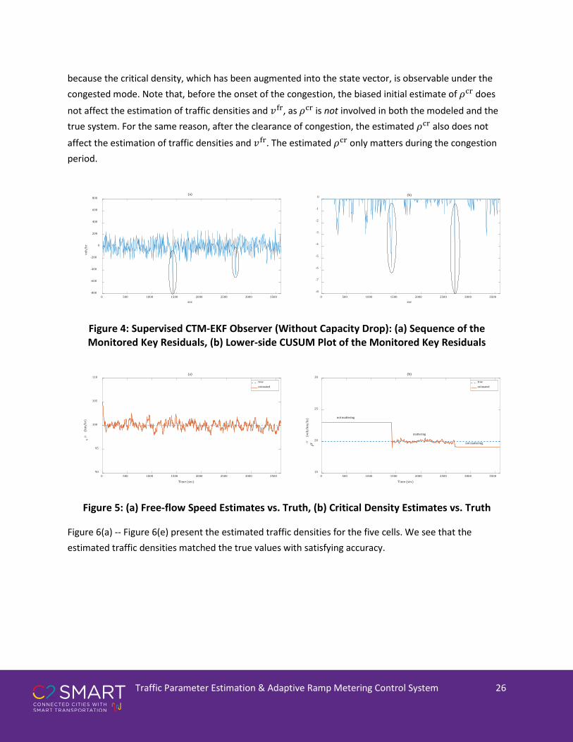
Traffic Parameter Estimation & Adaptive Ramp Metering Control System 26
because the critical density, which has been augmented into the state vector, is observable under the congested mode. Note that, before the onset of the congestion, the biased initial estimate of 𝜌𝜌cr does
not affect the estimation of traffic densities and 𝑣𝑣fr, as 𝜌𝜌cr is not involved in both the modeled and the true system. For the same reason, after the clearance of congestion, the estimated 𝜌𝜌cr also does not
affect the estimation of traffic densities and 𝑣𝑣fr. The estimated 𝜌𝜌cr only matters during the congestion period.
Figure 4: Supervised CTM-EKF Observer (Without Capacity Drop): (a) Sequence of the Monitored Key Residuals, (b) Lower-side CUSUM Plot of the Monitored Key Residuals
Figure 5: (a) Free-flow Speed Estimates vs. Truth, (b) Critical Density Estimates vs. Truth
Figure 6(a) -- Figure 6(e) present the estimated traffic densities for the five cells. We see that the estimated traffic densities matched the true values with satisfying accuracy.
0 500 1000 1500 2000 2500 3000 3500sec
-800
-600
-400
-200
0
200
400
600
800
veh/
hr
(a)
0 500 1000 1500 2000 2500 3000 3500sec
-8
-7
-6
-5
-4
-3
-2
-1
0 (b)
0 500 1000 1500 2000 2500 3000 3500
Time (sec)
90
95
100
105
110
vfr
(km
/hr)
(a)
true
estimated
0 500 1000 1500 2000 2500 3000 3500
Time (sec)
15
20
25
30
cr (
veh/
km/l
n)
(b)
true
estimated
not mattering
not mattering
mattering

Traffic Parameter Estimation & Adaptive Ramp Metering Control System 27
Figure 6: Traffic Density Estimates for Cell 1 (a), Cell 2 (b), Cell 3 (c), Cell 4 (d), and Cell 5 (e)
Subsection 3.5.2 With Capacity Drop
In this subsection we consider the situation where there is capacity drop associated with congestion, and the true capacity drop proportion is 𝜃𝜃 = 0.1. Figure 7 shows that the proposed supervised observer is still able to capture mode switching correctly. Note that, as shown by Figure 7, because of the capacity drop, the length of the duration of the congestion is longer than the situation where there is no capacity drop.
Figure 8(a) and Figure 8(b) show that, as in the situation of no capacity drop, the proposed supervised observer is still able to estimate the values of the free-flow speed and the critical density with satisfying
0 500 1000 1500 2000 2500 3000 3500
Time (sec)
0
10
20
30
40
50
601
(veh
/km
/ln)
(a)
true
estimated
0 500 1000 1500 2000 2500 3000 3500
Time (sec)
0
10
20
30
40
50
60
2 (v
eh/k
m/l
n)
(b)
true
estimated
0 500 1000 1500 2000 2500 3000 3500
Time (sec)
0
10
20
30
40
50
60
3 (v
eh/k
m/l
n)
(c)
true
estimated
0 500 1000 1500 2000 2500 3000 3500
Time (sec)
0
10
20
30
40
50
60
4 (v
eh/k
m/l
n)
(d)
true
estimated
0 500 1000 1500 2000 2500 3000 3500
Time (sec)
0
10
20
30
40
50
60
5 (v
eh/k
m/l
n)
(e)
true
estimated

Traffic Parameter Estimation & Adaptive Ramp Metering Control System 28
accuracy. Figure 8(c) shows that, as soon as congestion is onset, the proposed supervised observer is able to approximately identify the true value of the capacity drop proportion. Apparently, the capacity drop proportion estimates are not as accurate as those of the free-flow speed and the critical density. However, as stated in the end of Section 1.1.2, online estimation of capacity drop proportion a less important issue, because the objective of many traffic control strategies is to prevent congestion, hence capacity drop, from happening.
Figure 7: Supervised CTM-EKF Observer (With Capacity Drop): (a) Sequence of the Monitored Key Residuals, (b) Lower-side CUSUM Plot of the Monitored Key Residuals
Figure 8: (a) Free-flow Speed Estimates vs. Truth, (b) Critical Density Estimates vs. Truth, (c) Capacity Drop Proportion Estimates vs. Truth
0 500 1000 1500 2000 2500 3000 3500sec
-800
-600
-400
-200
0
200
400
600
800
veh/
hr
(a)
0 500 1000 1500 2000 2500 3000 3500sec
-8
-7
-6
-5
-4
-3
-2
-1
0 (b)
0 500 1000 1500 2000 2500 3000 3500
Time (sec)
90
95
100
105
110
vfr
(km
/hr)
(a)
true
estimated
0 500 1000 1500 2000 2500 3000 3500
Time (sec)
15
20
25
30
cr (
veh/
km/l
n)
(b)
true
estimated
not mattering
mattering
not mattering
0 500 1000 1500 2000 2500 3000 3500
Time (second)
0
0.05
0.1
0.15
0.2(c)
true
estimated
not mattering
not mattering
mattering

Traffic Parameter Estimation & Adaptive Ramp Metering Control System 29
Figure 9(a) through (e) show that, with the influence of capacity drop, the proposed supervised observer is still able to estimate the traffic densities of all the cells accurately.
Figure 9: Traffic Density Estimates for Cell 1 (a), Cell 2 (b), Cell 3 (c), Cell 4 (d), and Cell 5 (e)
Subsection 3.6 Summary
This section proposes to use a supervisor to monitor in real time the EKF residuals of the traffic flow measurement variable at a key freeway location, so that mismatches between the current working mode of the CTM-EKF observer and the traffic mode in reality, if occur, can be captured, from which the supervisor determines for the CTM-EKF observer the instants to switch working modes. It is also tried,
0 500 1000 1500 2000 2500 3000 3500
Time (sec)
0
10
20
30
40
50
60
1 (v
eh/k
m/l
n)
(a)
true
estimated
0 500 1000 1500 2000 2500 3000 3500
Time (sec)
0
10
20
30
40
50
60
2 (v
eh/k
m/l
n)
(b)
true
estimated
0 500 1000 1500 2000 2500 3000 3500
Time (sec)
0
10
20
30
40
50
60
3 (v
eh/k
m/l
n)
(c)
true
estimated
0 500 1000 1500 2000 2500 3000 3500
Time (sec)
0
10
20
30
40
50
60
4 (v
eh/k
m/l
n)
(d)
true
estimated
0 500 1000 1500 2000 2500 3000 3500
Time (sec)
0
10
20
30
40
50
60
5 (v
eh/k
m/l
n)
(e)
true
estimated

Traffic Parameter Estimation & Adaptive Ramp Metering Control System 30
for the first time in relevant literature, to augment capacity drop proportion into the state vector, so that its value can be updated in real time when the bottleneck is active. Simulations show that the proposed supervised CTM-EKF observer is able to correctly detect the instants for mode switching, and thus, is able to generate satisfactory estimates for traffic densities and the traffic flow parameters, including the free-flow speed, the critical density, and the capacity drop proportion.
We emphasize that the primary importance of the proposed supervised CTM-EKF observer is able to completely avoid the issue of mismodeling which is inherent in previous CTM-based traffic state observers. This is because the proposed method does not make decisions on mode switching based on any knowledge of the traffic flow parameters as existing CTM-based observers do, but rather, by judging if the current working mode of the observer is consistent with the true system mode. The judgment is done through examining in real time the residuals of a key system output signal by a supervisor. If at some instant, an anomaly in the residuals is detected, it implies that a mismatch between the observer’s working mode and the true system mode has occurred, so the observer should also switch its working mode. Note that, the fact that abnormal residuals reflect mismatches between the observer’s working mode and the true system mode is independent of the values of the system parameters (in this study, the traffic flow parameters). This is the very goodness of residuals. In other words, no matter what the values of the traffic flow parameters actually are at the moment, if an abnormal residual is identified, it signals a mismatch between the observer’s working mode and the true condition of the system.
Finally, note that the proposed supervised observer’s capability to correct biased initial estimate of the critical density is particularly desirable for feedback ramp metering control which uses the critical density as the set-value. In Section 4, we will integrate the proposed supervised CTM-EKF observer with a feedback-type ramp metering controller.

Traffic Parameter Estimation & Adaptive Ramp Metering Control System 31
Section 4 A Supervised Observer-Based Ramp Adaptive Metering Control System
In Section 3, we have developed a supervised CTM-EKF observer of traffic state and traffic flow parameters that can switch working modes in accordance with the switching of true traffic conditions. In this section, we integrate the supervised CTM-EKF observer with a Proportional-Integral-(PI-)type local ramp metering controller, so that the latter can utilize not only real-time updated traffic density of the control target location, but also real-time updated critical density which serves as the set-value. We call the resulting system the supervised observer-based ramp metering control system.
In the following subsections, we first introduce the PI-type ramp metering controller, and then describe how to integrate the supervised observer and the PI controller, and finally perform a simulation study to compare the results of the supervised observer-based ramp metering control system (or in short the supervised system) with the results of the ordinary observer-based ramp metering control system (or in short the ordinary system) which does not update the traffic flow parameters in real time and thereby can suffer from the issue of mismodeling.
For a general textbook on ramp metering control theory, refer to (Kachroo, 2003).
Subsection 4.1 Ramp Metering Control Using Estimated Density and Critical Density
Subsection 4.1.1 Cell Transmission Model with Merging Traffic
In this subsection we introduce a scheme for determining inflows for a road cell that has an on-ramp, under the general modeling framework of CTM. The scheme is known as the ramp priority merging scheme. Please refer to (W.-L. Jin, 2010) for detailed development for it. Simply speaking, the ramp priority merging scheme gives traffic demand on ramp higher priority than traffic demand in mainline. That is, under this scheme, the merge cell will first try to accommodate as much ramp demand as possible, and then the mainline demand. While there exist other merging schemes, which are discussed in (W.-L. Jin, 2010, 2012; W. Jin & Zhang, 2003), the ramp priority merging scheme is chosen to reflect the fact that in reality ramp traffic has to merge into the mainline timely, and compared with mainline traffic, ramp traffic are more aggressive. Note that, as shown by (W.-L. Jin, 2010), the ramp priority merging scheme is not only consistent with Newell’s merging scheme (Newell, 1993), but also a special case of Daganzo’s priority-based merging traffic scheme for network CTM (C. F. Daganzo, 1995).
Consider a freeway section with an on-ramp merge as depicted by Figure 10. The freeway section has three cells, indexed by m-1, m, and m+1, respectively. The on-ramp merges into cell m.

Traffic Parameter Estimation & Adaptive Ramp Metering Control System 32
Figure 10: A Freeway Section with an On-ramp
The ramp priority merging scheme is presented mathematically as
𝑞𝑞ramp = min�𝐷𝐷ramp,𝑆𝑆𝑚𝑚� (36)
𝑞𝑞𝑚𝑚−1,𝑚𝑚 = min �𝐷𝐷𝑚𝑚−1, max�0,𝑆𝑆𝑚𝑚 − 𝐷𝐷ramp�� (37)
With the fundamental assumption that the there is no more restrictive bottleneck downstream of the on-ramp merge, we claim that if there is a congestion caused by merging, then it will originate from cell m-1, i.e. the immediate upstream cell of the merge cell. This claim is equivalent to the following proposition.
Proposition. Under the CTM framework and with the ramp priority merging scheme defined by (36) and (37), the merge cell, m, will never get oversaturated. That is, its highest reachable traffic density of the merge cell is the critical density, 𝜌𝜌cr.
To show the above Proposition, we will first show the following Lemma.
Lemma. The ramp priority merging scheme defined by (36) and (37) is compatible with the general framework of CTM in that it ensures that under all circumstances, the total inflow from the ramp and the upstream mainline cell will never exceed the supply of the merge cell. That is, 𝑞𝑞ramp + 𝑞𝑞𝑚𝑚−1,𝑚𝑚 ≤ 𝑆𝑆𝑚𝑚
is always true.
Proof:
1. If 𝐷𝐷ramp < 𝑆𝑆𝑚𝑚, then from (36) and (37) we have
𝑞𝑞ramp + 𝑞𝑞𝑚𝑚−1,𝑚𝑚 = 𝐷𝐷ramp + min�𝐷𝐷𝑚𝑚−1,𝑆𝑆𝑚𝑚 − 𝐷𝐷ramp� (38)
1.a. If 𝐷𝐷𝑚𝑚−1 < 𝑆𝑆𝑚𝑚 − 𝐷𝐷ramp, then (38) implies
𝑞𝑞ramp + 𝑞𝑞𝑚𝑚−1,𝑚𝑚 = 𝐷𝐷ramp + 𝐷𝐷𝑚𝑚−1 < 𝑆𝑆𝑚𝑚 (39)
1.b. If 𝐷𝐷𝑚𝑚−1 ≥ 𝑆𝑆𝑚𝑚 − 𝐷𝐷ramp, then (38) implies

Traffic Parameter Estimation & Adaptive Ramp Metering Control System 33
𝑞𝑞ramp + 𝑞𝑞𝑚𝑚−1,𝑚𝑚 = 𝐷𝐷ramp + 𝑆𝑆𝑚𝑚 − 𝐷𝐷ramp = 𝑆𝑆𝑚𝑚 (40)
2. If 𝐷𝐷ramp ≥ 𝑆𝑆𝑚𝑚, then from (36) and (37) we have
𝑞𝑞ramp + 𝑞𝑞𝑚𝑚−1,𝑚𝑚 = 𝑆𝑆𝑚𝑚 + min{𝐷𝐷𝑚𝑚−1, 0} = 𝑆𝑆𝑚𝑚 (41)
In light of the above, we conclude that 𝑞𝑞ramp + 𝑞𝑞𝑚𝑚−1,𝑚𝑚 ≤ 𝑆𝑆𝑚𝑚 under all circumstances. This ends the
proof.
Now we are ready to prove the Proposition.
Proof:
From the conservation law we have
𝜌𝜌𝑚𝑚(𝑘𝑘 + 1) = 𝜌𝜌𝑚𝑚(𝑘𝑘) + ∆𝑡𝑡/3600∆𝑥𝑥/1000
�𝑞𝑞𝑚𝑚−1,𝑚𝑚(𝑘𝑘)+𝑞𝑞ramp(𝑘𝑘)−𝑞𝑞𝑚𝑚,𝑚𝑚+1(𝑘𝑘)� (42)
Suppose that 𝜌𝜌𝑚𝑚(𝑘𝑘) = 𝜌𝜌cr. It suffices to show that 𝜌𝜌𝑚𝑚(𝑘𝑘 + 1) ≤ 𝜌𝜌cr. To this end, assume instead that 𝜌𝜌𝑚𝑚(𝑘𝑘 + 1) > 𝜌𝜌cr, which implies that
𝑞𝑞𝑚𝑚−1,𝑚𝑚(𝑘𝑘) + 𝑞𝑞ramp(𝑘𝑘)− 𝑞𝑞𝑚𝑚,𝑚𝑚+1(𝑘𝑘) > 0 (43)
i.e.
𝑞𝑞𝑚𝑚−1,𝑚𝑚(𝑘𝑘) + 𝑞𝑞ramp(𝑘𝑘) > 𝑞𝑞𝑚𝑚,𝑚𝑚+1(𝑘𝑘) (44)
Since by assumption 𝜌𝜌𝑚𝑚(𝑘𝑘) = 𝜌𝜌cr and because of the fundamental assumption that there is no more restrictive bottleneck downstream, we have
𝑞𝑞𝑚𝑚,𝑚𝑚+1(𝑘𝑘) = 𝐷𝐷𝑚𝑚 = 𝐶𝐶𝐶𝐶𝐶𝐶𝐶𝐶𝑐𝑐𝐶𝐶𝑡𝑡𝑦𝑦 (45)
Plugging (45) in (44) leads to
𝑞𝑞𝑚𝑚−1,𝑚𝑚(𝑘𝑘) + 𝑞𝑞ramp(𝑘𝑘) > 𝐶𝐶𝐶𝐶𝐶𝐶𝐶𝐶𝑐𝑐𝐶𝐶𝑡𝑡𝑦𝑦 (46)
On the other hand, per the Lemma, we have
𝑞𝑞𝑚𝑚−1,𝑚𝑚(𝑘𝑘) + 𝑞𝑞ramp(𝑘𝑘) ≤ 𝑆𝑆𝑚𝑚 ≤ 𝐶𝐶𝐶𝐶𝐶𝐶𝐶𝐶𝑐𝑐𝐶𝐶𝑡𝑡𝑦𝑦 (47)
It is obvious (46) and (47) contradict each other. This ends the proof.
In the above, we have shown that under the CTM framework with the ramp priority merging scheme, congestion due to on-ramp merging originates from the cell that is immediately upstream of the merge

Traffic Parameter Estimation & Adaptive Ramp Metering Control System 34
cell. Therefore, a feedback type ramp metering controller designed based on CTM should choose that cell as the control target cell to regulate the traffic density of that cell to stay around the critical density to prevent congestion from happening.
Subsection 4.1.2 A Proportional-Integral Local Ramp Metering Controller
We consider the following Proportional-Integral (PI) type ramp metering strategy that is similar to the PI-ALINEA (Y. Wang & Papageorgiou, 2006).
𝑐𝑐(𝑘𝑘) = 𝑐𝑐(𝑘𝑘 − 1) − 𝐾𝐾𝑝𝑝[𝜌𝜌tar(𝑘𝑘)− 𝜌𝜌tar(𝑘𝑘 − 1)] + 𝐾𝐾𝐼𝐼[𝜌𝜌cr − 𝜌𝜌tar(𝑘𝑘)] (48)
In (48), 𝑐𝑐 represents metering rate; 𝜌𝜌tar denotes the traffic density of the control target cell, 𝜌𝜌cr is the critical density, and 𝐾𝐾𝑝𝑝 and 𝐾𝐾𝐼𝐼 are feedback gains.
To see why (48) is a Proportional-Integral control law, let’s start from the definition. A PI-control is defined as (Astrom & Murray, 2008b):
𝑢𝑢(𝑡𝑡) = 𝐾𝐾𝑝𝑝𝑒𝑒(𝑡𝑡) + 𝐾𝐾𝐼𝐼 � 𝑒𝑒(𝜏𝜏)𝑡𝑡
0𝑑𝑑𝜏𝜏 (49)
Following this definition, the PI ramp metering control law should be:
𝑐𝑐(𝑡𝑡) = 𝐾𝐾𝑝𝑝[𝜌𝜌cr − 𝜌𝜌tar(𝑡𝑡)] + 𝐾𝐾𝐼𝐼 � [𝜌𝜌cr − 𝜌𝜌tar(𝜏𝜏)]𝑡𝑡
0𝑑𝑑𝜏𝜏 (50)
The discrete version of (41) is:
𝑐𝑐(𝑘𝑘) = 𝐾𝐾𝑝𝑝[𝜌𝜌cr − 𝜌𝜌tar(𝑘𝑘)] + 𝐾𝐾𝐼𝐼 � [𝜌𝜌cr − 𝜌𝜌tar(𝑚𝑚)]𝑘𝑘
𝑚𝑚=0= 𝐾𝐾𝑝𝑝[𝜌𝜌cr − 𝜌𝜌tar(𝑘𝑘 − 1)] −𝐾𝐾𝑝𝑝[𝜌𝜌tar(𝑘𝑘) − 𝜌𝜌tar(𝑘𝑘 − 1)]
+ 𝐾𝐾𝐼𝐼 � [𝜌𝜌cr − 𝜌𝜌tar(𝑚𝑚)] + 𝐾𝐾𝐼𝐼
𝑘𝑘−1
𝑚𝑚=0
[𝜌𝜌cr − 𝜌𝜌tar(𝑘𝑘)]
= 𝑐𝑐(𝑘𝑘 − 1) − 𝐾𝐾𝑝𝑝[𝜌𝜌tar(𝑘𝑘)− 𝜌𝜌tar(𝑘𝑘 − 1)] + 𝐾𝐾𝐼𝐼[𝜌𝜌cr − 𝜌𝜌tar(𝑘𝑘)]
(51)
We see that the right hand side of the last equation of (51) is exactly the same as the RHS of (48). A similar derivation was given in (Y. Wang et al., 2014).
The metering rate computed based on the PI control law will be constrained to ensure that it is feasible. The final adopted metering rate, 𝑐𝑐adopted, is given by (52).

Traffic Parameter Estimation & Adaptive Ramp Metering Control System 35
𝑐𝑐adopted(𝑘𝑘) = max�𝑐𝑐min, min �𝑐𝑐max, min �𝑐𝑐(𝑘𝑘),𝐴𝐴ramp(𝑘𝑘 − 1) +𝑙𝑙ramp_queue(𝑘𝑘)∆𝑡𝑡/3600
��� (52)
In (52), 𝑐𝑐min and 𝑐𝑐max represent the lower and upper bounds of the metering rate, respectively. 𝐴𝐴ramp(𝑘𝑘 − 1) is the arrival flow rate on the ramp over time interval k-1, and serves a proxy to the arrival
flow rate on the ramp for time interval k; 𝑙𝑙ramp_queue(𝑘𝑘) is the queue length on the ramp over time
interval k. The reason that we can only use a “proxy” arrival flow rate on the ramp for time interval k is because in reality, 𝑐𝑐adopted(𝑡𝑡) needs to be computed at the beginning of time interval k so that it can be
imposed over the time interval; however, at that instant, 𝐴𝐴ramp(𝑘𝑘) is not yet known, which can only be
available at the end time interval k. But note that 𝑙𝑙ramp_queue(𝑘𝑘) can be readily known at the beginning
of time interval k, because it can be estimated based on 𝑙𝑙ramp_queue(𝑘𝑘 − 1), 𝑐𝑐adopted(𝑡𝑡 − 1), and
𝐴𝐴ramp(𝑘𝑘 − 1). There are studies dedicated to estimation of 𝑙𝑙ramp_queue from noisy measurements of
𝐴𝐴ramp, e.g. (Lee, Jiang, & Chung, 2013). In this study, for simplicity, we assume that 𝐴𝐴ramp is accurately
known so that 𝑙𝑙ramp_queue can be easily estimated for each step.
The advantage of involving 𝐴𝐴ramp(𝑘𝑘 − 1) + 𝑙𝑙ramp_queue(𝑘𝑘)∆𝑡𝑡/3600
in computing 𝑐𝑐adopted is to prevent the ramp
metering controller from generating a much higher metering rate than the most that can be provided by the ramp, so that an unnecessarily long green phase can be avoided.
Finally, note that, 𝑐𝑐adopted(𝑘𝑘) is generated in a way that only uses a “proxy” arrival flow rate on the
ramp for time interval k, and how much ramp traffic will eventually flow into the mainline over time interval k will depend on the actual arrival flow rate on the ramp over the time interval k, i.e. 𝐴𝐴ramp(𝑘𝑘).
Specifically,
𝐷𝐷ramp(𝑘𝑘) = min�𝑐𝑐adopted(𝑘𝑘),𝐴𝐴ramp(𝑘𝑘) +𝑙𝑙ramp_queue(𝑘𝑘)∆𝑡𝑡/3600 � (53)
The 𝐷𝐷ramp(𝑘𝑘) computed by (53) will then be taken by the ramp priority merging scheme (36) and (37) to
determine how much ramp traffic will flow into the merge cell, i.e. 𝑞𝑞ramp, and how much upstream
mainline traffic will flow into the merge cell, i.e. 𝑞𝑞𝑚𝑚−1,𝑚𝑚.
Subsection 4.1.3 Integrating the supervised CTM-EKF observer with the PI controller
We would like to integrate the supervised CTM-EKF observer developed in Section 3 with the PI-type ramp metering controller introduced above, so that the latter can use both the estimated traffic density of the control target cell and the estimated critical density to compute metering rates. That is,
𝑐𝑐(𝑘𝑘) = 𝑐𝑐(𝑘𝑘 − 1) − 𝐾𝐾𝑝𝑝[𝜌𝜌�tar(𝑘𝑘)− 𝜌𝜌�tar(𝑘𝑘 − 1)] + 𝐾𝐾𝐼𝐼[𝜌𝜌�cr(𝑘𝑘) − 𝜌𝜌�tar(𝑘𝑘)] (54)

Traffic Parameter Estimation & Adaptive Ramp Metering Control System 36
In (54), 𝜌𝜌�tar(𝑘𝑘) and 𝜌𝜌�cr(𝑘𝑘) represent the estimated traffic density of the control target cell and the estimated critical density, respectively.
The integrated system is known as an observer-based control system (Astrom & Murray, 2008a). The conceptual framework of the observer-based ramp metering control system of this study is presented by Figure 11. Note that, the scheme of Figure 11 just represents the general situation where a wide coverage of traffic sensors is available which is common in real world (Choe, Skabardonis, & Varaiya, 2002). However, the proposed supervised observer-based ramp metering control system does not demand a sensing condition as shown in Figure 11 to work effectively. Its design dose not rely on an extensive sensor coverage, so it can also work in situations where only the nearby neighborhood of the on-ramp merge is covered by traffic sensors. This has been verified by simulation.
Figure 11: Conceptual Framework of the Observer-based Ramp Metering Control System
Subsection 4.2 Simulations
In this subsection we examine the performance of the supervised observer-based ramp metering control system by simulations. Specifically, we will compare the control results of the supervised system against the control results of an ordinary observer-based ramp metering control system which can only update the traffic density of the control target location in real time, but not the traffic flow parameters.
The Supervised CTM-EKF Observer
The PI-typeController
ControlTargetCell
RampMergeCell

Traffic Parameter Estimation & Adaptive Ramp Metering Control System 37
Subsection 4.2.1 Simulation setup
The considered freeway section is depicted by Figure 12. There are 10 cells, and each cell is 600 m long. A metered on-ramp merges into cell 9. Hence, cell 8 should be chosen as the control target cell. The mainline has two lanes, and the on-ramp has one lane. The length of the simulation period is 200 min. The time step length is 20 sec. The true 𝜌𝜌cr is set as the following: from 0 to 100 min, it is equal to 22
veh/km/lane; from 100 min to 200 min, it is equal to 19 veh/km/lane. The true 𝑣𝑣fr remains fixed, being 120 km/hr. The jam density is 100 veh/km/lane. The CFL condition is satisfied. The mainline arrival flow rates and ramp arrival flow rates are specified as Figure 13. There are two demand peaks so that two periods of congestion will be created. To ensure the problem to be meaningful, it is assumed that the shock generated at a downstream bottleneck will not reach this on-ramp merge section (Daganzo & Carlos, 1997).
For the supervised system, we intentionally provide it with biased initial estimates for 𝑣𝑣fr and 𝜌𝜌cr, which are 108 km/hr and 25 veh/km/lane, respectively. For the ordinary system, we provide it with perfect initial estimates of these parameters, i.e. 100 km/hr and 22 veh/km/lane, respectively.
Figure 12: Geometry of the Simulated Freeway Section
Figure 13: Mainline and Ramp Arrival Flow Rates for the Simulation Experiment
0 m 6000 m
Cell 1 Cell 8 Cell 9 Cell 10
0 20 40 60 80 100 120 140 160 180 200
min
0
500
1000
1500
2000
2500
3000
3500
4000
veh/
hr
mainline
ramp

Traffic Parameter Estimation & Adaptive Ramp Metering Control System 38
Subsection 4.2.2 Results
a) Results of the supervised observer-based ramp metering control system
In this experiment there are 4 mode switching instants because 2 congested periods are formed. Since cell 8 is the control target cell, it is the residuals of the interface flow rates between cell 8 and cell 9 that should be monitored by the supervisor. Figure 14(a) and Figure 14(b) present the sequence of the monitored residual signals and its lower-side CUSUM plot, respectively. We see from Figure 14(a) that, as expected, at each of the 4 instants when the true system switches between free-flow and congested, the residual signal demonstrates an abnormal decrease from the stationary mean, 0. Although these abnormal decreases are distinguishable to human eyes, they may be difficult to be detected automatically since they are embedded in the very noisy stationary parts of the signals. Figure 14(b) shows that, the lower-side CUSUM is able to make these abnormal decreases to stand out of those stationary white noises so that they can be easily detected automatically.
Figure 14: Supervised Observer-based Ramp Metering Control System: (a) Sequence of the Monitored Key Residuals, (b) Lower-side CUSUM Plot of the Monitored Key Residuals
The estimated 𝑣𝑣fr and 𝜌𝜌cr are compared with their true signals, respectively, as shown by Figure 15(a) and Figure 15(b), respectively. Figure 15(a) shows that the supervised system is able to quickly correct
the biased initial estimate of 𝑣𝑣fr. From Figure 15(b), we see that as soon as the first congested period starts, the supervised system is able to correct the biased estimate of 𝜌𝜌cr; as soon as the second congested period starts, the supervised system is able to adapt to the abrupt change in true 𝜌𝜌cr. Here we remind of the fact that during the three free-flow periods (i.e. those marked by “not mattering" in Figure 15(b)), estimates of 𝜌𝜌cr are not used anywhere within the supervised system, and thus biased estimates of 𝜌𝜌cr during these periods do not affect the results of traffic estimation and control.
0 20 40 60 80 100 120 140 160 180 200
min
-600
-400
-200
0
200
400
600
veh/
hr
(a)
0 20 40 60 80 100 120 140 160 180 200
min
-10
-8
-6
-4
-2
0(b)

Traffic Parameter Estimation & Adaptive Ramp Metering Control System 39
Figure 15: Supervised Observer-based Ramp Metering Control System: (a) Free-flow Speed Estimates vs. Truth, (b) Critical Density Estimates vs. Truth
Figure 16 presents the control results of the supervised system. Referring to Figure 16(a), the blue dotted line is the true 𝜌𝜌cr; the red solid line is the true traffic density of the control target cell, 𝜌𝜌tar as a result of the ramp metering control. We see that, during both congested periods, the supervised system is able to effectively accomplish the control objective -- to keep 𝜌𝜌tar close to the true 𝜌𝜌cr, despite the
facts that it is provided with biased initial knowledge of 𝜌𝜌cr and 𝑣𝑣fr, and that the true 𝜌𝜌cr is time-varying. In particular, it should be noted that the true 𝜌𝜌cr having an abrupt change during the free-flow period between the two congested periods has the same effect of providing a wrong initial estimate of 𝜌𝜌cr to the supervised system at some time when 𝜌𝜌cr is unobservable. However, despite this unfavorable situation, the supervised system is able to update the estimated 𝜌𝜌cr to take into account this change as soon as the second congested period becomes active, and thus manages to keep 𝜌𝜌tar close to the changed true 𝜌𝜌cr. Therefore, the supervised system is able to prevent congestion from happening over the entire simulation period for the entire freeway section, as indicated by Figure 16(b).
Figure 16: Control Result of the Supervised System: (a) Traffic Densities of the Control Target Cell, (b) Traffic Density Contour of the Entire Freeway Section
0 20 40 60 80 100 120 140 160 180 200
Time (min)
90
95
100
105
110v
fr (
km/h
r)(a)
true
estimated
0 20 40 60 80 100 120 140 160 180 200
Time (min)
10
15
20
25
30
cr (
veh/
km/l
n)
(b)
true
estimated
not mattering
not mattering
not mattering
mattering
mattering
0 20 40 60 80 100 120 140 160 180 200
min
0
10
20
30
40
50
veh/
km/l
n
(a)
cr
tar
(b)
0 20 40 60 80 100 120 140 160 180 200
min
1000
2000
3000
4000
5000
m
0
5
10
15
20
25
30
35
40
45
50

Traffic Parameter Estimation & Adaptive Ramp Metering Control System 40
b) Results of the ordinary observer-based ramp metering control system
On the other hand, refer to Figure 17 which presents control results of the ordinary system. The blue dotted line is still the true 𝜌𝜌cr; the red solid line is the true traffic density of the control target cell, 𝜌𝜌tar as a result of the ramp metering control. As shown by Figure 17(a), with perfect initial knowledge of the traffic flow parameters, the ordinary system successfully keeps 𝜌𝜌tar close to the true 𝜌𝜌cr during the first congested period; however, it fails to keep 𝜌𝜌tar close to the true 𝜌𝜌cr during the second congested period. This is because the ordinary system is unable to adapt to the change in the true 𝜌𝜌cr occurred between the two congested periods, and therefore, after that change, it computes the ramp metering rates based on an outdated 𝜌𝜌cr as well as the consequent wrong estimates of 𝜌𝜌tar. This typical consequence of mismodeling soon ruins the control target cell, and the congestion propagates into the upstream, as shown by Figure 17(b).
Figure 17: Control Result of the Ordinary System: (a) Traffic Densities of the Control Target Cell, (b) Traffic Density Contour of the Entire Freeway Section
c) Results of the control system without an observer
Finally, we also present the result from the control system without an observer at all, as shown by Figure 18. That is, the ramp metering controller computes metering rates based on traffic densities of the control target location that are directly calculated from the noisy interface flow measurements, and the pre-known, fixed-valued critical density. As for the ordinary observer-based control system, we provide perfect initial knowledge of the traffic flow parameters to the control system without an observer. Figure 18(a) shows that, due to the noisy measurements, even with perfect initial knowledge of the critical density, the control system without an observer is unable to keep the traffic density of the control target cell close to the critical density without significant fluctuations; after the true critical density changes the value, the control system without an observer loses track of the true critical density and thus ends up with keeping the traffic density of the control target cell around a wrong set value (i.e. the outdated critical density) with considerable fluctuations.
0 20 40 60 80 100 120 140 160 180 200
min
0
10
20
30
40
50
veh/
km/l
n
(a)
cr
tar
(b)
0 20 40 60 80 100 120 140 160 180 200
min
1000
2000
3000
4000
5000m
0
5
10
15
20
25
30
35
40
45
50

Traffic Parameter Estimation & Adaptive Ramp Metering Control System 41
Figure 18: Control Result of the System Without an Observer: (a) Traffic Densities of the Control Target Cell, (b) Traffic Density Contour of the Entire Freeway Section
Subsection 4.3 Summary
In this section, we integrated the supervised switching-mode EKF observer of traffic state and parameters developed in the previous section with a feedback-type ramp metering controller to form a supervised observer-based ramp metering control system. We employed the ramp priority merging scheme to model interface flows of the merge cell. We showed that, under the framework of the cell transmission model and the ramp priority merging scheme, congestion due to on-ramp merging will always originate from the cell that is immediately upstream of the merge cell, which thus should serve as the control target cell in the feedback ramp metering control system. Through simulation experiments, we demonstrated that, the supervised observer-based ramp metering control system is able to track time variations of the free-flow speed and the critical density, and consequently can maintain the traffic density of the control target cell close to the critical density whose value is not only initially wrongly known but also time-varying. As a result, the supervised-observer based ramp metering system is able to maintain the free-flow traffic condition for the entire freeway section over the whole simulation period.
On the contrary, we showed that an ordinary observer-based ramp metering system, which treats the traffic flow parameters as pre-known and fixed-valued, fails to keep the traffic density of the control target cell close to the critical density after the change of the value of the critical density, and consequently the entire freeway section soon becomes congested.
Moreover, we also showed that, if the traffic density of the control target cell is directly updated using the noisy interface flow measurements and the traffic flow parameters are assumed to be fixed-valued, i.e. no observer at all, then, the ramp metering controller can end up with making the traffic density of the control target cell to significantly fluctuate around a wrong set-value.
0 20 40 60 80 100 120 140 160 180 200
min
0
5
10
15
20
25
30ve
h/km
/ln
(a)
cr
tar
(b)
0 20 40 60 80 100 120 140 160 180 200
min
1000
2000
3000
4000
5000
m
0
5
10
15
20
25
30
35
40
45
50

Traffic Parameter Estimation & Adaptive Ramp Metering Control System 42
Section 5 A Nonlinear Feedback Ramp Metering Policy Adaptive for A Distant Downstream Bottleneck
As discussed in Subsection 2.3, most previous studies in ramp metering control were concerned with managing bottlenecks that are close to the metered on-ramps, in most cases the bottlenecks are caused by the ramp merging traffic themselves. For the much fewer studies that focused on ramp metering for far downstream bottlenecks, most have employed predictors for traffic flow evolution and designed feedback ramp metering control strategies based on the predictors. In these studies, the ramp metering control strategies themselves cannot adapt to the long distances between the metered on-ramps and the downstream bottlenecks. In this Section, we are to develop a feedback ramp metering policy that are directly adaptive to the long distance between the metering on-ramp and a distant downstream bottleneck for which the policy is developed.
We will approach to this problem using reinforcement learning, specifically, Q-learning. In our approach, an intelligent ramp meter agent learns an optimal ramp metering policy such that the capacity of the distant downstream bottleneck can be fully utilized, but not to be exceeded to cause congestion. The learned policy is in pure feedback form in that only the current state of the environment is needed for the agent to determine the optimal metering rate for the current time. No predictions are needed, as anticipations of traffic flow evolutions have been instilled into the nonlinear feedback policy via learning. To deal with the intimidating computational cost associated with the multi-dimensional continuous state-space, the value-function of actions is approximated by an artificial neural network, rather than a conventional lookup table. The mechanism and development of the approximate value-function and how the learning of its parameters is integrated into the Q-learning process is well explained. The learned ramp metering policy demonstrates effectiveness and benign stability, and a satisfactory level of robustness to demand uncertainties.
Subsection 5.1 A Q-Learning Problem with Value-Function Approximation
Subsection 5.1.1 Multi-dimensional continuous state-space
Consider the freeway section depicted by Figure 19. A lane-drop bottleneck exists far downstream of the metered ramp. The ramp meter is supposed to control the flow into the bottleneck through metering the ramp flow so that the bottleneck capacity can be fully utilized but not to be exceeded. To this end, the objective of the ramp metering policy is such that it can maintain the per-lane traffic density of the
control target location to stay close to the desired value, which is 𝜆𝜆2𝜆𝜆1𝜌𝜌cr, where 𝜆𝜆1 and 𝜆𝜆2 denote the
numbers of lanes before and after the lane-drop respectively, and 𝜌𝜌cr is the per-lane critical density, as in previous Sections. Due to the long distance between the bottleneck and the ramp, a standard feedback type ramp metering strategy that only senses and utilizes traffic state near the bottleneck can

Traffic Parameter Estimation & Adaptive Ramp Metering Control System 43
perform poorly due to a lack of anticipation capability. Therefore, a main requirement in designing our reinforcement learning approach is that it needs to take into account traffic densities measured along the long stretch between the ramp and the bottleneck, so that an anticipation capability can be learned. Since the computational cost of Q-learning grows exponentially with the increase of the dimension of state-space, it would not be computationally cost-effective to take into account measurements at too many places. As a result, three representative places are selected. They are located at the two ends and the middle of the stretch, respectively. Such a treatment at one hand enables the intelligent ramp meter agent to learn to anticipate the evolutions of traffic flow along the stretch, at the other hand limits the computational cost associated with the learning. Note that the place of the downstream end of the stretch happens to be the control target location, whose traffic density will be regulated to stay close to the desired value by ramp metering. Therefore, the first three state variables of the proposed Q-learning problem are traffic densities of the three representative places, denoted by 𝜌𝜌1, 𝜌𝜌2 and 𝜌𝜌3 respectively.
The fourth and also the last state variable is known as the estimated traffic demand on the ramp, denoted by 𝐷𝐷�ramp. This state variable is needed because, to learn how much flow from the ramp should
be released into the mainline, the intelligent ramp meter agent needs to know not only the traffic densities of the three representative mainline locations, but also the current (estimated) traffic demand on the ramp to avoid picking up a metering rate that is too high. The meaning of the notations of (55) are exactly the same as defined in Subsection 4.1.2. The reason to use 𝐴𝐴ramp(𝑘𝑘 − 1) rather than
𝐴𝐴ramp(𝑘𝑘) has also been given in Subsection 4.1.2.
𝐷𝐷�ramp(𝑘𝑘) ≐ 𝐴𝐴ramp(𝑘𝑘 − 1) +𝑙𝑙ramp_queue(𝑘𝑘)∆𝑡𝑡/3600
(55)
To summary, the state vector contains four continuous variables, i.e. �𝜌𝜌1 𝜌𝜌2 𝜌𝜌3 𝐷𝐷�ramp�𝑇𝑇
, resulting in a
four-dimensional continuous state-space.
Figure 19: The Four Continuous State Variables: Traffic Densities at Three Select Mainline Locations and Estimated Traffic Demand on Ramp

Traffic Parameter Estimation & Adaptive Ramp Metering Control System 44
Subsection 5.1.2 State-dependent action space
The actions in the proposed approach are composed of discrete ramp metering rates, as in (Schmidt-Dumont & Van Vuuren, 2015), ranging from the lowest allowable metering rate, 𝑐𝑐min, to the highest allowable metering rate, 𝑐𝑐max. The values of 𝑐𝑐min and 𝑐𝑐max and the number of discrete metering rates are up to user's specification, and are flexible in the proposed approach. In Subsection 5.2, an example of such a specification is given, which is consistent with the requirements of the so-called “full traffic cycle” (Papageorgiou & Papamichail, 2008) signal policy for ramp metering so that the results can be implemented by a traffic light. At any time step, the set of admissible actions may not necessarily consist of all the specified discrete metering rates; it is bounded from above by the estimated traffic demand on the ramp defined by (55). Such a treatment will prevent the agent from picking up a metering rate that is higher than the ramp traffic demand, hence may enhance the learning efficiency. Thus, the action-space at any time step is state-dependent. To emphasize this point, the action-space is written as 𝐴𝐴(𝐬𝐬), as will be seen in the remainder of this section.
Subsection 5.1.3 Reward
The rewards earned by the intelligent ramp meter agent during the learning should reflect the objective of the ramp metering policy to be learned. As introduced above, the objective of the ramp metering policy to be learned is to maintain the traffic density of the control target location, 𝜌𝜌3, to stay close to
the desired value, 𝜆𝜆2𝜆𝜆1𝜌𝜌cr. Therefore, the reward function is defined as:
𝑅𝑅 ≐ 𝑘𝑘 � 𝜌𝜌3 −𝜆𝜆2𝜆𝜆1𝜌𝜌cr� (56)
In (56), 𝑅𝑅 is the reward received by the agent for resulting in 𝜌𝜌3; 𝑘𝑘 is a user-defined negative constant value, serving as a scaling factor; the other notations have been defined earlier. The implication of this reward design is straightforward. That is, it penalizes the traffic density of the control target location for deviating from the desired value. Similar reward designs have been applied by (Fares & Gomaa, 2014; Li, Liu, Xu, Duan, & Wang, 2017; Schmidt-Dumont & Van Vuuren, 2015; C. Wang, Zhang, Xu, Li, & Ran, 2019). In our approach, the reward is a function of only the state resulting from taking an action; but in general, depending on needs, the reward can be a function of the states both before and after taking an action, as well as the action itself (Sutton & Barto, 2018).
Subsection 5.1.4 Value-function approximation by an artificial neural network
If a lookup table method were to be used, the four-dimensional continuous state-space needs to be approximated (discretized) first. If, for example, using the simple aggregation method for approximating

Traffic Parameter Estimation & Adaptive Ramp Metering Control System 45
the continuous state-space, the range of the traffic density is aggregated into 40 intervals, and the range of the estimated traffic demand on the ramp is aggregated into 20 intervals, then there will be as many as 403 × 20, i.e. 1.28 million discrete states. If the action-space consists of 20 metering rates, it implies that the dimension of the resulting lookup table is 1.28 million by 20. That means, there will be a total of 25.6 million action values (i.e. Q-values) to learn, which will be computationally extremely demanding. This motivates the introduction of value-function approximation.
We apply an artificial neural network (ANN) to serve as the approximate value-function. The role of this approximate value-function in the Q-learning process is, at each time step, it takes in the values of all the state variables, i.e. 𝜌𝜌1, 𝜌𝜌2, 𝜌𝜌3, and 𝐷𝐷�ramp, based on which it computes the values for all the
available actions. Therefore, the approximate value-function maps the state vector to the action-value vector. In general, a value-function approximated by an ANN is a nonlinear mapping:
𝐴𝐴𝑁𝑁𝑁𝑁:ℝ|𝑆𝑆| → ℝ|𝐴𝐴| (57)
In (57), 𝐴𝐴𝑁𝑁𝑁𝑁 represents the value-function approximated by an ANN; |𝑆𝑆| and |𝐴𝐴| denote the dimensions of the state-space and action-space, respectively.
a) State Encoding
In many cases, the state variables are not directly fed into the ANN; they are first transformed into some other variables called features (Bertsekas, 2019; Sutton & Barto, 2018), which will then be taken by the ANN. Such a transformation is known as state encoding or feature extraction (Bertsekas, 2019; Sutton & Barto, 2018). As pointed out by (Bertsekas, 2019), state encoding can be instrumental in the success of value-function approximation, and with good state encoding, the ANN needs not to be very complicated. The state encoding method used by this study is a simple version of the tile coding method (Sutton & Barto, 2018), described as follows. For each of the four continuous state variables, its value range is divided into equal discrete intervals that do not overlap with each other; as a result, at any time step, the sampled value of a state variable will fall into one of the intervals that collectively cover the value range of this state variable; the interval into which the sampled value of this state variable falls will be given the value 1, while all the others will be given the value 0. Such a state encoding treatment can give the ANN much stronger stimuli than a treatment can give that simply normalizes state variables to have continuous values between 0 and 1. To emphasize the fact that the feature vector is a function of the state vector, in this section the feature vector is written as 𝐱𝐱(𝐬𝐬), as can be seen in the remainder of this section.
b) Structure of the Value-Function Approximated by ANN

Traffic Parameter Estimation & Adaptive Ramp Metering Control System 46
The feature vector, 𝐱𝐱(𝐬𝐬), is then taken by the ANN. The ANN works in the following way. First, through a linear mapping which is specified by a weight matrix, 𝐖𝐖, it generates the so-called raw values (Gosavi, 2015). Subsequently, each of these raw values is transformed by a nonlinear function, e.g. a sigmoid function, to obtain the so-called threshold values (Gosavi, 2015). Such a nonlinear transformation is also known as activation (Goulet, 2020). Then, the threshold values are transformed again through a linear mapping which is specified by another weight matrix, 𝐕𝐕. Finally, the newly transformed values are added by a vector of coefficients, 𝐜𝐜, known as the bias coefficients (Gosavi, 2015), yielding the outputs from the ANN, i.e. the (approximate) action-value vector, 𝐪𝐪�. Therefore, we see that the ANN is characterized by three sets of parameters, i.e. 𝐖𝐖, 𝐕𝐕, and 𝐜𝐜. In other words, the value-function approximated by the ANN is parameterized by 𝐖𝐖, 𝐕𝐕, and 𝐜𝐜. The mapping from the input state vector to the output action-value vector can thus be written in a compact form as:
𝐪𝐪� = 𝐴𝐴𝑁𝑁𝑁𝑁(𝐱𝐱(𝐬𝐬);𝐖𝐖,𝐕𝐕, 𝐜𝐜) (58)
The structure of the ANN described above is presented by Figure 20. The three sets of parameters, 𝐖𝐖, 𝐕𝐕, and 𝐜𝐜, are unknown, and need to be learned through the Q-learning process. The algorithm for solving this Q-learning problem with the value-function approximated by an ANN will be presented in Subsection 5.1.5.
Figure 20: Structure of the Artificial Neural Network that Serves as the Approximate Value-function

Traffic Parameter Estimation & Adaptive Ramp Metering Control System 47
c) Benefit in Computational Cost
It is worth demonstrating the benefit in computational cost brought by introducing the ANN approximate value-function. Recall that we have estimated the computational cost of the conventional lookup table method in the beginning of Section 3.4. To enable a “fair” comparison with the lookup table, for the ANN approximate value-function, we also assume that the value range of each traffic density variable is divided into 40 intervals, and the value range of the estimated traffic demand on the ramp is divided into 20 intervals. This implies that there is a total of 40 × 3 + 20, i.e., 140 state features. Furthermore, assume that the number of hidden nodes is determined to be 3 times of the number of input features, which has been found to be sufficient to yield good learning results in this study. This implies that the dimension of the weight matrix 𝐖𝐖, is 140 × 420. Still assume that there are 20 available metering rates as in the lookup table case. This implies that the dimension of the weight matrix 𝐕𝐕 is 420 × 20 and the dimension of the bias coefficient vector 𝐜𝐜 is 20. As a result, there are a total of 67,220 unknown parameters to learn. Compared with the 25.6 million action values (i.e. Q-values) to learn for the lookup table method, the benefit in computational cost brought by the value-function approximation is tremendous.
Subsection 5.1.5 The learning algorithm
As shown above, thanks to the approximate value-function, the computational cost of learning can be profoundly reduced. The price is that the learning algorithm will no longer be as straightforward as lookup table methods. For a lookup table method, for any encountered state-action pair, the new Q-value computed by the so-called temporal-difference (TD) rule is directly used to replace the original Q-value in the lookup table. In general, the TD rule of Q-learning is defined as (Sutton & Barto, 2018).
𝑄𝑄new(𝐬𝐬,𝐶𝐶) = 𝑄𝑄old(𝐬𝐬,𝐶𝐶) + 𝛼𝛼 �𝑅𝑅(𝐬𝐬,𝐶𝐶, 𝐬𝐬′) + 𝛾𝛾 max𝑏𝑏∈𝐴𝐴(𝐬𝐬′)
𝑄𝑄(𝐬𝐬′,𝑏𝑏) −𝑄𝑄old(𝐬𝐬,𝐶𝐶)� (59)
In (59), 𝐬𝐬 and 𝐬𝐬′ denote states before and after taking the action, respectively; 𝐶𝐶 and 𝑏𝑏 denote actions; 𝐴𝐴 is the state-dependent action-space; 𝑅𝑅 represents the reward received by the agent moving from state 𝐬𝐬 to state 𝐬𝐬′ by taking action 𝐶𝐶; 𝛼𝛼 is the learning rate; 𝛾𝛾 is the discounting factor. In our approach, the reward 𝑅𝑅 depends only on the state after taking the action, as described in Subsection 5.1.3.
For a value-function approximation-based method, however, replacements of Q-values in a lookup table are no longer applicable, as there is not a lookup table at all; instead, at each time step, the original and new Q-values are jointly used to update the parameters of the approximate value-function. In other words, unlike a lookup table method for which a final lookup table filled by converged Q-values will be the ultimate outcome of the learning process, a value-function approximation-based method uses Q-

Traffic Parameter Estimation & Adaptive Ramp Metering Control System 48
values as training data to calibrate the parameters of the approximate value-function, and the Q-values will not be part of the ultimate outcome of the learning process. This is a distinct difference between the two kinds of methods. It is worth noting that the calibration of the parameters of the approximate value-function is itself a learning problem. Specifically, it is an incremental supervised learning problem. Refer to Algorithm 1. It is incremental as information encapsulated in the datum generated at each time step (i.e. the new Q-value) needs to be absorbed by the parameters as soon as it becomes available. It is supervised as the target output (i.e. the new Q-value) for the ANN is specified at each time step. In this study, the method for evaluating the gradient of the approximate Q-value function with respect to the ANN weights is the so-called incremental back-propagation algorithm (Gosavi, 2015).
The above mechanism of updating the ANN weights under the framework of Q-learning is classical and can be found in textbook (Gosavi, 2015). The corresponding pseudocode is presented by Table 3. In Table 3, we use 𝑞𝑞� to represent the approximate Q-value function, i.e., the ANN. There are two minor abuses of notation (but in consistent with most literature) in Table 3 for the convenience of presentation: By argmax
𝑎𝑎∈𝐴𝐴(𝐬𝐬) 𝑞𝑞�(𝐱𝐱(𝐬𝐬);𝐖𝐖,𝐕𝐕, 𝐜𝐜), we mean the metering rate of the highest action-value
among all admissible metering rates under the current state 𝐬𝐬. Similarly, by max𝑎𝑎∈𝐴𝐴(𝐬𝐬)
𝑞𝑞�(𝐱𝐱(𝐬𝐬);𝐖𝐖,𝐕𝐕, 𝐜𝐜) we
mean the highest admissible action-value under the current state 𝐬𝐬.
Input Data: Mainline and on-ramp traffic demands Output: Calibrated weights of the artificial neural network that serves as the approximate value-function Initialization: Specify 𝛼𝛼, 𝛾𝛾; Set 𝐖𝐖,𝐕𝐕, 𝐜𝐜 to small random numbers (Gosavi, 2015) while episode reward not yet converged do
Set the freeway network as empty Initialize the state 𝐬𝐬 while not the end of this episode do
1. Determine ramp metering rate 𝐶𝐶 according to the 𝜀𝜀-greedy policy 2. Simulate using 𝐶𝐶 to obtain the new state 𝐬𝐬′ 3. Compute reward 𝑅𝑅 based on 𝐬𝐬′ 4. Compute 𝑄𝑄old:
𝑄𝑄old ← 𝑞𝑞�(𝐱𝐱(𝐬𝐬), 𝐶𝐶;𝐖𝐖,𝐕𝐕, 𝐜𝐜) 5. Compute 𝑄𝑄next:
𝑄𝑄next ← max𝑏𝑏∈𝐴𝐴(𝐬𝐬′)
𝑞𝑞�(𝐱𝐱′(𝐬𝐬′);𝐖𝐖,𝐕𝐕, 𝐜𝐜)
6. Compute 𝑄𝑄new using the TD updating rule defined by (59): 𝑄𝑄new ← 𝑄𝑄old + 𝛼𝛼(𝑅𝑅 + 𝛾𝛾𝑄𝑄 next − 𝑄𝑄old)
7. Update the ANN weights with 𝑄𝑄old being the input and 𝑄𝑄new being the target: 𝐖𝐖,𝐕𝐕, 𝐜𝐜 ← 𝜇𝜇(𝑄𝑄new − 𝑄𝑄old)𝛁𝛁𝐖𝐖,𝐕𝐕,𝐜𝐜𝑞𝑞�(𝐱𝐱(𝐬𝐬), 𝐶𝐶;𝐖𝐖,𝐕𝐕, 𝐜𝐜)
end end
Table 3: Pseudocode of the Algorithm of Q-learning with Value-Function Approximation

Traffic Parameter Estimation & Adaptive Ramp Metering Control System 49
Note 1
It is worth noting that the Step 4 through Step 7 within the inner while loop of the algorithm presented in Table 3 can actually be represented by one compact updating equation. In the following, we show how this can be achieved. Plugging 𝑄𝑄old and 𝑄𝑄next as defined by Step 4 and Step 5, respectively, into 𝑄𝑄new as defined by Step 6, yields:
𝑄𝑄new ← 𝑞𝑞�(𝐱𝐱(𝐬𝐬), 𝐶𝐶;𝐖𝐖,𝐕𝐕, 𝐜𝐜) + 𝛼𝛼 �𝑅𝑅 + 𝛾𝛾 max𝑏𝑏∈𝐴𝐴(𝐬𝐬′)
𝑞𝑞�(𝐱𝐱′(𝐬𝐬′), 𝑏𝑏;𝐖𝐖,𝐕𝐕, 𝐜𝐜) − 𝑞𝑞�(𝐱𝐱(𝐬𝐬), 𝐶𝐶;𝐖𝐖,𝐕𝐕, 𝐜𝐜)� (60)
Plugging 𝑄𝑄old as defined by Step 4 and (60) into Step 7 yields:
𝐖𝐖,𝐕𝐕, 𝐜𝐜 ← 𝜇𝜇 �𝑞𝑞�(𝐱𝐱(𝐬𝐬), 𝐶𝐶;𝐖𝐖,𝐕𝐕, 𝐜𝐜) + 𝛼𝛼 �𝑅𝑅 + 𝛾𝛾 max𝑏𝑏∈𝐴𝐴(𝐬𝐬′)
𝑞𝑞�(𝐱𝐱′(𝐬𝐬′), 𝑏𝑏;𝐖𝐖,𝐕𝐕, 𝐜𝐜) − 𝑞𝑞�(𝐱𝐱(𝐬𝐬), 𝐶𝐶;𝐖𝐖,𝐕𝐕, 𝐜𝐜)�
− 𝑞𝑞�(𝐱𝐱(𝐬𝐬), 𝐶𝐶;𝐖𝐖,𝐕𝐕, 𝐜𝐜)�𝛁𝛁𝐖𝐖,𝐕𝐕,𝐜𝐜𝑞𝑞�(𝐱𝐱(𝐬𝐬), 𝐶𝐶;𝐖𝐖,𝐕𝐕, 𝐜𝐜)
(61)
That is,
𝐖𝐖,𝐕𝐕, 𝐜𝐜 ←μα�𝑅𝑅 + 𝛾𝛾 max𝑏𝑏∈𝐴𝐴(𝐬𝐬′)
𝑞𝑞�(𝐱𝐱′(𝐬𝐬′), 𝑏𝑏;𝐖𝐖,𝐕𝐕, 𝐜𝐜) − 𝑞𝑞�(𝐱𝐱(𝐬𝐬), 𝐶𝐶;𝐖𝐖,𝐕𝐕, 𝐜𝐜)�𝛁𝛁𝐖𝐖,𝐕𝐕,𝐜𝐜𝑞𝑞�(𝐱𝐱(𝐬𝐬), 𝐶𝐶;𝐖𝐖,𝐕𝐕, 𝐜𝐜) (62)
Denote 𝜂𝜂 ≐ 𝜇𝜇𝛼𝛼, (62) can be re-written as
𝐖𝐖,𝐕𝐕, 𝐜𝐜 ← 𝜂𝜂 �𝑅𝑅 + 𝛾𝛾 max𝑏𝑏∈𝐴𝐴(𝐬𝐬′)
𝑞𝑞�(𝐱𝐱′(𝐬𝐬′), 𝑏𝑏;𝐖𝐖,𝐕𝐕, 𝐜𝐜) − 𝑞𝑞�(𝐱𝐱(𝐬𝐬), 𝐶𝐶;𝐖𝐖,𝐕𝐕, 𝐜𝐜)�𝛁𝛁𝐖𝐖,𝐕𝐕,𝐜𝐜𝑞𝑞�(𝐱𝐱(𝐬𝐬), 𝐶𝐶;𝐖𝐖,𝐕𝐕, 𝐜𝐜) (63)
Therefore, (63) can be used in place of Step 4 through Step 7 in the inner while loop of the algorithm presented by Table 3. The form of (63) is popular in many textbooks, e.g. (Sutton & Barto, 2018). However, we feel that it is beneficial from a pedagogical point of view to first present the algorithm in the form of Table 3, which clearly shows how to integrate the Q-learning framework with supervised learning to achieve the goal of calibrating the parameters of the approximate value-function (i.e., the ANN weights in this study).
Note 2
Note that, the algorithm presented in Table 3 applies to deep learning almost directly. The only difference is that for a deep learning case, in the Step 7 within the inner while loop, the gradient of the approximate Q-value function will have to be evaluated for more weights other than 𝐖𝐖,𝐕𝐕, 𝐜𝐜, because more hidden layers are present in a deep learning case. It should be clear that the concept of Q-learning with value-function approximation itself has nothing to do with the concept of deep learning. That is, it can be either deep learning or not. [A similar note applies to policy-based methods, but is out of the scope of discussion of this report.] Indeed, Q-learning with value-function approximation, when having multiple hidden layers in the ANN that serves as the approximate value-function, becomes a deep learning application case, known as a deep Q-network; all the concepts, mechanism, and the algorithm

Traffic Parameter Estimation & Adaptive Ramp Metering Control System 50
structure presented earlier in this section, remain largely unchanged. Of course, deep learning itself is an extremely profound and exciting area that is fast developing, for which we are not in a position to comment.
It is our opinion that, although deep learning, when combined with reinforcement learning, such as deep Q-networks, can be very powerful optimization tools, however, it is not necessarily true that the more hidden layers, the better. For example, one downside of deep learning is that, given a fixed dimension of the input feature vector, with the increase of the number of hidden layers, the computation time associated with the updating of the ANN weights (i.e. Step 7 within the inner while loop of the algorithm presented by Table 3) grows exponentially. This can be easily observed in practice, and can be easily explained from the derived equations of the back-propagation updating rule of multi-hidden-layer cases. Moreover, as pointed out by (Sutton & Barto, 2018), the efficiency of the back-propagation algorithm may be undermined with the increase of the number of hidden layers in an ANN. Actually, as pointed out by (Bertsekas, 2019), with good state encoding, the ANN needs not to be very complicated.
However, if one wants to avoid sophisticated state-encoding method, but instead directly feeds the multi-dimensional continuous state vector to the ANN, then a deep ANN may be necessary. Moreover, if the engineering problem at hand for which one wants to resolve using approximate reinforcement learning is complicated enough, then an ANN with only one hidden layer may not be sufficient to reveal an optimal solution.
Finally, we note that the setting of the hyperparameters can be very influential to the success and efficiency of reinforcement learning.
Subsection 5.2 Assessments
Subsection 5.2.1 Simulation setting
This section evaluates the performances of the intelligent ramp metering agent trained by the proposed approach. The layout of the experiment freeway section is illustrated by Figure 21. As shown by Figure 21, a lane-drop is located as far as 3500 meters downstream of the metered ramp. Before the lane-drop, there are 3 lanes in the mainline, and after that, there are 2 lanes in the mainline. The ramp has only one lane.
We still employ the CTM as the simulation model. The free-flow speed is set as 120 km/h, the critical density is set as 20 veh/km/ln, and the jam density is set as 100 veh/km/ln. Since the numbers of lanes before and after the lane-drop are 3 and 2 respectively, thus the desired traffic density for the control
target cell is 23
× 20 = 13.33 veh/km/ln.

Traffic Parameter Estimation & Adaptive Ramp Metering Control System 51
Traffic demands of the mainline and ramp are given by Figure 22, similar to many ramp metering studies.
Figure 21: Layout of the Freeway Section used for Assessment
Figure 22: Traffic Demands at the Mainline and the Ramp for Q-learning Experiment
The method described in Section 3.4.1 is applied for state encoding. The value range of each of the three
traffic density variables is equally divided into 40 intervals. That is, �0,𝜌𝜌jam� is equally divided into 40 intervals. The value range of the estimated traffic demand on the ramp is divided into 20 intervals. Unlike the value range of any traffic density variable which has a fixed upper bound, it is not convenient to specify a fixed upper bound for the value range of the estimated traffic demand on the ramp. Admittedly, if a very large upper bound is specified, it can be ensured that any estimated traffic demand on the ramp can fall within the value range. However, this can cause the estimated traffic demand on the ramp to be much lower than the specified upper bound for most of the times, hence may not be efficient. To resolve this issue, it is worth recalling the purpose of state encoding. Recall that, the purpose of state encoding is to facilitate the efficiency of learning through translating the original value of a state variable into some value(s) that is(are) more representable under the specific learning task. Here, the learning task is to determine the ramp metering rate which is bounded by the highest allowable value, 𝑐𝑐max, regardless of the traffic demand on the ramp. Therefore, a reasonable way to discretize the value range of the estimated traffic demand on the ramp is as follows: The range [0, 𝑐𝑐max] is equally divided into 19 intervals; the range (𝑐𝑐max,∞) accounts for the last interval. The above state encoding treatment converts the four-dimensional state vector of continuous variables into a 140-dimensional (40 × 3 + 20 = 140) feature vector of binary variables.
0 1000 2000 3000 4000 5000 6000sec
0
500
1000
1500
2000
2500
3000
3500
4000
4500
veh/
h
mainline demand
ramp demand

Traffic Parameter Estimation & Adaptive Ramp Metering Control System 52
In this experiment, the lowest allowable metering rate, 𝑐𝑐min, is set as 200 veh/hr, and the highest allowable metering rate, 𝑐𝑐max, is set as 1200 veh/h. The range [200, 1200] is equally divided into 10 intervals, resulting in a total of 11 discrete metering rates: {200,400, … ,1200} veh/hr. Such a specification for the action-space is determined following the so-called “full traffic cycle” signal policy for ramp metering (Papageorgiou & Papamichail, 2008), to ensure that the optimal metering rates leaned through the proposed method can be implemented by a traffic light. Note that, {200,400, … ,1200} veh/h is the largest admissible action-space. As introduced in Subsection 5.1.2, in the proposed approach, at any time step, the admissible action-space can be smaller than the largest set, because it is constrained by the estimated traffic demand on the ramp.
The hyperparameters used in the simulation are specified as the following. The number of hidden neurons is set as 3 times of the state features, i.e. 3 × 140 = 420. The determination of this number was based on a considerable number of trial-and-error experiments. If this number is set too big, the training time would be excessively long; if it is set too small, the approximate value-function would not be able to effectively discriminate different state inputs. The discounting factor, 𝛾𝛾, is equal to 0.95. The learning rate of the TD updating rule (59), 𝛼𝛼, is set as such that before the first 0.1 million iterations, it is equal to 0.05, and it is equal to 0.01 afterwards. The learning rate of the back-propagation rule for updating the ANN weights, 𝜇𝜇, is equal to 0.007. The exploration rate, 𝜀𝜀, in the 𝜀𝜀-greedy policy in the Algorithm presented by Table 1, is set as decaying with the increase of the number of iterated episodes (Sutton & Barto, 2018).
Subsection 5.2.2 Results
The left column of Figure 23 compares the resulting traffic density time series of the control target cell among the case of no control, the case of a PI feedback controller, and the case of the proposed approach; the right column of Figure 23 compares the traffic density contours of the entire freeway section among the three cases. It can be seen that, without any control measure, as traffic demands increase, the traffic density of the control target cell soon grows beyond the desired value and hence a congestion initiates from the bottleneck and grows into the upstream. Under the PI feedback ramp metering control, the traffic density of the control target cell can be maintained around the desired value in the large, however, with severe oscillations which propagate into the upstream and influence the whole section. Under the ramp metering policy learned from the proposed approach, the traffic density of the control target cell is maintained to stay close to the desired value with almost no fluctuations, and accordingly, the traffic density contour of the entire freeway section is smoother than the case of the PI controller.

Traffic Parameter Estimation & Adaptive Ramp Metering Control System 53
Figure 23: Comparison of Traffic Densities of the Control Target Cell and the Traffic Density Contours Across the No Control Case (the top row), the PI Feedback Controller Case (the
Middle Row), and the Case of the Proposed Approach (the Bottom Row)
Figure 24 compares the ramp metering rates computed by the PI controller (left) and by the policy learned through the proposed reinforcement learning approach (right). It indicates that the patterns of the two sets of metering rates are quite different. Moreover, microscopically, the metering rates given by the learned policy are very shredded in order to avoid the potential time-delay effects due to the long distance, thanks to the facts that it is a highly nonlinear feedback policy and takes in traffic conditions at multiple locations along the stretch. It is these shredded metering rates that manage to stabilize the traffic density of the control target cell around the desired value with almost no
0 1000 2000 3000 4000 5000 6000
Sec
0
5
10
15
20
25
30
35
40
45
50ve
h/km
/ln
actual value
desired value
0 1000 2000 3000 4000 5000 6000
Sec
500
1000
1500
2000
2500
3000
3500
4000
4500
5000
5500
m
0
5
10
15
20
25
30
35
40
45
50
0 1000 2000 3000 4000 5000 6000
Sec
0
5
10
15
20
25
30
35
40
45
50
veh/
km/l
n
actual value
desired value
0 1000 2000 3000 4000 5000 6000
Sec
500
1000
1500
2000
2500
3000
3500
4000
4500
5000
5500
m
0
5
10
15
20
25
30
35
40
45
50
0 1000 2000 3000 4000 5000 6000
Sec
0
5
10
15
20
25
30
35
40
45
50
veh/
km/l
n
actual value
desired value
0 1000 2000 3000 4000 5000 6000sec
500
1000
1500
2000
2500
3000
3500
4000
4500
5000
5500
m
0
5
10
15
20
25
30
35
40
45
50

Traffic Parameter Estimation & Adaptive Ramp Metering Control System 54
fluctuations, as shown in Figure 23. By contrast, the metering rates given by the PI controller lack subtle variations but can only constantly oscillate with large amplitudes, which results in quite unstable traffic densities of the control target cell, as shown in Figure 23.
Figure 24: Comparison of Camp Metering Rates Computed by the PI Controller (left) and by the Policy Learned Through the Proposed RL Approach (right)
Subsection 5.2.2 Robustness
It is of interest to what extent the learned ramp metering policy can tolerate uncertainties in traffic demands. To this end, the traffic demands are corrupted by different level of white noises. From top to bottom, Figure 25 presents the results for the cases in which the standard deviation of the white noise of the traffic demands is 50, 100, 150, 200 and 250 veh/h, respectively. It can be seen that the metering policy learned from the proposed approach can perform satisfactorily up to the noise level of 200 veh/h; its performance starts to go down as the demand noise grows bigger.
0 1000 2000 3000 4000 5000 6000
Sec
200
400
600
800
1000
1200
veh/
h
0 1000 2000 3000 4000 5000 6000
Sec
200
400
600
800
1000
1200
veh/
h
0 1000 2000 3000 4000 5000 6000sec
0
500
1000
1500
2000
2500
3000
3500
4000
4500
veh/
h
mainline demand
ramp demand
0 1000 2000 3000 4000 5000 6000
Sec
0
5
10
15
20
25
30
35
40
45
50
veh/
km/l
n
actual value
desired value
0 1000 2000 3000 4000 5000 6000sec
500
1000
1500
2000
2500
3000
3500
4000
4500
5000
5500
m
0
5
10
15
20
25
30
35
40
45
50
0 1000 2000 3000 4000 5000 6000sec
0
500
1000
1500
2000
2500
3000
3500
4000
4500
veh/
h
mainline demand
ramp demand
0 1000 2000 3000 4000 5000 6000
Sec
0
5
10
15
20
25
30
35
40
45
50
veh/
km/l
n
actual value
desired value
0 1000 2000 3000 4000 5000 6000sec
500
1000
1500
2000
2500
3000
3500
4000
4500
5000
5500
m
0
5
10
15
20
25
30
35
40
45
50

Traffic Parameter Estimation & Adaptive Ramp Metering Control System 55
Figure 25: Performances of the Ramp Metering Policy Learned Through the Proposed RL Approach Under Traffic Demands with Different Level of White Noises.
Subsection 5.3 Summary
This section proposes a reinforcement learning approach to learn an optimal ramp metering policy for regulating the traffic at a far downstream bottleneck. The ramp metering policy is learned to be adaptive to the long distance between the metered on-ramp and the downstream bottleneck. An artificial neural network replaces the lookup table in the conventional Q-learning approach to serve as the approximate value-function. The state vector is chosen so that a trade-off between the capability to anticipate traffic flow evolutions and the computational cost is achieved. The action space is state dependent to enhance learning efficiency. The tile coding method is employed to convert the continuous state vector to a binary feature vector to give stronger stimuli to the artificial neural network. The experiment results indicate that, the ramp metering policy learned through the proposed approach is able to yield more stable results than a PI feedback controller. Specifically, under the ramp metering policy learned through the proposed approach, the traffic density of the control target cell is successfully maintained to stay close to the desired value with almost no fluctuations. As a result, traffic flow evolutions over the entire freeway section are also smooth. In comparison, with the PI feedback ramp metering, the traffic density of the control target cell oscillates significantly around the desired
0 1000 2000 3000 4000 5000 6000sec
0
500
1000
1500
2000
2500
3000
3500
4000
4500
5000
veh/
h
mainline demand
ramp demand
0 1000 2000 3000 4000 5000 6000
Sec
0
5
10
15
20
25
30
35
40
45
50
veh/
km/l
n
actual value
desired value
0 1000 2000 3000 4000 5000 6000sec
500
1000
1500
2000
2500
3000
3500
4000
4500
5000
5500
m
0
5
10
15
20
25
30
35
40
45
50
0 1000 2000 3000 4000 5000 6000sec
-1000
0
1000
2000
3000
4000
5000
veh/
h
mainline demand
ramp demand
0 1000 2000 3000 4000 5000 6000
Sec
0
5
10
15
20
25
30
35
40
45
50
veh/
km/l
n
actual value
desired value
0 1000 2000 3000 4000 5000 6000sec
500
1000
1500
2000
2500
3000
3500
4000
4500
5000
5500
m
0
5
10
15
20
25
30
35
40
45
50

Traffic Parameter Estimation & Adaptive Ramp Metering Control System 56
value. Consequently, traffic flow evolutions over the entire freeway section also demonstrate considerable instability. The metering policy learned through the proposed approach has also demonstrated some level of robustness in terms of yielding satisfactory results under uncertain traffic demands.

Traffic Parameter Estimation & Adaptive Ramp Metering Control System 57
Section 6 Conclusions and Future Research
Subsection 6.1 Conclusions
Three major objectives have been achieved through this study. First, a supervisor is developed for detecting mismatches between the working mode of the CTM-EKF observer of traffic state and traffic flow parameters and the actual traffic conditions, so that if a mismatch is detected, the supervisor will inform the CTM-EKF observer to switch working mode. The mechanism of the supervisor is innovative and simple. It monitors in real time the sequence of the EKF residuals of a measurement variable at a key location of the freeway, and if an anomaly is detected, it implies that a mismatch has arisen and hence the CTM-EKF observer should switch the working mode. Such a supervisor is superior in that it requires no knowledge of any traffic flow parameter in any sense, and thus is robust to wrong knowledge of the traffic flow parameters. Simulations for a freeway lane-drop bottleneck section demonstrates that the supervised CTM-EKF observer is not only robust to wrong initial estimates of the traffic flow parameters, but also can correctly capture time variations of the traffic flow parameters, and thus can generate satisfactory estimates of both the traffic state and the traffic flow parameters.
Second, the supervised observer is integrated with a feedback-type ramp metering controller to form a supervised observer-based ramp metering control system. Simulations indicate that, the supervised observer-based ramp metering control system can maintain the traffic density of the control target location to stay around the unknown, time-varying critical density so as to maximize mainline traffic efficiency. In contrast, the simulation study also shows that, an ordinary observer-based ramp metering control system that can only estimate the traffic state in real time but assumes fixed-valued traffic flow parameters fails to prevent congestion from happening, due to its inability to adapt to time variations of the traffic flow parameters.
Third, a reinforcement learning approach is developed for training an intelligent ramp metering agent to learn a nonlinear feedback ramp metering policy that can directly adapt to the long distance between the metered on-ramp and a far downstream targeted bottleneck, without the need for a predictor. The merit of the developed approach is that the learned ramp metering policy is in pure feedback form and does not need a predictor for traffic flow propagation to compensate for the time-delay effects due to the long distance, and thus is very convenient in implementation. The simulation study shows that, the learned nonlinear feedback policy is able to fully utilize the capacity of the distant downstream bottleneck but not to exceed it to cause congestion. In contrast, a conventional linear feedback ramp metering controller causes the traffic density of the remote downstream bottleneck to severely oscillate around the desired set value, due to its inability to adapt to the long distance, and leads to significant oscillations between free-flow and congestion conditions that does not damp out.

Traffic Parameter Estimation & Adaptive Ramp Metering Control System 58
Subsection 6.2 Future Research
With the emergence of new sources of traffic measurements, e.g., onboard GPS data, it can be interesting to examine whether integration of these new data sources can improve the performance of the proposed observer, especially under the circumstances of limited loop detector stations.
Second, the observer-based adaptive ramp metering control in this study is achieved in a sense that the estimation and control tasks are separated. Specifically, the observer takes care of the estimation of the traffic state and the traffic flow parameters, and feeds the estimates to the controller to generate control signals. The most outstanding feature of this approach is that the traffic flow parameters are augmented into the state vector so that their values can be estimated along with the traffic state in real time. It can be interesting to achieve adaptive ramp metering control from an alternative, fundamentally different approach, in which the traffic flow parameters are no longer incorporated into the state vector, but instead, enter the controller through an algebraic equation that maps them to unknown control parameters (Ioannou & Sun, 2012). The controller then tunes the controller parameters by processing inputs and outputs of the controller. A challenging component in this approach to our problem is the determination of the algebraic equation, especially considering that our system is mode-switching.
Third, the reinforcement leaning method employed in this study is value-based, which learns the values of state-action pairs and makes action selection decisions based on the learned values. A fundamentally different, yet as well powerful and exciting alternative approach is policy-based, which learns an optimal policy directly, which does not use action values to make decisions on selecting an action. It will be interesting to apply various policy-based methods to the distant downstream bottleneck ramp metering problem.
Fourth, the developed methodologies in this study are assessed by macroscopic traffic flow simulations. It remains a question how well they can fit into real world applications. Although simulations have been widely used as assessment tools in the literature, it is still desirable to figure out a scientific scheme to examine the potential benefit of the developed methodologies in real world applications. While the development of such a scientific scheme will not be a trivial effort in any way, a plausible next step appears to be integrating the proposed methods into microscopic traffic simulation.

Traffic Parameter Estimation & Adaptive Ramp Metering Control System 59
Appendix A Identification of 𝒉𝒉𝒉𝒉 and 𝒉𝒉𝒉𝒉 Values, Accuracy, and Sensitivity Analysis
Subsection A.1 Identification of ℎ1 and ℎ2
The threshold values ℎ1 and ℎ2 are important parameters of the proposed supervisor. In this appendix, we describe the process to determine ℎ1 and ℎ2, and then perform a sensitivity analysis for ℎ1 and ℎ2 with respect to different levels of measurement noises of the interface flows.
Recall that, ℎ1 should be such a value that if at some instant, the absolute value of the lower-side CUSUM has exceeded ℎ1, then it implies that the true system has turned from free-flow mode to congested mode. Similarly, ℎ2 should be such a value that if at some instant, the absolute value of the lower-side CUSUM has exceeded ℎ2, then it implies that the true system has turned from congested mode to free-flow mode. If any or both of ℎ1 and ℎ2 is set too big, the supervisor may miss some mode switching; on the other hand, if it is set too small, the supervisor may give false notifications of mode switching. Therefore, we should identify proper values of ℎ1 and ℎ2 such that most mode switching can be captured, and few false alarms will be given.
Having been clear about the functions of ℎ1 and ℎ2, it is then straightforward to come up with the following heuristic procedure to determine their values. Assume that the system starts as free-flow and that the measurement noise level is fixed.
1. Set both ℎ1 and ℎ2 to be very large values.
2. Determine ℎ1
a) Run the proposed supervised observation program for a sufficiently large number of repetitions (e.g. 50), each time with a different random seed for the measurement noises.
b) For each repetition, identify the smallest lower-side CUSUM during the period before the true system turns congested; name its absolute value as the repetition-based lower bound of ℎ1.
c) Identify the largest repetition-based lower bound of ℎ1 among all the repetitions; name it as the estimated lower bound of ℎ1.
d) Set the value of ℎ1 to be slightly bigger than the estimated lower bound of ℎ1.
3. Determine ℎ2: Plugging in the value of ℎ1 just identified, conduct a process similar to Step 2, but only that now we are concerned with the period after the true system turns congested and before it turns back to free-flow.

Traffic Parameter Estimation & Adaptive Ramp Metering Control System 60
We make four notes for the above procedure. First, for Step 2(a), if the above procedure is to be applied in real practice rather than a simulation-based study like this work, then the treatment “each time with a different random seed for the measurement noises” just needs to be replaced by the treatment ``each time with a different day’s measurement data''.
Second, for Step 2(b), since the procedure is to be carried offline, thus we can always estimate the instants of true system mode switching by observing the interface flow measurements of the key location, regardless of real practice or a simulation-based study.
Third, referring to Step 2(c), the fact that the estimated lower bounds of ℎ1 and ℎ2 are identified based on a sample of repetitions rather than a single run implies that they have taken into account the repetition-to-repetition random fluctuations of the lower bounds of ℎ1 and ℎ2. The larger the sample is, the less chance the proposed supervisor will issue a false alarm of mode switching.
Fourth, the fact that we set the values of ℎ1 and ℎ2 slightly bigger than their estimated lower bounds, respectively, should have made the chance of the proposed supervisor to miss a mode switching to be quite low.
Subsection A.2 Accuracy of ℎ1 and ℎ2 in Capturing True Mode Switching
It would be desired to know the probability the proposed supervisor can correctly capture mode switching of the true system. To this end, a Monte-Carlo method was employed. Specifically, the simulation of Section 3.3 was run for 100 repetitions, with the standard deviation of the Gaussian noises of the interface flow measurements being 100 veh/hr and each repetition using a distinct random seed. Note that all the random seeds used in these 100 repetitions were different from those that had been used for determining ℎ1 and ℎ2 to ensure that the evaluation was meaningful. It turned out that there were only 3 repetitions for which the proposed supervisor captured mode switching wrongly. The accuracy therefore is approximately 97%.
Subsection A.3 Sensitivities of ℎ1 and ℎ2
Because of the procedure by which ℎ1 and ℎ2 are identified, they are able to handle stochasticities in measurements in the ordinary day-to-day sense; that is, with generally fixed level of measurement noises. But it is interesting to examine how the estimated lower bounds of ℎ1 and ℎ2 will change with different levels of Gaussian noises of measurements.
To this end, we set the standard deviation of the measurement noises of the interface flows to be 50 veh/hr, 100 veh/hr, 150 veh/hr, 200 veh/hr and 250 veh/hr, respectively, and then determined ℎ1 and

Traffic Parameter Estimation & Adaptive Ramp Metering Control System 61
ℎ2 under these noise levels, respectively, for the experiment described in Section 3.3 (assuming no capacity drop). The results are summarized in below table.
Standard Deviation of White Gaussian Noise (veh/hr)
50 100 150 200 250
𝒉𝒉𝒉𝒉� 4.7026 5.1865 5.1932 5.7922 6.0580
𝒉𝒉𝒉𝒉� 6.9871 8.2166 8.2007 8.8111 9.7756
Table A1: Estimated Lower Bounds of 𝒉𝒉𝒉𝒉 and 𝒉𝒉𝒉𝒉 under The Influences of Different Standard Deviations of The White Gaussian Noises of The Key Interface Flow Measurements

Traffic Parameter Estimation & Adaptive Ramp Metering Control System 62
References
Abouaïssa, H., Majid, H., & Jolly, D. J. A. J. o. C. (2017). Nonlinear state estimation and control for freeway on‐ramp metering. 19(1), 233-244.
Astrom, K. J., & Murray, R. M. (2008a). Feedback systems. In An introduction for Scientists and Engineers (pp. 275): Princeton Unvirsity Press.
Astrom, K. J., & Murray, R. M. (2008b). Feedback systems. An Introduction for Scientists and Engineers, Princeton.
Aw, A., & Rascle, M. J. S. j. o. a. m. (2000). Resurrection of" second order" models of traffic flow. 60(3), 916-938.
Barratt, B., Atkinson, R., Anderson, H. R., Beevers, S., Kelly, F., Mudway, I., & Wilkinson, P. J. A. E. (2007). Investigation into the use of the CUSUM technique in identifying changes in mean air pollution levels following introduction of a traffic management scheme. 41(8), 1784-1791.
Bellemans, T., De Schutter, B., Wets, G., & De Moor, B. (2006). Model predictive control for ramp metering combined with extended kalman filter-based traffic state estimation. Paper presented at the 2006 IEEE Intelligent Transportation Systems Conference.
Bertsekas, D. P. (2019). Reinforcement learning and optimal control: Athena Scientific Belmont, MA.
Brandi, A., Ferrara, A., Sacone, S., Siri, S., Vivas, C., & Rubio, F. (2017). Model predictive control with state estimation for freeway systems. Paper presented at the 2017 American Control Conference (ACC).
Chi, R., Hou, Z., Jin, S., Wang, D., & Hao, J. J. I. T. o. I. I. (2013). A data-driven iterative feedback tuning approach of ALINEA for freeway traffic ramp metering with PARAMICS simulations. 9(4), 2310-2317.
Choe, T., Skabardonis, A., & Varaiya, P. (2002). Freeway Performance Measurement System: Operational Analysis Tool. Transportation Research Record: Journal of the Transportation Research Board, 1811, 67-75.
Cremer, M. (1980). Simulation und Regelung des Autobahnverkehrs. Paper presented at the Vorträge der Jahrestagung 1979/Papers of the Annual Meeting 1979.
Daamen, W., & Hoogendoorn, S. P. (2007). Flow-density relations for pedestrian traffic. In Traffic and granular flow’05 (pp. 315-322): Springer.
Daganzo, & Carlos, F. (1997). Fundamentals of Transportation and Traffic Operations || Prelims: Pergamon.
Daganzo, C. (1994). The cell transmission model: A dynamic representation of highway traffic consistent with the hydrodynamic theory. Transportation Research Part B: Methodological, 28(4).

Traffic Parameter Estimation & Adaptive Ramp Metering Control System 63
Daganzo, C. F. (1994). The cell transmission model: A dynamic representation of highway traffic consistent with the hydrodynamic theory. Transportation Research Part B: Methodological, 28(4), 269-287.
Daganzo, C. F. (1995). The cell transmission model, part II: network traffic. Transportation Research Part B: Methodological, 29(2), 79-93.
de Souza, F., & Jin, W. (2017). Integrating a Smith Predictor into Ramp Metering Control of Freeways. Paper presented at the Transportation Research Board 96th Annual Meeting, Washington, D.C., United States.
Fares, A., & Gomaa, W. (2014). Freeway ramp-metering control based on reinforcement learning. Paper presented at the 11th IEEE International Conference on Control & Automation (ICCA).
Frejo, J. R. D., & De Schutter, B. J. I. T. o. I. T. S. (2018). Feed-Forward ALINEA: A ramp metering control algorithm for nearby and distant bottlenecks. 20(7), 2448-2458.
Godunov, S. K. (1959). A difference method for numerical calculation of discontinuous solutions of the equations of hydrodynamics. Matematicheskii Sbornik, 89(3), 271-306.
Golob, T. F., & Recker, W. W. J. J. o. t. e. (2003). Relationships among urban freeway accidents, traffic flow, weather, and lighting conditions. 129(4), 342-353.
Gosavi, A. (2015). Simulation-Based Optimization: Parametric Optimization Techniques and Reinforcement Learning: Springer.
Goulet, J.-A. (2020). Probabilistic machine learning for civil engineers: MIT Press.
Greenshields, B., Bibbins, J., Channing, W., & Miller, H. (1935). A study of traffic capacity. Paper presented at the Highway research board proceedings.
Hanlon, P. D., Maybeck, P. S. J. I. T. o. A., & systems, E. (2000). Characterization of Kalman filter residuals in the presence of mismodeling. 36(1), 114-131.
Hegyi, A., Girimonte, D., Babuska, R., & De Schutter, B. (2006). A comparison of filter configurations for freeway traffic state estimation. Paper presented at the 2006 IEEE Intelligent Transportation Systems Conference.
Hou, Z., Xu, J.-X., & Yan, J. J. T. R. P. C. E. T. (2008). An iterative learning approach for density control of freeway traffic flow via ramp metering. 16(1), 71-97.
Ioannou, P. A., & Sun, J. (2012). Robust adaptive control: Courier Corporation.
Jin, W.-L. (2010). Continuous kinematic wave models of merging traffic flow. Transportation Research Part B: Methodological, 44(8-9), 1084-1103.
Jin, W.-L. (2012). The traffic statics problem in a road network. Transportation Research Part B: Methodological, 46(10), 1360-1373.

Traffic Parameter Estimation & Adaptive Ramp Metering Control System 64
Jin, W., & Zhang, H. M. (2003). On the distribution schemes for determining flows through a merge. Transportation Research Part B: Methodological, 37(6), 521-540.
Kachroo, P. (2003). Feedback Ramp Metering in Intelligent Transportation Systems: Springer US.
Kachroo, P., Krishen, K. J. J. o. I. D., & Science, P. (2000). System dynamics and feedback control design problem formulations for real time ramp metering. 4(1), 37-54.
Kachroo, P., Ozbay, K., & Grove, D. E. (2001). Isolated ramp metering feedback control utilizing mixed sensitivity for desired mainline density and the ramp queues. Paper presented at the ITSC 2001. 2001 IEEE Intelligent Transportation Systems. Proceedings (Cat. No. 01TH8585).
Kan, Y., Wang, Y., Papageorgiou, M., & Papamichail, I. J. T. R. P. C. E. T. (2016). Local ramp metering with distant downstream bottlenecks: A comparative study. 62, 149-170.
Kohan, R. R. (2001). Robust state estimation and control of highway traffic systems. National Library of Canada= Bibliothèque nationale du Canada,
Kotsialos, A., Papageorgiou, M., Diakaki, C., Pavlis, Y., & Middelham, F. J. I. T. o. i. t. s. (2002). Traffic flow modeling of large-scale motorway networks using the macroscopic modeling tool METANET. 3(4), 282-292.
Lee, J. B., Jiang, R., & Chung, E. (2013). Traffic Queue Estimation for Metered Motorway On-ramps using Loop Detector Time Occupancies. Paper presented at the 92nd Annual Meeting of the Transportation Research Board, Washington, D.C.
Li, Z., Liu, P., Xu, C., Duan, H., & Wang, W. J. I. t. o. i. t. s. (2017). Reinforcement learning-based variable speed limit control strategy to reduce traffic congestion at freeway recurrent bottlenecks. 18(11), 3204-3217.
Lowrie, P. (1990). Scats, sydney co-ordinated adaptive traffic system: A traffic responsive method of controlling urban traffic.
Lucas, J., & Crosier, R. J. T. (1982). Fast initial response (FIR) for cumulative sum quality control schemes. 24(3), 199-205.
Majid, H., Abouaíssa, H., Jolly, D., & Morvan, G. (2013). State reconstructor for real-time freeway ramp metering. Paper presented at the 2013 10th IEEE INTERNATIONAL CONFERENCE ON NETWORKING, SENSING AND CONTROL (ICNSC).
Meyer, C., Seborg, D., & Wood, R. J. C. E. S. (1976). A comparison of the Smith predictor and conventional feedback control. 31(9), 775-778.
Mihaylova, L., Boel, R., & Hegyi, A. (2007). Freeway traffic estimation within particle filtering framework. Automatica, 43(2), 290-300.
Montgomery, D. C. (2007). Introduction to statistical quality control: John Wiley & Sons.

Traffic Parameter Estimation & Adaptive Ramp Metering Control System 65
Morărescu, I.-C., & Canudas-de-Wit, C. (2011). Highway traffic model-based density estimation. Paper presented at the American Control Conference (ACC), 2011.
Muñoz, L., Sun, X., Horowitz, R., & Alvarez, L. (2003). Traffic density estimation with the cell transmission model. Paper presented at the American Control Conference, 2003. Proceedings of the 2003.
Nantes, A., Ngoduy, D., Bhaskar, A., Miska, M., & Chung, E. (2016). Real-time traffic state estimation in urban corridors from heterogeneous data. Transportation Research Part C: Emerging Technologies, 66, 99-118.
Nanthawichit, C., Nakatsuji, T., & Suzuki, H. (2003). Application of probe-vehicle data for real-time traffic-state estimation and short-term travel-time prediction on a freeway. Transportation Research Record: Journal of the Transportation Research Board(1855), 49-59.
Newell, G. F. (1993). A simplified theory of kinematic waves in highway traffic, part I: General theory, part II: Queueing at freeway bottlenecks, part III: Multi-destination flows. Transportation Research Part B: Methodological, 27(4), 281–313.
Ozbay, K., Yasar, I., & Kachroo, P. (2006a). Development and Evaluation of On-Line Estimation Methods for Feedback Based Freeway Ramp Metering Strategy. Paper presented at the in 85th TRB Annual Meeting.
Ozbay, K., Yasar, I., & Kachroo, P. (2006b). Improved online estimation methods for a feedback-based freeway ramp metering strategy. Paper presented at the Intelligent Transportation Systems Conference, 2006. ITSC'06. IEEE.
Paesani, G., Kerr, J., Perovich, P., & Khosravi, F. (1997). System wide adaptive ramp metering (SWARM). Paper presented at the ITS America Seventh Annual Meeting and Exposition.
Papageorgiou, M., Blosseville, J.-M., & Hadj-Salem, H. (1989). Macroscopic modelling of traffic flow on the Boulevard Périphérique in Paris. Transportation Research Part B: Methodological, 23(1), 29-47.
Papageorgiou, M., & Papamichail, I. J. T. R. R. (2008). Overview of traffic signal operation policies for ramp metering. 2047(1), 28-36.
Payne, H. J. J. M. M. o. P. S. (1971). Model of freeway traffic and control. 51-61.
Qi, C., Hou, Z., & Li, X. (2008). Freeway feedback ramp metering based on neuron adaptive control algorithm. Paper presented at the 2008 International Conference on Intelligent Computation Technology and Automation (ICICTA).
Schmidt-Dumont, T., & Van Vuuren, J. H. J. I. T. o. I. T. S. (2015). Decentralised reinforcement learning for ramp metering and variable speed limits on highways. 14(8), 1.
Seo, T., & Bayen, A. M. (2017). Traffic state estimation method with efficient data fusion based on the Aw-Rascle-Zhang model. Paper presented at the Intelligent Transportation Systems (ITSC), 2017 IEEE 20th International Conference on.

Traffic Parameter Estimation & Adaptive Ramp Metering Control System 66
Seo, T., Kawasaki, Y., Kusakabe, T., & Asakura, Y. J. T. R. P. B. M. (2019). Fundamental diagram estimation by using trajectories of probe vehicles. 122, 40-56.
Seo, T., Kusakabe, T., & Asakura, Y. (2015a). Traffic state estimation with the advanced probe vehicles using data assimilation. Paper presented at the 2015 IEEE 18th International Conference on Intelligent Transportation Systems.
Seo, T., Kusakabe, T., & Asakura, Y. J. T. R. P. C. E. T. (2015b). Estimation of flow and density using probe vehicles with spacing measurement equipment. 53, 134-150.
Seo, T., Tchrakian, T. T., Zhuk, S., & Bayen, A. M. (2016). Filter comparison for estimation on discretized PDEs modeling traffic: Ensemble Kalman filter and Minimax filter. Paper presented at the Decision and Control (CDC), 2016 IEEE 55th Conference on.
Shlayan, N., Kachroo, P. J. J. o. D. S., Measurement,, & Control. (2013). Feedback ramp metering using godunov method based hybrid model. 135(5).
Simon, D. (2006). Optimal state estimation: Kalman, H infinity, and nonlinear approaches: John Wiley & Sons.
Smaragdis, E., Papageorgiou, M., & Kosmatopoulos, E. J. T. R. P. B. M. (2004). A flow-maximizing adaptive local ramp metering strategy. 38(3), 251-270.
Smaragdis, E., & Papageorgiou, M. J. T. R. R. (2003). Series of new local ramp metering strategies: Emmanouil smaragdis and markos papageorgiou. 1856(1), 74-86.
Stengel, R. F. (1994). Optimal control and estimation: Courier Corporation.
Stylianopoulou, E., Kontorinaki, M., Papageorgiou, M., & Papamichail, I. J. T. L. (2019). A linear-quadratic-integral regulator for local ramp metering in the case of distant downstream bottlenecks. 1-9.
Sun, X., Muñoz, L., & Horowitz, R. (2003). Highway traffic state estimation using improved mixture Kalman filters for effective ramp metering control. Paper presented at the Decision and Control, 2003. Proceedings. 42nd IEEE Conference on.
Sutton, R. S., & Barto, A. G. (2018). Reinforcement learning: An introduction: MIT press.
Tampère, C. M., & Immers, L. (2007). An extended Kalman filter application for traffic state estimation using CTM with implicit mode switching and dynamic parameters. Paper presented at the Intelligent Transportation Systems Conference, 2007. ITSC 2007. IEEE.
Thai, J., Prodhomme, B., & Bayen, A. M. (2013). State estimation for the discretized LWR PDE using explicit polyhedral representations of the Godunov scheme. Paper presented at the American Control Conference (ACC), 2013.
Treiber, M., Kesting, A. J. T. F. D. D., Models, & Simulation, S.-V. B. H. (2013). Traffic flow dynamics.

Traffic Parameter Estimation & Adaptive Ramp Metering Control System 67
Wang, C., Zhang, J., Xu, L., Li, L., & Ran, B. J. I. A. (2019). A new solution for freeway congestion: Cooperative speed limit control using distributed reinforcement learning. 7, 41947-41957.
Wang, Y., Kosmatopoulos, E. B., Papageorgiou, M., & Papamichail, I. J. I. T. o. I. T. S. (2014). Local ramp metering in the presence of a distant downstream bottleneck: Theoretical analysis and simulation study. 15(5), 2024-2039.
Wang, Y., & Papageorgiou, M. (2005). Real-time freeway traffic state estimation based on extended Kalman filter: a general approach. Transportation Research Part B: Methodological, 39(2), 141-167.
Wang, Y., & Papageorgiou, M. (2006). Local ramp metering in the case of distant downstream bottlenecks. Paper presented at the 2006 IEEE Intelligent Transportation Systems Conference.
Weng, J., Liu, L., Rong, J. J. D. d. i. n., & society. (2013). Impacts of snowy weather conditions on expressway traffic flow characteristics. 2013.
Work, D. B., Tossavainen, O.-P., Blandin, S., Bayen, A. M., Iwuchukwu, T., & Tracton, K. (2008). An ensemble Kalman filtering approach to highway traffic estimation using GPS enabled mobile devices. Paper presented at the Decision and Control, 2008. CDC 2008. 47th IEEE Conference on.
Yu, H., Koga, S., Oliveira, T. R., & Krstic, M. J. a. p. a. (2019). Extremum Seeking for Traffic Congestion Control with a Downstream Bottleneck.
Zhang, H. M. J. T. R. P. B. M. (2002). A non-equilibrium traffic model devoid of gas-like behavior. 36(3), 275-290.
Zhao, L., Li, Z., Ke, Z., & Li, M. (2019). Distant downstream bottlenecks in local ramp metering: comparison of fuzzy self-adaptive PID controller and PI-ALINEA. In CICTP 2019 (pp. 2532-2542).
Zhao, L., Li, Z., Ke, Z., & Li, M. J. I. I. T. S. (2020). Fuzzy self-adaptive proportional–integral–derivative control strategy for ramp metering at distance downstream bottlenecks. 14(4), 250-256.
Zhou, Y., Chung, E., Cholette, M. E., & Bhaskar, A. (2018). Real-time joint estimation of traffic states and parameters using cell transmission model and considering capacity drop. Paper presented at the 2018 21st International Conference on Intelligent Transportation Systems (ITSC).


