Adaptive NC Path Generation From Massive Point Data With

1

gatsgagr

fpoo

iADAm2

J

Downloa

Dongdong Zhang

Pinghai Yang

Xiaoping Qian1

e-mail: [email protected]

Department of Mechanical, Materials andAerospace Engineering,

Illinois Institute of Technology,Chicago, IL 60616

Adaptive NC Path GenerationFrom Massive Point Data WithBounded ErrorThis paper presents an approach for generating curvature-adaptive finishing tool pathswith bounded error directly from massive point data in three-axis computer numericalcontrol (CNC) milling. This approach uses the moving least-squares (MLS) surface as theunderlying surface representation. A closed-form formula for normal curvature compu-tation is derived from the implicit form of MLS surfaces. It enables the generation ofcurvature-adaptive tool paths from massive point data that is critical for balancing thetrade-off between machining accuracy and speed. To ensure the path accuracy and ro-bustness for arbitrary surfaces where there might be an abrupt curvature change, a novelguidance field algorithm is introduced. It overcomes potential excessive locality ofcurvature-adaptive paths by examining the neighboring points’ curvature within a self-updating search bound. Our results affirm that the combination of curvature-adaptivepath generation and the guidance field algorithm produces high-quality numerical con-trol (NC) paths from a variety of point cloud data with bounded error.�DOI: 10.1115/1.3010710�

Keywords: NC path generation, point-set surface, moving least-squares surface,curvature

IntroductionRapid development of 3D sensing technology has led to the

rowing use of massive point data in product development, suchs reverse engineering, rapid prototyping, manufacturing, and me-rology. Such wide use of massive point data necessitates the re-earch on direct processing of massive point data into suitableeometric models that can be used in downstream product design,nalysis, and manufacturing. This paper presents an approach forenerating adaptive finishing tool paths with bounded error di-ectly from massive point data in three-axis CNC milling.

Existing approaches to path generation from massive point dataace a dilemma: better quality �curvature-adaptive� paths but withainstaking computer-aided design �CAD� model reconstructionr easy �direct� path generation but without guarantee on accuracyr efficiency. More specifically,

1. Existing approaches to NC path generation typically involvea reverse engineering process, i.e., reconstructing the CADmodels or sculptured surfaces �parametric surfaces, such asBeziers or nonuniform rational B-spline �NURBS� patches�from point data �1–3�, and the traditional CAD model basedNC tool path generation methods could then be used. Such areverse engineering process contains various processingsteps, such as smoothing, segmentation, and surface fitting,and it is laborious and far from automatic. Though somecommercial CAD software, such as CATIA and IMAGEWARE,support the surface reconstruction from point data, high-quality surface reconstruction still requires the interactionsfrom the users with advanced knowledge in surface model-ing. Objects of complex geometry or noisy point cloud still

1Corresponding author.Contributed by the Manufacturing Engineering Division of ASME for publication

n the JOURNAL OF MANUFACTURING SCIENCE AND ENGINEERING. Manuscript receivedpril 28, 2008; final manuscript received August 29, 2008; published onlineecember 4, 2008. Review conducted by Burak Ozdoganlar. Paper presented at theSME 2008 Design Engineering Technical Conferences and Computers and Infor-ation in Engineering Conference �DETC2008�, Brooklyn, NY, July 6–August 3,

008.

ournal of Manufacturing Science and EngineeringCopyright © 20

ded 04 Dec 2008 to 216.47.153.148. Redistribution subject to ASM

pose critical challenges for automatic segmentation in re-verse engineering.

2. Alternative approaches �4–8� that can directly generate toolpaths from massive point data without CAD model recon-struction, due to the absence of an underlying surface model,produce NC tool paths strictly based on the discrete pointsthat result in two problems. �1� Without a continuous sur-face, it is difficult to achieve the adaptive forward steps andpath intervals, leading to poor machining efficiency. �2� It isdifficult to control the machining accuracy when the data arenoisy.

Therefore, in this paper, we present an approach that produceshigh-quality NC tool paths directly from massive point data with-out laborious CAD model reconstruction. More specifically, thisapproach uses the moving least-squares �MLS� surface as an un-derlying representation for the point-set surface. A closed-formformula for normal curvature computation is derived from theimplicit form of MLS surfaces. It enables the generation ofcurvature-adaptive tool paths from massive point data that is criti-cal for balancing the trade-off between machining accuracy andspeed. To ensure the accuracy and robustness of the resultingpaths for arbitrary surfaces where there might be an abrupt curva-ture change, a novel guidance field algorithm is introduced. Itovercomes potential excessive locality of curvature-adaptive pathsby examining the neighboring guidance points’ curvature within aself-updating search bound.

Our point-set surface based approach represents many advan-tages over the existing approaches for generating NC paths frommassive point data. Our approach inherits the MLS’s intrinsicability to handle noisy point data. The availability of an underly-ing surface definition, MLS surfaces, enables our approach to gen-erate curvature-adaptive tool paths with bounded error, leading toefficient and accurate NC machining without the painstaking CADmodel reconstruction.

Our main contributions in this paper are as follows.

• Closed-form formula for computing normal curvatures in
MLS surfaces. Based on the implicit definition of MLS sur-
FEBRUARY 2009, Vol. 131 / 011001-109 by ASME

E license or copyright; see http://www.asme.org/terms/Terms_Use.cfm

add

iddiaitw

2

Maemesfr

idwrlt

nsaah

comc

fip

pbaHpmb

0

Downloa

faces, we develop the closed-form formula for computingnormal curvatures in MLS surfaces.

• Curvature-adaptive path generation from massive pointdata. The analytical equations of the normal curvature inMLS surfaces support the adaptive tool path generation,which greatly improves both machining efficiency and ac-curacy.

• Novel guidance field algorithm with the self-updating searchbound. The introduction of a guidance field allows theshrinkage of forward steps when a larger normal curvatureoccurs in the forward machining region. Meanwhile, theside steps can also be adjusted by this guidance field, so theresulting curvature-adaptive paths are guaranteed to havebounded error even for surfaces with abrupt curvaturechanges.

Our results affirm that the combination of the curvature-daptive path generation and the guidance field algorithm pro-uces high-quality NC tool paths from a variety of point cloudata with bounded error.

The remainder of this paper is organized as follows. Section 2ntroduces the related work in NC path generation from pointata. Section 3 presents an overview of our approach. Section 4erives the closed-form formula for computing normal curvaturesn an MLS surface. Section 5 introduces our novel guidance fieldlgorithm and the self-updating search bound. Implementation andllustrative examples are given in Sec. 6. Section 7 discusses po-ential issues in this approach. Finally, conclusions and futureork are presented in Sec. 8.

Related WorkThe study on NC tool path planning has had a very long history.ost of the research related to the sculptured surface machining

ssumes some exact mathematical representations �9–11�. How-ver, thus far, there is limited work on tool path generation fromeasured point data. The prevalent approach is through reverse

ngineering where a sculpture surface representation is recon-tructed. Approaches aiming to directly generate NC tool pathsrom point data without CAD model reconstruction are brieflyeviewed below.

Direct NC path generation from point data. Lin and Liu �4�ntroduced a tool path generation approach directly from pointata with a Z-map method where a constant Z-level point modelas set up. A linear interpolation method was used to create the

egular grid points linked up by line segments. In this method, aarge memory was needed to store the grids, and how to controlhe machining accuracy was not discussed.

Feng and Teng �5� proposed a method where a cutter location-et �CL-net� was established by identifying the forward steps andide steps, and the cutter location points were the weighted aver-ges of the related CL-net nodes. However, due to the absence ofmathematical representation of a continuous surface, the cusp

eight was approximated.Chui and Lee �6� proposed a method where the spheres of the

utter radius rolled across the irregular nodal points and Booleanperations were utilized to trace the cutter locations. However, theachining accuracy was approximated and the adaptive tool paths

ould not be achieved.Park and Chung �7� developed a 2D algorithm to calculate the

nishing tool paths. However, it could only deal with organizedoint data.

With the algorithmic advancement of triangulating massiveoint data and with the wide usage of STL file �12�, triangle meshased methods have been used to generate tool paths. In Ref. �8�,mesh offset method for tool path generation was proposed.owever, the triangulation process is still a complex task becauserefiltering and postprocessing operations are still needed. Theultitude of operations makes it difficult to maintain an error

ound. Adaptive path generation on triangular mesh would be

11001-2 / Vol. 131, FEBRUARY 2009


difficult since the curvature is not directly available on a polygo-nal object and curvature computing thus involves further approxi-mation.

MLS surface. MLS surfaces have proven to be powerful andconvenient in point based geometric processing and graphics ap-plications �13–20�. Salient features of MLS surfaces include theability of handling noise, up-sampling, down-sampling, and so on.Moreover, based on a more general definition of a projection pro-cess �15,16�, a mathematical proof of the convergence of the pro-jection procedure was presented �18,19�. The resulting MLS sur-face was proven to be isotopic to the original sampled surface.

Guidance field algorithm. Our guidance field approach differsfrom the one in Ref. �21� in two important aspects: we sampledense points on the planar paths instead of projecting the originalinput points onto the MLS surface; and we use a self-updatingsearch bound to maintain both the curvature-adaptivity and ma-chining accuracy.

3 OverviewIn this paper, we use the isoplanar method to generate the fin-

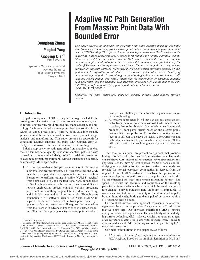
ishing tool paths for three-axis milling with a ball-end tool, al-though other NC path generation strategies can also be used. Spe-cifically, a series of parallel planes, called drive planes, areintersected with the MLS surface defined by the massive pointcloud. The intersection curves are called cutter contact paths �CCpaths�, and the points on the CC paths are called cutter contactpoints �CC points�, shown in Fig. 1. The cutter location paths �CLpaths� are those that connect a series of cutter location points �CLpoints�, which can be converted from CC points. Therefore, theCC point generation is the most important component in our ap-proach.

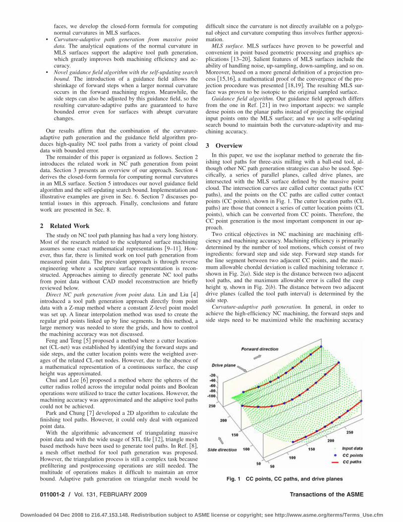
Two critical objectives in NC machining are machining effi-ciency and machining accuracy. Machining efficiency is primarilydetermined by the number of tool motions, which consist of twoingredients: forward step and side step. Forward step stands forthe line segment between two adjacent CC points, and the maxi-mum allowable chordal deviation is called machining tolerance �,shown in Fig. 2�a�. Side step is the distance between two adjacenttool paths, and the maximum allowable error is called the cuspheight �, shown in Fig. 2�b�. The distance between two adjacentdrive planes �called the tool path interval� is determined by theside step.

Curvature-adaptive path generation. In general, in order toachieve the high-efficiency NC machining, the forward steps andside steps need to be maximized while the machining accuracy

Fig. 1 CC points, CC paths, and drive planes

Transactions of the ASME


ns

dcsasd�

ni

ts

Ftca

Fctpva

J

Downloa

eeds to be maintained. Hence the curvature-adaptive forwardteps and side steps are preferred.

Normal curvatures of CC points along two directions, forwardirection �+X direction� and side direction �+Y direction�, are theritical factors in determining forward steps and side steps inculptured surface machining �1,9�. Based on the osculating circlessumption and the machining accuracy requirements, the forwardtep can be determined by the normal curvature along the forwardirection �called the forward normal curvature� �9�, shown as Eqs.1� and �2�.

For the convex case,

�CC = 2R�1 − ��R + r − ��/�R + r��2�1/2 �1�For the concave case,

�CC = 2R�1 − ��R − r − ��/�R − r�2��1/2 �2�

In Eqs. �1� and �2�, R=1 /kforwardN , where kforward

N is the forwardormal curvature, r is the radius of the mill, and � is the machin-ng tolerance.

Similarly, the side step can be determined by the normal curva-ure along the side direction �called the side normal curvature� �1�,hown in Eqs. �3� and �4�.

For the convex case,

(a) (b)

ig. 2 Machining error: „a… tolerance �: R is the normal curva-ure in the forward direction and �cc is the forward step; and „b…usp height �: R� is the normal curvature in the side directionnd �cc is the side step

(a) (b)

ig. 3 Guidance field algorithm overcoming the excessive lo-ality of the curvature effect: „a… abrupt changes of the curva-ure at point A leads to the next CC point at B� resulting in theath bias; and „b… the guidance field algorithm checks the cur-ature in the front region and shrinks the forward step
ccordingly
ournal of Manufacturing Science and Engineering


�cc =R�

�R� + ��R� + r�

��2��R� + r�2 + r2��R� + ��2 − ��R� + r�2 − r2�2 − �R� + ��4

�3�For the concave case,

�cc =R�

�R� − ��R� − r�

��2��R� − r�2 + r2��R� − ��2 − ��R� − r�2 − r2�2 − �R� − ��4

�4�

In Eqs. �3� and �4�, R�=1 /ksideN , where kside

N stands for the sidenormal curvature, r stands for the radius of the ball-end mill, and� stands for the cusp height. The tool path interval depends onboth the side normal curvature and the slope in the side direction�2�. We show in Sec. 4 how we derive normal curvature on MLSsurfaces.

Guidance field for overcoming extreme locality of the curvatureeffect. Although curvature-adaptive NC paths effectively resolvethe trade-off between machining efficiency and accuracy, the lo-cality of curvature may lead to biased paths when the surfacegeometry has an abrupt curvature change. For example, as shownin Fig. 3�a�, the forward normal curvature is small at point A,leading to a long forward step to arrive at point B�. However,between A and B� there exist regions with a much larger normalcurvature, and the machining accuracy thus cannot be maintained.

Therefore, in this paper, we introduce a novel guidance field toproactively identify locations with excessive curvature changethat may bias the paths. The guidance field provides a scalar fielddescription of curvature distribution within the object surface. Aguidance field algorithm would then intelligently search within aself-updating bound for the correct forward step. As shown in Fig.3�b�, the adjusted forward step from the guidance field algorithmis shorter than the initial forward step in the sharp curvaturechange area by querying the guidance field around point A. De-tailed procedures are illustrated in Sec. 5.

4 Closed-Form Formula for Normal Curvature Com-puting in MLS Surfaces

The calculation of the normal curvature from massive pointdata is the key issue in our curvature-adaptive approach. In thispaper, we use an MLS surface as the underlying surface, and thenormal curvature is calculated based on the MLS surface.

4.1 Projection Based MLS Surfaces. The MLS surface wasfirst introduced by Levin �13,14�. Based on Levin’s work, Amentaand Kil �15,16� defined MLS surfaces as the local minimum of anenergy function e�y ,n��x�� along the directions given by a vectorfield n��x�. The MLS surface is defined as

g�x� = n��x�T� �e�y,n��x��y

y=x = 0 �5�

where x and y represent the coordinates of the spatial points, eachdefined as �x ,y ,z�. The normalized n��x� is determined by thenormal vector v�i of the nearby input point qi�Q. If v�i is unavail-able, the covariance matrix can be established to calculate v�i �22�so n��x� can be defined as

n��x� =�qi�Q

v�iG�x,qi�

��qi�Qv�iG�x,qi��

where G�x ,qi�=e−�x − qi�2/h2

is a Gaussian weighting function, inwhich h is the scale factor that determines the width of the Gauss-ian kernel, discussed extensively in Refs. �17,18,23�. The energy

�
function e�y ,n�x�� is defined as
FEBRUARY 2009, Vol. 131 / 011001-3


pp

aso

inf

dp

E

a

Fstts

0

Downloa

e�y,n��x j�� = �qi�Q��y − qi�Tn��x j��2G�y,qi�

Therefore, by tracing the minimum of the local energy, we canroject a spatial point onto the MLS surface. For details of thisrojection process, please refer to Refs. �15,16�.

4.2 Normal Curvature Calculation. In our path generationpproach, two normal curvatures for the forward step and the sidetep are required, as discussed in Sec. 3. In this section, we focusn computing the normal curvature.

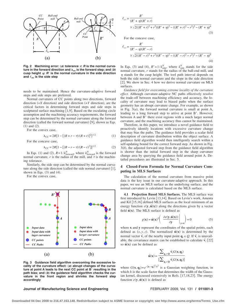
We first compute the curve curvature of CC points along thentersection curve. Based on the surface normal and the curveormal of the CC points, we can then compute the correspondingorward normal curvature, as shown in Fig. 4.

In our work, the drive plane is parallel to the XZ plane and isenoted as y=a, where a is a constant value for a given drivelane. So the CC path on an MLS surface can be represented as

g�x� = n��x,y,z�T��e�y,n��x,y,z��y

�x,y,z�

= 0

y = a� �6�

quation �6� can be simplified as

g�x,z� = n��x,a,z��T��e��y,n��x,a,z��y

�x,a.z�

= 0 �7�

nd

g�x,z� = n��x,a,z��T��e��y,n��x,a,z��y

�x,a.z�

= �qi�Q

2e−�x − qi�2/h2�1 −

1

h2 ��x − qi�Tn��x��2T�

(a) (b)

ig. 4 Surface normal and curve normal. The dense pointstand for the input data. The curve is the CC path and points onhe CC path are the CC points. The dashed arrows representhe surface normal vectors of the CC points, and the solid onestand for the curve normal vectors of the CC points.

· �x − qi� n�x� �8�

h

11001-4 / Vol. 131, FEBRUARY 2009


Hence the curvature on the planar curve, kcurve, can be computed�24�. Based on Eq. �8�, we can denote the normal curvature of thisplanar curve as

kforwardN = kcurve cos � = −

T�g�x,z�� · H�g�x,z�� · T�g�x,z��T

��g�x,z��

· n��x,y,z�� · n��x,a,z�� 9�

where −�T�g�x ,z�� ·H�g�x ,z�� ·T�g�x ,z��T / ��g�x ,z�� representsthe curvature of the implicit planar curve, n��x ,y ,z�� representsthe unit normal vector of the MLS surface shown as the dashedarrows in Fig. 4, and n��x ,a ,z�� represents the unit normal vectorof the implicit curve shown as the solid arrows in Fig. 4, so � isthe angle between n��x ,y ,z�� and n��x ,a ,z��. In Eq. �9�,

�g�x,z� = � �g�x,z��x

�g�x,z��z

is the gradient of g�x ,z�, and the Hessian matrix is

H�g�x,z�� =��2g�x,z��x � x

�2g�x,z��x � z

�2g�x,z��z � x

�2g�x,z��z � z

�and T�g�x ,z�� is the unit tangent vector of the implicit curve

T�g�x,z�� =�−

�g�x,z��z

�g�x,z��x

��−

�g�x,z��z

�g�x,z��x

� =�g�x,z�

��g�x,z��· �0 1

− 1 0�

Therefore, the critical part is to calculate the gradient matrix��g�x ,z�� and the Hessian matrix H�g�x ,z��. From Eq. �8�, we canget

��g�x,z�� = �qi�Q2e−�x − qi�

2/h2� 2

h2 ��x − qi�Tn��x��

· � 1

h2 ��x − qi�Tn��x��2 − 1 · �x − qi�

+ �1 −3

h2 ��x − qi�Tn��x��2 · �n��x� + �T�n��x��

· �x − qi��
The Hessian of g�x ,z� can be represented as
H�g�x,z�� = ��g�x,z�� = �qi�Q−

4

h2e−�x − qi�2/h2� 2

h2 ��x − qi�Tn��x�� · � 1

h2 ��x − qi�Tn��x��2 − 1 · �x − qi�

+ �1 −3

h2 ��x − qi�Tn��x��2 · �n��x� + �T�n��x�� · �x − qi�� · �x − qi�T + 2e−�x − qi�2/h2� 6

h4 ��x − qi�Tn��x��2 −2

h2· �x − qi� · �n�T�x� + �x − qi�T · ��n��x�� +

4

h2e−�x − qi�2/h2

��x − qi�Tn��x�� · � 1

h2 ��x − qi�Tn��x��2 − 1· I −

122 e−�x − qi�

2/h2��x − qi�Tn��x�� · �n��x� + �T�n��x�� · �x − qi�� · �n�T�x� + �x − qi�T · ��n��x��



w

t

S

Npot

5

tmbw

da�

J

Downloa

+ 2e−�x − qi�2/h2�1 −

3

h2 ��x − qi�Tn��x��2 · ��n��x�� + �T�n��x�� + �T��n��x�� · �x − qi��

here I is the identity matrix.Similarly, the intersection curve between the MLS surface and

he plane perpendicular to the drive plane can be expressed as

g�x� = n��x,y,z�T��e�y,n��x,y,z��y

�x,y,z�

= 0

x = b �b is a constant value as to a certain plane��

o the side normal curvature ksideN can be represented as

ksideN = −

T�g�y,z�� · H�g�y,z�� · T�g�y,z��T

��g�y,z��· n��x,y,z�� · n��b,y,z��

�10�

ote that the signs of kforwardN and kside

N have the following explicithysical meanings: if they are negative, the curve is concave;therwise, it is convex. These correspond to different formulas forhe forward step and the side step as described in Sec. 3.

Guidance Field AlgorithmThe purpose of introducing a guidance field in NC path genera-

ion is to maintain the error bound in NC paths, defined as theaximum allowable machining tolerance � and the cusp height �,

y overcoming potential excessive curvature locality for surfacesith abrupt curvature change.The guidance field is a scalar function, which represents the

istribution of the curvature effect over a spatial domain. In ourpproach, on a given drive plane we associate guidance points Pidensely sampled points on the CC paths� with two kinds of guid-

(a)

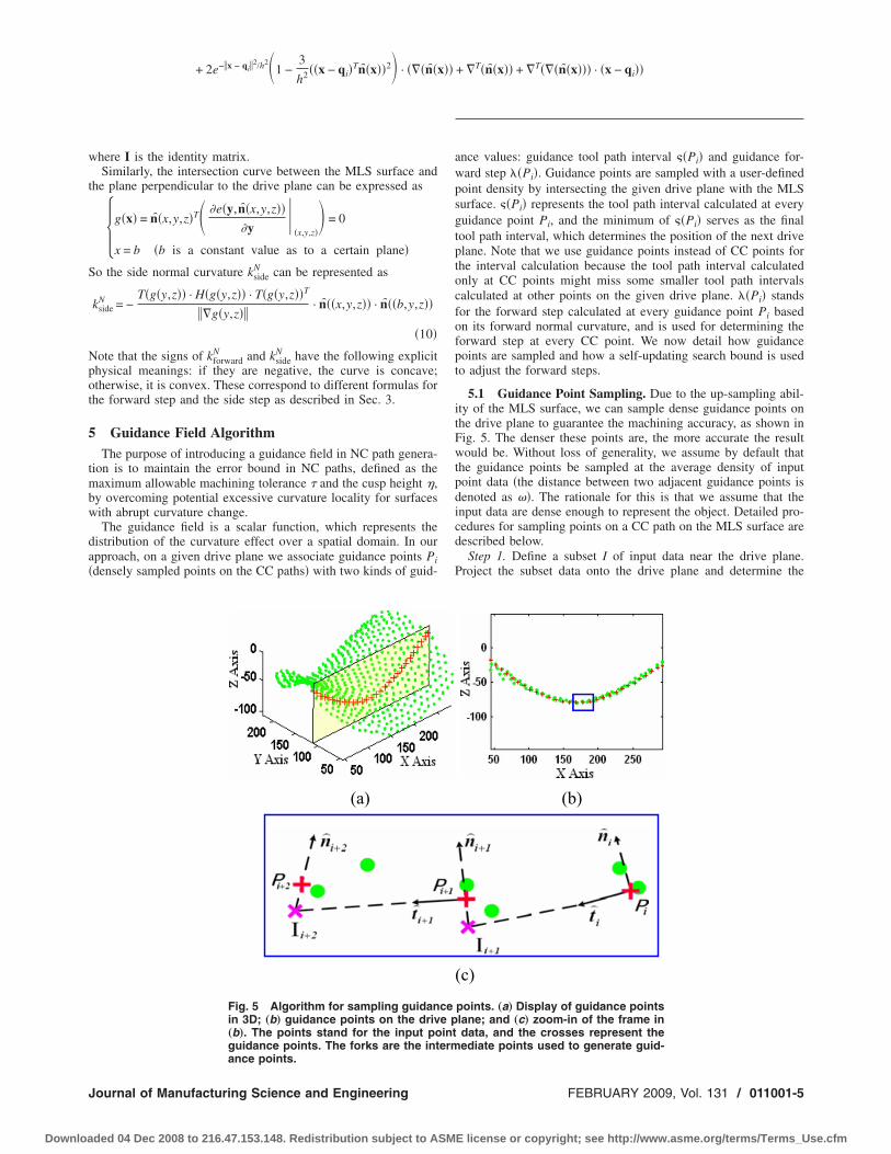
Fig. 5 Algorithm for sampling guidanin 3D; „b… guidance points on the driv„b…. The points stand for the input poguidance points. The forks are the int
ance points.


ance values: guidance tool path interval ��Pi� and guidance for-ward step ��Pi�. Guidance points are sampled with a user-definedpoint density by intersecting the given drive plane with the MLSsurface. ��Pi� represents the tool path interval calculated at everyguidance point Pi, and the minimum of ��Pi� serves as the finaltool path interval, which determines the position of the next driveplane. Note that we use guidance points instead of CC points forthe interval calculation because the tool path interval calculatedonly at CC points might miss some smaller tool path intervalscalculated at other points on the given drive plane. ��Pi� standsfor the forward step calculated at every guidance point Pi basedon its forward normal curvature, and is used for determining theforward step at every CC point. We now detail how guidancepoints are sampled and how a self-updating search bound is usedto adjust the forward steps.

5.1 Guidance Point Sampling. Due to the up-sampling abil-ity of the MLS surface, we can sample dense guidance points onthe drive plane to guarantee the machining accuracy, as shown inFig. 5. The denser these points are, the more accurate the resultwould be. Without loss of generality, we assume by default thatthe guidance points be sampled at the average density of inputpoint data �the distance between two adjacent guidance points isdenoted as ��. The rationale for this is that we assume that theinput data are dense enough to represent the object. Detailed pro-cedures for sampling points on a CC path on the MLS surface aredescribed below.

Step 1. Define a subset I of input data near the drive plane.Project the subset data onto the drive plane and determine the

(b)

(c)

points. „a… Display of guidance pointslane; and „c… zoom-in of the frame indata, and the crosses represent theediate points used to generate guid-

cee pinterm

FEBRUARY 2009, Vol. 131 / 011001-5


seapg

PPd

gptld

wpi

MpIIn�i

w�cts

0

Downloa

tarting trace point IS with the minimum X coordinate and thending trace point IE with the maximum X coordinate. Project ISnd IE to the MLS surface and their corresponding projectedoints are denoted as PS and PE, which are the starting and endinguidance points.

Step 2. Trace all the guidance points Pi �i=1. . .n� from PS to

E. If i�1 and �Pi− PE�, stop the process and outputS , P1 , . . . , Pn , PE as the resulting guidance points on the givenriven plane.

In this algorithm, the most critical issue is to generate the nextuidance point Pi+1 based on the current one Pi. At the currentoint Pi, we first set up a local coordinate system, whose direc-ional axes are defined as the normal vector n�i and its perpendicu-ar direction vector t�i separately, shown in Fig. 5�c�. Then weefine an intermediate point Ii+1 along the direction vector t�i.

Ii+1 = Pi + � · t�i

here � is the sample distance between two adjacent guidanceoints. Finally, we define the next guidance point Pi+1 by project-ng Ii+1 onto the MLS surface.

In Sec. 4.1, the method of projecting a spatial point onto theLS surface was discussed. Here, we introduce the algorithm for

rojecting points onto a planar CC path on the MLS surface. Take

i+1 as an example. We can define the planar normal vector n�i+1 ofi+1, shown in Fig. 5�c�, then we can trace the MLS point along

i+1. Note that any point x on the MLS surface should project totself, which is defined as

��P�x� − x� = 0

here �P�x� represents the corresponding projected point of x13,14�, so the problem is transformed into finding the point thatan project to itself along the direction vector n�i+1. How to findhis point along the line becomes the same issue as the line/MLSurface intersection described in Ref. �25�.

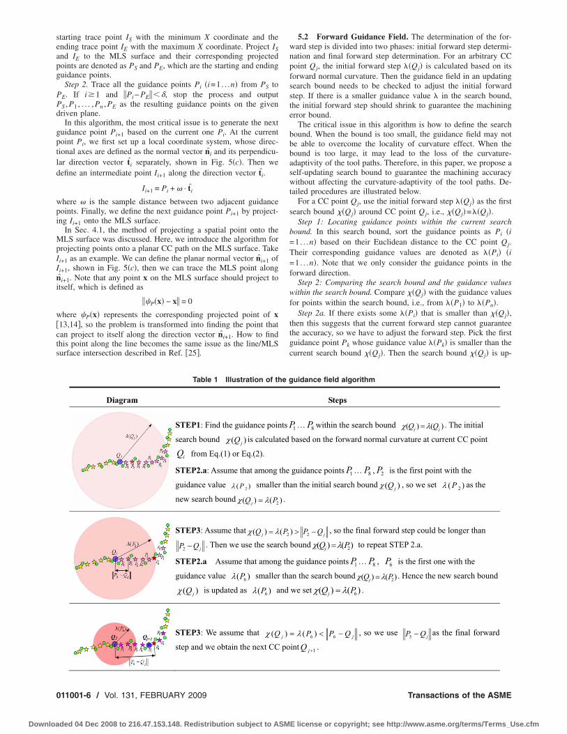
Table 1 Illustration of th

Diagram

STEP1: Find the guidance poin

search bound )( jQχ is calcula

from Eq.(1) or Eq.(2).iQ

STEP2.a: Assume that among

guidance value )( 2Pλ smaller

new search bound ()( 2PQjχ λ=

STEP3: Assume that jQ =)( λχ

jQP −2 . Then we use the sear

STEP2.a Assume that among

guidance value )( 6Pλ smaller

)( jQχ is updated as )( 6Pλ a

STEP3: We assume that Q(χstep and we obtain the next CC

11001-6 / Vol. 131, FEBRUARY 2009


5.2 Forward Guidance Field. The determination of the for-ward step is divided into two phases: initial forward step determi-nation and final forward step determination. For an arbitrary CCpoint Qj, the initial forward step ��Qj� is calculated based on itsforward normal curvature. Then the guidance field in an updatingsearch bound needs to be checked to adjust the initial forwardstep. If there is a smaller guidance value � in the search bound,the initial forward step should shrink to guarantee the machiningerror bound.

The critical issue in this algorithm is how to define the searchbound. When the bound is too small, the guidance field may notbe able to overcome the locality of curvature effect. When thebound is too large, it may lead to the loss of the curvature-adaptivity of the tool paths. Therefore, in this paper, we propose aself-updating search bound to guarantee the machining accuracywithout affecting the curvature-adaptivity of the tool paths. De-tailed procedures are illustrated below.

For a CC point Qj, use the initial forward step ��Qj� as the firstsearch bound ��Qj� around CC point Qj, i.e., ��Qj�=��Qj�.

Step 1: Locating guidance points within the current searchbound. In this search bound, sort the guidance points as Pi �i=1. . .n� based on their Euclidean distance to the CC point Qj.Their corresponding guidance values are denoted as ��Pi� �i=1. . .n�. Note that we only consider the guidance points in theforward direction.

Step 2: Comparing the search bound and the guidance valueswithin the search bound. Compare ��Qj� with the guidance valuesfor points within the search bound, i.e., from ��P1� to ��Pn�.

Step 2a. If there exists some ��Pi� that is smaller than ��Qj�,then this suggests that the current forward step cannot guaranteethe accuracy, so we have to adjust the forward step. Pick the firstguidance point Pk whose guidance value ��Pk� is smaller than thecurrent search bound ��Qj�. Then the search bound ��Qj� is up-

uidance field algorithm

Steps

… within the search bound . The initial1 8P )()( jj QQ λχ =

based on the forward normal curvature at current CC point

guidance points … , is the first point with the1P 8P 2Pn the initial search bound )jQ(χ , so we set )( 2Pλ as the

jQP −> 2) , so the final forward step could be longer than

()( PQjbound )2χ λ= to repeat STEP 2.a.

e guidance points … , is the first one with the1P 8P 6Pn the search bound )( 2P)Qj( λχ = . Hence the new search bound

we set .)()( 6PQj λχ =

jQPP −<= 66 )(λ , so we use jQP −5

1+j

as the final forward

intQ .

e g

tsPted

the

tha

) .

P2(

ch

th

tha

nd

j )po



d

gnsc

v�h

J

Downloa

ated to ��Pk�. Go to Step 3.Step 2b. If there is no ��Pi� smaller than ��Qj�, then this sug-

ests that all the points in the search bound have a smaller forwardormal curvature than that at Qj. Therefore, the initial forwardtep ��Qj� is fine and the final forward step �final=��Qj�. We thusan find the next CC point Qj+1.

Step 3: Comparing the search bound and distances to the pre-iously obtained guidance points. By comparing the distancesPk−1−Qj�, �Pk−Qj�, and by the updating search bound ��Qj�, weave the following three scenarios.

�1� If ��Qj� �Pk−1−Qj�, then the final forward step �final= �Pk−1−Qj� and the next CC point Qj+1 can be found.

�2� If �Pk−1−Qj��Qj� �Pk−Qj�, then the final forward step�final=��Qj�=��Pk� and the next CC point Qj+1 can befound.

�3� If ��Qj�� Pk−Qj�, then the forward step could be longer,so we update the search bound ��Qj�=��Pk� and go to Step2.

(a)

(c)

(e)

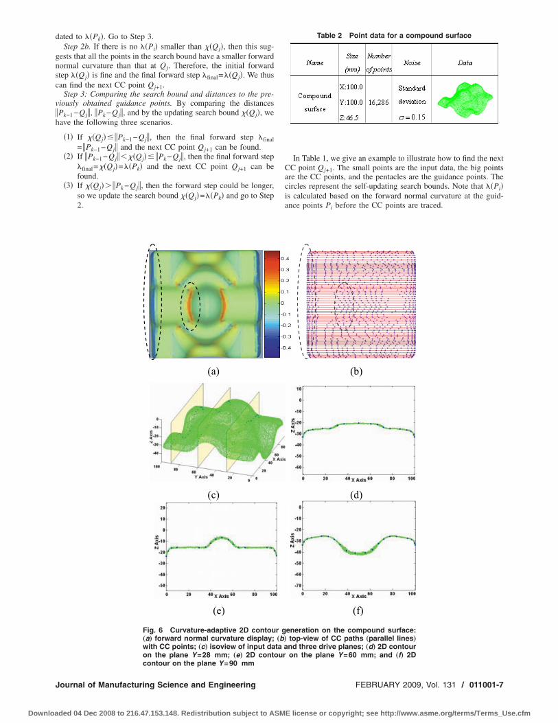
Fig. 6 Curvature-adaptive 2D contou„a… forward normal curvature display;with CC points; „c… isoview of input daon the plane Y=28 mm; „e… 2D cont
contour on the plane Y=90 mm


In Table 1, we give an example to illustrate how to find the nextCC point Qj+1. The small points are the input data, the big pointsare the CC points, and the pentacles are the guidance points. Thecircles represent the self-updating search bounds. Note that ��Pi�is calculated based on the forward normal curvature at the guid-ance points Pi before the CC points are traced.

Table 2 Point data for a compound surface

(b)

(d)

(f)

eneration on the compound surface:top-view of CC paths „parallel lines…nd three drive planes; „d… 2D contouron the plane Y=60 mm; and „f… 2D

r g„b…ta aour

FEBRUARY 2009, Vol. 131 / 011001-7


gganl

0

Downloa

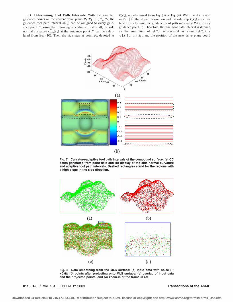
5.3 Determining Tool Path Intervals. With the sampleduidance points on the current drive plane PS , P1 , . . . , Pn , PE, theuidance tool path interval ��Pi� can be assigned to every guid-nce point Pi, using the following procedures. First of all, the sideormal curvature kside

N �Pi� at the guidance point Pi can be calcu-ated from Eq. �10�. Then the side step at point Pi, denoted as

(

Fig. 7 Curvature-adaptive tool path inpaths generated from point data andand adaptive tool path intervals. Dasha high slope in the side direction.

(a)

(c)

Fig. 8 Data smoothing from the ML=0.6…; „b… points after projecting onto
and the projected points; and „d… zoom-in
11001-8 / Vol. 131, FEBRUARY 2009


��Pi�, is determined from Eq. �3� or Eq. �4�. With the discussionin Ref. �2�, the slope information and the side step ��Pi� are com-bined to determine the guidance tool path interval ��Pi� at everyguidance point Pi. Therefore, the final tool path interval is definedas the minimum of ��Pi�, represented as �=min��Pi��, i� �S ,1 , . . . ,n ,E�, and the position of the next drive plane could

vals of the compound surface: „a… CCdisplay of the side normal curvaturerectangles stand for the regions with

(b)

(d)

urface: „a… input data with noise „�LS surface; „c… overlap of input data

(a)

b)

ter„b…ed

S sM

of the frame in „c…



tC

J

Downloa

hen be determined. Note that we use guidance points instead ofC points for the interval calculation because the tool path inter-

Table 3 Point data for a human face

(a)

(c)

(e)

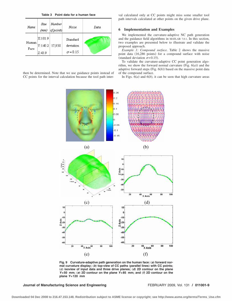
Fig. 9 Curvature-adaptive path genermal curvature display; „b… top-view of„c… isoview of input data and three drY=50 mm; „e… 2D contour on the plan
plane Y=120 mm


val calculated only at CC points might miss some smaller toolpath intervals calculated at other points on the given drive plane.

6 Implementation and ExamplesWe implemented the curvature-adaptive NC path generation

and the guidance field algorithms in MATLAB 7.0.1. In this section,two examples are presented below to illustrate and validate theproposed approach.

Example 1: Compound surface. Table 2 shows the massivepoint data �16,286 points� for a compound surface with noise�standard deviation �=0.15�.

To validate the curvature-adaptive CC point generation algo-rithm, we show the forward normal curvature �Fig. 6�a�� and theadaptive forward steps �Fig. 6�b�� based on the massive point dataof the compound surface.

In Figs. 6�a� and 6�b�, it can be seen that high curvature areas

(b)

(d)

(f)

n on the human face: „a… forward nor-paths „parallel lines… with CC points;planes; „d… 2D contour on the plane=85 mm; and „f… 2D contour on the

atioCCivee Y

FEBRUARY 2009, Vol. 131 / 011001-9


hca=ts

d „

0

Downloa

ave smaller forward steps. Figures 6�d�–6�f� further illustrate theurvature-adaptivity and the effect of the guidance field for pathst three different drive planes �Y =50 mm, Y =85 mm, and Y120 mm� where the distribution of the CC points is adaptive to

he local curvature, and the resulting paths are accurate even at aharp transition.

In our algorithm, we also achieve curvature-adaptive tool path

(a)

Fig. 10 Self-updating search bound inof the bound self-updating process an

Fig. 11 Curvature-adaptive tool pathgeneration from point data and „b… d
adaptive tool path intervals
11001-10 / Vol. 131, FEBRUARY 2009


intervals. Furthermore, we use guidance points to calculate thetool path intervals instead of CC points. As shown in Fig. 7, thelarge side normal curvature corresponds to the small tool pathintervals. Note that the dense tool path intervals also happens atthe regions with a high slope in the side direction.

We also use the synthetic data with high noise �standard devia-tion �=0.6� to illustrate MLS’s noise-handling ability. In Fig.

(b)

e guidance field algorithm: „a… displayb… zoom-in of the frame in „a…

a)

(b)rvals of the human face: „a… CC path

lay of the side normal curvature and

th

(

inteisp



8ti

��

c9a

s1ddrttQfifiioc

fatTawfi

7

t

Fchamr

J

Downloa

�a�, we can find noisy data. By projecting the input points ontohe MLS surface, we can see that the resulting compound surfaces much smoother �Fig. 8�b�–8�d��.

Example 2: Human face. Table 3 shows the massive point data17,938 points� for a human face with noise �standard deviation=0.15�.The forward normal curvature is displayed in Fig. 9�a�, and the

orresponding curvature-adaptive forward steps are shown in Fig.�b�. Three paths are shown to illustrate the curvature-adaptivitynd the guidance field effect �Figs. 9�c�–9�f��.

In our approach, we use the guidance field algorithm with theelf-updating bound to guarantee the machining accuracy. Figure0 presents a snapshot of how the guidance field works for therive plane in Fig. 9�d�. The small points stand for the input pointata and the big ones are the adaptive CC points. The circlesepresent the self-updating search bounds. As in Fig. 10�b�, Qj ishe current CC point, so based on its forward normal curvature,he next CC point should be point Qj+1� . However, between Qj and

j+1� , there exists a point with a larger normal curvature, so thenal forward step shrinks and a correct CC point Qj+1 is identi-ed. The results in Figs. 6 and 9 both demonstrate that the result-

ng paths are both curvature-adaptive and accurate due to the usef the guidance field algorithm. Figure 11 presents the resultingurvature-adaptive tool path intervals.

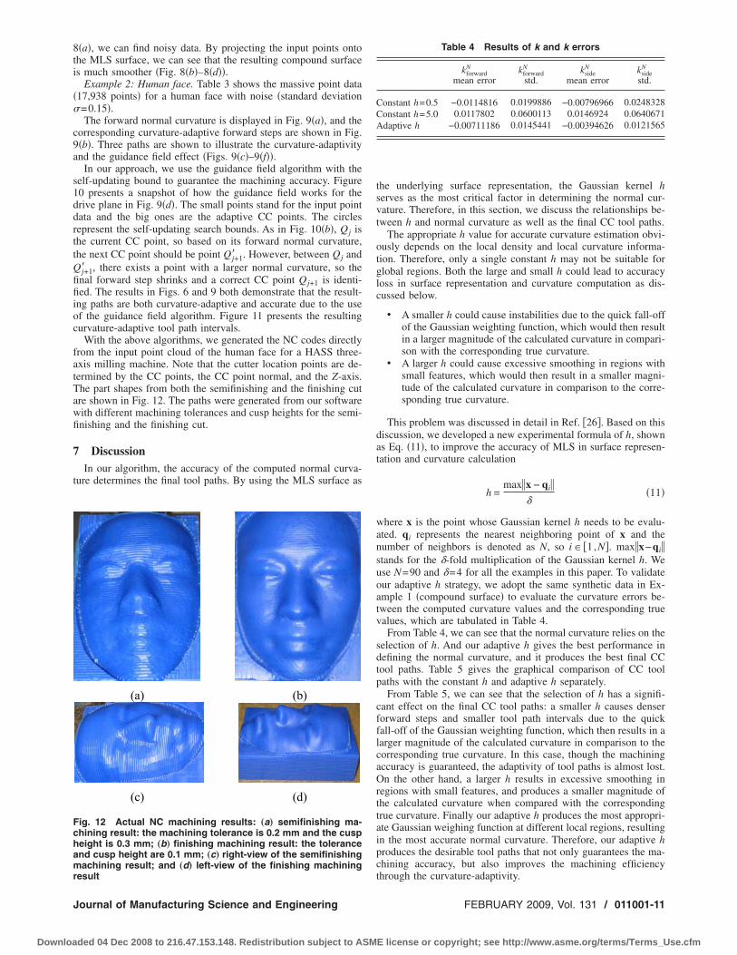
With the above algorithms, we generated the NC codes directlyrom the input point cloud of the human face for a HASS three-xis milling machine. Note that the cutter location points are de-ermined by the CC points, the CC point normal, and the Z-axis.he part shapes from both the semifinishing and the finishing cutre shown in Fig. 12. The paths were generated from our softwareith different machining tolerances and cusp heights for the semi-nishing and the finishing cut.

DiscussionIn our algorithm, the accuracy of the computed normal curva-

ure determines the final tool paths. By using the MLS surface as

(a) (b)

(c) (d)

ig. 12 Actual NC machining results: „a… semifinishing ma-hining result: the machining tolerance is 0.2 mm and the cuspeight is 0.3 mm; „b… finishing machining result: the tolerancend cusp height are 0.1 mm; „c… right-view of the semifinishingachining result; and „d… left-view of the finishing machining

esult



the underlying surface representation, the Gaussian kernel hserves as the most critical factor in determining the normal cur-vature. Therefore, in this section, we discuss the relationships be-tween h and normal curvature as well as the final CC tool paths.

The appropriate h value for accurate curvature estimation obvi-ously depends on the local density and local curvature informa-tion. Therefore, only a single constant h may not be suitable forglobal regions. Both the large and small h could lead to accuracyloss in surface representation and curvature computation as dis-cussed below.

• A smaller h could cause instabilities due to the quick fall-offof the Gaussian weighting function, which would then resultin a larger magnitude of the calculated curvature in compari-son with the corresponding true curvature.

• A larger h could cause excessive smoothing in regions withsmall features, which would then result in a smaller magni-tude of the calculated curvature in comparison to the corre-sponding true curvature.

This problem was discussed in detail in Ref. �26�. Based on thisdiscussion, we developed a new experimental formula of h, shownas Eq. �11�, to improve the accuracy of MLS in surface represen-tation and curvature calculation

h =max�x − qi�

�11�

where x is the point whose Gaussian kernel h needs to be evalu-ated. qi represents the nearest neighboring point of x and thenumber of neighbors is denoted as N, so i� �1,N�. max�x−qi�stands for the -fold multiplication of the Gaussian kernel h. Weuse N=90 and =4 for all the examples in this paper. To validateour adaptive h strategy, we adopt the same synthetic data in Ex-ample 1 �compound surface� to evaluate the curvature errors be-tween the computed curvature values and the corresponding truevalues, which are tabulated in Table 4.

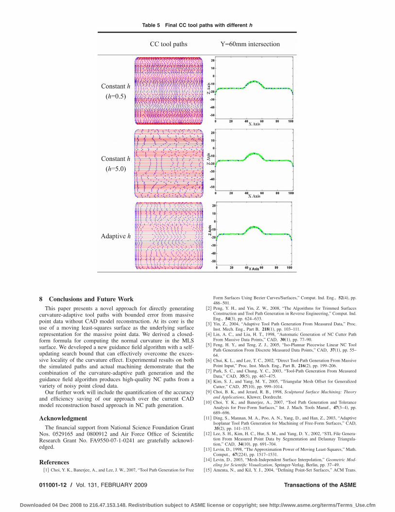
From Table 4, we can see that the normal curvature relies on theselection of h. And our adaptive h gives the best performance indefining the normal curvature, and it produces the best final CCtool paths. Table 5 gives the graphical comparison of CC toolpaths with the constant h and adaptive h separately.

From Table 5, we can see that the selection of h has a signifi-cant effect on the final CC tool paths: a smaller h causes denserforward steps and smaller tool path intervals due to the quickfall-off of the Gaussian weighting function, which then results in alarger magnitude of the calculated curvature in comparison to thecorresponding true curvature. In this case, though the machiningaccuracy is guaranteed, the adaptivity of tool paths is almost lost.On the other hand, a larger h results in excessive smoothing inregions with small features, and produces a smaller magnitude ofthe calculated curvature when compared with the correspondingtrue curvature. Finally our adaptive h produces the most appropri-ate Gaussian weighing function at different local regions, resultingin the most accurate normal curvature. Therefore, our adaptive hproduces the desirable tool paths that not only guarantees the ma-chining accuracy, but also improves the machining efficiency

Table 4 Results of k and k errors

kforwardN

mean errorkforward

N

std.kside

N

mean errorkside

N

std.

Constant h=0.5 −0.0114816 0.0199886 −0.00796966 0.0248328Constant h=5.0 0.0117802 0.0600113 0.0146924 0.0640671Adaptive h −0.00711186 0.0145441 −0.00394626 0.0121565

through the curvature-adaptivity.

FEBRUARY 2009, Vol. 131 / 011001-11


8

cpurfsustcgv

am

A

NRe

R

0

Downloa

Conclusions and Future WorkThis paper presents a novel approach for directly generating

urvature-adaptive tool paths with bounded error from massiveoint data without CAD model reconstruction. At its core is these of a moving least-squares surface as the underlying surfaceepresentation for the massive point data. We derived a closed-orm formula for computing the normal curvature in the MLSurface. We developed a new guidance field algorithm with a self-pdating search bound that can effectively overcome the exces-ive locality of the curvature effect. Experimental results on bothhe simulated paths and actual machining demonstrate that theombination of the curvature-adaptive path generation and theuidance field algorithm produces high-quality NC paths from aariety of noisy point cloud data.

Our further work will include the quantification of the accuracynd efficiency saving of our approach over the current CADodel reconstruction based approach in NC path generation.

cknowledgmentThe financial support from National Science Foundation Grant

os. 0529165 and 0800912 and Air Force Office of Scientificesearch Grant No. FA9550-07-1-0241 are gratefully acknowl-dged.

eferences

Table 5 Final CC too

�1� Choi, Y. K., Banerjee, A., and Lee, J. W., 2007, “Tool Path Generation for Free

11001-12 / Vol. 131, FEBRUARY 2009


Form Surfaces Using Bezier Curves/Surfaces,” Comput. Ind. Eng., 52�4�, pp.486–501.

�2� Peng, Y. H., and Yin, Z. W., 2008, “The Algorithms for Trimmed SurfacesConstruction and Tool Path Generation in Reverse Engineering,” Comput. Ind.Eng., 54�3�, pp. 624–633.

�3� Yin, Z., 2004, “Adaptive Tool Path Generation From Measured Data,” Proc.Inst. Mech. Eng., Part B, 218�1�, pp. 103–111.

�4� Lin, A. C., and Liu, H. T., 1998, “Automatic Generation of NC Cutter PathFrom Massive Data Points,” CAD, 30�1�, pp. 77–90.

�5� Feng, H. Y., and Teng, Z. J., 2005, “Iso-Plannar Piecewise Linear NC ToolPath Generation From Discrete Measured Data Points,” CAD, 37�1�, pp. 55–64.

�6� Chui, K. L., and Lee, T. C., 2002, “Direct Tool-Path Generation From MassivePoint Input,” Proc. Inst. Mech. Eng., Part B, 216�2�, pp. 199–206.

�7� Park, S. C., and Chung, Y. C., 2003, “Tool-Path Generation From MeasuredData,” CAD, 35�5�, pp. 467–475.

�8� Kim, S. J., and Yang, M. Y., 2005, “Triangular Mesh Offset for GeneralizedCutter,” CAD, 37�10�, pp. 999–1014.

�9� Choi, B. K., and Jerard, R. B., 1998, Sculptured Surface Machining: Theoryand Applications, Kluwer, Dordrecht.

�10� Choi, Y. K., and Banerjee, A., 2007, “Tool Path Generation and ToleranceAnalysis for Free-Form Surfaces,” Int. J. Mach. Tools Manuf., 47�3–4�, pp.689–696.

�11� Ding, S., Mannan, M. A., Poo, A. N., Yang, D., and Han, Z., 2003, “AdaptiveIsoplanar Tool Path Generation for Machining of Free-Form Surfaces,” CAD,35�2�, pp. 141–153.

�12� Lee, S. H., Kim, H. C., Hur, S. M., and Yang, D. Y., 2002, “STL File Genera-tion From Measured Point Data by Segmentation and Delaunay Triangula-tion,” CAD, 34�10�, pp. 691–704.

�13� Levin, D., 1998, “The Approximation Power of Moving Least-Squares,” Math.Comput., 67�224�, pp. 1517–1531.

�14� Levin, D., 2003, “Mesh-Independent Surface Interpolation,” Geometric Mod-eling for Scientific Visualization, Springer-Verlag, Berlin, pp. 37–49.

aths with different h
l p
�15� Amenta, N., and Kil, Y. J., 2004, “Defining Point-Set Surfaces,” ACM Trans.



J

Downloa

Graphics, 23�3�, pp. 264–270.�16� Amenta, N., and Kil, Y.-J., 2004, “The Domain of a Point Set Surface,” Eu-

rographics Symposium on Point-Based Graphics, pp. 139–147.�17� Alexa, M., Behr, J., Cohen-Or, D., Fleishman, S., and Levin, D., 2001, “Point

Set Surfaces,” Proceedings of the Conference on Visualization ‘01, SESSION:Session P1: Point-Based Rendering and Modeling, pp. 21–28.

�18� Dey, T. K., Goswami, S., and Sun, J., 2005, “Extremal Surface Based Projec-tions Converge and Reconstruct With Isotopy,” Technical Report No. OSU-CISRC-4–05–TR25.

�19� Dey, T. K., and Sun, J., 2005, “Adaptive MLS Surfaces for ReconstructionWith Guarantees,” Eurographics Symposium on Geometry Processing, pp. 43–52.

�20� Alexa, M., Behr, J., Cohen-Or, D., Fleishman, S., Levin, D., and Silva, C. T.,2003, “Computing and Rendering Point Set Surfaces,” IEEE Trans. Vis. Com-put. Graph., 9�1�, pp. 3–15.

�21� Scheidegger, C. E., Fleishman, S., and Silva, C. T., 2005, “Triangulating Point



Set Surfaces With Bounded Error,” Eurographics Symposium on GeometryProcessing, pp. 63–72.

�22� Hoppe, H., DeRose, T., Duchamp, T., McDonald, J., and Stuetzle, W., 1992,“Surface Reconstruction From Unorganized Points,” Comput. Graph., 26�2�,pp. 71–78.

�23� Pauly, M., 2003, “Point Primitives for Interactive Modeling and Processing of3D Geometry,” Ph.D. thesis, Computer Science Department, ETH Zurich.

�24� Goldman, R., 2005, “Curvature Formulas for Implicit Curves and Surfaces,”Comput. Aided Geom. Des., 22�7�, pp. 632–658.

�25� Yang, P., and Qian, X. P., 2008, “Adaptive Slicing of Moving Least SquaresSurfaces: Toward Direct Manufacturing of Point Set Surfaces,” ASME J.Comput. Inf. Sci. Eng., 8�3�, p. 031003.

�26� Yang, P. H., and Qian, X. P., “Direct Computing of Surface Curvatures forPoint-Set Surfaces,” Proceedings of 2007 IEEE/Eurographics Symposium onPoint-Based Graphics (PBG), Prague, Czech Republic, Sept. 2007.

FEBRUARY 2009, Vol. 131 / 011001-13


Documents

Adaptive NC Path Generation From Massive Point Data With