Embed Size (px)
Citation preview

12TH ICCRTS “Adapting C2 to the 21st Century”
AmmoSIM – Ammunition Simulation for Front Line
and Command Units
Track: 7
Corresponding author: Dr. Robert S. Woodley
21st Century Systems, Incorporated www.21csi.com
199 East 4th St., Suite B Ft. Leonard Wood, MO 65473
(573) 329-8526 [email protected]
Mr. Joe Barker 21st Century Systems, Incorporated
www.21csi.com 199 East 4th St., Suite B
Ft. Leonard Wood, MO 65473 (573) 329-8526
Mr. Warren Noll 21st Century Systems, Incorporated
www.21csi.com 199 East 4th St., Suite B
Ft. Leonard Wood, MO 65473 (573) 329-8526

AmmoSIM – Ammunition Simulation for Front Line and Command Units
Abstract AmmoSIM is an intelligent agent-based urban tactical decision aid (UTDA) for platoon and company commanders tasked with planning and executing military operations in urban terrain (MOUT). It is intended to provide warfighters with a tool to simulate and validate targeting effects in an urban terrain environment on the battlefield. Using accessed data from existing (and planned) terrain and tactical battlefield C2 sources and feeds, AmmoSIM calculates the ballistic trajectory of a given munition and models the effects on the target and surrounding area on the fly. AmmoSIM depicts the trajectory of weapons via a “virtual guidance Circular Error Probable (CEP)” in a linked 2D/3D view. The virtual guidance CEP is produced by combining sensor, munitions, and shooter characteristics in conjunction with calculations based on the targeting models from the Joint Technical Coordinating Group for Munitions Effectiveness (JTCG/ME). It allows the user to consider path obscuration or obstruction to the intended target, and weapon effects on known structure types using rubble generation algorithms. The intended result is to enable warfighters to more accurately predict where directed fires will hit and alert them to possible obstructions and structures or areas that war planners do not want hit based on the rules of engagement.
1. Introduction The development of AmmoSIM was initiated after experts shared their lessons learned from joint urban operations in Afghanistan and Iraq that there is a pressing need for tools to measure precision munitions use against small, fleeting, and concealed targets with minimal collateral damage. Commanders need graphical lethality and vulnerability analysis tools to support their requirements in considering the short- and long-term effects of firepower on the population, the infrastructure, and subsequent missions. Similarly, there is a need for a capability that provides immediate and accurate response fires. These observations were taken to mean accurate and measured fires must be simulated in a synthetic 3D urban terrain battlefield to minimize collateral damages and unintentional casualties.
AmmoSIM is an intelligent agent-based [A04, BN05] urban tactical decision aid used by platoon, company, and battalion commanders to simulate and validate targeting effects during combat operations in urban terrain. In a near real-time simulated environment, AmmoSIM simulates the direct employment and secondary effects of tanks, howitzers, and mortars against a given target(s) and the target area. It depicts the trajectory of these weapons in a 2D/3D view. AmmoSIM calculates the ballistic trajectory of given munitions and models the effects on the target and surrounding area as it uses accessed data from planned terrain and tactical battlefield command and control sources. Commanders must increasingly plan MOUT actions in an environment where there is miniscule, if any, room for error. AmmoSIM provides recommended courses of action that enhance currently fielded situational awareness systems for planners and decision makers [NWB06].
AmmoSIM utilizes typical GIS data to represent urban terrain in 2D/3D view. The user has the ability to define area(s) of interest (AOI). Forces, both friendly and non-friendly, along with targets are depicted in both textual and graphically in the 2D/3D views. Intelligent agents are utilized for such things as recommendations for firing solutions and limiting choices for target-shooter pairings. A first order rubble model has been developed for the prediction and display of rubble produced from target-shooter pairings. The statistical model utilized for firing solutions provides real time analysis of target-shooter pairings based upon the Physical Model Knowledge Acquisition Document (PKAD), U.S. Army Materiel Systems Analysis Activity (AMSAA).
Future planned development of AmmoSIM will include such things as use of the World Wide Construction Database, rubble model to include a wide array of building types and materials, plume modeling based upon accepted common standards and tools, seamless interaction with GIS data utilized

in the field such as the DTSS, and continual updating of military positions and targeting with wireless connections to C2. With a fully developed rubble model, AmmoSIM will be able to predict collateral damage, size and shape of rubble, and statistical analyses for specified kill types for target. Further development will enhance the 2D/3D views to utilize data supplied from typical GIS repositories with synthetic 3D urban terrains depicted on the fly. In the field, collaboration will allow for common viewing of the Military Operations in the Urban Terrain (MOUT). Collaboration would enhance planning and situational awareness for platoons and C2.
2. AmmoSIM methodology and base functionality In order to tailor AmmoSIM to meet prospective users’ needs, the rapid application development (RAD) approach applied was to demo the work-in-progress prototype and gather comments from working groups and conferences. This put the AmmoSIM team in direct contact with possible users and customers, allowing them to quickly transition gathered knowledge into the product. These groups include:
• Joint Technical Coordinating Group for Munitions Effectiveness (JTCG/ME) • Army Material Systems Analysis Activity (AMSAA) • Joint Munitions Effectiveness Manual Surface-to-Surface (JMEM/SS) Operational Users
Working Group (OUWG) • Joint Technical Coordinating Group for Munitions Effectiveness (JTCG/ME) Operational Tools
and Methodology Standardization (OTMS) • Urban Operations Summit
The base AmmoSIM functionality comes from two paradigms: First, AmmoSIM uses a mathematical/statistical approach to calculating the various components of the system as opposed to brute force (table-based) methods that are currently used in the field. Second, the calculations developed can be utilized for single engagements or, in what is known as barrage mode, AmmoSIM creates a simulated multi-shot volley to show what is likely to occur in an engagement. 2.1. Ballistics and error calculations - Incorporating JMEMs Data Access to JMEMs data was intended to allow 21CSI to incorporate real weapons data in the single shot and barrage mode calculations. JMEM data was reviewed and extensive research was performed along with discussions with JTCG/ME about the development of the JWS API (available mid 2007). The JMEM data is classified and to keep the AmmoSIM project unclassified, it was decided to utilize only unclassified data. Weapon accuracy was determined from a document from AMSAA that provided real world weapons processes [PKAD04].
2.1.1. Impact Location Error As described in the PKAD document, indirect weapons fire accuracy is dependent on a number factors including targeting method, system and munition types, and range. Most of these factors and their results are commonly organized into tabular form (See Table 1 for a constructed example). The targeting method is treated separately as a classification matching type to standard deviation of error (or similarly, circular error probable, CEP). Table 1: Example (constructed) weapon accuracy table
System/Weapon/Mount Munition Range (m)
PE Range Error σ
PE Deflection Error σ
MPI Range Error σ
MPI Deflection Error σ
(SP Howitzer) A 6257 23.2 7.1 48.1 37.3 (SP Howitzer) A 12111 28.7 8.9 83.4 61.8 (SP Howitzer) A 18009 53.2 18.8 128.6 115.4 (Mortar) B 101 0.4 0.1 0.8 0.6 (Mortar) B 1557 3.7 1.1 10.7 7.9 (Mortar) B 3215 9.5 3.4 23.0 20.6
The ultimate result of the calculations discussed in the paper provides the standard deviations of the Impact Location Range (ILR) and Impact Location Deflection (ILD). It is assumed that each process that leads to error itself has a normal distribution. Additionally, the processes are assumed to be additive. In other words, each source of error adds it’s offset to the others. Given these assumptions, the overall standard deviations can be calculated as follows:
Κ++= 22
21 σσσTOT
Specifically, for ILR:
222 )()()( RangeRangeILR PEMPITLE ++= σσ
• TLE BσB=standard deviation of Target Location Error (based on targeting method) • MPI BRangeB=Mean Point of Impact in the “range” direction (interpolated from table) • PE BRangeB=Precision Error in the “range” direction (interpolated from table)
Similarly, σBILDB is calculated using the same TLEBσ B, but substituting MPIBDeflectionB and PEBDeflectionB. It should be noted that while these formulas are useful for simulating impact locations, they only indirectly indicate the accuracy [NKNW96].
2.1.2. Impact Accuracy In order to convert the previously calculated standard deviations into a usable accuracy value, we must utilize the normal distribution functions. Specifically, a bivariate normal distribution is most appropriate since both σBILRB and σBILDB are orthogonal and normal. Given the distribution and its parameters (σBILRB, σBILD B), we wish to determine the probability that the shell will land within a given shape (building outline, circle, etc.).
The easiest calculation, and therefore the one we will start with, is that of a square aligned to the range and deflection axes. This is quite simple because we know that each axis consists of a normal distribution, therefore, the probability that a shot will land in the square with corners (x B1B,y B1B) and (xB2B,y B2B) is:
⎥⎦
⎤⎢⎣
⎡⎟⎟⎠
⎞⎜⎜⎝
⎛−⎟⎟
⎠
⎞⎜⎜⎝
⎛⋅⎥
⎦
⎤⎢⎣
⎡⎟⎟⎠
⎞⎜⎜⎝
⎛−⎟⎟
⎠
⎞⎜⎜⎝
⎛=
ILRILRILDILDhit
yFyFxFxFPσσσσ
1212
(where F(z) is the standard normal cumulative distribution function)
A more difficult problem is to determine what possible chance there is for a shot to land within a certain distance of the target. In other words, given a circle drawn around the target, what percentage of the time should the shot land inside it. This would be difficult problem and we would have to resort to numerical integration if not for the realization that the standard bivariate normal distribution is radially symmetric. That is, the distance from the central (target) point alone determines the chance to hit and the bearing is unimportant. However we still require a rigorous proof for it to be trusted:
( )2
21
21 z
ezf−
=π
(Standard normal pdf)
( ) ( ) ( )2121, zfzfzzf ⋅= (Standard bivariate normal pdf) Now perform a change of variables to polar coordinates:
( ) ( ) ( )
( ) ( )[ ] ( ) ( )
( )rf
eee
eerrf
rrrr
rr
π
πππ
ππθθ
θθθθ
θθ
21
21
21
21
21
21)cos(),sin(
121)(cos)(sin
21)cos()sin(
21
)cos(21)sin(
21
222222
22
=
⋅=⋅=⋅=
⎟⎟⎠
⎞⎜⎜⎝
⎛⋅⎟⎟
⎠
⎞⎜⎜⎝
⎛=⋅⋅
−+−⋅+⋅−
⋅−⋅−

Thus proving not only that the standard bivariate normal distribution is radially symmetric, but also that it is directly proportional to the distance from the central point [NKNW96]. (Note that we get another bonus from this symmetry because we can remove the “alignment” constraint from the previous problem, since we can rotate any rectangular shape to appear aligned without altering the results.)
We next seek to find the radial cdf (cumulative distribution function):
( ) ( )
( )
( ) ( )∫∫∫
∫ ∫
∫ ∫
⋅⋅=⋅⋅⋅=
⋅⋅=
⋅⋅⋅⋅=
rr
r
r
zz
z
z
r
drrfrdrrfrd
ddrrrf
ddrrrrfzF
00
2
0
2
0 0
2
0 0
221
21
)cos(),sin(ˆ
πθπ
θπ
θθθ
π
π
π
This results in an integral that, just as its cousin, has no closed form and must be approximated. However, instead using a generic numerical solver, we can create a more clever approximation. When applying integration by parts multiple times, a pattern emerges:
( ) ( )
( ) ( )
( ) ( ) ( )
( ) ( ) ( ) ( )
( ) ( )∫∑
∫
∫
∫
∫
⋅⋅
+⋅
⋅=
⋅+⎥⎦⎤
⎢⎣⎡+⎥⎦
⎤⎢⎣⎡+⎥⎦
⎤⎢⎣⎡=
⋅+⎥⎦⎤
⎢⎣⎡+⎥⎦
⎤⎢⎣⎡=
⋅+⎥⎦⎤
⎢⎣⎡=
⋅=
+
=
r
r
r
r
r
z nn
n
i
irir
z
rrrrrr
z
rrrr
z
rr
z
r
drrfrn
zi
zf
drrfrzfzzfzzfz
drrfrzfzzfz
drrfrzfz
drrfrzF
0
12
1
2
0
7642
0
542
0
32
0
!21
!21
481
481
81
21
81
81
21
21
21
ˆ21π
If we examine the integral term, we see that as n grows large the exponent and factorial terms drive the integral to zero as they overwhelm the power term (the f term remains constant). So, for large enough n, we can neglect the integral giving:
( ) ( ) ∑∞
= ⋅⋅⋅=
1
2
!212ˆ
i
irirr z
izfzF π
This is easily approximated in software.
With this in hand, we can determine the hit ratio inside a circle of given radius. While this is useful, it is much more likely that we would wish to know the inverse problem. That is, what is the circular error for any given probability? The simplest solution is a brute force binary search, requiring a number of evaluations of the previous function on the order of the number of bits of precision required. Though accurate, this can be slow. In order to generate the required values in a timely manner, a curve fit function was generated. This function provided accuracy on the order 10-6 for any percentage less than 99.75%. For percentages greater than this, the curve’s error grows significantly. In these cases, the slower algorithm is used. 2.2. Design & Develop Barrage Mode Barrage mode in AmmoSIM is essentially the multi-shot extension of its single shot mode. This allows scenarios and experiments to be conducted to determine the best set of assets to use against a given target along with the amount of time/munitions required to destroy it. Much of this is dependent on the rubble model described below and the accuracy calculations described above.

2.2.1. Statistical model for multi-shot The accuracy calculations give the ability to determine a “percent hit” value. Determining the various statistics of a multi-shot attack then becomes simple with the realization that this pattern will match the binomial distribution. That is, since each event (shot) has a yes or no outcome (“hit” or “no hit”), we can use the binomial distribution as a model for barrage mode.
The binomial distribution takes this form:
( ) ( ) knk ppkn
pnkf −−⋅⋅⎟⎟⎠
⎞⎜⎜⎝
⎛= 1,;
Given n, the number of tries, and p, the chance of success, what is the chance of having exactly k successes?
It can easily be seen how closely this fits the barrage operation. Various other questions can also be answered by applying the appropriate statistical operations. For instance, we normally wish to know the odds for at least some number of hits instead of exactly some number. To calculate this simply involves the sum over the desired range of acceptable hit count. Answering the reverse question is also possible. That is, how many shots must be fired to ensure at least some number of hits occurs? This, of course, requires an inverse function. While somewhat computationally expensive, this value is also easily determined. In general, it can be seen that this model both closely matches the original process and can answer any useful question the user/operator may need to know.
3. AmmoSIM rubble modeling Rubble impacts mission accomplishment, particularly in the area of movement and maneuver. It is important to adequately model rubble generation from fires activities in order to predict the ability of a vehicle to override the collateral damage from weapon effects in urban areas. The US Army Modeling and Simulation Office (AMSO) have done some research into munitions effects, cratering, and urban debris. They have also done some research into vehicle performance in the face of urban debris and cratering. This research was conducted under its Military Operations in Urban Terrain Focus Area Collaborative Team (MOUT FACT).
The development of a robust rubble characterization model is a very complicated problem if all aspects of building collapse and rubble generation are to be considered and characterized in their entireties. To bind the problem and render it tractable, a number of simplifying assumptions have been made. The model presented herein considers only thick uniform masonry buildings with square or near-square footprints. In addition, the model only considers ground-based directed weapons fire, and not blast loads or placed charges since guidelines for building demolition using placed charges are already readily available. The model does not consider armor-piercing projectiles because their primary effect upon impacting the wall of a building is to put a hole in that wall.
Two types of models are developed: a first-order model and a first-principles-based model. In both models, we assume complete rubblization of the building and develop a rubble profile model using the size and composition of the collapsed structure to predict the rubble volume. In both cases, this profile model includes the size of footprint area surrounding original building assuming that the rubble is free to expand horizontally as well as the resulting height of such a rubble pile. The height of rubble pile along its periphery is adjusted based on the proximity of other buildings. These adjacent buildings will be assumed to block rubble dispersion, thereby forcing it to back-fill or stack up along the edges of the adjacent buildings that face the center of the collapsed building site.
For the purposes of this study, we assume that the building is without a basement and that it is located in a residential area. It is presumed not to be an office building or a building in a shopping district with significant glazing facing the street. The major effect of whatever windows do exist is to reduce the amount or volume of building material; this effect is introduced through a volume reduction factor of

some nominal amount. Figure 1 below presents a sketch of a generic building illustrating a nearly square footprint area.
L
H
D
L
H
D
Figure 1: Sketch of Generic “Boxy” Building
In order to determine the dimensions of the rubble pile following building collapse, we need to know the values of the following geometric parameters: L, the length when looking straight at building from firing location; D, the depth of building along line of fire; H, the building height; NBSB, the number of stories in building; NBRB = NBRLBxNBRDB, the number of rooms per story (assumed equal for all stories), where NBRLB is the number of rooms along the length of the building and NBRDB is the number of rooms in the building depth direction; tBwe B, the exterior wall thickness (assumed equal for all exterior walls); tBwiB, the interior wall thickness (assumed equal for all interior walls); tBfe, Bthe floor thickness (assumed equal for all floors); t Br B, the roof thickness; d Bb B, the basement depth. Other information that is required to develop the rubble pile model is building material properties, the proximity of other buildings to the building of interest, and the weight or energy of explosive used to demolish the building. 3.1. Initial Calculations The first step in calculating the dimensions of the rubble pile is calculating the volume of building material in its upright or functional configuration. This building material volume is given as follows:
Building material volume = volume of 4 exterior walls + volume of (N BSB-1) floors + volume of (NBRLB-1) interior walls parallel to line of fire + volume of (N BRDB-1) interior walls perpendicular to line of fire + volume of roof (1)
These quantities are given as follows. Roof Volume VBr B= LDt Br (2)
Exterior walls (4) volume VBwe B = 2L(H-t Br B)t Bwe B+2D(H-t Br B)t Bwe (3) Volume of NBs B-1 floors VBfl B= (NBs B-1) (L-2t Bwe B) (D-2t Bwe B) t Bfl (4)
The volume of the N BRLB-1 interior walls along line of fire is given by VBWRLB=Ns x h BLB x dBDB x (NBRLB-1) x NBRDB x t Bwi (5)
where h BL Bis the wall height and dBD Bis the wall depth along the line of fire. These quantities are given as follows:
h BLB= [H-tr-(NBs B-1)t BflB] / NBs (6) d BDB=[D-2tBwe B-(NBRDB-1)t Bwi B] / NBRD (7)
Finally, the volume of NBRDB-1 interior walls across the line of fire is given by VBWRDB=NBs Bx (NBRDB-1) x NBRL Bx hBL Bx B Bd BL Bx t Bwi (8)
where h BL Bas before and d BLB=[L-2tBwe B-(NBRLB-1)t Bwi B] /NBRL (9)
In the following analysis, we assume that the rubble pile is in the shape of a right circular cone centered about the geometric center of the original building.

3.2. First-Order Model In developing a first-order model of the rubble pile, we postulate that the radius of the cone is twice that of the building’s average floor half-length. This assumption is consistent with photographic and empirical evidence obtained at building collapse sites. For example, Yarimer and Brown [YB96] postulate that as a “collection of blocks falls, it creates a pile of rubble of height αΔh, where Δh is the intact structure height converted into rubble.” They subsequently use a value of α=0.15 to fit their analyses to their experimental data. A simple calculation equating the volume of an H x L x D block to that of a cone having a base radius r Bc B and a height of 0.15H yields the result that r Bc B = 2.52L (assuming that D and L are comparable in size, as we are doing in this study).
Mathematically then, we have that the rubble cone radius is given by
r Bc B = 12
x avg(L,D) x 2 (10)
The height of the debris pile is then calculated from
VBtot B= 3π (rBc PB2 P) h Bc (11)
where VBtotB = VBr B+ VBwe B+ VBfl B+VBWRL B+ VBWRD (12)
We note that the total volume V BtotB is multiplied by a bulk-up factor and a window effects factor to account for the bulking up in apparent volume that typically occurs when a compact object is exploded and for the reduction in volume due to the presence of windows in the building of interest. The actual extent of the rubble debris pile will depend on the proximity of the buildings adjacent to or across the street from the collapsed building. If the rubble pile created would normally extend beyond the distance to the closest building (i.e. if the adjacent building were not there), then it is presumed that the rubble pile will “stack up” next to the adjacent building and a heightening of the rubble would occur near the adjacent building.
If we let DBSB be the distance between the original building and the closest adjacent building, then back-filling would occur if and only if
12
x avg(L,D) + DBSB U>U r Bc (13)
If we let Δ denote the extent beyond the façade of the adjacent building that the rubble would extend if there were no adjacent building, then the height of the backfilled material next to the adjacent building is calculated as follows.
First, we need to calculate the amount or volume of material that is allowed to “stack up” on top of the original cone volume due to the presence of an adjacent building. Referring to XFigure 2 X below, AEO is a line running through the geometrical center of the original (upright) building, while DB is the façade of an adjacent building. Line ABC rests on street level.
O
E D
CBAS
1 x (L,D) + D2
avg Δ
cr
ch
O
E D
CBAS
1 x (L,D) + D2
avg Δ
cr
ch
Figure 2: Geometrical Considerations for Calculating Back-fill Volume VBBCDB
In this case, the volume of material in the annular cone defined by triangle BCD is the amount of material that stacks up next to the adjoining building, creating this back-fill effect. Using similar triangles, this volume is found to be given as follows.
VBBDCB = 3π r Bc PB2Ph Bc B- 3
π [ 12
x avg(L,D) + D BSB]P2 P{h Bc B- c
c
hr
[r Bc B– ( 12
x avg(L,D) + D BSB)]} - π [ 12
x avg(L,D)
+ DBSB]P2 P{r Bc B – [ 12
x avg(L,D) + DBSB]} (14)
where r Bc B and h BcB are given by equations X(10)X and X(11)X, respectively.
The next step is to calculate the new profile of the rubble pile due to this back filling of debris material next to the adjacent building. Referring to XFigure 3X below, this amounts to calculating distance DD’. For the purposes of this model, the back-filling is assumed to occur linearly from the façade of the adjacent building back to the tip of the cone defining the original debris pile.
O
E D
CBAS
1 x (L,D) + D2
avg Δ
cr
D’E’ch
O
E D
CBAS
1 x (L,D) + D2
avg Δ
cr
D’E’ch
Figure 3: Geometrical Considerations for Calculating Stack-up Height DD’
We find DD′ by noting that the volume of material in the new configuration equals the original volume of cone OAC, or that the volume of cone OAC equals the volume of cone OE’D’ plus the volume of cylinder E’ABD’:
3π r Bc PB2Ph BcB =
3π (E′D′) P2 P(E′O) + π (AB)P2 P(BD′) (15)
Again, using similar triangles and other fundamental relationships between the various geometric shapes in Figure 3, we solve for DD′ with the result:
2c c
2c
S
h rDD' = - (1+2 )
2 r1 x avg(L,D) + D2
⎧ ⎫⎪ ⎪Δ⎪ ⎪⎨ ⎬
⎡ ⎤⎪ ⎪⎢ ⎥⎪ ⎪⎣ ⎦⎩ ⎭
(16)
where Δ is given by
Δ = r Bc B – [ 12
x avg(L,D) + DBSB] (17)
and length BD is given by
BD = ( c
c
hr
) Δ (18)
3.3. First-Principles-Based Model In the previous section, a first-order model of the rubble pile that is created following building collapse was developed. In the model to be developed in this section, we use the principle of energy conservation to remove this assumption and use a first principles calculation to determine the horizontal extent of the rubble pile. Simply put, we have:

Explosive energy = Fragmentation of roof + Fragmentation of ceilings/floors + Fragmentation of all walls + Fragmentation of floor (lowest) + Motion of roof + Motion of ceilings/floors + Motion of walls + Motion of floor (lowest) (19)
To be conservative, we assume that all of the explosive energy goes into debris movement; none of it gets applied to fragmentation or debris formation. This should result in more widespread debris, which should render the model more conservative in nature. Furthermore, we assume that the building’s roof and its ceilings/floors fall straight down and that their debris do not travel outward out (debris from the building’s lowest floor is presumed to remain where created). In addition, for this model, we are neglecting lift and drag forces on the rubble pieces as they move through the air and consider only gravity effects. Under these assumptions, equation X(19)X reduces to
Explosive energy = Energy of motion of all walls (20) In a building that is N Bs B stories high and has NBRB = NBRL Bx NBRDB rooms, the number of walls is found by adding the number of exterior and interior walls as follows:
NBwB = NBw,extB + NBw,intB (21) where
NBw,ext B= 2 x NBS Bx NBRL B+ 2 x NBS Bx NBRDB (22) and
NBw,int B = NBs B x NBRL Bx (NBRD B– 1) + NBs Bx (NBRLB – 1) x NBRDB (23)
In this model, we seek to bind the radius of the cone defining the rubble pile. To accomplish this, the focus of the calculations that follow will be on obtaining the distance traveled by a piece of rubble that is ejected from one of the highest external walls. Partitioning the energy of the explosion among all walls whose fragments are assumed to move yields the amount of energy available for any given wall:
EBavailB = EBexplB / NBwB (24) where the energy of the explosion, EBexplB, is given and NBwB is given by equations X(21)X, X(22)X and X(23)X. The next step is to determine the mass(es) and velocity(ies) of the particle(s) of interest.
To begin, we examine a possible path that could be followed by the center-of-mass of the rubble ejected from the highest wall of the building as shown in XFigure 4X below. In XFigure 4 X, MBcomB is the mass of the exterior room wall that has been rubblized, VBcomB is the velocity of the center-of-mass of the wall rubble, tBtopB is the time of travel to the highest point of the trajectory, tBgrB is the time required for the wall center-of-mass to reach the ground, and XBgrB is the distance from the building to the point at which the wall rubble center-of-mass reaches the ground.
time tgr
Mcom, Vcom
distance Xgr
?
time tgr
Mcom, Vcom
distance Xgr
?
Figure 4: Trajectory of Wall Section Rubble Center-of-Mass
Based on the definitions of MBcomB and VBcomB, we can also write, on a per-exterior-wall basis, [A99]
EBavail B= 12
MBcom BVP2 PB
comb (25)
Additionally, the mass of an exterior room wall, M BcomB, is given by

MBcom B= VBwe BρBwe B / NBw,extB (26) where ρBwe B is the density of the exterior wall material, and VBwe B and NBw,extB are given by equations X(3)X and X(22)X, respectively. Using equation X(25)X to solve for VBcomB yields
VBcomB = avail com2E / M (27)
where MBcomB is given by equation X(26)X.
We now know the velocity at which the center-of-mass of the rubble debris is assumed to travel until it hits the ground. In order to determine the location of ground impact, several intermediate quantities must be calculated.
First, the starting point (or height SBOB) of the trajectory shown in XFigure 4 X is needed. Referring to XFigure 5 X XbelowX, we see that:
O r w1S = H - t - h2
(28)
where h BwB is the floor-to-ceiling height of the exterior room wall.
H
tr
hw
H
tr
hw
Figure 5: Detail for Calculating Starting Height SBOB
Second, the travel time tBgr Bmust be found. From elementary physics, we recall that the relationship between free-fall distance S and the acceleration due to gravity ‘g’ is given by:
2
2
S gt
∂= −
∂ (29)
Integrating equation X(29)X twice and applying initial conditions of velocity and height yields 2
O com1S S V (sin )t gt2
= + θ − (30)
The time tBgr B at which the rubble debris center-of-mass hits the ground is found by setting S = 0 in equation X(30)X and solving for time ‘t’ to yield,
2com com O
gr
V sin (V sin ) 2gSt
gθ + θ +
= (31)
To maximize the horizontal distance traveled, the material needs to be ejected at an angle of / 4θ = π . With this value of θ, equation X(31)X becomes
2
com com Ogr
V V S2 2t ( ) 24 2 g 2 g g
⎡ ⎤⎛ ⎞ ⎛ ⎞ ⎛ ⎞πθ = = + +⎢ ⎥⎜ ⎟ ⎜ ⎟ ⎜ ⎟⎜ ⎟ ⎜ ⎟ ⎝ ⎠⎢ ⎥⎝ ⎠ ⎝ ⎠⎣ ⎦
(32)
Finally, the horizontal distance traveled at the time of impact given by equation X(32)X is simply the product of the horizontal component of the velocity of the rubble debris center-of-mass and the quantity tBgrB, or,
gr com grX =V cos t =4 4π π⎛ ⎞ ⎛ ⎞θ⎜ ⎟ ⎜ ⎟
⎝ ⎠ ⎝ ⎠ (33)
If a value of 0θ = were used instead of / 4θ = π , then t BgrB and XBgrB are given by

Ogr
St ( 0) 2
g⎛ ⎞
θ = = ⎜ ⎟⎝ ⎠
(34)
Ogr com
SX ( 0) V 2
g⎛ ⎞
θ = = ⎜ ⎟⎝ ⎠
(35)
3.4. Comparison of Model Predictions
Both of the models developed in this study were run for a four-story unreinforced concrete (density 145 lb/ftP3P) building with four rooms on each floor. The building was 22 ft high with 6 in. exterior walls, 3 in. interior walls, a 6 in. roof, and had a 20 ft x 21 ft footprint. A bulk-up factor of 1.5 and a window effects factor of 0.9 were used in the model calculations. Adjacent buildings were assumed to be 9 ft away from the outermost wall of the building of interest.
Although the rubble pile dimensions are independent of the weapon charge used to explode the building in the first-order model, the first-principles based model requires this information as input. For the engagement scenarios anticipated, charge-fills are expected to range from 0.5 kg = 1.1 lbs TNT for small mortars up to 10 kg = 22 lbs TNT for Howitzers. As such, a charge of 10 lbs TNT was selected for running the first-principles based model.
In order to run the first-principles model, the weight of the charge first had to be converted into an energy delivered. While there are several measures of explosive strength given the weight of a charge, to be conservative, a value of 0.8 x 10P6P J/kg (or 3.6 x 10P6 P J for 10 lbs of TNT) was used in this study [M795]. XTable 2 X below summarizes the main rubble pile characteristics produced by both models for the geometry, material, and loadings described. Table 2: Rubble Pile Dimensions as Calculated by Models
Rubble Pile Dimension
First-OrderModel
First-PrinciplesModel (θ=45P
oP)
First-Principles Model (θ=0P
oP)
Radius (rBc B), ft 20.5 50.8 42.6 Height (hBc B), ft 4.8 0.79 1.12 Stack-up Height (DD’), in 0.35 22.32 18.82
For the 10 lbs TNT charge considered, the first-principles based model clearly predicts a rubble pile radius far in excess of the first-order model. As expected, assuming a 45PoP trajectory for the rubble pile increased still further the distance traveled by the rubble center-of-mass. For larger charges, these discrepancies are further increased. Clearly, at this point, empirical data is needed to verify the predictive capabilities of these various models.
4. AmmoSIM advanced 3D display technology 4.1. Interface Development As with any decision-aid software, AmmoSIM is only as good as the data it works on. In this regard, we investigated interfacing to a number of data sources providing sever data types. Primary among the sources investigated is GIS, or Geospatial Information Systems. These systems provide access to a wealth of information ranging from satellite imagery to demographic data, street maps to coastal charts. This has been a rapidly growing segment in information systems and, as has happened before, interfacing with all the various industry standards can be difficult. To combat this, the Open Geospatial Consortium (OGC) created an open standard for geospatial information systems, OpenGIS. In order for AmmoSIM to be as compatible as possible, it was obvious that this standard needed to be supported. In order to accomplish this, a number of software tools were used. The open source toolkit GeoTools provides access methods to GIS primitives and an abstraction layer to the various GIS-compatible database

applications. MapServer and GeoServer (itself built with GeoTools) provide more indirect access to GIS data, specifically the Web Mapping Service (WMS) and Web Feature Service (WFS) feature sets. The WMS provides visual representations of GIS data using well known web data-access mechanisms. AmmoSIM, through AEDGE Map2D, utilizes WMS servers to organize and access large image sets such as satellite imagery. The WFS again uses well known web mechanisms to provide access to GIS features. These features include such items as geographic shapes with associated attributes in an XML format. In addition to these mechanisms defined by the OpenGIS standard, the use of the Commercial Joint Mapping Toolkit (C/JMTK) by AmmoSIM was also investigated. The C/JMTK is built from commercial GIS tools and is intended to provide a common GIS standard across the military.
Another source of data required for the functionality of AmmoSIM is the various weapon data. Two sources investigated were the Joint Weaponeering System (JWS) and NATO Armaments Ballistic Kernel (NABK). In order to provide rubble estimation capabilities, several toolkits were examined in addition to the rubble model detailed above. The two external toolkits were the Blast Effects Estimation Model (BEEM) and Structural Weapons Effects (SWE) API. The information gathered from this investigation proved useful in making AmmoSIM easily adaptable to new information sources [CZC01]. 4.2. Improve Visualization & Urban Representation
4.2.1. 3D Visualization In an effort to improve support for 3D applications, 21CSI utilizes an engine based on the Torque Shader Engine (TSE). Torque brings advanced high performance rendering techniques to the table, along with the quality of a Triple-A gaming engine. For example, Torque can automatically handle the problem of Level of Detail (LOD).
However, while the new 3D provided many benefits, it also introduced several complications. Due to its pedigree (gaming focus), it could not initially support a number of real world requirements. Game developers generally design static (or pre-scripted dynamic) environments and limit their own resource usage in order to guarantee solid, predictable performance. In other words, they will limit the number of objects and size of imagery in their scenes to ensure that good performance will be had on the target hardware platform. They have even gone so far as reshaping the landscape and placing obscuring objects in order to limit the total number of objects in view. In the real world, however, these assumptions and tricks are not possible. Users will expect performance even when extreme numbers of objects (buildings) and vast amounts of imagery (satellite) are accessed. The only saving grace is that real-world users tend to have lower absolute performance expectations than gamers, but they still require consistent performance.
These difficulties are not insurmountable, though. AmmoSIM can access and display features and imagery through GIS standard methods. XFigure 6X shows a 3D view of Baghdad utilizing real building shapes and real satellite imagery. It should be noted that these images are generated from data on a huge scale, over 100,000 buildings total and 1.5GB of satellite imagery.
Figure 6: 3D view of Baghdad
4.2.2. 2D Visualization 3D views of the battlefield are incredibly useful, however, additional views are also needed to fully convey the situation to the user. Since a great deal of the work AmmoSIM will help with was done on 2D paper maps, it was decided that a 2D “map” view was needed to enhance comprehension and ease the transition from 2D to 3D ways of thinking. The large number of (possibly) visible buildings and the size of the imagery requires care to display. In order to support the display of data sets with these issues, compatibility with the OpenGIS WMS was integrated to provide use of large imagery sets. The system also supports tiling and pyramiding (a form of Level of Detail) to improve performance and reduce resource requirements. The end result is a 2D map that can visualize large real-world data sets in conjunction with AmmoSIM primitives, such as the various zone shapes. An example of the 2D map is shown in XFigure 7 X

Figure 7: 2D view of Baghdad
4.3. Application of the rubble model in AmmoSIM There are two possible areas where AmmoSIM could apply the rubble model calculations. The first was implemented while the second was postponed due to technical limitations. The first application was the use of the rubble model to determine a percent kills value for given targets, ammunitions, weapons platforms, etc. This value is useful to the user on its own as well as helping to provide a recommended number of shots in barrage mode.
The second application was the actual display of a rubblized building. However, the 3D, being based on Torque with its background in gaming proved extremely difficult to modify, such as in breaking apart and displaying building models based on the rubble model calculations. Game engines are typically built with the assumption of static or semi-static terrain. While the modification is possible, the resource required were simply not available in the current effort. In lieu of this capability, AmmoSIM can display buildings in a whole or (precalculated) destroyed state. Example screenshots are provided in XFigure 8 X and XFigure 9 X.

Figure 8: Target Before Explosion
Figure 9: Target After Explosion

5. AmmoSIM prototype and results 5.1. Prototype Specification and Implementation This task involved bringing together all the work accomplished into one final product. The results were combined into the various design documents used in our development process:
• Software Requirement Specification • System/Subsystem Requirement • Software Design Document • Software Test Document/Plan
With these documents complete, development could begin. The development process made use of a number of notable tools, many open source. Primary among these is the Eclipse RCP development platform. Eclipse provides a host of tools, including an IDE, widget toolkit, plugin infrastructure and more. Eclipse provides native look and feel to Java applications with its SWT API, which interfaces directly with the native OS’ GUI functionality. Other open source tools used include Hibernate, for easy and flexible database access, and GeoTools, for OpenGIS compliant access and manipulation of geospatial data. 21CSI’s experience with developing decision support software allowed us to develop the prototype very rapidly [ECD00].
5.2. Results Figures 10 – 15 show the various screens from the AmmoSIM software and a brief description of what is shown.
Figure 10: Selected Target A selected target is highlighted and the camera positions to display the target.
Figure 11: Asset Target Pairing With a target asset pairing, the camera positions behind the asset in the direction of the target in the distance.
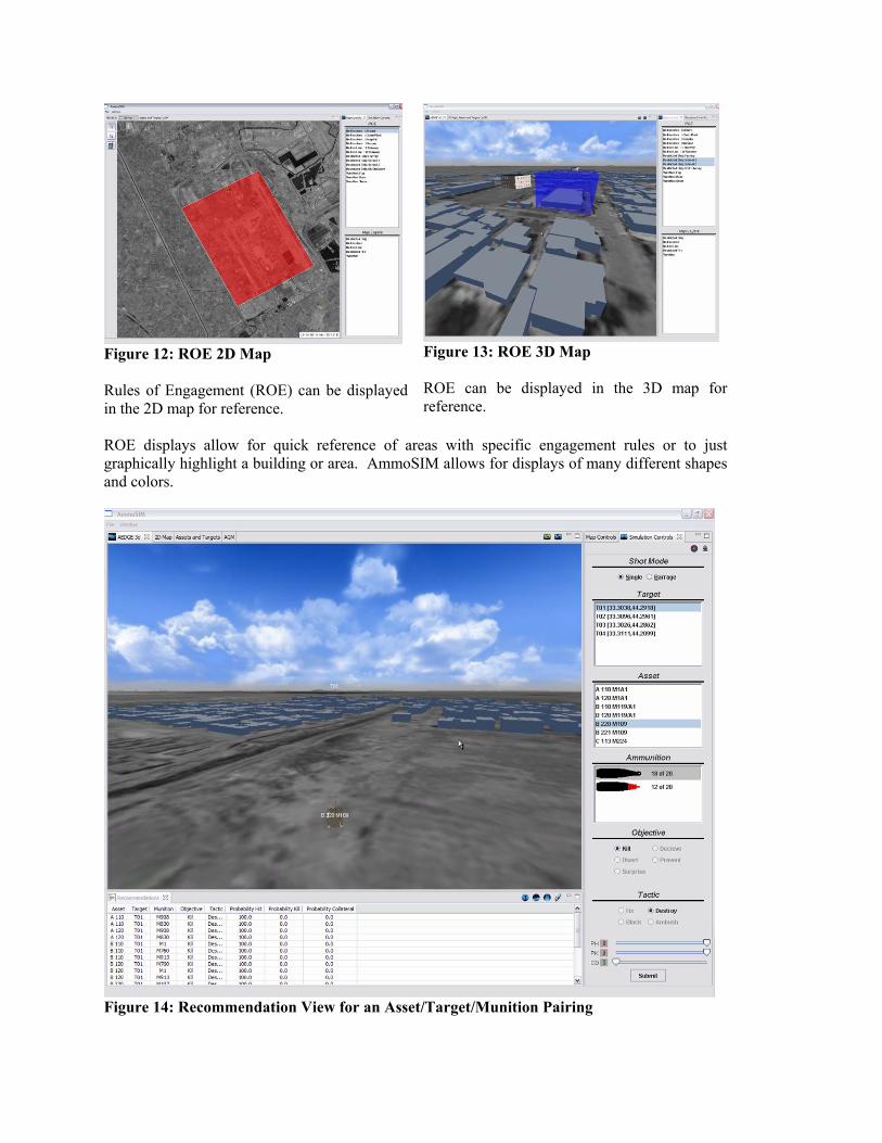
Figure 12: ROE 2D Map Rules of Engagement (ROE) can be displayed in the 2D map for reference.
Figure 13: ROE 3D Map ROE can be displayed in the 3D map for reference.
ROE displays allow for quick reference of areas with specific engagement rules or to just graphically highlight a building or area. AmmoSIM allows for displays of many different shapes and colors.
Figure 14: Recommendation View for an Asset/Target/Munition Pairing

Figure 15: Munition Trajectory Display of trajectories is displayed as a colored area surrounding the expected travel of the projectile to represent the circular error probable (CEP) of the projectile.
6. Summary and Conclusions 6.1. AmmoSIM integrates multiple data sources and a variety of separate data processing programs into one package. AmmoSIM connects to a number of data sources (DTSS, NGA, DTED, Worldwide construction database, etc.). Additional sources investigated were the Joint Weaponeering System (JWS) and NATO Armaments Ballistic Kernel (NABK). External toolkits were examined such as the Blast Effects Estimation Model (BEEM) and Structural Weapons Effects (SWE) API. The information gathered from this investigation proved useful in making AmmoSIM easily adaptable to new information sources.
6.2. AmmoSIM uses established methods mathematical principles. AmmoSIM utilizes a statistical model method as opposed to the standard Monte-Carlo methodology in calculating the most likely trajectory and error for a ballistic munition. AmmoSIM visually displays the trajectory and CEP in a 3D environment allowing the warfighter to instantly see the effects of a particular weapon and what may be inadvertently hit. The data is built from attack guidance matrix guidelines. AmmoSIM calculates the probabilities of hit, kill, and collateral damage instantly from the statistical model built into the software.

6.3. AmmoSIM displays the battlespace as an integrated picture showing recommendations directly to the user. AmmoSIM synchronizes the actions of C2 planners and in the field warfighters using a common display interchange. A 3D game engine is used to show the battlespace, and a 2D map to show relational data. The attack guidance matrix, target database, and asset database are used to construct the relevant information about the battlespace. Geo-specific building models are displayed directly inside the 3D game engine providing a realistic view of the battlespace. The rubble model, once fully implemented will provide a new tool to the soldier. Two models have been successfully developed to characterize the rubble pile created by the collapse of building. In both models, we assumed complete rubblization of the building and developed a rubble profile model using the size and composition of the collapsed structure to predict the rubble volume. These profile models include the size of footprint area surrounding the original building as well as the height of rubble pile at its center and along its periphery. The dimensions of the rubble pile have been adjusted to include the effects of buildings adjacent to the original collapsed building. At this stage of this effort, empirical data is needed to verify the predictive capabilities of the various models and processes developed. 6.4. Conclusion AmmoSIM is an intelligent agent-based urban tactical decision aid used by platoon, company, and battalion commanders to simulate and validate targeting effects during combat operations in urban terrain. In a near real-time simulated environment AmmoSIM simulates the direct employment and secondary effects of tanks, howitzers, and mortars against a given target(s) and the target area. It depicts the trajectory of these weapons in a 2D/3D view. AmmoSIM calculates the ballistic trajectory of given munitions and models the effects on the target in the surrounding area as it uses accessed data from planned terrain and tactical battlefield command and control sources. Commanders must increasingly plan MOUT actions in an environment where there is miniscule, if any, room for error. AmmoSIM provides recommended courses of action that enhance currently fielded situational awareness systems for planners and decision makers. AmmoSIM is a real-time, small footprint software package designed to run on laptop computers or better.
This paper shows the development and underlying mathematical structure behind AmmoSIM. In particular, the use of statistical analysis of the hit, kill, and collateral damage probabilities enhances greatly the ability of a soldier to determine the best weapon to use against a target. The rubble model development is also unique in showing the dimensions of the rubble produced for a given building and the quantity of explosive needed to produce rubblization. Finally, the visualization is an entirely new concept for ballistic targeting, and one that is receiving much attention. The capabilities that AmmoSIM brings to the war fighter are needed and will greatly enhance the lethality of our troops.

References [A04] D. Andersen, “AmmoSIM SBIR Phase I Final Technical Report,” SBIR Phase I Final Technical
Report to USACE TEC, 2004. [A99] Alisjahbana, S.W. “Dynamic Response of Large Space Building Floors to Dynamic Moving
Loads,” 3rd Asia-Pacific Conference on Shock and Impact Loads on Structures, T. Lok, and C. Lim, eds., Singapore, pp. 33-42, 1999.
[BN05] H Burleson and W. Noll, “AmmoSIM SBIR Phase I Option Final Report,” SBIR Phase I Option Final Technical Report to USACE TEC, 2005.
[NWB06] W Noll, R. Woodley, and J. Barker, “AmmoSIM SBIR Phase II Final Report,” SBIR Phase II Final Technical Report to USACE TEC, 2006.
[CZC01] M. Chen, Q. Zhu, and Z. Chen, “An Integrated Interactive Environment for Knowledge Discovery from Heterogeneous Data Resources,” Journal of Information & Software Technology, Vol. 43, pp. 487-496, 2001.
[ECD00] L. R. Elliott, S. Chaiken, M. Dalrymple, P. V. Petrov, & A. D. Stoyen. “Simulation-based Agent Support in a Synthetic Team-based C2 Task Environment,” Accepted for Proceedings of the 2000 Command and Control Research and Technology Symposium, June 26-29 2000.
[M795] http://www.globalsecurity.org/military/systems/munitions/m795.htm. [NKNW96] J. Neter, M.Kutner, C. Nachtsheim, and W. Wasserman, Applied Linear Regression Models,
3rd edition. McGraw-Hill Companies, Inc. 1996. [PKAD04] Physical model Knowledge Acquisition Document (PKAD), “Delivery Accuracy for Indirect
Fire Weapons”; U.S. Army Materiel Systems Analysis Activity, Aberdeen Proving Ground, Maryland; November 24, 2004; Distribution Limited to Department of Defense and DoD Contractors Only, Critical Technology, April 2000.
[YB96] Yarimer, E., and Brown, C.D.; “The Effect of Rubble Accumulation on the Mechanics of Demolition by Rapid Collapse,” UStructures Under Shock and Impact IVU; N. Jones and C. Brebbia, eds, WIT Press, UK; 1996; pp. 25-33.