Actuarial Mathematics and Life-Table Statisticsevs/s470/BookChaps/Chp6.pdf · Actuarial Mathematics and Life-Table Statistics Eric V. Slud Mathematics Department University of Maryland,

Actuarial Mathematics

and Life-Table Statistics

Eric V. SludMathematics Department

University of Maryland, College Park

c©2006

Chapter 6

Commutation Functions,Reserves & Select Mortality

In this Chapter, we consider first the historically important topic of Commu-tation Functions for actuarial calculations, and indicate why they lose theircomputational usefulness as soon as the insurer entertains the possibility (asdemographers often do) that life-table survival probabilities display someslow secular trend with respect to year of birth. We continue our treatmentof premiums and insurance contract valuation by treating briefly the ideaof insurance reserves and policy cash values as the life-contingent analogueof mortgage amortization and refinancing. The Chapter concludes with abrief section on Select Mortality, showing how models for select-populationmortality can be used to calculate whether modified premium and deferraloptions are sufficient protections for insurers to insure such populations.

6.1 Idea of Commutation Functions

The Commutation Functions are a computational device to ensure that netsingle premiums for life annuities, endowments, and insurances from the samelife table and figured at the same interest rate, for lives of differing ages andfor policies of differing durations, can all be obtained from a single table look-up. Historically, this idea has been very important in saving calculationallabor when arriving at premium quotes. Even now, assuming that a govern-

149

150 CHAPTER 6. COMMUTATION & RESERVES

ing life table and interest rate are chosen provisionally, company employeeswithout quantitative training could calculate premiums in a spreadsheet for-mat with the aid of a life table.

To fix the idea, consider first the contract with the simplest net-single-premium formula, namely the pure n-year endowment. The expected presentvalue of $1 one year in the future if the policyholder aged x is alive at thattime is denoted in older books as nEx and is called the actuarial presentvalue of a life-contingent n-year future payment of 1:

A 1x:n⌉ = nEx = vn

npx

Even such a simple life-table and interest-related function would seem to re-quire a table in the two integer parameters x, n, but the following expressionimmediately shows that it can be recovered simply from a single tabulatedcolumn:

A 1x:n⌉ =

vn+x ln+x

vx lx=

Dx+n

Dx

, Dy ≡ vy ly (6.1)

In other words, at least for integer ages and durations we would simplyaugment the insurance-company life-table by the column Dx. The additionof just a few more columns allows the other main life-annuity and insurancequantities to be recovered with no more than simple arithmetic. Thus, if webegin by considering whole life insurances (with only one possible paymentat the end of the year of death), then the net single premium is re-written

Ax = A1x:∞⌉ =

∞∑

k=0

vk+1kpx · qx+k =

∞∑

k=0

vx+k+1 (lx+k − lx+k+1)

vx lx

=∞∑

y=x

vy+1 dy

Dx

=Mx

Dx

, Mx ≡∞∑

y=x

vy+1 dy

The insurance of finite duration also has a simple expression in terms of thesame commutation columns M, D :

A1x:n⌉ =

n−1∑

k=0

vk+1 dk+x

Dx

=Mx − Mx+n

Dx

(6.2)

6.1. IDEA OF COMMUTATION FUNCTIONS 151

Next let us pass to to life annuities. Again we begin with the life annuity-due of infinite duration:

ax = ax:∞⌉ =∞∑

k=0

vk+x lk+x

Dx

=Nx

Dx

, Nx =∞∑

y=x

vy ly (6.3)

The commutation column Nx turns is the reverse cumulative sum of theDx column:

Nx =∞∑

y=x

Dy

The expected present value for the finite-duration life-annuity due is obtainedas a simple difference

ax:n⌉ =n−1∑

k=0

vk+x lx+k

Dx

=Nx − Nx+n

Dx

There is no real need for a separate commutation column Mx since, aswe have seen, there is an identity relating net single premiums for whole lifeinsurances and annuities:

Ax = 1 − d ax

Writing this identity with Ax and ax replaced by their respective commutation-function formulas, and then multupliying through by Dx, immediately yields

Mx = Dx − dNx (6.4)

Based on these tabulated commutation columns D, M, N , a quan-titatively unskilled person could use simple formulas and tables to provideon-the-spot insurance premium quotes, a useful and desirable outcome evenin these days of accessible high-powered computing. Using the case-(i) inter-polation assumption, the m-payment-per-year net single premiums A(m)1

x:n⌉

and a(m)x:n⌉ would be related to their single-payment counterparts (whose

commutation-function formulas have just been provided) through the stan-dard formulas

A(m)1x:n⌉ =

i

i(m)A1

x:n⌉ , a(m)x:n⌉ = α(m) ax:n⌉ − β(m)

(

1 − A 1x:n⌉

)


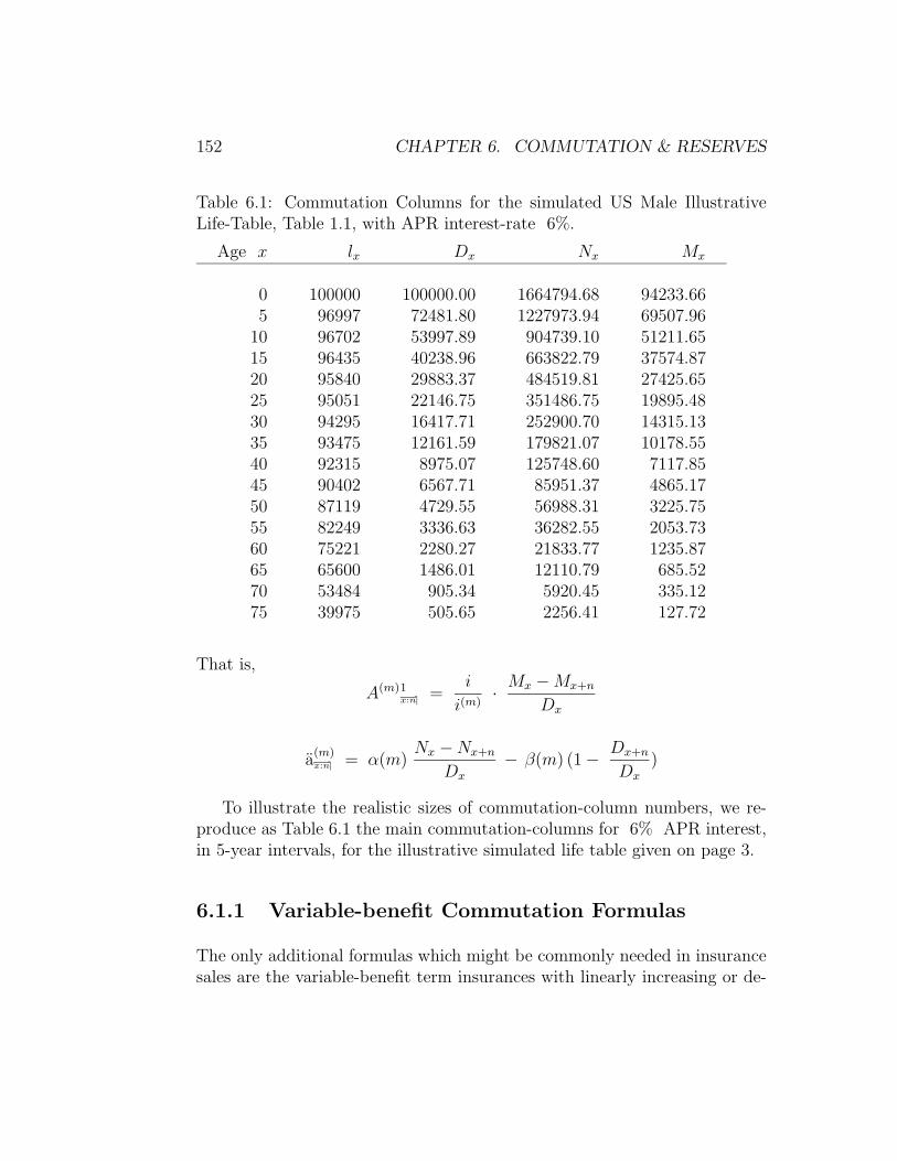
Table 6.1: Commutation Columns for the simulated US Male IllustrativeLife-Table, Table 1.1, with APR interest-rate 6%.

Age x lx Dx Nx Mx

0 100000 100000.00 1664794.68 94233.665 96997 72481.80 1227973.94 69507.96

10 96702 53997.89 904739.10 51211.6515 96435 40238.96 663822.79 37574.8720 95840 29883.37 484519.81 27425.6525 95051 22146.75 351486.75 19895.4830 94295 16417.71 252900.70 14315.1335 93475 12161.59 179821.07 10178.5540 92315 8975.07 125748.60 7117.8545 90402 6567.71 85951.37 4865.1750 87119 4729.55 56988.31 3225.7555 82249 3336.63 36282.55 2053.7360 75221 2280.27 21833.77 1235.8765 65600 1486.01 12110.79 685.5270 53484 905.34 5920.45 335.1275 39975 505.65 2256.41 127.72

That is,

A(m)1x:n⌉ =

i

i(m)·

Mx − Mx+n

Dx

a(m)x:n⌉ = α(m)

Nx − Nx+n

Dx

− β(m) (1 −Dx+n

Dx

)

To illustrate the realistic sizes of commutation-column numbers, we re-produce as Table 6.1 the main commutation-columns for 6% APR interest,in 5-year intervals, for the illustrative simulated life table given on page 3.

6.1.1 Variable-benefit Commutation Formulas

The only additional formulas which might be commonly needed in insurancesales are the variable-benefit term insurances with linearly increasing or de-

6.1. IDEA OF COMMUTATION FUNCTIONS 153

creasing benefits, and we content ourselves with showing how an additionalcommutation-column could serve here. First consider the infinite-durationpolicy with linearly increasing benefit

IAx =∞∑

k=0

(k + 1) vk+1kpx · qx+k

This net single premium can be written in terms of the commutation func-tions already given together with

Rx =∞∑

k=0

(x + k + 1) vx+k+1 dx+k

Clearly, the summation defining IAx can be written as

∞∑

k=0

(x + k + 1) vk+1kpx · qx+k − x

∞∑

k=0

vk+1kpx · qx+k =

Rx

Dx

− xMx

Dx

Then, as we have discussed earlier, the finite-duration linearly-increasing-benefit insurance has the expression

IA1x:n⌉ = IAx −

∞∑

k=n

(k + 1) vk+x+1 dx+k

Dx

=Rx − xMx

Dx

−Rx+n − xMx+n

Dx

and the net single premium for the linearly-decreasing-benefit insurance,which pays benefit n − k if death occurs between exact policy ages kand k + 1 for k = 0, . . . , n − 1, can be obtained from the increasing-benefit insurance through the identity

DA1x:n⌉ = (n + 1)A1

x:n⌉ − IA1x:n⌉

Throughout all of our discussions of premium calculation — not just thepresent consideration of formulas in terms of commutation functions — wehave assumed that for ages of prospective policyholders, the same interestrate and life table would apply. In a future Chapter, we shall consider theproblem of premium calculation and reserving under variable and stochasticinterest-rate assumptions, but for the present we continue to fix the interestrate i. Here we consider briefly what would happen to premium calcula-tion and the commutation formalism if the key assumption that the same


life table applies to all insureds were to be replaced by an assumption in-volving interpolation between (the death rates defined by) two separate lifetables applying to different birth cohorts. This is a particular case of atopic which we shall also take up in a future chapter, namely how extra(‘covariate’ ) information about a prospective policyholder might change thesurvival probabilities which should be used to calculate premiums for thatpolicyholder.

6.1.2 Secular Trends in Mortality

Demographers recognize that there are secular shifts over time in life-tableage-specific death-rates. The reasons for this are primarily related to publichealth (e.g., through the eradication or successful treatment of certain dis-ease conditions), sanitation, diet, regulation of hours and conditions of work,etc. As we have discussed previously in introducing the concept of force ofmortality, the modelling of shifts in mortality patterns with respect to likelycauses of death at different ages suggests that it is most natural to expressshifts in mortality in terms of force-of-mortality and death rates rather thanin terms of probability density or population-wide relative numbers of deathsin various age-intervals. One of the simplest models of this type, used forprojections over limited periods of time by demographers (cf. the text Intro-duction to Demography by M. Spiegelman), is to view age-specific death-ratesqx as locally linear functions of calendar time t. Mathematically, it may beslightly more natural to make this assumption of linearity directly about theforce of mortality. Suppose therefore that in calendar year t, the force ofmortality µ

(t)x at all ages x is assumed to have the form

µ(t)x = µ(0)

x + bx t (6.5)

where µ(0)x is the force-of-mortality associated with some standard life table

as of some arbitrary but fixed calendar-time origin t = 0. The age-dependentslope bx will generally be extremely small. Then, placing superscripts (t)

over all life-table entries and ratios to designate calendar time, we calculate

kp(t)x = exp

(

−

∫ k

0

µ(t)x+u du

)

= kp(t)x · exp(−t

k−1∑

j=0

bx+j)

6.2. RESERVE & CASH VALUE OF A SINGLE POLICY 155

If we denote

Bx =x∑

y=0

by

and assume that the life-table radix l0 is not taken to vary with calendartime, then the commutation-function Dx = D

(t)x takes the form

D(t)x = vx l0 xp

(t)0 = D(0)

x e−tBx (6.6)

Thus the commutation-columns D(0)x (from the standard life-table) and Bx

are enough to reproduce the time-dependent commutation column D, butnow the calculation is not quite so simple, and the time-dependent commu-tation columns M, N become

M (t)x =

∞∑

y=x

vy (l(t)y − l(t)y+1) =

∞∑

y=x

D(0)y e−tBy

(

1 − e−t by+1 q(0)y

)

(6.7)

N (t)x =

∞∑

y=x

D(0)y e−tBy (6.8)

For simplicity, one might replace equation (6.7) by the approximation

M (t)x =

∞∑

y=x

D(0)y

(

p(0)y + t by+1 q(0)

y

)

e−tBy

None of these formulas would be too difficult to calculate with, for exampleon a hand-calculator; moreover, since the calendar year t would be fixed forthe printed tables which an insurance salesperson would carry around, thevirtues of commutation functions in providing quick premium-quotes wouldnot be lost if the life tables used were to vary systematically from one calendaryear to the next.

6.2 Reserve & Cash Value of a Single Policy

In long-term insurance policies paid for by level premiums, it is clear thatsince risks of death rise very rapidly with age beyond middle-age, the earlypremium payments must to some extent exceed the early insurance costs.


Our calculation of risk premiums ensures by definition that for each insuranceand/or endowment policy, the expected total present value of premiums paidin will equal the expected present value of claims to be paid out. However,it is generally not true within each year of the policy that the expectedpresent value of amounts paid in are equal to the expected present value ofamounts paid out. In the early policy years, the difference paid in versusout is generally in the insurer’s favor, and the surplus must be set aside as areserve against expected claims in later policy-years. It is the purpose of thepresent section to make all of these assertions mathematically precise, and toshow how the reserve amounts are to be calculated. Note once and for all thatloading plays no role in the calculation of reserves: throughout this Section,‘premiums’ refer only to pure-risk premiums. The loading portion of actualpremium payments is considered either as reimbursement of administrativecosts or as profit of the insurer, but in any case does not represent buildupof value for the insured.

Suppose that a policyholder aged x purchased an endowment or insur-ance (of duration at least t) t years ago, paid for with level premiums, andhas survived to the present. Define the net (level) premium reserve asof time t to be the excess tV of the expected present value of the amountto be paid out under the contract in future years over the expected presentvalue of further pure risk premiums to be paid in (including the premiumpaid immediately, in case policy age t coincides with a time of premium-payment). Just as the notations P 1

x:n⌉, P 1x:n⌉, etc., are respectively used to

denote the level annual premium amounts for a term insurance, an endow-ment, etc., we use the same system of sub- and superscripts with the symbol

tV to describe the reserves on these different types of policies.

By definition, the net premium reserve of any of the possible types ofcontract as of policy-age t = 0 is 0 : this simply expresses the balancebetween expected present value of amounts to be paid into and out of theinsurer under the policy. On the other hand, the terminal reserve under thepolicy, which is to say the reserve nV just before termination, will differfrom one type of policy to another. The main possibilities are the pure terminsurance, with reserves denoted tV

1x:n⌉ and terminal reserve nV

1x:n⌉ = 0, and

the endowment insurance, with reserves denoted tV1

x:n⌉ and terminal reserve

nV1

x:n⌉ = 1. In each of these two examples, just before policy terminationthere are no further premiums to be received or insurance benefits to be paid,


so that the terminal reserve coincides with the terminal (i.e., endowment)benefit to be paid at policy termination. Note that for simplicity, we donot consider here the insurances or endowment insurances with m > 1possible payments per year. The reserves for such policies can be obtainedas previously discussed from the one-payment-per-year case via interpolationformulas.

The definition of net premium reserves is by nature prospective, referringto future payment streams and their expected present values. From the def-inition, the formulas for reserves under the term and endowment insurancesare respectively given by:

tV1

x:n⌉ = A1x+t:n−t⌉ − P 1

x:n⌉ · ax+t:n−t⌉ (6.9)

tVx:n⌉ = Ax+t:n−t⌉ − Px:n⌉ · ax+t:n−t⌉ (6.10)

One identity from our previous discussions of net single premiums im-mediately simplifies the description of reserves for endowment insurances.Recall the identity

ax:n⌉ =1 − Ax:n⌉

d=⇒ Ax:n⌉ = 1 − d ax:n⌉

Dividing the second form of this identity through by the net single premiumfor the life annuity-due, we obtain

Px:n⌉ =1

ax:n⌉

− d (6.11)

after which we immediately derive from the definition the reserve-identity

tVx:n⌉ = ax+t:n−t⌉

(

Px+t:n−t⌉ − Px:n⌉

)

= 1 −ax+t:n−t⌉

ax:n⌉

(6.12)

6.2.1 Retrospective Formulas & Identities

The notion of reserve discussed so far expresses a difference between expectedpresent value of amounts to be paid out and to be paid in to the insurer datingfrom t years following policy initiation, conditionally given the survival ofthe insured life aged x for the additional t years to reach age x + t. It


stands to reason that, assuming this reserve amount to be positive, theremust have been up to time t an excess of premiums collected over insuranceacquired up to duration t. This latter amount is called the cash value ofthe policy when accumulated actuarially to time t, and represents a cashamount to which the policyholder is entitled (less administrative expenses)if he wishes to discontinue the insurance. (Of course, since the insured haslived to age x + t, in one sense the insurance has not been ‘used’ at allbecause it did not generate a claim, but an insurance up to policy age t wasin any case the only part of the purchased benefit which could have broughta payment from the insurer up to policy age t.) The insurance boughthad the time-0 present value A1

x:t⌉, and the premiums paid prior to time t

had time-0 present value ax:t⌉ · P , where P denotes the level annualizedpremium for the duration-n contract actually purchased.

To understand clearly why there is a close connection between retrospec-tive and prospective differences between expected (present value of) amountspaid in and paid out under an insurance/endowment contract, we state ageneral and slightly abstract proposition.

Suppose that a life-contingent payment stream (of duration n atleast t) can be described in two stages, as conferring a benefit ofexpected time-0 present value Ut on the policy-age-interval [0, t)(up to but not including policy age t ), and also conferring abenefit if the policyholder is alive as of policy age t with expectedpresent value as of time t which is equal to Ft. Then thetotal expected time-0 present value of the contractualpayment stream is

Ut + vttpx Ft

Before applying this idea to the balancing of prospective and retrospective re-serves, we obtain without further effort three useful identities by recognizingthat a term life-insurance, insurance endowment, and life annuity-due (all ofduration n) can each be divided into a before- and after- t component alongthe lines of the displayed Proposition. (Assume for the following discussionthat the intermediate duration t is also an integer.) For the insurance, thebenefit Ut up to t is A1

x:t⌉, and the contingent after-t benefit Ft is

A1x+t:n−t⌉

. For the endowment insurance, Ut = A1x:t⌉

and Ft = Ax+t:n−t⌉.


Finally, for the life annuity-due, Ut = ax:t⌉ and Ft = ax+t:n−t⌉. Assemblingthese facts using the displayed Proposition, we have our three identities:

A1x:n⌉ = A1

x:t⌉ + vttpx A1

x+t:n−t⌉ (6.13)

Ax:n⌉ = A1x:t⌉ + vt

tpx Ax+t:n−t⌉ (6.14)

ax:n⌉ = ax:t⌉ + vttpx ax+t:n−t⌉ (6.15)

The factor vttpx, which discounts present values from time t to the

present values at time 0 contingent on survival to t, has been called abovethe actuarial present value. It coincides with tEx = A 1

x:t⌉, the expected

present value at 0 of a payment of 1 to be made at time t if the life aged xsurvives to age x+t. This is the factor which connects the excess of insuranceover premiums on [0, t) with the reserves tV on the insurance/endowmentcontracts which refer prospectively to the period [t, n]. Indeed, substitutingthe identities (6.13), (6.14), and (6.15) into the identities

A1x:n⌉ = P 1

x:n⌉ ax:n⌉ , Ax:n⌉ = Px:n⌉ ax:n⌉

yields

vttpx tV

1x:n⌉ = −

[

A1x:t⌉ − P 1

x:n⌉ ax:n⌉

]

(6.16)

vttpx tVx:n⌉ = −

[

Ax:t⌉ − Px:t⌉ ax:n⌉

]

(6.17)

The interpretation in words of these last two equations is that the actuarialpresent value of the net (level) premium reserve at time t (of either theterm insurance or endowment insurance contract) is equal to the negative ofthe expected present value of the difference between the contract proceedsand the premiums paid on [0, t).

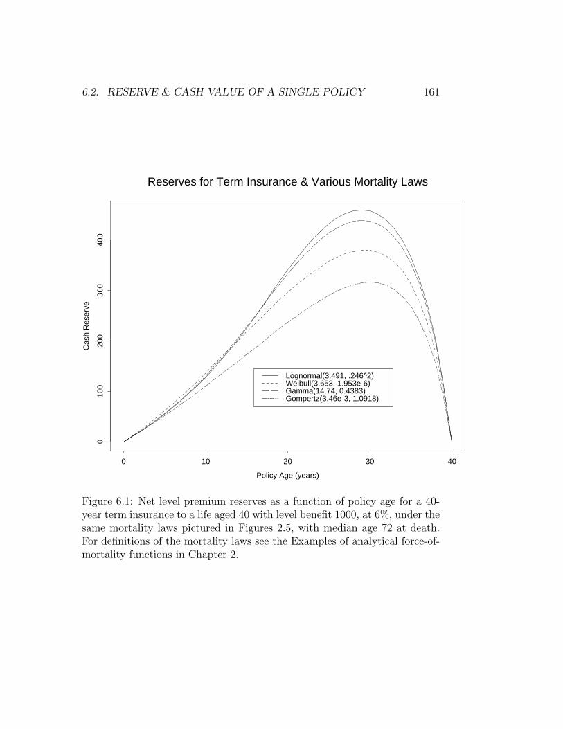
Figure 6.1 provides next an illustrative set of calculated net level premiumreserves, based upon 6% interest, for a 40-year term life insurance with face-amount 1, 000 for a life aged 40. The mortality laws used in this calculation,chosen from the same families of laws used to illustrate force-of-mortalitycurves in Figures 2.3 and 2.4 in Chapter 2, are the same plausible mortalitylaws whose survival functions are pictured in Figure 2.5. These mortalitylaws are realistic in the sense that they closely mirror the US male mortalityin 1959 (cf. plotted points in Figure 2.5.) The cash-reserve curves tV40:40⌉

as functions of t = 0, . . . , 40 are pictured graphically in Figure 6.1. Note


that these reserves can be very substantial: at policy age 30, the reserveson the $1000 term insurance are respectively $459.17, $379.79, $439.06, and$316.43.

6.2.2 Relating Insurance & Endowment Reserves

The simplest formulas for net level premium reserves in a general contractarise in the case of endowment insurance tV

1x:n⌉, as we have seen in formula

(6.12). In fact, for endowment and/or insurance contracts in which the periodof payment of level premiums coincides with the (finite or infinite) policyduration, the reserves for term-insurance and pure-endowment can also beexpressed rather simply in terms of tVx:n⌉. Indeed, reasoning from firstprinciples with the prospective formula, we find for the pure endowment

tV1

x:n⌉ = vn−tn−tpx+t −

vnnpx

ax:n⌉

ax+t:n−t⌉

from which, by substitution of formula (6.12), we obtain

V 1x:n⌉ = vn−t

n−tpx+t − vnnpx

(

1 − tVx:n⌉

)

(6.18)

Then, for net level reserves or cash value on a term insurance, we conclude

V1x:n⌉ = (1 − vn

npx) tVx:n⌉ + vnnpx − vn−t

n−tpx+t (6.19)

6.2.3 Reserves under Constant Force of Mortality

We have indicated above that the phenomenon of positive reserves relates insome way to the aging of human populations, as reflected in the increasingforce of mortality associated with life-table survival probabilities. A simplebenchmark example helps us here: we show that when life-table survival isgoverned at all ages x and greater by a constant force of mortality µ,the reserves for term insurances are identically 0. In other words, theexpected present value of premiums paid in within each policy year exactlycompensates, under constant force of mortality, for the expected presentvalue of the amount to be paid out for that same policy year.


Reserves for Term Insurance & Various Mortality Laws

Policy Age (years)

Cas

h R

eser

ve

0 10 20 30 40

010

020

030

040

0

Lognormal(3.491, .246^2)Weibull(3.653, 1.953e-6)Gamma(14.74, 0.4383)Gompertz(3.46e-3, 1.0918)

Figure 6.1: Net level premium reserves as a function of policy age for a 40-year term insurance to a life aged 40 with level benefit 1000, at 6%, under thesame mortality laws pictured in Figures 2.5, with median age 72 at death.For definitions of the mortality laws see the Examples of analytical force-of-mortality functions in Chapter 2.


The calculations here are very simple. Reasoning from first principles,under constant force of mortality

A1x:n⌉ =

n−1∑

k=0

vk+1 e−µ k (1 − e−µ) = (eµ − 1) (ve−µ)1 − (ve−µ)n

1 − ve−µ

while

ax:n⌉ =n−1∑

k=0

vk e−µ k =1 − (ve−µ)n

1 − ve−µ

It follows from these last two equations that

P 1x:n⌉ = v (1 − e−µ)

which does not depend upon either age x (within the age-range whereconstant force of mortality holds) or n . The immediate result is that for0 < t < n

tV1

x:n⌉ = ax+t:n−t⌉

(

P 1x+t:n−t⌉ − P 1

x:n⌉

)

= 0

By contrast, since the terminal reserve of an endowment insurance must be1 even under constant force of mortality, the intermediate net level premiumreserves for endowment insurance must be positive and growing. Indeed, wehave the formula deriving from equation (6.12)

tVx:n⌉ = 1 −ax+t:n−t⌉

ax:n⌉

= 1 −1 − (ve−µ)n−t

1 − (ve−µ)n

6.2.4 Reserves under Increasing Force of Mortality

Intuitively, we should expect that a force-of-mortality function which is ev-erywhere increasing for ages greater than or equal to x will result in inter-mediate reserves for term insurance which are positive at times between 0, nand in reserves for endowment insurance which increase from 0 at t = 0 to1 at t = n. In this subsection, we prove those assertions, using the simpleobservation that when µ(x + y) is an increasing function of positive y,

kpx+y = exp(−

∫ k

0

µ(x + y + z) dz) ց in y (6.20)


First suppose that 0 ≤ s < t ≤ n, and calculate using the displayed factthat kpx+y decreases in y,

ax+t:n−t⌉ =n−t−1∑

k=0

vk+1kpx+t ≤

n−t−1∑

k=0

vk+1kpx+s < ax+s:n−s⌉

Therefore ax+t:n−t⌉ is a decreasing function of t, and by formula (6.12),

tVx:n⌉ is an increasing function of t, ranging from 0 at t = 0 to 1 att = 1.

It remains to show that for force of mortality which is increasing in age,the net level premium reserves tV

1x:n⌉ for term insurances are positive for

t = 1, . . . , n− 1. By equation (6.9) above, this assertion is equivalent to theclaim that

A1x+t:n−t⌉/ax+t:n−t⌉ > A1

x:n⌉/ax:n⌉

To see why this is true, it is instructive to remark that each of the displayedratios is in fact a multiple v times a weighted average of death-rates: for0 ≤ s < n,

A1x+s:n−s⌉

ax+s:n−s⌉

= v{

∑n−s−1k=0 vk

kpx+s qx+s+k∑n−s−1

k=0 vkkpx+s

}

Now fix the age x arbitrarily, together with t ∈ {1, . . . , n− 1}, and define

q =

∑n−1j=t vj

jpx qx+j∑n−1

j=t vjjpx

Since µx+y is assumed increasing for all y, we have from formula (6.20)that qx+j = 1 − px+j is an increasing function of j, so that for k < t ≤j, qx+k < qx+j and

for all k ∈ {0, . . . , t − 1} , qx+k < q (6.21)

Moreover, dividing numerator and denominator of the ratio defining q byvt

tpx gives the alternative expression

v q =

∑n−t−1a=0 va

apx+t qx+t+a∑n−t−1

a=0 vaapx+t

= P 1x+t:n−t⌉


Finally, using equation (6.21) and the definition of q once more, we calculate

A1x:n⌉

ax:n⌉

= v(

∑t−1k=0 vk

kpx qx+k +∑n−t−1

j=t vjjpx qx+j

∑t−1k=0 vk

kpx +∑n−t−1

j=t vjjpx

)

= v(

∑t−1k=0 vk

kpx qx+k + q∑n−t−1

j=t vjjpx

∑t−1k=0 vk

kpx +∑n−t−1

j=t vjjpx

)

< v q = P 1x+t:n−t⌉

as was to be shown. The conclusion is that under the assumption of increasingforce of mortality for all ages x and larger, tV

1x:n⌉ > 0 for t = 1, . . . , n− 1.

6.2.5 Recursive Calculation of Reserves

The calculation of reserves can be made very simple and mechanical in nu-merical examples with small illustrative life tables, due to the identities (6.13)and (6.14) together with the easily proved recursive identities (for integerst)

A1x:t+1⌉ = A1

x:t⌉ + vt+1tpx qx+t

Ax:t+1⌉ = Ax:t⌉ − vttpx + vt+1

tpx = Ax:t⌉ − d vttpx

ax:t+1⌉ = ax:t⌉ + vttpx

Combining the first and third of these recursions with (6.13), we find

tV1

x:n⌉ =−1

vttpx

(

A1x:t⌉ − P 1

x:n⌉ ax:t⌉

)

=−1

vttpx

(

A1x:t+1⌉ − vt+1

tpx qx+t − P 1x:n⌉

[

ax:t+1⌉ − vttpx

] )

= v px+t t+1V1

x:n⌉ + v qx+t − P 1x:n⌉

The result for term-insurance reserves is the single recursion

tV1

x:n⌉ = v px+t t+1V1

x:n⌉ + v qx+t − P 1x:n⌉ (6.22)

which we can interpret in words as follows. The reserves at integer policy-age t are equal to the sum of the one-year-ahead actuarial present valueof the reserves at time t + 1 and the excess of the present value of this


year’s expected insurance payout (v qx+t) over this year’s received premium(P 1

x:n⌉).

A completely similar algebraic proof, combining the one-year recursionsabove for endowment insurance and life annuity-due with identity (6.14),yields a recursive formula for endowment-insurance reserves (when t < n) :

tVx:n⌉ = v px+t t+1Vx:n⌉ + v qx+t − P 1x:n⌉ (6.23)

The verbal intepretation is as before: the future reserve is discounted by theone-year actuarial present value and added to the expected present value ofthe one-year term insurance minus the one-year cash (risk) premium.

6.2.6 Paid-Up Insurance

An insured may want to be aware of the cash value (equal to the reserve)of an insurance or endowment either in order to discontinue the contractand receive the cash or to continue the contract in its current form andborrow with the reserve as collateral. However, it may also happen for variousreasons that an insured may want to continue insurance coverage but isno longer able or willing to par further premiums. In that case, for anadministrative fee the insurer can convert the premium reserve to a singlepremium for a new insurance (either with the same term, or whole-life) withlesser benefit amount. This is really not a new topic, but a combination of theprevious formulas for reserves and net single premiums. In this sub-section,we give the simplified formula for the case where the cash reserve is used as asingle premium to purchase a new whole-life policy. Two illustrative workedexamples on this topic are given in Section 6.6 below.

The general formula for reserves, now specialized for whole-life insur-ances, is

tVx = Ax+t −Ax

ax

· ax+t = 1 −ax+t

ax

This formula, which applies to a unit face amount, would be multipliedthrough by the level benefit amount B. Note that loading is disregardedin this calculation. The idea is that any loading which may have appliedhas been collected as part of the level premiums; but in practice, the insurermight apply some further (possibly lesser) loading to cover future adminis-trative costs. Now if the cash or reserve value tVx is to serve as net single


premium for a new insurance, the new face-amount F is determined as ofthe t policy-anniversary by the balance equation

B · tVx = F · Ax+t

which implies that the equivalent face amount of paid-up insurance asof policy-age t is

F =B tVx

Ax+t

= B

(

1 −ax+t

ax

)

/

(1 − d ax+t) (6.24)

6.3 Select Mortality Tables & Insurance

Insurers are often asked to provide life insurance converage to groups and/orindividuals who belong to special populations with mortality significantlyworse than that of the general population. Yet such select populationsmay not be large enough, or have a sufficiently long data-history, within theinsurer’s portfolio for survival probabilities to be well-estimated in-house. Insuch cases, insurers may provide coverage under special premiums and terms.The most usual example is that such select risks may be issued insurance withrestricted or no benefits for a specified period of time, e.g. 5 years. The statedrationale is that after such a period of deferral, the select group’s mortalitywill be sufficiently like the mortality of the general population in order thatthe insurer will be adequately protected if the premium in increased by somestandard multiple. In this Section, a slightly artifical calculation along theselines illustrates the principle and gives some numerical examples.

Assume for simplicity that the general population has constant force ofmortality µ, and that the select group has larger force of mortality µ∗. Ifthe interest rate is i, and v = 1/(1+ i), then the level yearly risk premiumfor a k-year deferred whole-life insurance (of unit amount, payable at the endof the year of death) to a randomly selected life (of any specified age x) fromthe general population is easily calculated to be

Level Risk Premium = vkkpx Ax+k/ax = (1 − e−µ) vk+1 e−µk (6.25)

If this premium is multiplied by a factor κ > 1 and applied as the riskpremium for a k-year deferred whole-life policy to a member of the select

6.3. SELECT MORTALITY TABLES & INSURANCE 167

Table 6.2: Excess payout as given by formula (6.26) under a k-year deferredwhole life insurance with benefit $1000, issued to a select population withconstant force of mortality µ∗ for a level yearly premium which is a multipleκ times the pure risk premium for the standard population which has force-of-mortality µ. Interest rate is i = 0.06 APR throughout.

k µ µ∗ κ Excess Payout

0 0.02 0.03 1 1090 0.02 0.03 2 -1125 0.02 0.03 1 635 0.02 0.03 1.42 00 0.05 0.10 1 2990 0.05 0.10 3 -3305 0.05 0.10 1 955 0.05 0.10 1.52 03 0.05 0.10 1 953 0.05 0.10 1.68 0

population, then the expected excess (per unit of benefit) of the amountpaid out under this select policy over the risk premiums collected, is

Excess Payout = vkkp

∗

x A∗

x+k − κ (1 − e−µ) vk+1 e−µk a∗x

=vk+1

1 − ve−mu∗

{

(1 − e−µ)e−µk − (1 − e−µ∗

)e−µ∗k}

(6.26)

where the probability, insurance, and annuity notations with superscripts ∗

are calculated using the select mortality distribution with force of mortalityµ∗. Because of the constancy of forces of mortality both in the general andthe select populations, the premiums and excess payouts do not depend onthe age of the insured. Table 6.3 shows the values of some of these excesspayouts, for i = 0.06, under several combinations of k, µ, µ∗, and κ. Notethat in these examples, select mortality with force of mortality multiplied by1.5 or 2 is offset, with sufficient protection to the insurer, by an increase of40–60% in premium on whole-life policies deferring benefits by 3 or 5 years.

Additional material will be added to this Section later. A calculation


along the same lines as the foregoing Table, but using the Gompertz(3.46e −3, 1.0918) mortality law previously found to approximate well the realisticLife Table data in Table 1.1, will be included for completeness.

6.4 Exercise Set 6

For the first problem, use the Simulated Illustrative Life Table with commu-tator columns given as Table 6.1 on page 152, using 6% APR as the goingrate of interest. (Also assume, wherever necessary, that the distribution ofdeaths within whole years of age is uniform.)

(1). (a) Find the level premium for a 20-year term insurance of $5000 foran individual aged 45, which pays at the end of the half-year of death, wherethe payments are to be made semi-annually.

(b) Find the level annual premium for a whole-life insurance for anindividual aged 35, which pays $30,000 at the end of year of death if deathoccurs before exact age 55 and pays $60,000 at the instant (i.e., day) of deathat any later age.

(2). You are given the following information, indirectly relating to the fixedrate of interest i and life-table survival probabilities kpx .

(i) For a one-payment-per-year level-premium 30-year endowment insur-ance of 1 on a life aged x, the amount of reduced paid-up endowmentinsurance at the end of 10 years is 0.5.

(ii) For a one-payment-per-year level-premium 20-year endowment in-surance of 1 on a life aged x+10, the amount of reduced paid-up insuranceat the end of 5 years is 0.3.

Assuming that cash values are equal to net level premium reserves andreduced paid-up insurances are calculated using the equivalence principle, sothat the cash value is equated to the net single premium of an endowmentinsurance with reduced face value, calculate the amount of reduced paid-upinsuranceat the end of 15 years for the 30-year endowment insuranceof 1on a life aged x. See the following Worked Examples for some relevantformulas.

6.4. EXERCISE SET 6 169

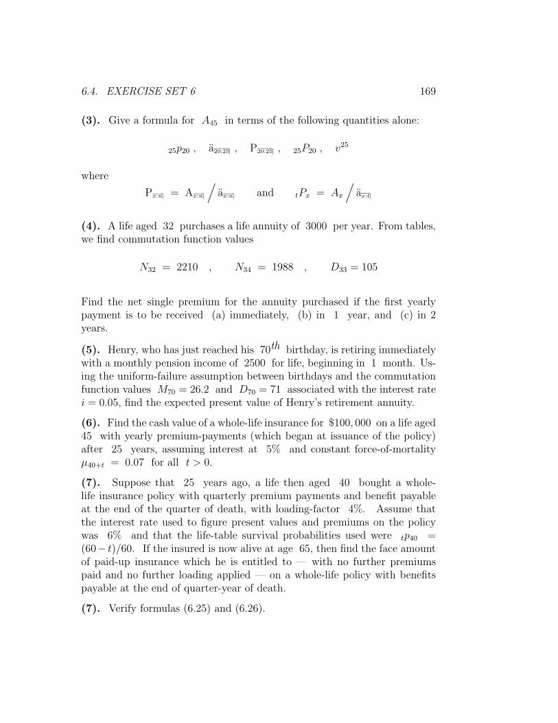
(3). Give a formula for A45 in terms of the following quantities alone:

25p20 , a20:25⌉ , P20:25⌉ , 25P20 , v25

where

Px:n⌉ = Ax:n⌉

/

ax:n⌉ and tPx = Ax

/

ax:t⌉

(4). A life aged 32 purchases a life annuity of 3000 per year. From tables,we find commutation function values

N32 = 2210 , N34 = 1988 , D33 = 105

Find the net single premium for the annuity purchased if the first yearlypayment is to be received (a) immediately, (b) in 1 year, and (c) in 2years.

(5). Henry, who has just reached his 70th birthday, is retiring immediatelywith a monthly pension income of 2500 for life, beginning in 1 month. Us-ing the uniform-failure assumption between birthdays and the commutationfunction values M70 = 26.2 and D70 = 71 associated with the interest ratei = 0.05, find the expected present value of Henry’s retirement annuity.

(6). Find the cash value of a whole-life insurance for $100, 000 on a life aged45 with yearly premium-payments (which began at issuance of the policy)after 25 years, assuming interest at 5% and constant force-of-mortalityµ40+t = 0.07 for all t > 0.

(7). Suppose that 25 years ago, a life then aged 40 bought a whole-life insurance policy with quarterly premium payments and benefit payableat the end of the quarter of death, with loading-factor 4%. Assume thatthe interest rate used to figure present values and premiums on the policywas 6% and that the life-table survival probabilities used were tp40 =(60− t)/60. If the insured is now alive at age 65, then find the face amountof paid-up insurance which he is entitled to — with no further premiumspaid and no further loading applied — on a whole-life policy with benefitspayable at the end of quarter-year of death.

(7). Verify formulas (6.25) and (6.26).


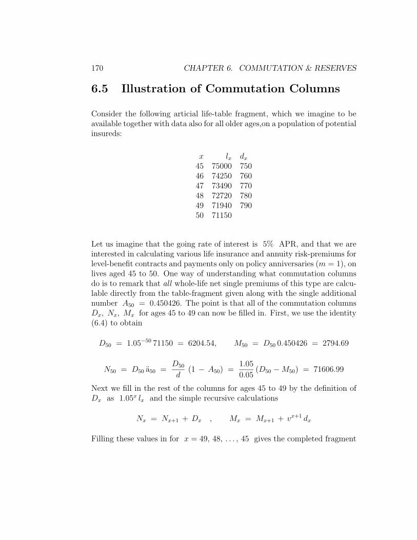
6.5 Illustration of Commutation Columns

Consider the following articial life-table fragment, which we imagine to beavailable together with data also for all older ages,on a population of potentialinsureds:

x lx dx

45 75000 75046 74250 76047 73490 77048 72720 78049 71940 79050 71150

Let us imagine that the going rate of interest is 5% APR, and that we areinterested in calculating various life insurance and annuity risk-premiums forlevel-benefit contracts and payments only on policy anniversaries (m = 1), onlives aged 45 to 50. One way of understanding what commutation columnsdo is to remark that all whole-life net single premiums of this type are calcu-lable directly from the table-fragment given along with the single additionalnumber A50 = 0.450426. The point is that all of the commutation columnsDx, Nx, Mx for ages 45 to 49 can now be filled in. First, we use the identity(6.4) to obtain

D50 = 1.05−50 71150 = 6204.54, M50 = D50 0.450426 = 2794.69

N50 = D50 a50 =D50

d(1 − A50) =

1.05

0.05(D50 − M50) = 71606.99

Next we fill in the rest of the columns for ages 45 to 49 by the definition ofDx as 1.05x lx and the simple recursive calculations

Nx = Nx+1 + Dx , Mx = Mx+1 + vx+1 dx

Filling these values in for x = 49, 48, . . . , 45 gives the completed fragment

6.6. EXAMPLES ON PAID-UP INSURANCE 171

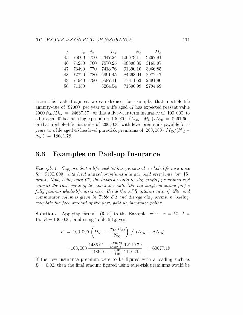
x lx dx Dx Nx Mx

45 75000 750 8347.24 106679.11 3267.8146 74250 760 7870.25 98808.85 3165.0747 73490 770 7418.76 91390.10 3066.8548 72720 780 6991.45 84398.64 2972.4749 71940 790 6587.11 77811.53 2891.8050 71150 6204.54 71606.99 2794.69

From this table fragment we can deduce, for example, that a whole-lifeannuity-due of $2000 per year to a life aged 47 has expected present value2000N47/D47 = 24637.57 , or that a five-year term insurance of 100, 000 toa life aged 45 has net single premium 100000 · (M45−M50)/D50 = 5661.66 ,or that a whole-life insurance of 200, 000 with level premiums payable for 5years to a life aged 45 has level pure-risk premiums of 200, 000 · M45/(N45−N50) = 18631.78.

6.6 Examples on Paid-up Insurance

Example 1. Suppose that a life aged 50 has purchased a whole life insurancefor $100, 000 with level annual premiums and has paid premiums for 15years. Now, being aged 65, the insured wants to stop paying premiums andconvert the cash value of the insurance into (the net single premium for) afully paid-up whole-life insurance. Using the APR interest rate of 6% andcommutator columns given in Table 6.1 and disregarding premium loading,calculate the face amount of the new, paid-up insurance policy.

Solution. Applying formula (6.24) to the Example, with x = 50, t =15, B = 100, 000, and using Table 6.1,gives

F = 100, 000

(

D65 −N65 D50

N50

)

/

(D65 − dN65)

= 100, 0001486.01 − 4729.55

56988.3112110.79

1486.01 − 0.061.06

12110.79= 60077.48

If the new insurance premium were to be figured with a loading such asL′ = 0.02, then the final amount figured using pure-risk premiums would be


divided by 1.02, because the cash value would then be regarded as a singlerisk premium which when inflated by the factor 1+L′ purchases the contractof expected present value F · Ax+t.

The same ideas can be applied to the re-figuring of the amount of otherinsurance contracts, such as an endowment, based upon an incomplete streamof premium payments.

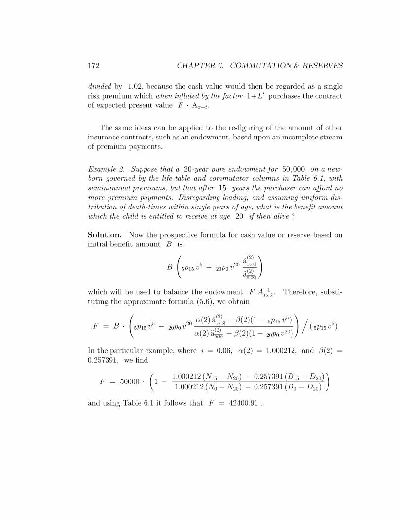
Example 2. Suppose that a 20-year pure endowment for 50, 000 on a new-born governed by the life-table and commutator columns in Table 6.1, withseminannual premiums, but that after 15 years the purchaser can afford nomore premium payments. Disregarding loading, and assuming uniform dis-tribution of death-times within single years of age, what is the benefit amountwhich the child is entitled to receive at age 20 if then alive ?

Solution. Now the prospective formula for cash value or reserve based oninitial benefit amount B is

B

(

5p15 v5 − 20p0 v20a

(2)15:5⌉

a(2)0:20⌉

)

which will be used to balance the endowment F A 115:5⌉

. Therefore, substi-tuting the approximate formula (5.6), we obtain

F = B ·

(

5p15 v5 − 20p0 v20α(2) a

(2)15:5⌉

− β(2)(1 − 5p15 v5)

α(2) a(2)0:20⌉

− β(2)(1 − 20p0 v20)

)

/

( 5p15 v5)

In the particular example, where i = 0.06, α(2) = 1.000212, and β(2) =0.257391, we find

F = 50000 ·

(

1 −1.000212 (N15 − N20) − 0.257391 (D15 − D20)

1.000212 (N0 − N20) − 0.257391 (D0 − D20)

)

and using Table 6.1 it follows that F = 42400.91 .

6.7. USEFUL FORMULAS FROM CHAPTER 6 173

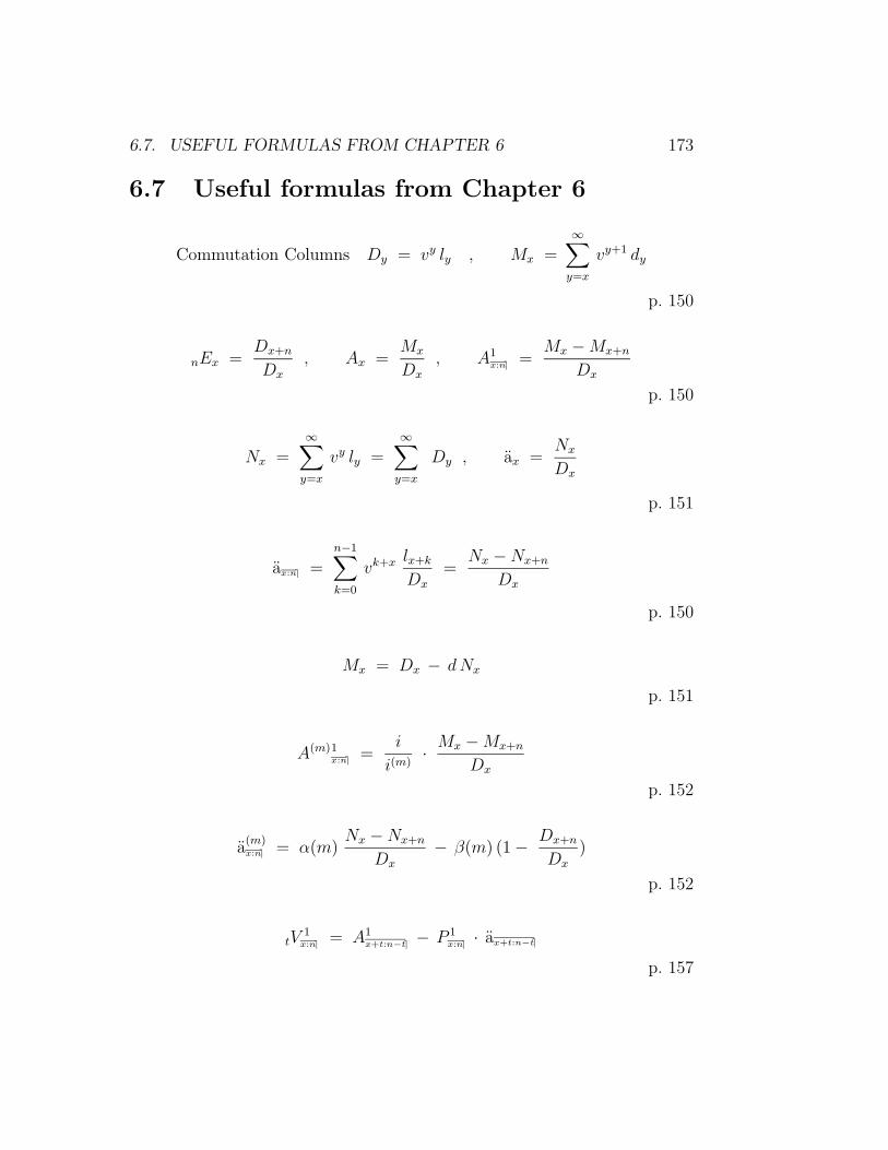
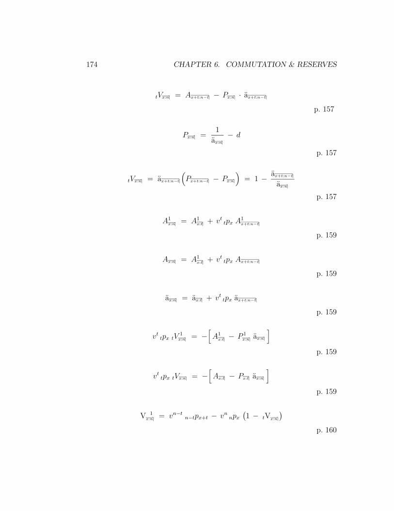
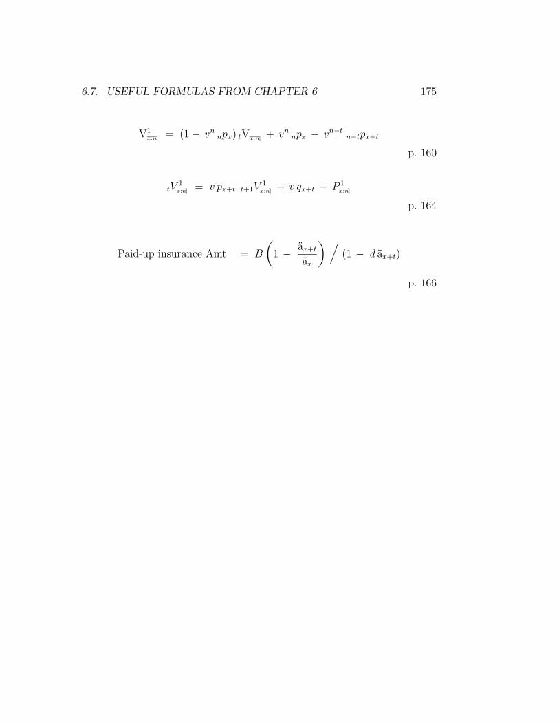
6.7 Useful formulas from Chapter 6

Commutation Columns Dy = vy ly , Mx =∞∑

y=x

vy+1 dy

p. 150

nEx =Dx+n

Dx

, Ax =Mx

Dx

, A1x:n⌉ =

Mx − Mx+n

Dx

p. 150

Nx =∞∑

y=x

vy ly =∞∑

y=x

Dy , ax =Nx

Dx

p. 151

ax:n⌉ =n−1∑

k=0

vk+x lx+k

Dx

=Nx − Nx+n

Dx

p. 150

Mx = Dx − dNx

p. 151

A(m)1x:n⌉ =

i

i(m)·

Mx − Mx+n

Dx

p. 152

a(m)x:n⌉ = α(m)

Nx − Nx+n

Dx

− β(m) (1 −Dx+n

Dx

)

p. 152

tV1

x:n⌉ = A1x+t:n−t⌉ − P 1

x:n⌉ · ax+t:n−t⌉

p. 157


tVx:n⌉ = Ax+t:n−t⌉ − Px:n⌉ · ax+t:n−t⌉

p. 157

Px:n⌉ =1

ax:n⌉

− d

p. 157

tVx:n⌉ = ax+t:n−t⌉

(

Px+t:n−t⌉ − Px:n⌉

)

= 1 −ax+t:n−t⌉

ax:n⌉

p. 157

A1x:n⌉ = A1

x:t⌉ + vttpx A1

x+t:n−t⌉

p. 159

Ax:n⌉ = A1x:t⌉ + vt

tpx Ax+t:n−t⌉

p. 159

ax:n⌉ = ax:t⌉ + vttpx ax+t:n−t⌉

p. 159

vttpx tV

1x:n⌉ = −

[

A1x:t⌉ − P 1

x:n⌉ ax:n⌉

]

p. 159

vttpx tVx:n⌉ = −

[

Ax:t⌉ − Px:t⌉ ax:n⌉

]

p. 159

V 1x:n⌉ = vn−t

n−tpx+t − vnnpx

(

1 − tVx:n⌉

)

p. 160

6.7. USEFUL FORMULAS FROM CHAPTER 6 175

V1x:n⌉ = (1 − vn

npx) tVx:n⌉ + vnnpx − vn−t

n−tpx+t

p. 160

tV1

x:n⌉ = v px+t t+1V1

x:n⌉ + v qx+t − P 1x:n⌉

p. 164

Paid-up insurance Amt = B

(

1 −ax+t

ax

)

/

(1 − d ax+t)

p. 166


Bibliography

[1] Bowers, N., Gerber, H., Hickman, J., Jones, D. and Nesbitt, C. Actu-arial Mathematics Society of Actuaries, Itasca, Ill. 1986

[2] Cox, D. R. and Oakes, D. Analysis of Survival Data, Chapman andHall, London 1984

[3] Feller, W. An Introduction to Probability Theory and its Ap-plications, vol. I, 2nd ed. Wiley, New York, 1957

[4] Feller, W. An Introduction to Probability Theory and its Ap-plications, vol. II, 2nd ed. Wiley, New York, 1971

[5] Gerber, H. Life Insurance Mathematics, 3rd ed. Springer-Verlag,New York, 1997

[6] Hogg, R. V. and Tanis, E. Probability and Statistical Inference,5th ed. Prentice-Hall Simon & Schuster, New York, 1997

[7] Jordan, C. W. Life Contingencies, 2nd ed. Society of Actuaries,Chicago, 1967

[8] Kalbfleisch, J. and Prentice, R. The Statistical Analysis of FailureTime Data, Wiley, New York 1980

[9] Kellison, S. The Theory of Interest. Irwin, Homewood, Ill. 1970

[10] Larsen, R. and Marx, M. An Introduction to Probability and itsApplications. Prentice-Hall, Englewood Cliffs, NJ 1985

[11] Larson, H. Introduction to Probability Theory and StatisticalInference, 3rd ed. Wiley, New York, 1982

177

178 BIBLIOGRAPHY

[12] Lee, E. T. Statistical Models for Survival Data Analysis, LifetimeLearning, Belmont Calif. 1980

[13] The R Development Core Team, R: a Language and Environment.

[14] Splus, version 7.0. MathSoft Inc., 1988, 1996, 2005

[15] Spiegelman, M. Introduction to Demography, Revised ed. Univ. ofChicago, Chicago, 1968

[16] Venables, W. and Ripley, B. Modern Applied Statistics with S, 4thed. Springer-Verlag, New York, 2002

Documents

Actuarial Mathematics and Life-Table Statisticsevs/s470/BookChaps/Chp6.pdf · Actuarial Mathematics and Life-Table Statistics Eric V. Slud Mathematics Department University of Maryland,