Embed Size (px)
Citation preview

Actuarial Mathematicsand Life-Table Statistics
Eric V. SludMathematics Department
University of Maryland, College Park
March 22, 2009

c©2009
Eric V. Slud
Statistics Program
Mathematics Department
University of Maryland
College Park, MD 20742

Contents
0.1 Preface . . . . . . . . . . . . . . . . . . . . . . . . . . . . . . . iv
1 Basics of Probability & Interest 1
1.1 Probabilities about Lifetimes . . . . . . . . . . . . . . . . . . . 1
1.1.1 Random Variables and Expectations . . . . . . . . . . 6
1.2 Theory of Interest . . . . . . . . . . . . . . . . . . . . . . . . . 9
1.2.1 Interest Rates and Compounding . . . . . . . . . . . . 9
1.2.2 Present Values and Payment Streams . . . . . . . . . . 14
1.2.3 Principal and Interest, and Discount Rates . . . . . . . 17
1.2.4 Variable Interest Rates . . . . . . . . . . . . . . . . . . 20
1.2.5 Continuous-time Payment Streams . . . . . . . . . . . 24
1.3 Exercise Set 1 . . . . . . . . . . . . . . . . . . . . . . . . . . . 25
1.4 Worked Examples . . . . . . . . . . . . . . . . . . . . . . . . . 28
1.5 Useful Formulas . . . . . . . . . . . . . . . . . . . . . . . . . . 31
2 Interest & Force of Mortality 33
2.1 More on Theory of Interest . . . . . . . . . . . . . . . . . . . . 33
2.1.1 Annuities & Actuarial Notation . . . . . . . . . . . . . 34
2.1.2 Loan Repayment: Mortgage, Bond, Sinking Fund . . . 39
i

ii CONTENTS
2.1.3 Loan Amortization & Mortgage Refinancing . . . . . . 41
2.1.4 Illustration on Mortgage Refinancing . . . . . . . . . . 42
2.1.5 Computational illustration in R . . . . . . . . . . . . . 44
2.2 Force of Mortality & Analytical Models . . . . . . . . . . . . . 48
2.2.1 Comparison of Forces of Mortality . . . . . . . . . . . . 55
2.3 Exercise Set 2 . . . . . . . . . . . . . . . . . . . . . . . . . . . 61
2.4 Worked Examples . . . . . . . . . . . . . . . . . . . . . . . . . 65
2.5 Useful Formulas from Chapter 2 . . . . . . . . . . . . . . . . . 69
3 Probability & Life Tables 73
3.1 Binomial Variables & Law of Large Numbers . . . . . . . . . . 74
3.1.1 Probability Bounds & Approximations . . . . . . . . . 77
3.2 Simulation of Discrete Lifetimes . . . . . . . . . . . . . . . . . 80
3.3 Expectation of Discrete Random Variables . . . . . . . . . . . 84
3.3.1 Rules for Manipulating Expectations . . . . . . . . . . 87
3.3.2 Curtate Expectation of Life . . . . . . . . . . . . . . . 90
3.4 Interpreting Force of Mortality . . . . . . . . . . . . . . . . . . 91
3.5 Interpolation Between Integer Ages . . . . . . . . . . . . . . . 92
3.5.1 Life Expectancy – Definition and Approximation . . . 96
3.6 Some Special Integrals . . . . . . . . . . . . . . . . . . . . . . 97
3.7 Exercise Set 3 . . . . . . . . . . . . . . . . . . . . . . . . . . . 100
3.8 Worked Examples . . . . . . . . . . . . . . . . . . . . . . . . . 103
3.9 Appendix on Large Deviation Probabilities . . . . . . . . . . . 109
3.10 Useful Formulas from Chapter 3 . . . . . . . . . . . . . . . . . 112
4 Expected Present Values of Payments 115

CONTENTS iii
4.1 Preliminaries . . . . . . . . . . . . . . . . . . . . . . . . . . . 116
4.2 Types of Contracts . . . . . . . . . . . . . . . . . . . . . . . . 118
4.2.1 Formal Relations, m = 1 . . . . . . . . . . . . . . . . . 121
4.2.2 Formulas for Net Single Premiums . . . . . . . . . . . 123
4.3 Extension to Multiple Payments per Year . . . . . . . . . . . . 125
4.4 Interpolation Formulas in Risk Premiums . . . . . . . . . . . . 130
4.5 Continuous Risk Premium Formulas . . . . . . . . . . . . . . . 132
4.5.1 Continuous Contracts & Residual Life . . . . . . . . . 133
4.5.2 Integral Formulas . . . . . . . . . . . . . . . . . . . . . 134
4.5.3 Risk Premiums under Theoretical Models . . . . . . . 136
4.5.4 Numerical Calculations of Life Expectancies . . . . . . 140
4.6 Exercise Set 4 . . . . . . . . . . . . . . . . . . . . . . . . . . . 144
4.7 Worked Examples . . . . . . . . . . . . . . . . . . . . . . . . . 148
4.8 Useful Formulas from Chapter 4 . . . . . . . . . . . . . . . . . 154
A General Features of Duration Data 157
A.1 Survival Data Concepts . . . . . . . . . . . . . . . . . . . . . . 158
A.2 Formal Notion of the Life Table . . . . . . . . . . . . . . . . . 162
A.2.1 The Cohort Life Table . . . . . . . . . . . . . . . . . . 163
A.3 Sample Spaces for Duration Data . . . . . . . . . . . . . . . . 165
A.3.1 Sample Space– Single Life . . . . . . . . . . . . . . . . 166
A.3.2 Sample Space – Cohort Population . . . . . . . . . . . 167
A.3.3 Sample Space – General Case . . . . . . . . . . . . . . 169
Bibliography 171

iv CONTENTS
0.1 Preface
This book is the text for an upper-level lecture course (STAT 470) at theUniversity of Maryland on actuarial mathematics, in particular on the basicsof Life Tables, Survival Models, and Life Insurance Premiums and Reserves.This is a ‘topics’ course, aiming not so much to prepare the students forspecific Actuarial Examinations – since it cuts across the Society of Actuaries’Exams FM, M (Segment MLC) and C – as to present the actuarial materialconceptually with reference to ideas from other undergraduate mathematicalstudies. Such a focus allows undergraduates with solid preparation in calculus(not necessarily mathematics or statistics majors) to explore their possibleinterests in business and actuarial science. It also allows the majority of suchstudents — who will choose some other avenue, from economics to operationsresearch to statistics, for the exercise of their quantitative talents — to knowsomething concrete and mathematically coherent about the topics and ideasactually useful in Insurance.
The Insurance material on contingent present values and life tables isdeveloped as directly as possible from calculus and common-sense notions,illustrated through word problems. Both the Interest Theory and Proba-bility related to life tables are treated as wonderful concrete applications ofthe calculus. The lectures require no background beyond a third semester ofcalculus, but the prerequisite calculus courses must have been solidly under-stood. It is a truism of pre-actuarial advising that students who have notdone really well in and digested the calculus ought not to consider actuarialstudies.
It is not assumed that the student has seen a formal introduction to prob-ability. Notions of relative frequency and average are introduced first withreference to the ensemble of a cohort life-table, the underlying formal randomexperiment being random selection from the cohort life-table population (or,in the context of probabilities and expectations for ‘lives aged x’, from thesubset of lx members of the population who survive to age x). The cal-culation of expectations of functions of a time-to-death random variables isrooted on the one hand in the concrete notion of life-table average, which isthen approximated by suitable idealized failure densities and integrals. Later,in discussing Binomial random variables and the Law of Large Numbers, thecombinatorial and probabilistic interpretation of binomial coefficients are de-

0.1. PREFACE v
rived from the Binomial Theorem, which the student the is assumed to knowas a topic in calculus (Taylor series identification of coefficients of a poly-nomial.) The general notions of expectation and probability are introduced,but for example the Law of Large Numbers for binomial variables is treated(rigorously) as a topic involving calculus inequalities and summation of finiteseries. This approach allows introduction of the numerically and conceptuallyuseful large-deviation inequalities for binomial random variables to explainjust how unlikely it is for binomial (e.g., life-table) counts to deviate muchpercentage-wise from expectations when the underlying population of trialsis large.
While the basics of actuarial Life Contingencies are treated elsewhere as aproblem-solving method using mortality tables presented in a cohort format,some effort is devoted in this book to contrasting the form in which theunderlying mortality data are received to the form of the cohort life tableused in calculating premiums and reserves. This allows statistics students toconnect the basic ideas of life table construction – considered by actuaries amore advanced topic – to the problems of statistical estimation. Accordingly,some material is included on statistics of biomedical studies and on reliabilitywhich would not ordinarily find its way into an actuarial course.
The reader is also not assumed to have worked previously with the The-ory of Interest. These lectures present Theory of Interest as a mathematicalproblem-topic, which is rather unlike what is done in typical finance courses.Getting the typical Interest problems — such as the exercises on mortgagerefinancing and present values of various payoff schemes — into correct for-mat for numerical answers is often not easy even for good mathematics stu-dents. The approach here is to return to the first principles of present-valueEquivalence and linear Superposition of payment streams over time. InterestTheory topics are presented here first as a way to learn the skills of apply-ing Equivalence and Superposition principles to real problems, but also asa way of highlighting the relationship between realized payouts under stan-dard Insurance contracts and instances of standard payment streams withrandom duration. In this approach, insurance reserves are seen as naturalgeneralizations of bond amortization schedules.
While the material in these lectures is presented systematically, it is notseparated by chapters into unified topics such as Interest Theory, ProbabilityTheory, Premium Calculation, etc. Instead the introductory material from

vi CONTENTS
probability and interest theory are interleaved, and later, various mathemat-ical ideas are introduced as needed to advance the discussion. No book atthis level can claim to be fully self-contained, but every attempt has beenmade to develop the mathematics to fit the actuarial applications as theyarise logically.
The coverage of the main body of each chapter is primarily ‘theoretical’.At the end of each chapter is an Exercise Set and a short section of WorkedExamples to illustrate the kinds of word problems which can be solved bythe techniques of the chapter. The Worked Examples sections show howthe ideas and formulas work smoothly together, and they highlight the mostimportant and frequently used formulas.
Finally, this book differs from other Actuarial texts in its use of compu-tational tools. Realistic problems on present values of payment streams, onprobabilistic survival models related to human lifetimes, and on insurance-contract premiums related to those models, rapidly lead to calculations toodifficult to do by hand or by calculator. Actuarial students often do thesecalculations using EXCEL or other spreadsheet programs, but the conceptu-ally based formulas often translate more effectively using mathematical toolsin computing platforms like MATLAB or the statistical language R, especiallywhere building blocks like root-finders or numerical integration routines areneeded. In this text, we encourage the students to use the free, open-source Rplatform because of its powerful tools for numerical integration, root-finding,life-table construction, and statistical estimation. Throughout this text, il-lustrations and Exercise solutions and solutions are given in terms of R.
Free web access to the downloadable R platform, including manuals, canbe found at http://www.r-project.org/. There are now many good in-troductory texts on computing with R in statistical applications. One textwhich combines a general introduction to R with the specifics of many sta-tistical data analysis methods, is Venables and Ripley (2002). Some goodfree tutorial material on R can also be found on the web, for example athttp://wiener.math.csi.cuny.edu/Statistics/R/simpleR/.

Chapter 1
Basics of Probability and theTheory of Interest
This first Chapter supplies some background on elementary Probability The-ory and basic Theory of Interest. The reader who has not previously studiedthese subjects may get an overview here, but will likely want to supplementthis Chapter with reading in any of a number of calculus-based introductionsto probability and statistics, such as Hogg and Tanis (2005) or Devore (2007),and the basics of the Theory of Interest as covered in the text of Kellison(2008) or Chapter 1 of Gerber (1997).
1.1 Probability, Lifetimes, and Expectation
In the cohort life-table model, imagine a number l0 of individuals bornsimultaneously and followed until death, resulting in data dx, lx for eachinteger age x = 0, 1, 2, . . ., where
lx = number of lives aged x (i.e. alive at birthday x )
anddx = lx − lx+1 = number dying between ages x, x + 1
Now, allow the age-variable to be denoted by t and to take all real values,not just whole numbers x, and treat S0(t) as the fraction of individuals in a
1

2 CHAPTER 1. BASICS OF PROBABILITY & INTEREST
life table surviving to exact age t. This nonincreasing function S0(t) wouldbe called the empirical ‘survivor’ or ‘survival’ function. Although it takes ononly rational values with denominator l0, it can be approximated by asurvival function S(t) which is continuous, decreasing, and continuouslydifferentiable (or piecewise continuously differentiable with just a few break-points) and takes values exactly = lx/l0 at integer ages x. Then for allpositive real y and t, S0(y)−S0(y + t) is the exact and S(y)−S(y + t)the approximated fraction of the initial cohort which fails between time yand y + t, and for integers x, k,
S(x) − S(x + k)
S(x)=
lx − lx+k
lx
denotes the fraction of those alive at exact age x who fail before x + k.
What do probabilities have to do with the cohort life table and survivalfunction ? To answer this, we first introduce probability as simply a relativefrequency, using numbers from a cohort life-table like that of the accompany-ing Illustrative Life Table. In response to a probability question, we supplythe fraction of the relevant life-table population, to obtain identities like
Pr(life aged 29 dies between exact ages 35 and 41 or between 52 and 60 )
=S(35) − S(41) + S(52) − S(60)
S(29)=
(l35 − l41) + (l52 − l60)/
l29
where our convention is that a life aged 29 is one of the cohort known tohave survived to the 29th birthday. Note that the event of dying betweenexact ages 35 and 41 or between 52 and 60 is the union of the nonoverlappingevents of the age random variable having value falling in the interval [35, 41)with that of falling in [52, 60).
The idea here is that all of the lifetimes covered by the life table areunderstood to be governed by an identical “mechanism” of failure, and thatany probability question about a single lifetime is really a question concerningthe fraction of a specified set of lives, e.g., those alive at age x, whoselifetimes will satisfy the stated property, e.g., who die either between 35 and41 or between 52 and 60. This “frequentist” notion of probability of an eventas the relative frequency with which the event occurs in a large populationof (independent) identical units is associated with the phrase “law of large

1.1. PROBABILITIES ABOUT LIFETIMES 3
numbers”, which will be discussed later. For now, remark only that the lifetable population should be large for the ideas presented so far to make goodsense. See Table 1.1 for an illustration of a cohort life-table with realisticnumbers, and for a cohort life table constructed to reflect the best estimatesof US male and female mortality rates in 2004, see the Social Security web-page http://www.ssa.gov/OACT/STATS/table4c6.html.
The main ideas arising in the discussion so far are really matters of com-mon sense when applied to relative frequency but require formal axioms whenused more generally:
• Probabilities are numbers between 0 and 1 assigned to subsets of theentire collection Ω of possible outcomes, with the probability of Ω it-self defined equal to 1. In the examples, the subsets which are assignedprobabilities include sub-intervals of the interval of possible human life-times measured in years, and also disjoint unions of such subintervals.These sets in the real line are viewed as possible events summarizingages at death of newborns in the cohort population. At this point, weregard each set A of ages as determining the subset of the cohortpopulation whose ages at death fall in A.
• The probability Pr(A ∪ B) of the union A ∪ B of disjoint (i.e.,nonoverlapping) sets A and B is necessarily equal to the sum of theseparate probabilities Pr(A) and Pr(B).
• When probabilities are requested with reference to a smaller universe ofpossible outcomes, such as B = lives aged 29, rather than all membersof a cohort population, the resulting conditional probabilities of eventsA are written Pr(A |B) and calculated as Pr(A∩B)/Pr(B), whereA ∩ B denotes the intersection or overlap of the two events A, B.The phrase “lives aged 29” defines an event which in terms of ages atdeath says simply “age at death is 29 or larger” or, in relation to thecohort population, specifies the subset of the population which survivesto exact age 29 (i.e., to the 29th birthday).
• Two events A, B are defined to be independent when Pr(A ∩ B) =Pr(A) · Pr(B) or — equivalently, as long as Pr(B) > 0 — whenthe conditional probability Pr(A|B) expressing the probability of Aif B were known to have occurred, is the same as the unconditionalprobability Pr(A).

4 CHAPTER 1. BASICS OF PROBABILITY & INTEREST
Table 1.1: Illustrative Life-Table, simulated to resemble realistic US Malelife-table up to age 78. For details of simulation, see Section 3.2 below.
Age x lx dx x lx dx
0 100000 2629 40 92315 2951 97371 141 41 92020 3322 97230 107 42 91688 4083 97123 63 43 91280 4144 97060 63 44 90866 4645 96997 69 45 90402 5326 96928 69 46 89870 5877 96859 52 47 89283 6808 96807 54 48 88603 7029 96753 51 49 87901 782
10 96702 33 50 87119 84111 96669 40 51 86278 88512 96629 47 52 85393 97413 96582 61 53 84419 108214 96521 86 54 83337 108815 96435 105 55 82249 121316 96330 83 56 81036 134417 96247 125 57 79692 142318 96122 133 58 78269 147619 95989 149 59 76793 157220 95840 154 60 75221 169621 95686 138 61 73525 178422 95548 163 62 71741 193323 95385 168 63 69808 202224 95217 166 64 67786 218625 95051 151 65 65600 226126 94900 149 66 63339 237127 94751 166 67 60968 242628 94585 157 68 58542 235629 94428 133 69 56186 270230 94295 160 70 53484 254831 94135 149 71 50936 267732 93986 152 72 48259 281133 93834 160 73 45448 276334 93674 199 74 42685 271035 93475 187 75 39975 284836 93288 212 76 37127 283237 93076 228 77 34295 283538 92848 272 78 31460 280339 92576 261

1.1. PROBABILITIES ABOUT LIFETIMES 5
Note: see a basic probability textbook, such as Hogg and Tanis (1997)or Devore (2007), for formal definitions and more detailed discussion of thenotions of sample space, event, probability, and conditional probability.
The life-table, and the mechanism by which members of the populationdie, are summarized first through the survivor function S(t) which at inte-ger values of t = x agrees with the ratios lx/l0. Note that S(t) has valuesbetween 0 and 1, and can be interpreted as the probability for a single indi-vidual to survive at least x time units. Since fewer people are alive at largerages, S(t) is a decreasing function of the continuous age-variable t, and inapplications S(t) should be continuous and piecewise continuously differen-tiable (largely for convenience, and because any analytical expression whichwould be chosen for S(t) in practice will be piecewise smooth). In addition,by definition, S(0) = 1. Another way of summarizing the probabilities ofsurvival given by this function is to define the density function
f(t) = − dS
dt(t) = −S ′(t) (1.1)
as the (absolute) rate of decrease of the function S. Then, by the funda-mental theorem of calculus, for any ages a < b,
Pr( life aged 0 dies between ages a and b )
= S(a) − S(b) =
∫ b
a
(−S ′(t)) dt =
∫ b
a
f(t) dt (1.2)
which has the very helpful geometric interpretation that the probability ofdying within the interval [a, b) is equal to the area under the density curvey = f(t) over the t-interval [a, b). Note also that the ‘probability’ rule whichassigns the integral
∫A
f(t) dt to the set A (which may be an interval,a union of intervals, or a still more complicated set) obviously satisfies thefirst two of the bulleted axioms displayed above, namely that P (Ω) = 1(where Ω is the sample space of all life-table outcomes) and Pr(A ∪ B) =Pr(A) + Pr(B) whenever A, B are disjoint or nonoverlapping subsets ofΩ.
The terminal age ω of a life table is an integer value large enough thatS(ω) is negligibly small, but no value S(t) for t < ω is zero. For practicalpurposes, no individual lives to the ω birthday. While ω is finite in reallife-tables and in some analytical survival models, most theoretical forms for

6 CHAPTER 1. BASICS OF PROBABILITY & INTEREST
S(t) have no finite age ω at which S(ω) = 0, and in those forms ω = ∞by convention.
In probability theory, the sample space Ω is the set of all detailed out-comes of the underlying data-generating experiment. Subsets of the samplespace to which probabilities will be assigned are called events. In this book,all of the interesting events concern lifetimes, or ages at death. Insurancecontract payouts will be expressed as functions of the lifetimes at death ofinsured lives, and the average or expected values of these payouts will be usedto calculate a fair equivalent value of the insurance contract to the insured.The machinery for calculating the average values relates to the concept ofrandom variable based on the sample space Ω = [0,∞) of lifetimes.
1.1.1 Random Variables and Expectations
Formally, a random variable is a real-valued mapping X defined on a samplespace Ω, such that s ∈ Ω : X(s) ∈ (a, b] is an event with assignedprobability whenever a < b are real numbers. The real number X(s)is interpreted as the value which would be observed if the detailed outcomeof the underlying random experiment were s ∈ Ω. The most importantfeature of a random variable is its probability distribution, which is theassignment rule of probabilities to all intervals (a, b] of values for X,denoted for all real numbers a ≤ b by
Pr(a < X ≤ b) ≡ Pr(s ∈ Ω : X(s) ∈ (a, b])
Remark 1.1 In datasets derived from actual mortality studies or insuranceportfolios, the detailed outcomes can be quite complicated, as discussed inAppendix A. However, in this and succeeding Chapters, we analyze lifetimesbased on the cohort life table model, also discussed in Appendix A, whichis a simplified model based on the reduced data-structure, in which numbersat risk and numbers of observed failures are tabulated on age intervals of oneyear.
Now we are ready to define some terms and motivate the notion of ex-pectation. Think of the age T at which a specified newly born member of

1.1. PROBABILITIES ABOUT LIFETIMES 7
the population will die as a random variable, which for present purposesmeans a variable which takes various values t with probabilities governed(at integer ages) by the life table data lx and the survivor function S(t) ordensity function f(t) in a formula like the one just given in equation (1.2).Suppose there is a contractual amount Y which must be paid (say, to theheirs of that individual) at the death of the individual at age T , and supposethat the contract provides a specific function Y = g(T ) according to whichthis payment depends on (the whole-number part of) the age T at whichdeath occurs. What is the average value of such a payment over all individ-uals whose lifetimes are reflected in the life-table ? Since dx = lx − lx+1
individuals (out of the original l0 ) die at ages between x and x + 1,thereby generating a payment g(x), the total payment to all individuals inthe life-table can be written as
∑
x
(lx − lx+1) g(x)
Thus the average payment, at least under the assumption that Y = g(T )depends only on the largest whole number [T ] less than or equal to T , is
∑x (lx − lx+1) g(x) / l0 =
∑x (S(x) − S(x + 1))g(x)
=∑
x
∫ x+1
xf(t) g(t) dt =
∫∞0
f(t) g(t) dt(1.3)
This quantity, the total contingent payment over the whole cohort divided bythe number in the cohort, is called the expectation of the random paymentY = g(T ) in this special case, and can be interpreted as the weighted averageof all of the different payments g(x) actually received, where the weightsare just the relative frequency in the life table with which those paymentsare received. More generally, if the restriction that g(t) depends only onthe integer part [t] of t were dropped , then the expectation of Y = g(T )would be given by the same formula
E(Y ) = E(g(T )) =
∫ ∞
0
f(t) g(t) dt (1.4)
The foregoing discussion of expectations based on lifetime random vari-ables included an interpretation of the expected value of discrete randomvariables in terms of weighted averages which holds much more generally. Inthis chapter, the averages are taken over all lives tabulated in an underly-ing cohort life table. In Chapter 3, specifically in Section 3.3, averages are

8 CHAPTER 1. BASICS OF PROBABILITY & INTEREST
taken over large samples of observations of discrete random variables. Withthe aid of the Law of Large Numbers, the weighted-average interpretation ofexpectations can be understood as a general mathematical result.
The displayed integral (1.4), like all expectation formulas, can be under-stood as a weighted average of values g(T ) obtained over a population,with weights equal to the probabilities of obtaining those values. Recall fromthe Riemann-integral construction in Calculus that the integral
∫f(t)g(t)dt
can be regarded approximately as the sum over very small time-intervals[t, t + ∆) of the quantities f(t)g(t)∆, quantities which are interpreted asthe base ∆ of a rectangle multiplied by its height f(t)g(t), and the rect-angle closely matches the area under the graph of the function f g over theinterval [t, t + ∆). The term f(t)g(t)∆ can alternatively be interpretedas the product of the value g(t) — essentially equal to any of the valuesg(T ) which can be realized when T falls within the interval [t, t + ∆) —multiplied by f(t)∆. The latter quantity is, by the Fundamental Theoremof the Calculus, approximately equal for small ∆ to the area under thefunction f over the interval [t, t + ∆), and is by definition equal to theprobability with which T ∈ [t, t + ∆). In summary, E(Y ) =
∫∞0
g(t)f(t)dtis the average of values g(T ) obtained for lifetimes T within small intervals[t, t+∆) weighted by the probabilities of approximately f(t)∆ with whichthose T and g(T ) values are obtained. The expectation is a weightedaverage because the weights f(t)∆ sum to the integral
∫∞0
f(t)dt = 1.
Remark 1.2 This way of approximating integrals of continuous integrandsby sums corresponding to the integrals of piecewise constant integrands isclosely related to the construction of the integral in terms of Riemann sums.For fuller details, see the definition the Integral via Riemann sums in a cal-culus book like Ellis and Gulick (2002).
The same idea and formula in (1.4) can be applied to the restricted popu-lation of lives aged x. The resulting quantity is then called the conditionalexpected value of g(T ) given that T ≥ x. The formula will be differentin two ways: first, the range of integrationis from x to ∞, because of theresitriction to individuals in the life-table who have survived to exact agex; second, the density f(t) must be replaced by f(t)/S(x), the so-calledconditional density given T ≥ x, which is found as follows. From the

1.2. THEORY OF INTEREST 9
definition of conditional probability, for t ≥ x,
Pr(t ≤ T < t + ∆ |T ≥ x) =Pr( t ≤ T < t + ∆ ∩ T ≥ x)
Pr(T ≥ x)
=Pr(t ≤ T < t + ∆)
Pr(T ≥ x)=
S(t)− S(t + ∆)
S(x)
Thus the density which can be used to calculate conditional probabilitiesPr(a ≤ T < b |T ≥ x) for x < a < b is
lim∆→0
1
∆Pr(t ≤ T < t+∆ |T ≥ x) = lim
∆→0
S(t)− S(t + ∆)
S(x)∆=
−S ′(t)
S(x)=
f(t)
S(x)
In other words, when it is desired to calculate the expectation of a functionY = g(T ) of the lifetime variable T only within the conditional or restrictedpopulation of individuals with lifetime ≥ x, then the density f(t) in theexpectation formula (1.4) should be replaced by the density which is equalto f(t)/S(x) for all values of t which are ≥ x, and which is 0 for valuest ∈ [0, x).
The result of all of this discussion of conditional expected values is theformula, with associated weighted-average interpretation:
E(g(T ) |T ≥ x) =1
S(x)
∫ ∞
x
g(t) f(t) dt (1.5)
1.2 Theory of Interest
1.2.1 Interest Rates and Compounding
Since payments based upon unpredictable occurrences or contingencies forinsured lives can occur at different times, we study next the Theory of Inter-est, which is concerned with valuing streams of payments made over time.The general model in the case of constant interest, to which we restrict inthe current sub-section, is as follows. Money is deposited in an account likea bank-account and grows according to a schedule determined by both theinterest rate and the occasions when interest amounts are compounded, that

10 CHAPTER 1. BASICS OF PROBABILITY & INTEREST
is, deemed to be added to the account. The compounding rules are impor-tant because they determine when new interest interest begins to be earnedon previously earned interest amounts.
The central concept of compound interest is that, over the fixed timeinterval of one year, an amount A0 deposited at the beginning of the intervalaccumulates to A1 = A0 · (1 + i) which could be withdrawn at the endof the interval. Since the constant interest rate is quoted as a constant overthe period of one year, we have 1 + i as the accumulation factor by whichan initial deposit is multiplied to find the balance at the end of one year.By convention, interest rates are generally quoted as annualized rates, whichmeans that the interest rate ih applied to a time-interval [t, t + h] for aperiod h of less than one year is prorated down to the interval h to givehih, which results in an accumulation factor 1 + hih. Thus, for an initialdeposit A0 at time t which is to be retained in a bank account for the timeh, so that the accumulated amount is compounded (i.e., is calculated bythe bank and owned by the depositor) at time t+ h, the balance which theowner could withdraw at time t + h is A(0) · (1 + hih).
If the quoted interest rate ih is annualized, and if interest earned isto be credited after every successive interval h = 1/m, then we say thatthe interest rate is a nominal annualized interest rate with m-times-yearly compounding or simply the nominal interest rate, and the standardnotation for it is i(m) instead of i1/m as written above.
Banks are not required to calculate interest from the instant (in practicalterms, the day) of deposit to the instant (i.e., the day) of withdrawal. Inpractice, the intervals of compounding are generally fractions h = 1/m ofa year, usually with m = 1, 2, 4, or 12. This means that after a depositof A0 at time t, the depositor wishing to withdraw the full accumulationor balance at time t + s for 0 < s < h owns only the initial amount A0,because no interest has yet been credited.
The further growth of deposited money over successive time intervalsof length h = 1/m, if compounded at each additional interval of length1/m, is easily understood inductively. With amount A0 deposited initiallyat time t, the balance as of time t + h is A0(1 + i(m)/m) and can beviewed as though it were simultaneously withdrawn and freshly deposited attime t + h, after which it would accumulate over the succeeding interval

1.2. THEORY OF INTEREST 11
[t + h, t + 2h] by multiplying the deposited amount A0(1 + i(m)/m) bythe interval-h accumulation factor 1 + i(m)/m. Thus the balance as of timet+2h = t+ 2/m is A0(1 + i(m)/m)2. Inductively, for k ≥ 2, if the balanceA0(1 + i(m)/m)k owned by the depositor at time t + k/m is regarded asinstantaneously withdrawn and redeposited as an initial balance for the nextinterval [t + k/m, t + (k + 1)/m], the balance at time t + (k + 1)/m isA0(1 + i(m)/m)k multiplied by the interval-h accumulation factor 1 + ih, orA0(1 + i(m)/m)(k+1).
The overall result of our reasoning about m-times yearly compoundednominal interest is the following:
Proposition 1.1 The accumulated value of an initial bank deposit of A0
compounded m times yearly at nominal interest rate i(m) after a timek/m+s, where 0 ≤ s < 1/m and k ≥ 0 is an integer, is (1+i(m)/m)k ·A0.
Proposition 1.1 with k = m says that at the annualized nominal interestrate i(m) , an initial deposit of A0 accumulates after exactly one yearto a balance of (1 + i(m)/m)m A0. Since the accumulation from the fullyear of deposit has the effect of multiplying the initial deposit by the factor(1 + i(m)/m)m, a factor which would have been 1 + i at interest rate icompounded yearly. This proves that the nominal interest rate i(m) with m-times-yearly compounding leads to exactly the same accumulation over wholeyears as a deposit account with the once-yearly compounded “effective” rate
i ≡ ieff = (1 + i(m)/m)m − 1
Since any nominal interest rate i(m) has its equivalent effective interestrate i = ieff providing the same yearly accumulations, the nominal interestrates i(m) with different values of m but the same value of i can alsobe regarded as equivalent. These whole-year-equivalent nominal rates aredetermined by solving the last equation for i(m) in terms of i = ieff :
i(m) = m(
(1 + i)1/m − 1)
(1.6)
For example, with i = .05, or 5% effective annual interest, the corre-sponding nominal rates i(m) for the most common values of m are obtainedthrough the R code line:

12 CHAPTER 1. BASICS OF PROBABILITY & INTEREST
mvec = c(1,2,4,12, 365) ; imvec = mvec*(1.05ˆ(1/mvec) - 1)
as
i(1) = .05 , i(2) = .04939 , i(4) = .04909 , i(12) = .04889 , i(365) = .04879
A few simple calculus manipulations allow us to establish the pattern ofthe displayed i(m) values for all choices of i, m. The right-hand side ofequation (1.6) is a function g(h) of h = 1/m, where
g(h) = h−1((1 + i)h − 1
)= (exp(h ln(1 + i))− 1)/h
has the form of a difference quotient from Calculus. Recall the Taylor seriesexpansion ez = 1 + z + z2/2 + z3/3! · · · which is valid for all z > 0.Substitute this series with z = h ln(1 + i) into the displayed formula forg(h) to conclude that
g(h) =∞∑
j=1
(ln(1 + i) · h)j
h · j!= ln(1 + i) +
∞∑
j=1
1
j!(ln(1 + i))j hj−1
is an increasing function of h > 0 and is always greater than its right-handlimit
g(0+) = limh0
exp(h ln(1 + i)) − 1
h=
d
dh
(eh ln(1+i)
)h=0
= ln(1 + i)
The information just established concerning the behavior of i(m) =g(1/m) as a function of m for fixed effective interest rate i = ieff issummarized as follows.
Proposition 1.2 When i = ieff is fixed, the nominal annual interest ratei(m) for m-times-yearly compounding is a decreasing function of the positiveinteger m and tends as m → ∞ to the limiting value, defined as the forceof interest,
δ = ln(1 + ieff) = limm→∞
i(m)
1.2. THEORY OF INTEREST 13
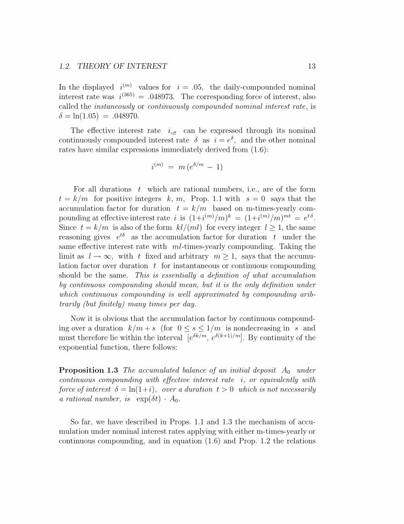
In the displayed i(m) values for i = .05, the daily-compounded nominalinterest rate was i(365) = .048973. The corresponding force of interest, alsocalled the instaneously or continuously compounded nominal interest rate, isδ = ln(1.05) = .048970.
The effective interest rate ieff can be expressed through its nominalcontinuously compounded interest rate δ as i = eδ, and the other nominalrates have similar expressions immediately derived from (1.6):
i(m) = m (eδ/m − 1)
For all durations t which are rational numbers, i.e., are of the formt = k/m for positive integers k, m, Prop. 1.1 with s = 0 says that theaccumulation factor for duration t = k/m based on m-times-yearly com-pounding at effective interest rate i is (1+i(m)/m)k = (1+i(m)/m)mt = et δ.Since t = k/m is also of the form kl/(ml) for every integer l ≥ 1, the samereasoning gives etδ as the accumulation factor for duration t under thesame effective interest rate with ml-times-yearly compounding. Taking thelimit as l → ∞, with t fixed and arbitrary m ≥ 1, says that the accumu-lation factor over duration t for instantaneous or continuous compoundingshould be the same. This is essentially a definition of what accumulationby continuous compounding should mean, but it is the only definition underwhich continuous compounding is well approximated by compounding arib-trarily (but finitely) many times per day.
Now it is obvious that the accumulation factor by continuous compound-ing over a duration k/m + s (for 0 ≤ s ≤ 1/m is nondecreasing in s andmust therefore lie within the interval [eδk/m, eδ(k+1)/m]. By continuity of theexponential function, there follows:
Proposition 1.3 The accumulated balance of an initial deposit A0 undercontinuous compounding with effective interest rate i, or equivalently withforce of interest δ = ln(1+i), over a duration t > 0 which is not necessarilya rational number, is exp(δt) · A0.
So far, we have described in Props. 1.1 and 1.3 the mechanism of accu-mulation under nominal interest rates applying with either m-times-yearly orcontinuous compounding, and in equation (1.6) and Prop. 1.2 the relations

14 CHAPTER 1. BASICS OF PROBABILITY & INTEREST
between nominal interest rates, force of interest, and effective interest rates.There is a further term for interest rates which must be disclosed to borrow-ers under US contracts, namely the Annual Percentage Rate or APR. Unlikethe interest rate terminology discussed up to this point, APR is a legal termwhich refers either (‘effective APR’) to the effective interest rate or (‘nominalAPR’ or simply ‘APR’) to the nominal interest, to which is added in eithercase the service fees charged by the lender as a fraction of the beginning-of-year loan balance. The APR disclosure is intended as a consumer protectionto the borrower, but may vary across jurisdictions in the way start-up fees(e.g., origination and participation) are required to be reported.
1.2.2 Present Values and Payment Streams
Applications of the theory of interest generally involve comparisons betweenstreams of payments which may be made at different times and may accu-mulate at different rates of interest. These payments may be deposits intoa bank or investment account, or loan repayments, or successive paymentsdesigned to accumulate over time at interest to a sufficient reserve fund tomeet some future liability.
First, a discrete payment stream is a sequence of (positive) depositamounts αj made at specified calendar times tj, j = 1, 2, . . . , n andwhich are regarded as accumulating from their times of deposit according toa schedule of interest rates r(t) which remain constant within successiveintervals of calendar time t but which may change from one such intervalto the next.
Two basic principles govern all problems of valuing such payment streams.
• The Principle of Equivalence defines equivalence at time τbetween two payment streams, one with payments and times (αj , tj,j = 1, 2, . . . , n) and interest rate function r(t) and the other withpayments and times (α∗
j , t∗j , j = 1, 2, . . . , n∗) and interest rate func-tion r∗(t), where τ ≥ maxj tj, maxj t∗j . These streams are calledequivalent at τ if the accumulated values at τ from the two paymentstreams under their respective interest rate functions are the same.

1.2. THEORY OF INTEREST 15
• The Principle of Linear Superposition states that the total accu-mulated amount resulting at time τ from a payment stream (αj , tj, j =1, 2, . . . , n) under interest rate function r(t) is the same as the sum ofthe accumulated values up to time T of n separate deposit accountsinitiated at the respective times tj with deposits of αj, all under thesame interest rate function r(t).
The two Principles as just stated do not yet tell us how to calculate theaccumulated values at τ under interest rate functions r(t) that vary overtime. However, we can already see that the first Principle is a definition,while we will see that the second is an essentially obvious restatement ofthe commutativity of addition together with the fact that the accumulationof discrete payment streams is a well-defined linear function of the paymentamounts αj.
Consider first the case where r(t) ≡ i is constant over the entire time-interval [minj tj, τ ]. Then Prop. 1.3 gives the contribution of the depositαj at time tj to the accumulated value at τ as αj · (1 + i)τ−tj . Onthe other hand, the direct inductive calculation of the accumulated amountsat all times tl ≥ tj due to the αj deposit, are also given via Prop. 1.3as αj · (1 + i)tl−tj , from which (by continuously compounding at interestrate i from the largest of the times tl until τ ) the final contributionof the αj deposit to the final accumulation at τ is again seen to beαj · (1 + i)τ−tj . This argument, with a little more notational effort and aninductive argument over the successively larger deposit times tl, can be madeinto a rigorous proof of the Linear Superposition principle in the constantinterest-rate environment with continuous compounding. The formula forthe continuously compounded accumulated value of the stream at time τ is
n∑
j=1
αj (1 + i)τ−tj =n∑
j=1
αj eδ (τ−tj) (1.7)
If compounding is instead m-times-yearly and all of the time-differences τ−tl
are integer multiples of 1/m, then we appeal to Propositions 1.1 and 1.3to confirm that there is no difference between the accumulated values ateffective interest rate i under continuous or m-times-yearly compounding,and formula (1.7) again expresses the accumulated value at τ , which is also

16 CHAPTER 1. BASICS OF PROBABILITY & INTEREST
equal ton∑
j=1
αj (1 + i(m)/m)m(τ−tj)
The most important application of the principle of equivalence is in find-ing a deposit amount αPV at a single fixed time t which is equivalentto the payment stream (αj, tj, j = 1, . . . , n) at all times τ ≥ maxj tj, atthe same effective interest rate i = ieff with continuous compounding asis used to accumulate (αj, tj, j = 1, . . . , n). This amount αPV is thencalled the present value of the payment stream at time t . To seewhy this is possible, consider any fixed τ ≥ max(t, maxj tj) and equatethe accumulated value (1.7) to the accumulated value αPV (1 + i)τ−t of thesingle deposit at time t using interest rate i, yielding:
n∑
j=1
αj (1 + i)τ−tj = αPV (1 + i)τ−t =⇒ αPV =n∑
j=1
αj (1 + i)t−tj
(1.8)This equation determining αPV evidently does not depend upon τ . It tellsfirst (with n = 1, t1 = 0 in (1.8)) the present value at fixed interest rate iof a payment of 1 exactly t years in the future, (1 + i)−t. This is theamount which must be put in the bank at time 0 in order to accumulate bythe factor (1 + i)t given by Prop. 1.3) to the value 1 at time t. Then, moregenerally,
the present value at time 0 under constant interest rate i ofa payment stream consisting of payments αj at future timestj, j = 1, . . . , n is equal to the summation
∑nj=1 αj (1 + i)−tj .
The same phenomenon, that a single deposit αPV at time t0 can beequivalent at all times τ to a payment stream (αj, tj, j = 1, . . . , n) turnsout to hold more generally whenever the same time-varying interest ratefunction r(t) is used to accumulate both the single deposit and the paymentstream. The proof of this Fact will be left to an Exercise in Section 1.2.4where accumulation formulas for variable interest rates are discussed. Themagnitude αPV is then the general present value of the payment stream attime t0.

1.2. THEORY OF INTEREST 17
1.2.3 Principal and Interest, and Discount Rates
In this Section, we consider the compounding of interest from the point ofview of a borrower of an amount L at time 0, where the interest rate isconstant with ieff = i. Initially assume continuous compounding for allaccumulations. If the borrower plans to make payments αj , 1 ≤ j ≤ n, attimes 0 < t1 < t2 < · · · < tn, then by definition
the principal remaining on the loan as of time t is equal to theaccumulated value at t of the single deposit L at time 0 , minusthe accumulated value at t under continuously compoundedeffective rate i of all payments made at times before t, i.e.,
Principal at time t = L (1 + i)t −∑
j: tj≤t αj (1 + i)t−tj .
The principal remaining in the loan just after a payment has been made isthe same as the amount the borrower could pay to pay off the loan completelyat that instant. In addition, if there are fees or late charges due at the timestj when payments are made, then those amounts are added to the Principalor Balance owed as of tj. However, in the present discussion we ignore allsuch additional fees or charges.
The principal owed on the loan just after time t reflects that as of timet, the lender must be compensated for the amount (1 + i)t L to which theoriginal loan amount would accumulate; while the accumulated value of thestream of payments actually made up to time t reduces the debt.
Each payment αj made can be broken down into the so-called Interestand Principal portions by the rule:
Interest Portion of Paymt at tj = (Principal at tj−1) · ((1 + i)tj−tj−1 − 1)
Principal Portion of Paymt at tj = αj − Interest Portion of Paymt at tj
The first of these lines is clearly the amount of interest that the principaljust after tj−1 would have earned at rate i over the time interval tj − tj−1.The amount of the payment at tj minus the amount of interest at tj is theamount by which the principal decreases from just after tj−1 to just aftertj. This simple Proposition is not quite obvious, but is easily shown by analgebraic rearrangement of terms, given as an Exercise.

18 CHAPTER 1. BASICS OF PROBABILITY & INTEREST
Exercise 1.A. Show that the foregoing definitions of Principal and PrincipalPortions of payments are compatible by deriving the following identity fromthe definitions. If Π(t) denotes the principal owed just after time t, andπj denotes the principal portion of the payment at tj, then
Π(tj−1) − πj = Π(tj) 2
The nominal interest rates i(m) for different periods of compounding wereseen in Prop. 1.2 to be related by the formulas
(1 + i(m)/m)m = 1 + i = 1 + ieff , i(m) = m(1 + i)1/m − 1
(1.9)
Similarly, interest can be said to be governed by the discount rates d(m) forvarious compounding periods, defined by
1 − d(m)/m = (1 + i(m)/m)−1
Solving the last equation for d(m) gives
d(m) = i(m)/(1 + i(m)/m) (1.10)
The idea of discount rates is that if an amount 1 is loaned out at interest,then the amount d(m)/m is the correct amount to be repaid at the beginningrather than the end of each fraction 1/m of the year, with repayment ofthe principal of 1 at the end of the year, in order to amount to the sameeffective interest rate. The reason is that, according to the definition, theamount 1−d(m)/m accumulates at nominal interest i(m) to (1−d(m)/m) ·(1 + i(m)/m) = 1 after a time-period of 1/m.
The quantities i(m) and d(m) are naturally introduced as the interestpayments which must be made respectively at the ends and the beginningsof successive time-periods of length 1/m in order that the principal owed ateach time j/m on an amount 1 borrowed at time 0 will always be 1. Todefine these terms and justify this assertion, consider first the simplest case,m = 1. If 1 is to be borrowed at time 0, then the single payment at time1 which fully compensates the lender, if that lender could alternatively haveearned interest rate i, is (1+i), which we view as a payment of 1 principal(the face amount of the loan) and i interest. In exactly the same way, if1 is borrowed at time 0 for a time-period 1/m, then the repayment at

1.2. THEORY OF INTEREST 19
time 1/m takes the form of 1 principal and i(m)/m interest. Thus, if1 was borrowed at time 0, an interest payment of i(m)/m at time 1/mleaves an amount 1 still owed, which can be viewed as an amount borrowedon the time-interval (1/m, 2/m]. Then a payment of i(m)/m at time2/m still leaves an amount 1 owed at 2/m, which is deemed borroweduntil time 3/m, and so forth, until the loan of 1 on the final time-interval((m−1)/m, 1] is paid off at time 1 with a final interest payment of i(m)/mtogether with the principal repayment of 1. The overall result which wehave just proved intuitively is:
1 at time 0 is equivalent to the stream of m payments ofi(m)/m at times 1/m, 2/m, . . . , 1 plus the payment of 1 attime 1.
Similarly, if interest is to be paid at the beginning of the period of theloan instead of the end, the interest paid at time 0 for a loan of 1 wouldbe d = i/(1 + i), with the only other payment a repayment of principal attime 1. To see that this is correct, note that since interest d is paid at thesame instant as receiving the loan of 1 , the net amount actually receivedis 1 − d = (1 + i)−1, which accumulates in value to (1 − d)(1 + i) = 1 attime 1. Similarly, if interest payments are to be made at the beginningsof each of the intervals (j/m, (j + 1)/m] for j = 0, 1, . . . , m − 1, witha final principal repayment of 1 at time 1, then the interest paymentsshould be d(m)/m. This follows because the amount effectively borrowed(after the immediate interest payment) over each interval (j/m, (j + 1)/m]is (1−d(m)/m), which accumulates in value over the interval of length 1/mto an amount (1 − d(m)/m)(1 + i(m)/m) = 1. So throughout the year-longlife of the loan, the principal owed at (or just before) each time (j +1)/m isexactly 1. The overall result concerning m-period-yearly discount interestis
1 at time 0 is equivalent to the stream of m payments ofd(m)/m at times 0, 1/m, 2/m, . . . , (m−1)/m plus the paymentof 1 at time 1.
A useful algebraic exercise to confirm the displayed assertions is:

20 CHAPTER 1. BASICS OF PROBABILITY & INTEREST
Exercise 1.B. Verify that the present values at time 0 of the paymentstreams with m interest payments in the displayed assertions are respectively
m∑
j=1
i(m)
m(1 + i)−j/m +(1 + i)−1 and
m−1∑
j=0
d(m)
m(1 + i)−j/m +(1 + i)−1
and that both are equal to 1. These identities are valid for all i > 0. 2
1.2.4 Variable Interest Rates
Now we formulate the generalization of these ideas to the case of non-constantinstantaneously varying, but known or observed, effective interest rate r(t)at time t , corresponding to the instantaneous continuously compoundednominal rate, or time-varying force of interest , δ(t) = ln(1+r(t)). Considerthe compounding of interest over successive intervals [b + kh, b + (k + 1)h],where h = 1/m for large m, there is an essentially constant principalamount over each interval of length 1/m. Since we assume the functionsr(t) and therefore ln(1+ δ(t)) are uniformly continuous in t, so that oververy short intervals [b + kh, b + (k + 1)h] with instantaneous compounding,the interest rate and its associated force of interest are essentially constant,with accumulation factor over the interval given by ehδ(kh). Therefore, if aninitial time b and duration τ > 0 are fixed and [mτ ] = [τ/h] denotes thelargest integer ≤ mτ , we find that the continuous compounding of interestover the time-interval [b, b + τ ] results in an overall accumulation factor ofapproximately
ehδ(b) ehδ(b+h) ehδ(b+2h) · · · ehδ(b+([τ/h]−1)h) exp(((τ − h[τ/h]) · δ(b + h[τ/h])
)
which has limit as m → ∞ equal to
exp(
limm
1
m
[mτ ]−1∑
k=0
δ(b + k/m))
= exp(∫ t
0
δ(b + s) ds)
The last step in this chain of equalities relates the concept of continuouscompounding to that of the Riemann integral. To specify continuous-timevarying interest rates in terms of instantaneous effective rates, we would

1.2. THEORY OF INTEREST 21
equate the last displayed formula for the accumulation factor over [b, b+ τ ]to
exp(∫ t
0
ln(1 + r(b + s)) ds)
Next consider the case of deposits α0, α1, . . . , αk, . . . , αn made at times0, h, . . . , kh, . . . , nh, where h = 1/m is the given compounding-period, andwherenominal annualized instantaneous interest-rates δ(kh) (with compounding-period h) apply to the accrual of interest on the interval [kh, (k + 1)h). Ifthe accumulated bank balance just after time kh is denoted by Bk , thenhow can the accumulated bank balance be expressed in terms of αj andδ(jh) ? Clearly
Bk+1 = Bk · eδ(kh)/m + αk+1 , B0 = α0
The preceding difference equation can be solved in terms of successive sum-mation and product operations acting on the sequences αj and δ(jh), asfollows. First define a function Ak to denote the accumulated bank balanceat time kh for a unit invested at time 0 and earning interest with instan-taneous nominal interest rates δ(jh) applying respectively over the wholecompounding-intervals [jh, (j + 1)h), j = 0, . . . , k − 1. Then by definition,Ak satisfies a homogeneous equation analogous to the previous one, whichtogether with its solution is given by
Ak+1 = Ak · eδ(kh)/m , A0 = 1, Ak =k−1∏
j=0
eδ(jh)/m
We now return to the idea of equivalent investments and present value ofa payment stream, as discussed in Section 1.2.2. Our object is to determine asingle deposit D at time 0 which is equivalent at time τ = nh to a streamof deposits αj, j = 0, 1, 2, . . . , n, where all amounts accumulate accordingto the continuously compounded instantaneous effective interest rate r(t)and associated force of interest δ(t) = ln(1 + r(t)). By approximating thecontinuous interest rate function r(t) by one which is constant on intervals[kh, (k + 1)h), we have just calculated that an amount 1 at time 0compounds to an accumulated amount An at time τ = nh. Therefore, anamount D at time 0 accumulates to D · An at time τ , and in particularD = 1/An at time 0 accumulates to 1 at time τ . Note, as in (1.8)

22 CHAPTER 1. BASICS OF PROBABILITY & INTEREST
of Section 1.2.2, this single equivalent deposit D would be the same if theaccumulations were valued at any other time τ ′ > nh. Thus the presentvalue of 1 at time τ = nh is 1/An . Now define Gk to be the presentvalue of the stream of payments αj at time jh for j = 0, 1, . . . , k. SinceBk was the accumulated value just after time kh of the same stream ofpayments, and since the present value at 0 of an amount Bk at time khis just Bk/Ak, we conclude
Gk+1 =Bk+1
Ak+1=
Bk exp(δ(km)/m)
Ak exp(δ(km)/m)+
αk+1
Ak+1, k ≥ 1 , G0 = α0
Thus Gk+1 − Gk = αk+1/Ak+1, and
Gk+1 = α0 +k∑
i=0
αi+1
Ai+1
=k+1∑
j=0
αj
Aj
In summary, we have simultaneously found the solution for the accumulatedbalance Bk just after time kh and for the present value Gk at time 0 :
Gk =k∑
i=0
αi
Ai, Bk = Ak · Gk , k = 0, . . . , n
The formulas just developed can be used to give the internal rate of returnr over the time-interval [0, τ ] of a unit investment which pays amount αk
at times tk, k = 0, . . . , n, 0 ≤ tk ≤ τ . This constant (effective) interestrate r is the one such that
n∑
k=0
sk
(1 + r
)−tk= 1
With respect to the constant interest rate r , the present value of a paymentαk at a time tk time-units in the future is αk · (1 + r)−tk . Therefore thestream of payments αk at times tk, (k = 0, 1, . . . , n) becomes equivalent,for the uniquely defined interest rate r, to an immediate (time-0) paymentof 1.

1.2. THEORY OF INTEREST 23
Exercise 1.C. As an illustration of the notion of effective interest rate, orinternal rate of return, suppose that you are offered an investment optionunder which an investment of 10, 000 made now is expected to pay 300yearly for 5 years (beginning 1 year from the date of the investment), and then800 yearly for the following five years, with the principal of 10, 000 returnedto you (if all goes well) exactly 10 years from the date of the investment (atthe same time as the last of the 800 payments. If the investment goesas planned, what is the effective interest rate you will be earning on yourinvestment ?
Solution. As in all calculations of effective interest rate, the present valueofthe payment-stream, at the unknown interest rate r = ieff, must be bal-anced with the value (here 10, 000) which is invested. (That is because theindicated payment stream is being regarded as equivalent to bank interest atrate r.) The balance equation in the Example is obviously
10, 000 = 3005∑
j=1
(1 + r)−j + 80010∑
j=6
(1 + r)−j + 10, 000 (1 + r)−10
The right-hand side can be simplified somewhat, in terms of the notationx = (1 + r)−5, to
300
1 + r
( 1 − x
1 − (1 + r)−1
)+
800x
(1 + r)
( 1 − x
1 − (1 + r)−1
)+ 10000x2
=1 − x
r(300 + 800x) + 10000x2 (1.11)
Setting this simplified expression equal to the left-hand side of 10, 000 doesnot lead to a closed-form solution, since both x = (1+r)−5 and r involve theunknown r. Nevertheless, we can solve the equation roughly by ‘tabulating’the values of the simplified right-hand side as a function of r ranging inincrements of 0.005 from 0.035 through 0.075. (We can guess that thecorrect answer lies between the minimum and maximum payments expressedas a fraction of the principal.) This tabulation yields:
r .035 .040 .045 .050 .055 .060 .065 .070 .075(1.11) 11485 11018 10574 10152 9749 9366 9000 8562 8320
From these values, we can see that the right-hand side is equal to 10, 000for a value of r falling between 0.05 and 0.055. Interpolating linearly to

24 CHAPTER 1. BASICS OF PROBABILITY & INTEREST
approximate the answer yields r = 0.050 + 0.005 ∗ (10000 − 10152)/(9749 −10152) = 0.05189, while an accurate equation-solver finds r = 0.05186. Forexample, the root-finding function in R is called uniroot , and the R code forcomputing the effective interest rate in this Example is:
Rsolv = function(r) x = (1+r)^(-5)
(1-x)*(300+800*x)/r + 10000*x^2 - 10000
uniroot(Rsolv, c(.035,.075))$root
[1] 0.05185676
1.2.5 Continuous-time Payment Streams
There is a completely analogous development for continuous-time depositstreams with continuous compounding. Suppose D(t) to be the rate perunit time at which savings deposits are made, so that if we take m to go to∞ in the previous discussion, we have D(t) = limm→∞ mα[mt], where [·]again denotes greatest-integer. Taking δ(t) to be the time-varying nominalinterest rate with continuous compounding, and B(t) to be the accumulatedbalance as of time t (analogous to the quantity B[mt] = Bk from before,when t = k/m), we replace the previous difference-equation by
B(t + h) = B(t) (1 + h δ(t)) + hD(t) + o(h)
where o(h) denotes a remainder such that o(h)/h → 0 as h → 0.Subtracting B(t) from both sides of the last equation, dividing by h, andletting h decrease to 0, yields a differential equation at times t > 0 :
B′(t) = B(t) δ(t) + D(t) , A(0) = α0 (1.12)
The method of solution of (1.12), which is the standard one from differentialequations theory of multiplying through by an integrating factor , again hasa natural interpretation in terms of present values. The integrating factor1/A(t) = exp(−
∫ t
0δ(s) ds) is the present value at time 0 of a payment of
1 at time t, and the quantity B(t)/A(t) = G(t) is then the present valueof the deposit stream of α0 at time 0 followed by continuous deposits atrate D(t). The ratio-rule of differentiation yields
G′(t) =B′(t)
A(t)− B(t)A′(t)
A2(t)=
B′(t) − B(t) δ(t)
A(t)=
D(t)
A(t)

1.3. EXERCISE SET 1 25
where the substitution A′(t)/A(t) ≡ δ(t) has been made in the third ex-pression. Since G(0) = B(0) = α0, the solution to the differential equation(1.12) becomes
G(t) = α0 +
∫ t
0
D(s)
A(s)ds , B(t) = A(t)G(t)
Finally, the formula can be specialized to the case of a constant unit-ratepayment stream ( D(x) = 1, δ(x) = δ = ln(1 + i), 0 ≤ x ≤ T ) withno initial deposit (i.e., α0 = 0). By the preceding formulas, A(t) =exp(t ln(1 + i)) = (1 + i)t, and the present value of such a payment streamis ∫ T
0
1 · exp(−t ln(1 + i)) dt =1
δ
(1 − (1 + i)−T
)
Recall that the force of interest δ = ln(1 + i) is the limiting value obtainedfrom the nominal interest rate i(m) using the difference-quotient representa-tion:
limm→∞
i(m) = limm→∞
exp((1/m) ln(1 + i)) − 1
1/m= ln(1 + i)
The present value of a payment at time T in the future is then
(1 +
i(m)
m
)−mT
= (1 + i)−T = exp(−δ T )
1.3 Exercise Set 1
The first homework set covers the basic definitions in two areas:(i) probability as it relates to events defined from cohort life-tables, includingthe theoretical machinery of population and conditional survival, distribu-tion, and density functions and the definition of expectation; (ii) the theoryof interest and present values, with special reference to the idea of incomestreams of equal value at a fixed rate of interest.
(1). For how long a time should $100 be left to accumulate at 5% interestso that it will amount to twice the accumulated value (over the same timeperiod) of another $100 deposited at 3% ?

26 CHAPTER 1. BASICS OF PROBABILITY & INTEREST
(2). Use a calculator or computer to answer the following numerically:
(a) Suppose you sell for $6,000 the right to receive for 10 years the amountof $1,000 per year payable quarterly (starting at the end of the first quarter).What effective rate of interest makes this a fair sale price ? (You will haveto solve numerically or graphically, or interpolate a tabulation, to find it.)
(b) $100 deposited 20 years ago has grown at interest to $235. Theinterest was compounded twice a year. What were the nominal and effectiveinterest rates ?
(c) How much should be set aside (the same amount each year) at thebeginning of each year for 10 years to amount to $1000 at the end of the 10thyear at the interest rate of part (b) ?
In the following problems, S(t) denotes the probability for a newbornin a designated population to survive to exact age t . If a cohort life tableis under discussion, then the probability distribution relates to a randomlychosen member of the newborn cohort.
(3). Assume that a population’s survival probability function is given byS(t) = 0.1(100 − t)1/2, for 0 ≤ t ≤ 100.
(a) Find the probability that a life aged 0 will die between exact ages 19and 36.
(b) Find the probability that a life aged 36 will die before exact age 51.
(4). For members of the poulation in Problem (3),
(a) Find the expected age at death of a newborn (life aged 0).
(b) Find the expected age at death of a life aged 20.
(5). Use the Illustrative Life-table (Table 1.1) to calculate the followingprobabilities. (In each case, assume that the indicated span of years runsfrom birthday to birthday.) Find the probability
(a) that a life aged 26 will live at least 30 more years;
(b) that a life aged 22 will die between ages 45 and 55;
(c) that a life aged 25 will die either before age 50 or after age 70.

1.3. EXERCISE SET 1 27
(6). In a special population, you are given the following facts:
(i) The probability that two independent lives, respectively aged 25 and45, both survive 20 years is 0.7.
(ii) The probability that a life aged 25 will survive 10 years is 0.9.
Then find the probability that a life aged 35 will survive to age 65.
(7). Suppose that you borrowed $1000 at 6% effective rate, to be repaidin 5 years in a lump sum, and that after holding the money idle for 1 yearyou invested the money and earned 8% effective for theremaining four years.What is the effective interest rate you earned (ignoring interest costs) over 5years on the $1000 which you borrowed ? Taking interest costs into account,what is the present value of your profit over the 5 years of the loan ? Alsore-do the problem if instead of repaying all principal and interest at the endof 5 years, you must make a payment of accrued interest at the end of 3years, with the additional interest and principal due in a single lump-sum atthe end of 5 years.
(8). Find the total present value at 5% APR of payments of $1 at the endof 1, 3, 5, 7, and 9 years and payments of $2 at the end of 2, 4, 6, 8, and 10years.
(9). Find the present value at time 0 at a 6% effective interest rate of aseries payments of 100 at times 1, 2, 3 and of 300 at times 6, 7, 8.
(10). Find the present value at time 0 of payments of 100 at ten successivetimes 1, 2, . . . , 10 if the instanteous effective interest rate applying at alltimes t in the time interval [0, 10] is r(t) = .07 − (.002)t.
(11). Find the internal rate of return (i.e., the equivaent constant effectiveinterest rate) over the time interval [0, 7] of an investment which pays bankinterest of 4% at times in [0, 5] if you make deposits of 1000 at each ofthe times t = 0, 2, 4, if the interest rate earned on the time interval [5, 7]is 6%, and if the total balance is withdrawn at time 7.
(12). (i) Find the payment amount K such that a loan of 10, 000 at a 7%effective annual interest rate is repaid in exactly three payments consistingof an amount K at times 1 and 3 years and of 2K at 5 years.

28 CHAPTER 1. BASICS OF PROBABILITY & INTEREST
(ii) After finding K in part (i), decompose each of the three loan repay-ment amounts K, K, 2K at respective times, 1, 3, 5 into their principaland interest portions.
1.4 Worked Examples
Example 1. How many years does it take for money to triple in value atinterest rate i ?
The equation to solve is 3 = (1 + i)t, so the answer is ln(3)/ ln(1 + i),with numerical answer given by
t =
22.52 for i = 0.0516.24 for i = 0.0711.53 for i = 0.10
Example 2. Suppose that a sum of $1000 is borrowed for 5 years at 5%,with interest deducted immediately in a lump sum from the amount borrowed,and principal due in a lump sum at the end of the 5 years. Suppose furtherthat the amount received is invested and earns 7%. What is the value of thenet profit at the end of the 5 years ? What is its present value (at 5%) asof time 0 ?
First, the amount received by the borrower at time 0 is1000 (1 − d)5 = 1000/(1.05)5 = 783.53, where d = .05/1.05, since theamount received should compound to precisely the principal of 1000 at 5%interest in 5 years. Next, the compounded value of 783.53 for 5 years at7% is 783.53 (1.07)5 = 1098.94, so the net profit at the end of 5 years, afterpaying off the principal of 1000, is 98.94. The present value of the profitought to be calculated with respect to the ‘going rate of interest’, which inthis problem is presumably the rate of 5% at which the money is borrowed,so is 98.94/(1.05)5 = 77.52.
Example 3. For the following small cohort life-table (first 3 columns) with 5age-categories, find the probabilities for all values of [T ], both uncondition-ally and conditionally for lives aged 2, and find the expectation of both [T ]and (1.05)−[T ]−1.

1.4. WORKED EXAMPLES 29
The basic information in the table is the first column lx of numberssurviving. Then dx = lx − lx+1 for x = 0, 1, . . . , 4. The random variableT is the life-length for a randomly selected individual from the age=0 cohort,and therefore Pr([T ] = x) = Pr(x ≤ T < x + 1) = dx/l0. The conditionalprobabilities given survivorship to age-category 2 are simply the ratios withnumerator dx for x ≥ 2 , and with denominator l2 = 65.
x lx dx Pr([T ] = x) Pr([T ] = x|T ≥ 2) 1.05−x−1
0 100 20 0.20 0 0.952381 80 15 0.15 0 0.907032 65 10 0.10 0.15385 0.863843 55 15 0.15 0.23077 0.827704 40 40 0.40 0.61538 0.783535 0 0 0 0 0.74622
In terms of the columns of this table, we evaluate from the definitions andformula (1.3)
E([T ]) = 0 · (0.20) + 1 · (0.15) + 2 · (0.10) + 3 · (0.15) + 4 · (0.40) = 2.4
E([T ] |T ≥ 2) = 2 · (0.15385) + 3 · (0.23077) + 4 · (0.61538) = 3.4615
E(1.05−[T ]−1) = 0.95238 · 0.20 + 0.90703 · 0.15 + 0.86384 · 0.10+
+0.8277 · 0.15 + 0.78353 · 0.40 = 0.8497
The expectation of [T ] is interpreted as the average per person in the cohortlife-table of the number of completed whole years before death. The quantity(1.05)−[T ]−1 can be interpreted as the present value at birth of a paymentof 1 to be made at the end of the year of death, and the final expectationcalculated above is the average of that present-value over all the individualsin the cohort life-table, if the going rate of interest is 5%.
Example 4. Suppose that the death-rates qx = dx/lx for integer ages x ina cohort life-table follow the functional form
qx =
4 · 10−4 for 5 ≤ x < 308 · 10−4 for 30 ≤ x ≤ 55
between the ages x of 5 and 55 inclusive. Find analytical expressions forS(x), lx, dx at these ages if l0 = 105, S(5) = .96.

30 CHAPTER 1. BASICS OF PROBABILITY & INTEREST
The key formula expressing survival probabilities in terms of death-ratesqx is:
S(x + 1)
S(x)=
lx+1
lx= 1 − qx
orlx = l0 · S(x) = (1 − q0)(1 − q1) · · · (1 − qx−1)
So it follows that for x = 5, . . . , 30,
S(x)
S(5)= (1 − .0004)x−5 , lx = 96000 · (0.9996)x−5
so that S(30) = .940446, and for x = 31, . . . , 55,
S(x) = S(30) · (.9992)x−30 = .940446 (.9992)x−30
The death-counts dx are expressed most simply through the precedingexpressions together with the formula dx = qx lx .

1.5. USEFUL FORMULAS 31
1.5 Useful Formulas from Chapter 1
S(x) =lxl0
, dx = lx − lx+1
p. 1
P (x ≤ T < x + k) = S(x) − S(x + k) =lx − lx+k
lx
p. 2
f(t) = −S ′(t) , S(y) − S(y + t) =
∫ y+t
y
f(s) ds
p. 5
E(
g(T )∣∣∣T ≥ x
)=
1
S(x)
∫ ∞
x
g(t) f(t) dt
p. 9
1 + i = 1 + ieff =
(1 +
i(m)
m
)m
=
(1 − d(m)
m
)−m
= eδ
p. 18

32 CHAPTER 1. BASICS OF PROBABILITY & INTEREST

Chapter 2
Theory of Interest andForce of Mortality
The parallel development of Interest and Probability Theory topics continuesin this Chapter. For application in Insurance, we are preparing to valueuncertain payment streams in which times of payment may also be uncertain.The interest theory allows us to express the present values of deterministic orcertain payment streams compactly, while the probability material preparesus to find and interpret average or expected values of present values expressedas functions of random lifetime variables.
This installment of the course covers: (a) further formulas and topics inthe pure (i.e., non-probabilistic) theory of interest, and (b) more discussionof lifetime random variables, in particular of force of mortality or hazard-rates, and theoretical families of life distributions.
2.1 More on Theory of Interest
In this Section, we define notations and find compact formulas for presentvalues of some standard payment streams. To this end, newly defined pay-ment streams are systematically expressed in terms of previously consideredones. There are two primary methods of manipulating one payment-streamto give another for the convenient calculation of present values:
33

34 CHAPTER 2. INTEREST & FORCE OF MORTALITY
• First, if one payment-stream can be obtained from a second one pre-cisely by delaying all payments by the same amount t of time, thenthe present value of the first one is vt multiplied by the present valueof the second.
• Second, if a payment-stream A can be obtained as the superposition ofpayment streams B and C, i.e., can be obtained by paying the sum ofthe timed payment amounts defining the streams B and C, then thepresent value of stream A is the sum of the present values of B and C.
The following subsection contains several useful applications of these meth-ods. For another simple illustration, see Worked Example 2 at the end of theChapter.
2.1.1 Annuities & Actuarial Notation
The general present value formulas above will now be specialized to the caseof constant (instantaneous) interest rate r(t) ≡ i ≡ eδ at all times t ≥ 0,and some very particular streams of payments sj at times tj, relatedto periodic premium and annuity payments. The effective interest rate isalways denoted by i = ieff , and as before the m-times-per-year equivalentnominal interest rate is denoted by i(m). Also, from now on the standardand convenient notation
v ≡ 1/(1 + i) = 1 /
(1 +
i(m)
m
)m
will be used for the present value of a payment of 1 one year later.
(i) If s0 = 0 and s1 = · · · = snm = 1/m in the discrete setting, wherem ≥ 1 denotes the number of payments per year, and tj = j/m, then thepayment-stream is called an immediate annuity, and its present value Gn
is given the notation a(m)n and is equal, by the geometric-series summation
formula, to
m−1nm∑
j=1
(1 +
i(m)
m
)−j
=(1 +
i(m)
m
)−1 1 − (1 + i(m)/m)−nm
m(1 − (1 + i(m)/m)−1)

2.1. MORE ON THEORY OF INTEREST 35
which shows that
a(m)n =
1 − ((1 + i(m)/m)−m)n
m (1 + i(m)/m − 1)=
1 − vn
i(m)(2.1)
All of these immediate annuity values, for fixed v, n but varying m, areroughly comparable because all involve a total payment of 1 per year.Formula (2.1) shows that all of the values a
(m)n differ only through the factors
i(m), which differ by only a few percent for varying m and fixed i, as shownin Table 2.1. Recall from formula (1.9) that i(m) = m(1 + i)1/m − 1.
If, instead of the payment stream defining the immediate annuity, s0 =1/m but snm = 0, then nm deposits of 1/m are made at an arithmeticprogression of times from 1/m to n inclusive, and the present value notation
changes to a(m)n . The payment stream is then called an annuity-due, and
the present valueis given by any of the equivalent formulas
a(m)n = (1 +
i(m)
m) a
(m)n =
1 − vn
m+ a
(m)n =
1
m+ a
(m)
n−1/m(2.2)
The first of these formulas recognizes the annuity-due payment-stream asidentical to the annuity-immediate payment-stream shifted earlier by thetime 1/m and therefore worth more by the accumulation-factor (1+i)1/m =1+ i(m)/m. The third expression in (2.2) represents the annuity-due streamas being equal to the annuity-immediate stream with the payment of 1/mat t = 0 added and the payment of 1/m at t = n removed. The finalexpression says that if the time-0 payment is removed from the annuity-due,the remaining stream coincides with the annuity-immediate stream consistingof nm − 1 (instead of nm) payments of 1/m.
In the limit as m → ∞ for fixed n, the notation an denotes thecontinuous annuity, that is, the present value of an annuity paid instanta-neously at constant unit rate, with the limiting nominal interest-rate whichwas shown in the previous chapter to be limm i(m) = i(∞) = δ. The limitingbehavior of the nominal interest rate can be seen rapidly from the formula
i(m) = m((1 + i)1/m − 1
)= δ · exp(δ/m) − 1
δ/m
since (ez − 1)/z converges to 1 as z → 0. Then by (2.1) and (2.2),
an = limm→∞
a(m)n = lim
m→∞a
(m)n =
1 − vn
δ(2.3)
36 CHAPTER 2. INTEREST & FORCE OF MORTALITY
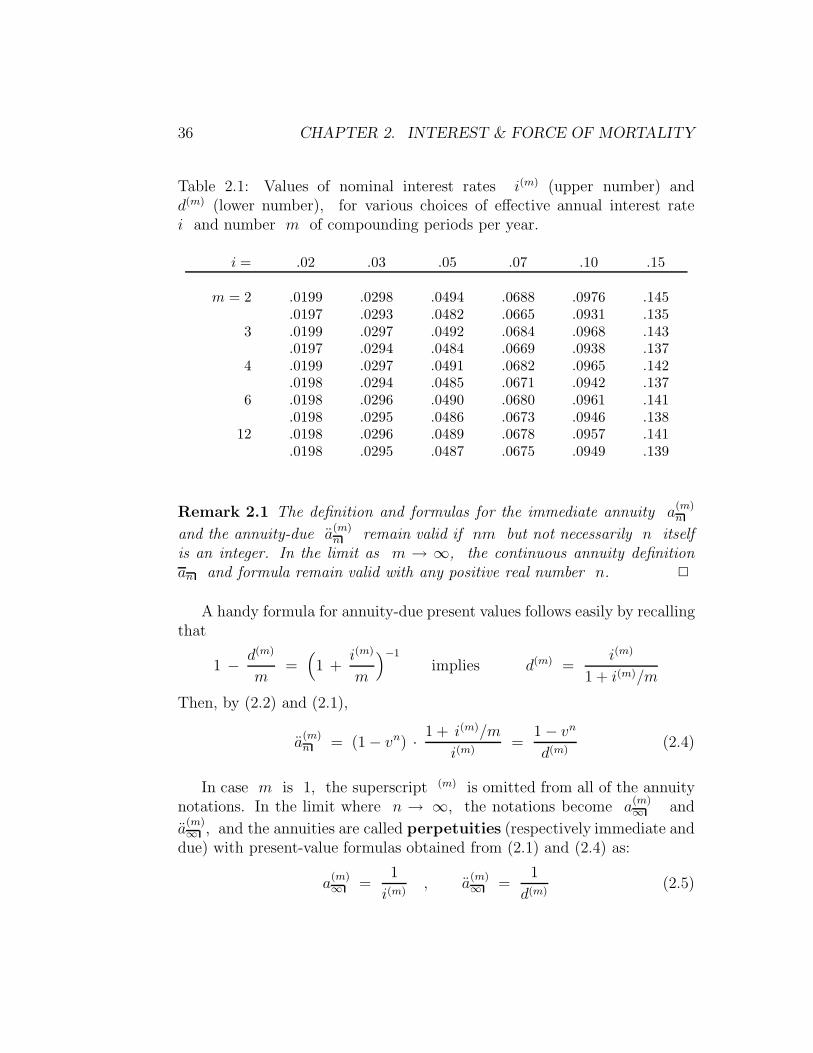
Table 2.1: Values of nominal interest rates i(m) (upper number) andd(m) (lower number), for various choices of effective annual interest ratei and number m of compounding periods per year.
i = .02 .03 .05 .07 .10 .15
m = 2 .0199 .0298 .0494 .0688 .0976 .145.0197 .0293 .0482 .0665 .0931 .135
3 .0199 .0297 .0492 .0684 .0968 .143.0197 .0294 .0484 .0669 .0938 .137
4 .0199 .0297 .0491 .0682 .0965 .142.0198 .0294 .0485 .0671 .0942 .137
6 .0198 .0296 .0490 .0680 .0961 .141.0198 .0295 .0486 .0673 .0946 .138
12 .0198 .0296 .0489 .0678 .0957 .141.0198 .0295 .0487 .0675 .0949 .139
Remark 2.1 The definition and formulas for the immediate annuity a(m)n
and the annuity-due a(m)n remain valid if nm but not necessarily n itself
is an integer. In the limit as m → ∞, the continuous annuity definitionan and formula remain valid with any positive real number n. 2
A handy formula for annuity-due present values follows easily by recallingthat
1 − d(m)
m=(1 +
i(m)
m
)−1
implies d(m) =i(m)
1 + i(m)/m
Then, by (2.2) and (2.1),
a(m)n = (1 − vn) · 1 + i(m)/m
i(m)=
1 − vn
d(m)(2.4)
In case m is 1, the superscript (m) is omitted from all of the annuitynotations. In the limit where n → ∞, the notations become a
(m)∞ and
a(m)∞ , and the annuities are called perpetuities (respectively immediate and
due) with present-value formulas obtained from (2.1) and (2.4) as:
a(m)∞ =
1
i(m), a
(m)∞ =
1
d(m)(2.5)

2.1. MORE ON THEORY OF INTEREST 37
We now build some more general annuity-related present values out ofthe standard functions a
(m)n and a
(m)n .
(ii). Consider first the case of the increasing perpetual annuity-due,
denoted (I(m)a)(m)∞ , which is defined as the present value of a stream of
payments (k + 1)/m2 at times k/m, for k = 0, 1, . . . forever. Clearly thepresent value is
(I(m)a)(m)∞ =
∞∑
k=0
m−2 (k + 1)(1 +
i(m)
m
)−k
Here are two methods to sum this series, the first purely mathematical, thesecond based on actuarial intuition. First, without worrying about the strictjustification for differentiating an infinite series term-by-term,
∞∑
k=0
(k + 1)xk =d
dx
∞∑
k=0
xk+1 =d
dx
x
1 − x= (1 − x)−2
for 0 < x < 1, where the geometric-series formula has been used to sumthe second expression. Therefore, with x = (1 + i(m)/m)−1 and 1 − x =(i(m)/m)/(1 + i(m)/m),
(I(m)a)(m)∞ = m−2
( i(m)/m
1 + i(m)/m
)−2
=
(1
d(m)
)2
=(a
(m)∞
)2
and (2.5) has been used in the last step. Another way to reach the same resultis to recognize the increasing perpetual annuity-due as 1/m multiplied by
the superposition of perpetuities-due a(m)∞ paid at times 0, 1/m, 2/m, . . . ,
and therefore its present value must be a(m)∞ · a(m)
∞ . As an aid in recognizing
this equivalence, consider each annuity-due a(m)∞ paid at a time j/m as
being equivalent to a stream of payments 1/m at time j/m, 1/m at(j + 1)/m, etc. Putting together all of these payment streams gives a totalof (k+1)/m paid at time k/m, of which 1/m comes from the annuity-duestarting at time 0, 1/m from the annuity-due starting at time 1/m, upto the payment of 1/m from the annuity-due starting at time k/m.
(iii). The increasing perpetual annuity-immediate (I(m)a)(m)∞ —
the same payment stream as in the increasing annuity-due, but deferred bya time 1/m — is related to the perpetual annuity-due in the obvious way
(I(m)a)(m)∞ = v1/m (I(m)a)
(m)∞ = (I(m)a)
(m)∞
/(1 + i(m)/m) =
1
i(m) d(m)

38 CHAPTER 2. INTEREST & FORCE OF MORTALITY
(iv). Now consider the increasing annuity-due of finite duration
n years. This is the present value (I(m)a)(m)n of the payment-stream of
(k + 1)/m2 at time k/m, for k = 0, . . . , nm− 1. Evidently, this payment-
stream is equivalent to (I(m)a)(m)∞ minus the sum of n multiplied by an
annuity-due a(m)∞ starting at time n together with an increasing annuity-
due (I(m)a)(m)∞ starting at time n. (To see this clearly, equate the payments
0 = (k + 1)/m2 − n · 1m
− (k − nm + 1)/m2 received at times k/m fork ≥ nm.) Thus
(I(m)a)(m)n = (I(m)a)
(m)∞
(1 − vn
)− na
(m)∞ vn
= a(m)∞
(a
(m)∞ − vn
[a
(m)∞ + n
] )
= a(m)∞
(a
(m)n − n vn
)
where, in the last line, recall that v = (1 + i)−1 = (1 + i(m)/m)−m and that
a(m)n = a
(m)∞ (1 − vn). The latter identity is easy to justify either by the
formulas (2.4) and (2.5) or by regarding the annuity-due payment stream as asuperposition of the payment-stream up to time n−1/m and the payment-stream starting at time n. As an exercise, fill in details of a second, intuitiveverification, analogous to the second verification in pargraph (ii) above.
(v). The decreasing annuity (D(m) a)(m)n is defined as (the present
value of) a stream of payments starting with n/m at time 0 and decreasingby 1/m2 after every time-period of 1/m, with no further payments at orafter time n. The easiest way to obtain the present value is through theidentity
(I(m)a)(m)n + (D(m)a)
(m)n = (n +
1
m) a
(m)n (2.6)
Again, as usual, the method of proving this is to observe that in the payment-stream whose present value is given on the left-hand side, the paymentamount at each of the times j/m, for j = 0, 1, . . . , nm − 1, is
j + 1
m2+ (
n
m− j
m2) =
1
m(n +
1
m)

2.1. MORE ON THEORY OF INTEREST 39
2.1.2 Loan Repayment: Mortgage, Bond, Sinking Fund
Perhaps the most common application of interest theory is the calculationof the payment amounts needed to repay a loan according to a few standardrepayment plans. In ordinary consumer purchases or long-term fixerd-rateloans on the purchase of a house, the usual repayment plan is a series of levelor equal payments made m times yearly (usually with m = 12, and usuallywith first payment at time 0) for a total duration of n years, so that at thelast payment (the nm’th payment, at time n− 1/m if the first payment wasmade at time 0) the loan has been completely paid off. We refer to this kindof repayment schedule with level payments as a mortgage loan. 1
Recall that the present value of a payment stream of amount c per year,with c/m paid at times 1/m, 2/m, . . . , n − 1/m, n/m, is c a
(m)n . Thus,
if an amount L has been borrowed for a term of n years, to be repaid byequal installments at the end of every period 1/m , at fixed nominal interestrate i(m), then the level payment c/m or installment payment amount
is obtained by equating L = c a(m)n
Mortgage Payment = L/(ma(m)n ) =
L i(m)
m (1 − vn)(2.7)
where v = 1/(1 + i) = (1 + i(m)/m)−m.
A second kind of plan to repay a loan is to pay equal amounts to cover onlythe interest amounts accrued every 1/m year on the principal for a durationof n years, with first payment made at time 1/m and last at time n, with theprincipal (the original amount borrowed) also repaid in a lump sum at timen. This arrangement is used by corporations or government agencies whichissue bonds: the borrowing agency receives the loan amount from investorsat time 0, called the face amount of the bond, and regularly issues interestpayments after every period of 1/m year (usually with m = 2 or 4), andfinally repays or redeems the face or principal amount of the bond at the endof the n year term of the bond. (The regular interest payments used to becalled coupon payments because of small paper coupons attached to the paperbond document, and which the investor would regularly redeem at a bank, atscheduled times, for the interest payment amount.) The reader should look
1In legal and historical terms, ‘mortgage’ refers to the way in which the promise torepay is secured by the house or other property purchased with the amount borrowed.

40 CHAPTER 2. INTEREST & FORCE OF MORTALITY
back to Section 1.2.3 where loan repayment amounts were formally brokendown into interest and principal portions, in order to confirm the sense of thisbond repayment plan. Since each payment by the borrower at times k/mfor k = 1, 2, . . . , nm (apart from the final lump sum principal repayment)consists of interest only (equal to the original face amount multiplied by(1 + i)1/m − 1 = i(m)/m), each of the intermediate payments contains 0principal portion, and the result of Exercise 1.A in Sec. 1.2.3 shows that theoriginal face amount or principal is also the principal or balance owed on theloan just after each interest payment, up to the final redemption when theprincipal is paid.
Now a corporation or governmental agency which borrows money frominvestors by issuing a bond, will often obligate itself through a formal legalarrangement to devote a certain category of income to a so-called sinkingfund, an investment account maintained by a trustee. Apart from the bondinterest payments at a contractual effective interst rate i made directly toinvestors (the lenders), the borrowing agency will also pay regular amountsat intervals of 1/m′ year to the sinking fund trustee for the same term of nyears as the bond, with the intention that the sinking fund will accumulateat its own possibly different investment interest rate i′ to the principal or faceamount of the issued bond at time n, at which time the principal is repaiddirectly to the bond investors. At (or just after) an intermediate times k/m,the amount built up in the sinking fund is referred to as a reserve towardthe ultimate redemption of the principal of the bond. We will see, later inthis book, that insurance reserves generalize these deterministic reserves toInsurances, where the future payouts are not determinstic but rather contin-gent on the mortality experience of the portfolio of insured lives.
Remark 2.2 Note that, if a borrowed amount L is repaid by regular interestpayments and a sinking fund, and if the number of payments per year intothe fund is m′ = m and the effective interest rate for the sinking fundis i′ = i, then evidently the sum of the regular m-times-yearly interest andsinking fund payment at each time k/m is precisely the same as the mortgagepayment (2.7). For m′ 6= m or i′ 6= i, a separate calculation is needed,leading to several exercises at the end of the Chapter. The following Exercisewith sketched solution gives an example.

2.1. MORE ON THEORY OF INTEREST 41
Exercise 2.A. A small city issues a bond for ten million dollars for ten yearsat 4% nominal quarterly interest (m = 4) and creates a sinking fund intowhich it will make annual deposits (m′ = 1), from tax receipts, on which itsfinancial advisors claim it can safely earn an effective annual rate of i′ = .055.Find the amount of the level annual sinking fund deposit.
Solution of Exercise 2.A. Since the interest payments are made at the con-tractual interest rate i (corresponding to i(4) = .04), the sinking fund mustappreciate to the loan amount of L = 107 at time t = 10. Therefore thesinking fund present value at time 10 (equal to its present value at t = 0accumulated by the factor (1 + i′)10 must be equated to L = 107. So theannual sinking fund deposit D is found through the equality
L = 107 = (1 + i′)10 · D a′10 = D
1 − (1.055)−10
.0551.05510
where a′ indicates that the annuity is calculated at interest rate i′.
2.1.3 Loan Amortization & Mortgage Refinancing
We analyze next the breakdown between principal and interest in repayinga mortgage loan by level payments (2.7). Of the payment made at time(k + 1)/m, how much can be attributed to interest and how much to princi-pal ? Consider the present value at time 0 of the debt for a unit (L = 1)loan amount less the accumulated amounts paid through time k/m :
1 − (ma(m)
k/m) / (ma
(m)n ) = 1 − 1 − vk/m
1 − vn=
vk/m − vn
1 − vn
The remaining debt, per unit of loan amount, valued just after time k/m,is denoted from now on by Bn, k/m. It is greater than the displayed presentvalue at 0 by a factor (1 + i)k/m, so is equal to
Bn, k/m = (1 + i)k/m vk/m − vn
1 − vn=
1 − vn−k/m
1 − vn(2.8)
The amount of interest for a loan amount of 1 after time 1/m is(1 + i)1/m − 1 = i(m)/m. Therefore the interest included in the payment at

42 CHAPTER 2. INTEREST & FORCE OF MORTALITY
(k + 1)/m is i(m)/m multiplied by the value Bn, k/m of outstanding debtjust after k/m. Thus the next total payment of i(m)/(m(1− vn)) consistsof the two parts
Amount of interest = m−1 i(m) (1 − vn−k/m)/(1 − vn)
Amount of principal = m−1i(m)vn−k/m/(1 − vn)
By definition, the principal included in each payment is the amount of thepayment minus the interest included in it. These formulas show in particularthat the amount of principal repaid in each successive payment increasesgeometrically in the payment number, which at first seems surprising. Noteas a check on the displayed formulas that the outstanding balance Bn,(k+1)/m
immediately after time (k + 1)/m is re-computed as Bn, k/m minus theinterest paid at (k + 1)/m, or
1 − vn−k/m
1 − vn− i(m)
m
vn−k/m
1 − vn=
1 − vn−k/m(1 + i(m)/m)
1 − vn
=1 − vn−(k+1)/m
1 − vn=(1 − a
(m)
(k+1)/m
/a
(m)n
)v−(k+1)/m (2.9)
as was derived above by considering the accumulated value of amounts paid.The general definition of the principal repaid in each payment is the excessof the payment over the interest since the past payment on the total balancedue immediately following that previous payment.
2.1.4 Illustration on Mortgage Refinancing
Suppose that a 30–year, nominal-rate 8%, $100, 000 mortgage payablemonthly is to be refinanced at the end of 8 years for an additional 15 years(instead of the 22 which would otherwise have been remaining to pay itoff) at 6%, with a refinancing closing-cost amount of $1500 and 2 points.(The points are each 1% of the refinanced balance including closing costs,and costs plus points are then extra amounts added to the initial balanceof the refinanced mortgage.) Suppose that the new pattern of payments isto be valued at each of the nominal interest rates 6%, 7%, or 8%, dueto uncertainty about what the interest rate will be in the future, and thatthese valuations will be taken into account in deciding whether to take outthe new loan.

2.1. MORE ON THEORY OF INTEREST 43
The monthly payment amount of the initial loan in this example was$100, 000(.08/12)/(1− (1+ .08/12)−360) = $733.76, and the present value asof time 0 (the beginning of the old loan) of the payments made through the
end of the 8th year is ($733.76) · (12a(12)
8) = $51, 904.69. Thus the present
value, as of the end of 8 years, of the payments still to be made under theold mortgage, is $(100, 000 − 51, 904.69)(1 + .08/12)96 = $91, 018.31. Thus,if the loan were to be refinanced, the new refinanced loan amount would be$91, 018.31 + 1, 500.00 = $92, 518.31. If 2 points must be paid in order tolock in the rate of 6% for the refinanced 15-year loan, then this amountis (.02)92518.31 = $1850.37 . The new principal balance of the refinancedloan is 92518.31 + 1850.37 = $94, 368.68, and this is the present value at anominal rate of 6% of the future loan payments, no matter what the term ofthe refinanced loan is. The new monthly payment (for a 15-year duration) ofthe refinanced loan is $94, 368.68(.06/12)/(1 − (1 + .06/12)−180) = $796.34.
For purposes of comparison, what is the present value at the currentgoing rate of 6% (nominal) of the continuing stream of payments underthe old loan ? That is a 22-year stream of monthly payments of $733.76,as calculated above, so the present value at 6% is $733.76 · (12a
(12)
22) =
$107, 420.21. Thus, if the new rate of 6% were really to be the correctone for the next 22 years, and each loan would be paid to the end of itsterm, then it would be a financial disaster not to refinance. Next, supposeinstead that right after re-financing, the economic rate of interest would bea nominal 7% for the next 22 years. In that case both streams of paymentswould have to be re-valued — the one before refinancing, continuing another22 years into the future, and the one after refinancing, continuing 15 years
into the future. The respective present values (as of the end of the 8th
year) at nominal rate of 7% of these two streams are:
Old loan: 733.76 (12a(12)
22) = $98, 700.06
New loan: 796.34 (12a(12)
15) = $88, 597.57
Even with these different assumptions, and despite closing-costs and points,it is well worth re-financing.

44 CHAPTER 2. INTEREST & FORCE OF MORTALITY
Exercise 2.B. Suppose that you can forecast that you will in fact sell yourhouse in precisely 5 more years after the time when you are re-financing. Atthe time of sale, you would pay off the cash principal balance, whatever itis. Calculate and compare the present values (at each of 6%, 7%, and 8%nominal interest rates) of your payment streams to the bank, (a) if youcontinue the old loan without refinancing, and (b) if you re-finance to geta 15-year 6% loan including closing costs and points, as described above.
2.1.5 Computational illustration in R
All of the calculations described above are very easy to program in any lan-guage from Fortran to Mathematica, and also on a programmable calculator;but they are also very handily organized within a spreadsheet, which seemsto be the way that MBA’s, bank-officials, and actuaries will learn to do themfrom now on.
In this section, an R function (cf. Venables & Ripley 2002) is provided todo some comparative refinancing calculations. Concerning the syntax of R,the only explanation necessary at this point is that * denotes multiplication,and ∧ denotes exponentiation.
The function RefExmp given below calculates mortgage payments, bal-ances for purposes of refinancing both before and after application of ad-ministrative costs and points, and the present value under any interest rate(not necessarily the ones at which either the original or refinanced loans aretaken out) of the stream of repayments to the bank up to and including thelump-sum payoff which would be made, for example, at the time of sellingthe house on which the mortgage loan was negotiated. The output of thefunction is a list which, in each numerical example below, is displayed in‘unlisted’ form, horizontally as a vector. Lines beginning with the symbol #are comment-lines.
The outputs of the function are as follows. Oldpayment is the monthlypayment on the original loan of face-amount Loan at nominal interest i(12) =OldInt for a term of OldTerm years. NewBal is the balance Bn, k/m of for-mula (2.8) for n = OldTerm, m = 12, and k/m = RefTim, and therefinanced loan amount is a multiple 1+ Points of NewBal, which is equalto RefBal + Costs. The new loan, at nominal interest rate NewInt, has

2.1. MORE ON THEORY OF INTEREST 45
R FUNCTION CALCULATING REFINANCE PAYMENTS & VALUES
RefExmp
function(Loan, OldTerm, RefTim, NewTerm, Costs, Points,
PayoffTim, OldInt, NewInt, ValInt)
# Function calculates present value of future payment stream
# underrefinanced loan.
# Loan = original loan amount;
# OldTerm = term of initial loan in years;
# RefTim = time in years after which to refinance;
# NewTerm = term of refinanced loan;
# Costs = fixed closing costs for refinancing;
# Points = fraction of new balance as additional costs;
# PayoffTim (no bigger than NewTerm) = time (from refinancing-
# time at which new loan balance is to be paid off in
# cash (eg at house sale);
# The three interest rates OldInt, NewInt, ValInt are
# nominal 12-times-per-year, and monthly payments
# are calculated.
vold = (1 + OldInt/12)^(-12)
Oldpaymt = ((Loan * OldInt)/12)/(1 - vold^OldTerm)
NewBal = (Loan * (1 - vold^(OldTerm - RefTim)))/
(1 - vold^OldTerm)
RefBal = (NewBal + Costs) * (1 + Points)
vnew = (1 + NewInt/12)^(-12)
Newpaymt = ((RefBal * NewInt)/12)/(1 - vnew^NewTerm)
vval = (1 + ValInt/12)^(-12)
Value = (Newpaymt * 12 * (1 - vval^PayoffTim))/ValInt +
(RefBal * vval^PayoffTim * (1 - vnew^(NewTerm -
PayoffTim)))/(1 - vnew^NewTerm)
list(Oldpaymt = Oldpaymt, NewBal = NewBal,
RefBal = RefBal, Newpaymt = Newpaymt, Value = Value)

46 CHAPTER 2. INTEREST & FORCE OF MORTALITY
monthly payments Newpaymt for a term of NewTerm years. The loan is tobe paid off PayoffTim years after RefTim when the new loan commences,and the final output of the function is the present value at the start of therefinanced loan with nominal interest rate ValInt of the stream of paymentsmade under the refinanced loan up to and including the lump sum payoff.
We begin our numerical illustration by reproducing the quantities calcu-lated in the previous subsection:
> unlist(RefExmp(100000, 30, 8, 15, 1500, 0.02, 15,
0.08, 0.06, 0.06))
Oldpaymt NewBal RefBal Newpaymt Value
733.76 91018 94368 796.33 94368
Note that, since the payments under the new (refinanced) loan are herevalued at the same interest rate as the loan itself, the present value Value ofall payments made under the loan must be equal to the the refinanced loanamount RefBal.
The comparisons of the previous Section between the original and refi-nanced loans, at (nominal) interest rates of 6, 7, and 8 %, are all recapitulatedeasily using this function. To use it, for example, in valuing the old loan at7%, the arguments must reflect a ‘refinance’ with no costs or points for aperiod of 22 years at nominal rate 6%, as follows:
> unlist(RefExmp(100000,30,8,22,0,0,22,0.08,0.08,0.07))
Oldpaymt NewBal RefBal Newpaymt Value
733.76 91018 91018 733.76 98701
(The small discrepancies between the values found here and in the previoussubsection are due to the rounding used there to express payment amountsto the nearest cent.)
We consider next a numerical example showing break-even point for refi-nancing by balancing costs versus time needed to amortize them.
Suppose that you have a 30-year mortage for $100,000 at nominal ratei(12) = 9%, with level monthly payments, and that after 7 years of paymentsyou refinance to obtain a new 30-year mortgage at 7% nominal interest ( =

2.1. MORE ON THEORY OF INTEREST 47
i(m) for m = 12), with closing costs of $1500 and 4 points (i.e., 4% of thetotal refinanced amount including closing costs added to the initial balance),also with level monthly payments. Figuring present values using the newinterest rate of 7%, what is the time K (to the nearest month) such thatif both loans — the old and the new — were to be paid off in exactly Kyears after the time (the 7-year mark for the first loan) when you would haverefinanced, then the remaining payment-streams for both loans from the timewhen you refinance are equivalent (i.e., have the same present value fromthat time) ?
We first calculate the present value of payments under the new loan.As remarked above in the previous example, since the same interest rate isbeing used to value the payments as is used in figuring the refinanced loan,the valuation of the new loan does not depend upon the time K to payoff.(It is figured here as though the payoff time K were 10 years.)
> unlist(RefExmp(1.e5, 30,7,30, 1500,.04, 10, 0.09,0.07,0.07))
Oldpaymt NewBal RefBal Newpaymt Value
804.62 93640 98946 658.29 98946
Next we compute the value of payments under the old loan, at 7% nominalrate, also at payoff time K = 10. For comparison, the value under theold loan for payoff time 0 (i.e., for cash payoff at the time when refinancingwould have occurred) coincides with the New Balance amount of $93640.
> unlist(RefExmp(1.e5, 30,7,23, 0,0, 10, 0.09,0.09,0.07))
Oldpaymt NewBal RefBal Newpaymt Value
804.62 93640 93640 804.62 106042
The values found in the same way when the payoff time K is successivelyreplaced by 4, 3, 3.167, 3.25 are 99979, 98946, 98593, 98951. Thus, thepayoff-time K at which there is essentially no difference in present valueat nominal 7% between the old loan or the refinanced loan with costs andpoints (which was found to have Value 98946), is 3 years and 3 monthsafter refinancing.

48 CHAPTER 2. INTEREST & FORCE OF MORTALITY
2.2 Force of Mortality & Analytical Models
Up to now, the function S(t) called the survivor or survival function hasbeen defined to be equal to the life-table ratio lx/l0 at all integer ages t = x,and to be piecewise continuously differentiable for all positive real values oft. Intuitively, for all positive real y and t, S(y)−S(y + t) is the fractionof the initial life-table cohort which dies between ages y and y + t, and(S(y)−S(y + t))/S(y) represents the fraction of those alive at exact age ywho fail before y + t. An equivalent representation is S(y) =
∫∞y
f(t) dt ,
where f(t) ≡ −S ′(t) is called the failure density. If T denotes the randomvariable which is the age at death for a newly born individual governed bythe same causes of failure as the life-table cohort, then Pr(T ≥ y) = S(y),and according to the Fundamental Theorem of Calculus,
limε→0+
P (y ≤ T ≤ y + ε)
ε= lim
ε→0+
1
ε
∫ y+ε
y
f(t) dt = f(y)
as long as the failure density is a continuous function.
Two further useful actuarial notations, often used to specify the theoret-ical lifetime distribution, are:
tpy = P(T ≥ y + t |T ≥ y
)= S(y + t)/S(y)
and
tqy = 1 − tpy = P(T ≤ y + t |T ≥ y
)= (S(y) − S(y + t))/S(y)
The quantity tqy is referred to as the age-specific death rate for periodsof length t. In the most usual case where t = 1 and y = x is an integer,the notation 1qx is replaced by qx, and 1px is replaced by px. Therate qx would be estimated from the cohort life table as the ratio dx/lx ofthose who die between ages x and x+1 as a fraction of those who reachedage x. The way in which this quantity varies with x is one of the mostimportant topics of study in actuarial science. For example, one importantway in which numerical analysis enters actuarial science is that one wishesto interpolate the values 1qy smoothly as a function of y. The topic called“Graduation Theory” among actuaries is the mathematical methodology ofInterpolation and Spline-smoothing applied to the raw function qx = dx/lx.

2.2. FORCE OF MORTALITY & ANALYTICAL MODELS 49
To give some idea what a realistic set of death-rates looks like, Figure 2.1pictures the age-specific 1-year death-rates qx for the simulated life-tablegiven as Table 1.1 on page 4. Additional granularity in the death-rates canbe seen in Figure 2.2, where the logarithms of death-rates are plotted. Aftera very high death-rate during the first year of life (26.3 deaths per thousandlive births), there is a year-by-year decline in death-rates roughly from 1.45per thousand in the second year to 0.34 per thousand in the eleventh year.(But there were small increases in rate from ages 4 to 7 and from 8to 9, which are as likely due to statistical irregularity as to real increasesin risk.) Between ages 11 and 40, there is an erratic but roughly linearincrease of death-rates per thousand from 0.4 to 3.0. However, at agesbeyond 40 there is a rapid increase in death-rates as a function of age.As can be seen from Figure 2.2, the values qx seem to increase roughlyas a power cx where c ∈ [1.08, 1.10]. (Compare this behavior with theGompertz-Makeham Example (v) below.) This exponential behavior of theage-specific death-rate for large ages suggests that the death-rates picturedcould reasonably be extrapolated to older ages using the formula
qx ≈ q78 · (1.0885)x−78 , x ≥ 79 (2.10)
where the number 1.0885 was found as log(q78/q39)/(78 − 39).
Now consider the behavior of εqx as ε gets small. It is clear that εqx
must also get small, roughly proportionately to ε, since the probability ofdying between ages x and x + ε is approximately ε f(x) when ε getssmall.
Definition: The limiting death-rate εqx/ε per unit time as ε 0 iscalled by actuaries the force of mortality µ(x). In reliability theory orbiostatistics, the same function is called the failure intensity, failure rate, orhazard intensity.
The reasoning above shows that for small ε,
εqy
ε=
1
εS(y)
∫ y+ε
y
f(t) dt −→ f(y)
S(y), ε 0
Thus
µ(y) =f(y)
S(y)=
−S ′(y)
S(y)= − d
dyln(S(y))

50 CHAPTER 2. INTEREST & FORCE OF MORTALITY
•
• • • • • • • • • • • • • • • • • • • • • • • • • • • • • • • • • • • • • • • • • • • • • • • • • • • • • ••• • • •
•••••••• •
• •
•
•••
•
•
•
•
Age-Specific Death Rates for Illustrative Life Table
Age in Years
Age
-Spe
cific
Dea
th R
ate
0 20 40 60 80
0.0
0.02
0.04
0.06
0.08
Figure 2.1: Plot of age-specific death-rates qx versus x, for the simulatedillustrative life table given in Table 1.1, page 4.

2.2. FORCE OF MORTALITY & ANALYTICAL MODELS 51
•
•
•
• • • •
• • •
••••
•••
• •• •
•• • • • •
• ••• • • •
• •• •
• •••• •
•• •
• •• • • •
• ••• • • • • • • •
• • • • •• • • • • •
• • • •
Logarithm of Death-Rates versus Age
Age in years
log(
Dea
th r
ate)
0 20 40 60 80
-8-7
-6-5
-4-3
for Illustrative Simulated Life-Table
Figure 2.2: Plot of logarithm log(qx) of age-specific death-rates as a functionof age x, for the simulated illustrative life table given in Table 1.1, page 4.The rates whose logarithms are plotted here are the same ones shown inFigure 2.1.

52 CHAPTER 2. INTEREST & FORCE OF MORTALITY
where the chain rule for differentiation was used in the last step. Replacingy by t and integrating both sides of the last equation between 0 and y,we find ∫ y
0
µ(t) dt =(− ln(S(t))
)y
0= − ln(S(y))
since S(0) = 1. Similarly,
∫ y+t
y
µ(s) ds = lnS(y)− lnS(y + t)
Now exponentiate to obtain the useful formulas
S(y) = exp−∫ y
0
µ(t) dt
, tpy =S(y + t)
S(y)= exp
−∫ y+t
y
µ(s) ds
Examples:
(i) If S(t) = (ω − t)/ω for 0 ≤ t ≤ ω (the uniform failure distributionon [0, ω] ), then µ(t) = (ω − t)−1. Note that this hazard function increasesto ∞ as t increases to ω.
(ii) If S(t) = e−µt for t ≥ 0 (the exponential failure distribution on[0,∞) ), then µ(t) = µ is constant.
(iii) If S(t) = exp(−λtγ) for t ≥ 0, then mortality follows the Weibulllife distribution model with shape parameter γ > 0 and scale parameter λ.The force of mortality takes the form
µ(t) = λ γ tγ−1
This model is very popular in engineering reliability. It has the flexibilitythat by choice of the shape parameter γ one can have
(a) (γ > 1) failure rate increasing as a function of x
(b) ( γ = 1) constant failure rate (exponential model), or
(c) (0 < γ < 1) decreasing failure rate.

2.2. FORCE OF MORTALITY & ANALYTICAL MODELS 53
But what one cannot have, in the examples considered so far, is a force-of-mortality function which decreases on part of the time-axis and increaseselsewhere.
(iv) Two other models for positive random variables which are popularin various statistical applications are the Gamma, with
S(y) =
∫ ∞
y
βα tα−1 e−βt dt /
∫ ∞
0
zα−1 e−z dz , α, β > 0
and the Lognormal, with
S(y) = 1 − Φ( ln y −m
σ
), m real, σ > 0
where
Φ(z) ≡ 1
2+
∫ z
0
e−u2/2 du√2π
is called the standard normal distribution function. In the Gamma case,the expected lifetime is α/β, while in the Lognormal, the expectation isexp(m + σ2/2). Neither of these last two examples has a convenient orinterpretable force-of-mortality function.
Increasing force of mortality intuitively corresponds to aging, where thecauses of death operate with greater intensity or effect at greater ages. Con-stant force of mortality, which is easily seen from the formula S(y) =exp(−
∫ y
0µ(t) dt) to be equivalent to exponential failure distribution, would
occur if mortality arose only from pure accidents unrelated to age. Decreas-ing force of mortality, which really does occur in certain situations, reflectswhat engineers call “burn-in”, where after a period of initial failures due toloose connections and factory defects the nondefective devices emerge andexhibit high reliability for a while. The decreasing force of mortality reflectsthe fact that the devices known to have functioned properly for a short whileare known to be correctly assembled and are therefore highly likely to have astandard length of operating lifetime. In human life tables, infant mortalitycorresponds to burn-in: risks of death for babies decrease markedly after theone-year period within which the most severe congenital defects and diseasesof infancy manifest themselves. Of course, human life tables also exhibit anaging effect at high ages, since the high-mortality diseases like heart diseaseand cancer strike with greatest effect at higher ages. Between infancy and
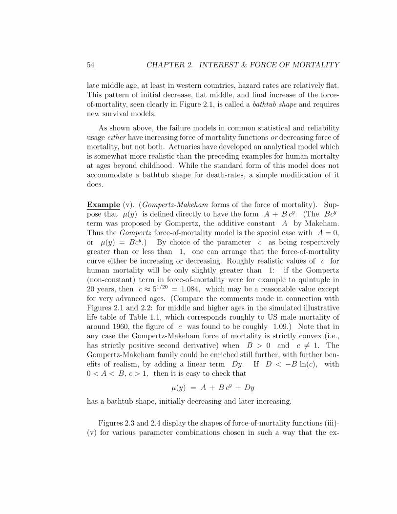
54 CHAPTER 2. INTEREST & FORCE OF MORTALITY
late middle age, at least in western countries, hazard rates are relatively flat.This pattern of initial decrease, flat middle, and final increase of the force-of-mortality, seen clearly in Figure 2.1, is called a bathtub shape and requiresnew survival models.
As shown above, the failure models in common statistical and reliabilityusage either have increasing force of mortality functions or decreasing force ofmortality, but not both. Actuaries have developed an analytical model whichis somewhat more realistic than the preceding examples for human mortaltyat ages beyond childhood. While the standard form of this model does notaccommodate a bathtub shape for death-rates, a simple modification of itdoes.
Example (v). (Gompertz-Makeham forms of the force of mortality). Sup-pose that µ(y) is defined directly to have the form A + B cy. (The Bcy
term was proposed by Gompertz, the additive constant A by Makeham.Thus the Gompertz force-of-mortality model is the special case with A = 0,or µ(y) = Bcy.) By choice of the parameter c as being respectivelygreater than or less than 1, one can arrange that the force-of-mortalitycurve either be increasing or decreasing. Roughly realistic values of c forhuman mortality will be only slightly greater than 1: if the Gompertz(non-constant) term in force-of-mortality were for example to quintuple in20 years, then c ≈ 51/20 = 1.084, which may be a reasonable value exceptfor very advanced ages. (Compare the comments made in connection withFigures 2.1 and 2.2: for middle and higher ages in the simulated illustrativelife table of Table 1.1, which corresponds roughly to US male mortality ofaround 1960, the figure of c was found to be roughly 1.09.) Note that inany case the Gompertz-Makeham force of mortality is strictly convex (i.e.,has strictly positive second derivative) when B > 0 and c 6= 1. TheGompertz-Makeham family could be enriched still further, with further ben-efits of realism, by adding a linear term Dy. If D < −B ln(c), with0 < A < B, c > 1, then it is easy to check that
µ(y) = A + B cy + Dy
has a bathtub shape, initially decreasing and later increasing.
Figures 2.3 and 2.4 display the shapes of force-of-mortality functions (iii)-(v) for various parameter combinations chosen in such a way that the ex-

2.2. FORCE OF MORTALITY & ANALYTICAL MODELS 55
pected lifetime is 75 years. This restriction has the effect of reducing thenumber of free parameters in each family of examples by 1. One cansee from these pictures that the Gamma and Weibull families contain manyvery similar shapes for force-of-mortality curves, but that the lognormal andMakeham families are quite different.
Figure 2.5 shows survival curves from several analytical models plotted onthe same axes as the 1959 US male life-table data from which Table 1.1 wassimulated. The previous discussion about bathtub-shaped force of mortalityfunctions should have made it clear that none of the analytical models pre-sented could give a good fit at all ages, but the Figure indicates the rathergood fit which can be achieved to realistic life-table data at ages 40 andabove. The models fitted all assumed that S(40) = 0.925 and that for livesaged 40, T − 40 followed the indicated analytical form. Parameters for allmodels were determined from the requirements of median age 72 at death(equal by definition to the value tm for which S(tm) = 0.5) and probability0.04 of surviving to age 90. Thus, all four plotted survival curves have beendesigned to pass through the three points (40, 0.925), (72, 0.5), (90, 0.04).Of the four fitted curves, clearly the Gompertz agrees most closely with theplotted points for 1959 US male mortality. The Gompertz curve has param-eters B = 0.00346, c = 1.0918, the latter of which is close to the value1.0885 used in formula (2.10) to extrapolate the 1959 life-table death-ratesto older ages.
2.2.1 Comparison of Forces of Mortality
What does it mean to say that one lifetime, with associated survival functionS1(t), has hazard (i.e. force of mortality) µ1(t) which is a constant multipleκ at all ages of the force of mortality µ2(t) for a second lifetime withsurvival function S2(t) ? It means that the cumulative hazard functions areproportional, i.e.,
− lnS1(t) =
∫ t
0
µ1(x)dx =
∫ t
0
κµ2(x)dx = κ(− lnS2(t))
and therefore that
S1(t) = (S2(t))κ , all t ≥ 0

56 CHAPTER 2. INTEREST & FORCE OF MORTALITY
Weibull(alpha,lambda)
Age (years)
Haz
ard
0 20 40 60 80 100
0.0
0.00
50.
010
0.01
50.
020
0.02
5
alpha=1alpha=0.7alpha=1.3alpha=1.6alpha=2
Gamma(beta,lambda)
Age (years)
Haz
ard
0 20 40 60 80 100
0.0
0.00
50.
010
0.01
50.
020
0.02
5
beta=1beta=0.7beta=1.3beta=1.6beta=2
Figure 2.3: Force of Mortality Functions for Weibull and Gamma ProbabilityDensities. In each case, the parameters are fixed in such a way that theexpected survival time is 75 years.

2.2. FORCE OF MORTALITY & ANALYTICAL MODELS 57
Lognormal(mu,sigma^2)
Age (years)
Haz
ard
0 20 40 60 80 100
0.0
0.00
50.
010
0.01
50.
020
0.02
5
sigma=0.2sigma=0.4sigma=0.6sigma=1.6sigma=2
Makeham(A,B,c)
Age (years)
Haz
ard
0 20 40 60 80 100
0.0
0.00
50.
010
0.01
50.
020
0.02
5
A=0.0018, B=0.0010, c=1.002A=0.0021,B=0.0070, c=1.007A=0.003, B=0.0041, c=1.014A=0.0041, B=0.0022, c=1.022
Figure 2.4: Force of Mortality Functions for Lognormal and Makeham Den-sities. In each case, the parameters are fixed in such a way that the expectedsurvival time is 75 years.
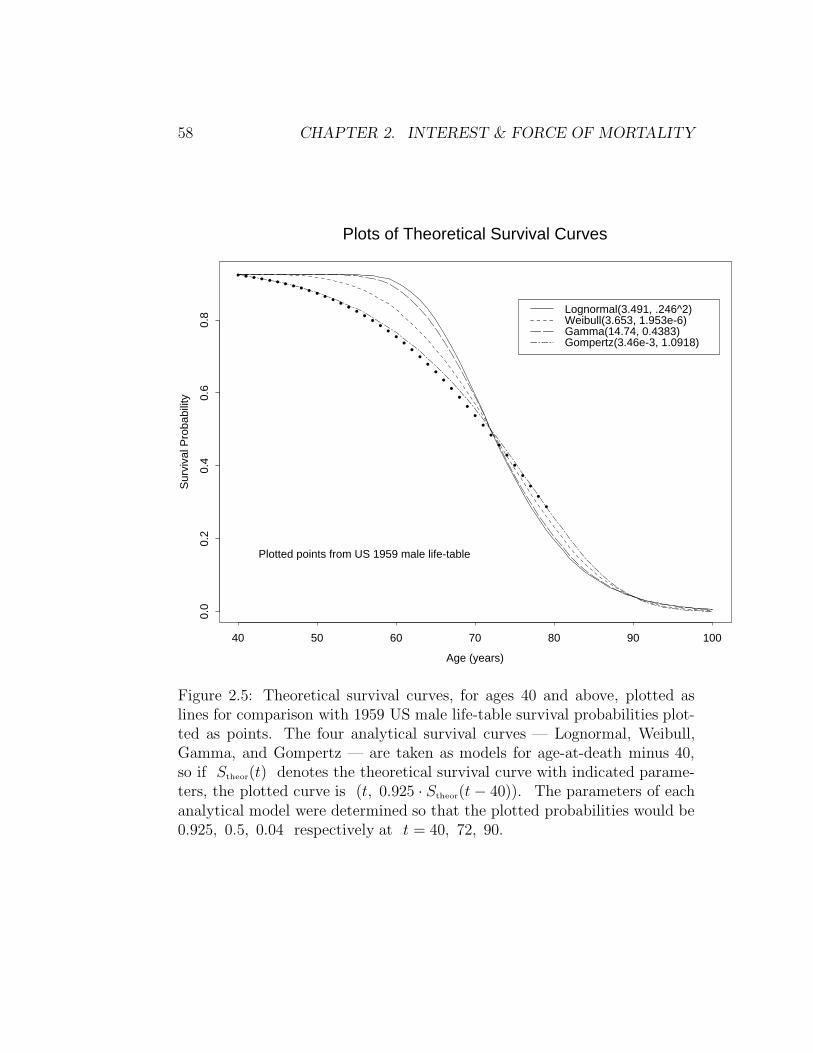
58 CHAPTER 2. INTEREST & FORCE OF MORTALITY
Plots of Theoretical Survival Curves
Age (years)
Sur
viva
l Pro
babi
lity
40 50 60 70 80 90 100
0.0
0.2
0.4
0.6
0.8
• • • • • • • • • • • • • • • • • • • • • ••
••
••
••
••
••
••
••
••
•
Plotted points from US 1959 male life-table
Lognormal(3.491, .246^2)Weibull(3.653, 1.953e-6)Gamma(14.74, 0.4383)Gompertz(3.46e-3, 1.0918)
Figure 2.5: Theoretical survival curves, for ages 40 and above, plotted aslines for comparison with 1959 US male life-table survival probabilities plot-ted as points. The four analytical survival curves — Lognormal, Weibull,Gamma, and Gompertz — are taken as models for age-at-death minus 40,so if Stheor(t) denotes the theoretical survival curve with indicated parame-ters, the plotted curve is (t, 0.925 · Stheor(t − 40)). The parameters of eachanalytical model were determined so that the plotted probabilities would be0.925, 0.5, 0.04 respectively at t = 40, 72, 90.

2.2. FORCE OF MORTALITY & ANALYTICAL MODELS 59
This remark is of especial interest in biostatistics and epidemiology whenthe factor κ is allowed to depend (e.g., by a regression model ln(κ) = β ·Z )on other measured variables (covariates) Z. This model is called the (Cox)Proportional-Hazards model and is treated at length in books on survival dataanalysis (Cox and Oakes 1984, Kalbfleisch and Prentice 1980) or biostatistics(Lee 1992).
Example. Consider a setting in which there are four subpopulations of thegeneral population, categorized by the four combinations of values of twobinary covariates Z1, Z2 = 0, 1. Suppose that these four combinations haverespective conditional probabilities for lives aged x (or relative frequencies inthe general population aged x)
Px(Z1 = Z2 = 0) = 0.15 , Px(Z1 = 0, Z2 = 1) = 0.2
Px(Z1 = 1, Z2 = 0) = 0.3 , Px(Z1 = Z2 = 1) = 0.35
and that for a life aged x and all t > 0,
Pr(T ≥ x + t |T ≥ x, Z1 = z1, Z2 = z2) = exp(−2.5 e0.7z1−.8z2 t2/20000)
It can be seen from the conditional survival function just displayed that theforces of mortality at ages greater than x are
µ(x + t) = (2.5 e0.7z1−.8z2) t/10000
so that the force of mortality at all ages is multiplied by e0.7 = 2.0138 forindividuals with Z1 = 1 versus those with Z1 = 0, and is multiplied bye−0.8 = 0.4493 for those with Z2 = 1 versus those with Z2 = 0. The effecton age-specific death-rates is approximately the same. Direct calculationshows for example that the ratio of age-specific death rate at age x+20 forindividuals in the group with (Z1 = 1, Z2 = 0) versus those in the group with(Z1 = 0, Z2 = 0) is not precisely e0.7 = 2.014, but rather
1 − exp(−2.5e0.7((212 − 202)/20000)
1 − exp(−2.5((212 − 202)/20000)= 2.0085
Various calculations, related to the fractions of the surviving population atvarious ages in each of the four population subgroups, can be performedeasily . For example, to find
Pr(Z1 = 0, Z2 = 1 |T ≥ x + 30)

60 CHAPTER 2. INTEREST & FORCE OF MORTALITY
we proceed in several steps (which correspond to an application of Bayes’rule, viz. Hogg and Tanis 1997, sec. 2.5, or Devore 2007):
Pr(T ≥ x+30, Z1 = 0Z2 = 1|T ≥ x) = 0.2 exp(−2.5e−0.8 302
20000) = 0.1901
and similarly
Pr(T ≥ x + 30 |T ≥ x) = 0.15 exp(−2.5(302/20000)) + 0.1901 +
+ 0.3 exp(−2.5 ∗ e0.7 302
20000) + 0.35 exp(−2.5e0.7−0.8 302
20000) = 0.8795
Thus, by definition of conditional probabilities (restricted to the cohort oflives aged x), taking ratios of the last two displayed quantities yields
Pr(Z1 = 0, Z2 = 1 |T ≥ x + 30) =0.1901
0.8795= 0.2162
2
In biostatistics and epidemiology, the measured variables Z = (Z1, . . . , Zp)recorded for each individual in a survival study might be: indicator of a spe-cific disease or diagnostic condition (e.g., diabetes, high blood pressure, spe-cific electrocardiogram anomaly), quantitative measurement of a risk-factor(dietary cholesterol, percent caloric intake from fat, relative weight-to-heightindex, or exposure to a toxic chemical), or indicator of type of treatment orintervention. In these fields, the objective of such detailed models of covari-ate effects on survival can be: to correct for incidental individual differencesin assessing the effectiveness of a treatment; to create a prognostic index foruse in diagnosis and choice of treatment; or to ascertain the possible risks andbenefits for health and survival from various sorts of life-style interventions.The multiplicative effects of various risk-factors on age-specific death ratesare often highlighted in the news media.
In an insurance setting, categorical variables for risky life-styles, occupa-tions, or exposures might be used in risk-rating, i.e., in individualizing insur-ance premiums. While risk-rating is used routinely in casualty and propertyinsurance underwriting, for example by increasing premiums in response torecent claims or by taking location into account, it can be politically sensi-tive in a life-insurance and pension context. In particular, while differences

2.3. EXERCISE SET 2 61
in mortality by gender and to some extgent by family health history canbe used in calculating insurance and annuity premiums, as can certain life-style factors like smoking, it is currently illegal to use racial differences anddifferences based on genetic testing in this way.
All life insurers must be conscious of the extent to which their policyhold-ers as a group differ from the general population with respect to mortality.Insurers can collect special mortality tables on special groups, such as em-ployee groups or voluntary organizations, and regression-type models like theCox proportional-hazards model may be useful in quantifying group mortal-ity differences when the special-group mortality tables are not based uponlarge enough cohorts for long enough times to be fully reliable. See Chapter6, Section 4, for discussion about the modification of insurance premiums forselect groups.
2.3 Exercise Set 2
(1). The sum of the present value of $1 paid at the end of n years and$1 paid at the end of 2n years is $1. Find (1+ r)2n, where r = annualinterest rate, compounded annually.
(2). Suppose that an individual aged 20 has random lifetime Z withcontinuous density function
f(t) =1
360
(1 +
t
10
), for 20 ≤ t ≤ 80
and 0 for other values of t. (The random variable Z in this problem is aparticular type of age-at-death variable T conditioned on being ≥ 20.)
(a) If this individual has a contract with your company that you mustpay his heirs 106 · (1.4−Z/50) dollars at the exact date of his death if thisoccurs between ages 20 and 70, then what is the expected payment ?
(b) If the value of the death-payment described in (a) should properly bediscounted by the factor exp(−0.08 · (Z − 20)), i.e. by the nominal interestrate of e0.08 − 1 per year) to calculate the present value of the payment,then what is the expected present value of the payment under the insurancecontract ?

62 CHAPTER 2. INTEREST & FORCE OF MORTALITY
(3). Suppose that a continuous random variable T has hazard rate function(= force of mortality)
h(t) = 10−3 ·[7.0 − 0.5t + 2et/20
], t > 0
This is a legitimate hazard rate of Gompertz-Makeham type since its mini-mum, which occurs at t = 20 ln(5), is (17−10 ln(5)) ·10−4 = 9.1 ·10−5 > 0.
(a) Construct a cohort life-table with h(t) as “force of mortality”,based on integer ages up to 70 and cohort-size (= radix ) l0 = 105. (Giveselected numerical entries, preferably calculated by means of a little computerprogram. If you do the arithmetic using hand-calculators and/or tables, giveonly the values for ages which are multiples of 10.)
(b) Find the probability that the random variable T exceeds 30, giventhat it exceeds 3. Hint: find a closed-form formula for S(t) = P (T ≥ t).
(4). Do the Mortgage-Refinancing exercise given as Exercise 2.B in theIllustration on mortgage refinancing at the end of Section 2.1.
(5). (a) The mortality pattern of a certain population may be described asfollows: out of every 98 lives born together, one dies annually until thereare no survivors. Find a simple function that can be used as S(x) for thispopulation, and find the probability that a life aged 30 will survive to attainage 35.
(b) Suppose that for x between ages 12 and 40 in a certain population,10% of the lives aged x die before reaching age x+1 . Find a simple functionthat can be used as S(x) for this population, and find the probability thata life aged 30 will survive to attain age 35.
(6). Suppose that a survival distribution (i.e., survival function based ona cohort life table) has the property that 1px = γ · (γ2)x for some fixed γbetween 0 and 1, for every real ≥ 0. What does this imply about S(x) ?(Give as much information about S as you can.)
(7). If the instantaneous interest rate is r(t) = 0.01 · t for 0 ≤ t ≤ 3,then find the equivalent single effective rate of interest for money invested atinterest throughout the interval 0 ≤ t ≤ 3.

2.3. EXERCISE SET 2 63
(8). Find the accumulated value of $100 at the end of 15 years if thenominal interest rate compounded quarterly (i.e., i(4) ) is 8% for the first 5years, if the effective rate of discount is 7% for the second 5 year interval (i.e.the interval ranging from time 5 to 10), and if the nominal rate of discountcompounded semiannually (m = 2) is 6% for the third 5 year interval.
(9). Suppose that you borrow $1000 for 3 years at 6% effective rate, to berepaid in level payments every six months (twice yearly).
(a) Find the level payment amount P .
(b) What is the present value of the payments you will make if you skipthe 2nd and 4th payments ? (You may express your answer in terms of P . )
(10). A survival function has the form S(t) = max(0, c−tc+t
). If a mortalitytable is derived from this survivalfunction with a radix l0 of 100,000 atage 0, and if l35 = 44, 000 :
(i) What is the terminal age of the table ?
(ii) What is the probability of surviving from birth to age 60 ?
(iii) What is the probability of a person at exact age 10 dying betweenexact ages 30 and 45 ?
(11). A separate life table has been constructed for each calendar year ofbirth, Y , beginning with Y = 1950. The mortality functions for thevarious tables are denoted by the appropriate superscript Y . For each Yand for all ages t
µY (t) = A · k(Y ) + B ct , pY +1t = (1 + r) pY
t
where k is a function of Y alone and A, B, r are constants (with r > 0).If k(1950) = 1, then derive a general expression for k(Y ).
(12). A standard mortality table follows Makeham’s Law with force ofmortality
µ(t) = A + B ct at all ages t
A separate, higher-risk mortality table also follows Makeham’s Law with

64 CHAPTER 2. INTEREST & FORCE OF MORTALITY
force of mortality
µ∗(t) = A∗ + B∗ ct at all ages t
with the same constant c. If for all starting ages the probability of surviving6 years according to the higher-risk table is equal to the probability ofsurviving 9 years according to the standard table, then express each of A∗
and B∗ in terms of A, B, c.
(13). A homeowner borrows $100, 000 at effective annual rate 7% froma bank, agreeing to repay by 30 equal yearly payments beginning one yearfrom the time of the loan.
(a) How much is each payment ?
(b) Suppose that after paying the first 3 yearly payments, the homeowner
misses the next two (i.e. pays nothing on the 4th and 5th anniversaries of
the loan). Find the outstanding balance at the 6th anniversary of the loan,figured at 7% ). This is the amount which, if paid as a lump sum at time6, has present value together with the amounts already paid of $100, 000 attime 0.
(14). A deposit of 300 is made into a fund at time t = 0. The fund paysinterest for the first three years at a nominal monthly rate d(12) of discount.From t = 3 to t = 7, interest is credited according to the force of interestδt = 1/(3t + 3). As of time t = 7, the accumulated value of the fund is574. Calculate d(12).
(15). Calculate the price at which you would sell a $10, 000 30-year couponbond with nominal 6% semi-annual coupon (n = 30, m − 2, i(m) = 0.06),15 years after issue, if for the next 15 years, the effective interest rate forvaluation is ieff = 0.07.
(16). A 6% ‘zero-coupon’ 30-year bond was issued exactly 15 years ago fora face amount of $10, 000. This bond contractually entitles the bearer toreceive 30 years after the issue date the amount accumulated at i = ieff =0.06 on the face amount. Calculate the fair price at which you would sellthis zero-coupon bond, if for the next 15 years, the effective interest rate willbe i′
eff= 0.07.

2.4. WORKED EXAMPLES 65
(17). Suppose that the borrower of a $100, 000 30-year loan with half-yearly payments (m = 2) start in six months from the time of borrowing, andwith nominal interest rate i(2) = .04, has made all payments except for twothat he skipped, the 23’rd and 56’th payments. What lump-sum paymentdid the borrower have to make at the end of 30 years, in addition to his finalpayment, in order to pay off the loan completely ?
(18). In Problem (17), the missed payments did not result in any additionalfees or charges, only in continuing accrued interest on the amounts of themissed payments. Suppose that the missed payments in (17) actually resultin late fees of $200 each of which is added to the balance at the time(s)of missed payments. Now answer the same question as in (17) about theamount of the final lump-sum payment required.
(19). One of the curves plotted in the first part of Figure 2.3 is thelognormal(m,σ2) hazard intensity where σ = 1.3 is fixed and where mwas determined from it by the requirement that the expectation of survivaltime was 75 years. Now find the value m associated with σ = 1.3 if themedian survival time is fixed at 72 years, and find the force of mortality forthis lognormal at 65 years.
(20). A small city issues a bond for twenty million dollars for ten yearsat 5% nominal half-yearly interest (m = 2) and creates a sinking fund intowhich it will make twice-yearly deposits (m′ = 2), from its tax revenue.
(a) Find the amount of the level payment the city must make into thesinking fund if the interest it earns on that fund is 5%, and find the reserve,or accumulated balance, in the sinking fund after 6 years.
(b) Answer the same questions if the city knows it can earn 6% on themoney it deposits into its sinking fund.
2.4 Worked Examples
Example 1. How large must a half-yearly payment be in order that the streamof payments starting immediately be equivalent (in present value terms) at6% interest to a lump-sum payment of $5000, if the payment-stream is tolast (a) 10 years, (b) 20 years, or (c) forever ?

66 CHAPTER 2. INTEREST & FORCE OF MORTALITY
If the payment size is P , then the balance equation is
5000 = 2P · a(2)n = 2P (1 − 1.06−n)/d(2)
Since d(2) = 2(1 − 1/√
1.06) = 2 · 0.02871, the result is
P = (5000 · 0.02871)/(1 − 1.06−n) = 143.57/(1 − 1.06−n)
So the answer to part (c), in which n = ∞, is $143.57. For parts (a) and(b), respectively with n = 10 and 20, the answers are $325.11, $208.62.
Example 2. Assume m is divisible by 2. Express in two differ-ent ways the present value of the perpetuity of payments 1/m at times1/m, 3/m, 5/m, . . . , and use either one to give a simple formula.
This example illustrates the general methods enunciated at the beginningof Section 2.1. Observe first of all that the specified payment-stream isexactly the same as a stream of payments of 1/m at times 0, 2/m, 4/m, . . .forever, deferred by a time 1/m. Since this payment-stream starting at 0
is exactly one-half that of the stream whose present value is a(m/2)∞ , a first
present value expression is
v1/m (1/2) a(m/2)∞
A second way of looking at the payment-stream at odd multiples of 1/mis as the perpetuity-due payment stream ( 1/m at times k/m for allk ≥ 0) minus the payment-stream discussed above of amounts 1/m attimes 2k/m for all nonnegative integers k. Thus the present value has thesecond expression
a(m)∞ − (1/2) a
(m/2)∞
Equating the two expressions allows us to conclude that
(1/2) a(m/2)∞ = a
(m)∞
/(1 + v1/m)
Substituting this into the first of the displayed present-value expressions, andusing the simple expression 1/d(m) for the present value of the perpetuity-due, shows that that the present value requested in the Example is
1
d(m)· v1/m
1 + v1/m=
1
d(m) (v−1/m + 1)=
1
d(m) (2 + i(m)/m)
and this answer is valid whether or not m is even.

2.4. WORKED EXAMPLES 67
Example 3. Suppose that you are negotiating a car-loan of $10, 000. Wouldyou rather have an interest rate of 4% for 4 years, 3% for 3 years, 2% for2 years, or a cash discount of $500 ? Show how the answer depends uponthe interest rate with respect to which you calculate present values, and givenumerical answers for present values calculated at 6% and 8%. Assume thatall loans have monthly payments paid at the beginning of the month (e.g., the4 year loan has 48 monthly payments paid at time 0 and at the ends of 47succeeding months).
The monthly payments for an n-year loan at interest-rate i is 10000/
(12 a(12)n ) = (10000/12) d(12)/(1 − (1 + i)−n). Therefore, the present value
at interest-rate r of the n-year monthly payment-stream is
10000 · 1 − (1 + i)−1/12
1 − (1 + r)−1/12· 1 − (1 + r)−n
1 − (1 + i)−n
Using interest-rate r = 0.06, the present values are calculated as follows:
For 4-year 4% loan: $9645.77
For 3-year 3% loan: $9599.02
For 2-year 2% loan: $9642.89
so that the most attractive option is the cash discount (which would makethe present value of the debt owed to be $9500). Next, using interest-rater = 0.08, the present values of the various options are:
For 4-year 4% loan: $9314.72
For 3-year 3% loan: $9349.73
For 2-year 2% loan: $9475.68
so that the most attractive option in this case is the 4-year loan. (The cashdiscount is now the least attractive option.)
Example 4. Suppose that the force of mortality µ(y) is specified for exactages y ranging from 5 to 55 as
µ(y) = 10−4 · (20 − 0.5|30 − y|)
Then find analytical expressions for the survival probabilities S(y) for exact

68 CHAPTER 2. INTEREST & FORCE OF MORTALITY
ages y in the same range, and for the (one-year) death-rates qx for integerages x = 5, . . . , 54, assuming that S(5) = 0.97.
The key formulas connecting force of mortality and survival function arehere applied separately on the age-intervals [5, 30] and [30, 55], as follows.First for 5 ≤ y ≤ 30,
S(y) = S(5) exp(−∫ y
5
µ(z) dz) = 0.97 exp(−10−4(5(y−5)+0.25(y2−25))
)
so that S(30) = 0.97 e−0.034375 = 0.93722, and for 30 ≤ y ≤ 55
S(y) = S(30) exp(− 10−4
∫ y
30
(20 + 0.5(30 − z)) dz)
= 0.9372 exp(− .002(y − 30) + 2.5 · 10−5(y − 30)2
)
The death-rates qx therefore have two different analytical forms: first, inthe case x = 5, . . . , 29,
qx = S(x + 1)/S(x) = exp(− 5 · 10−5 (10.5 + x)
)
and second, in the case x = 30, . . . , 54,
qx = exp(− .002 + 2.5 · 10−5(2(x − 30) + 1)
)

2.5. USEFUL FORMULAS FROM CHAPTER 2 69
2.5 Useful Formulas from Chapter 2
v = 1/(1 + i)
p. 34
a(m)n =
1 − vn
i(m), a
(m)n =
1 − vn
d(m)
pp. 35–35
a(m)n = v1/m a
(m)n
p. 35
a(∞)n = a
(∞)n = an =
1 − vn
δ
p. 35
a(m)∞ =
1
i(m), a
(m)∞ =
1
d(m)
p. 36
(I(m)a)(m)n = a
(m)∞
(a
(m)n − n vn
)
p. 38
(D(m)a)(m)n = (n +
1
m) a
(m)n − (I(m)a)
(m)n
p. 38
n-yr m’thly Mortgage Paymt :Loan Amt
ma(m)n

70 CHAPTER 2. INTEREST & FORCE OF MORTALITY
p. 39
n-yr Mortgage Bal. amtk
m+ : Bn,k/m =
1 − vn−k/m
1 − vn
p. 42
tpy =S(y + t)
S(y)= exp
(−∫ t
0
µ(y + s) ds
)
p. 48
tqy = 1 − tpy
p. 48
qx = 1qx =dx
lx, px = 1px = 1 − qx
p. 48
µ(y + t) =f(y + t)
S(y + t)= − ∂
∂tlnS(y + t)
p. 49
S(y) = exp(−∫ y
0
µ(t) dt)
p. 52
Unif. Failure Dist.: S(t) =ω − t
ω, f(t) =
1
ω, 0 ≤ t ≤ ω
p. 52
Expon. Dist.: S(t) = e−µt , f(t) = µe−µt , µ(t) = µ , t > 0
p. 52

2.5. USEFUL FORMULAS FROM CHAPTER 2 71
Weibull. Dist.: S(t) = e−λtγ , µ(t) = λγtγ−1 , t > 0
p. 52
Makeham: µ(t) = A + Bct , t ≥ 0
Gompertz: µ(t) = Bct , t ≥ 0
S(t) = exp
(−At− B
ln c(ct − 1)
)
p. 54

72 CHAPTER 2. INTEREST & FORCE OF MORTALITY

Chapter 3
More Probability Theory forLife Tables
This Chapter introduces several key ideas in Probability Theory which areessential for an understanding of the book’s core actuarial topics in Chapter4 and 5. The first of these ideas is that survival from one year to the next canbe regarded for each member of a population as a coin-toss experiment, withsurvival probability px for a life aged x, independently of all other membersof the population. This point of view also provides a convenient vehicle forconducting computer simulations of population survival experience for largeor small life-table populations. Since the life-table summarizes outcomeson a large number of coin-toss experiments, we study next through limittheorems (law of large numbers and central limit theorem) the high degree ofpredictability of these outcomes at the population level. This predictabilitywill be used in later chapters to justify consideration of expected presentvalues of contractual payouts to describe an insurer’s liability, so we preparethe ground by presenting background theory and rules of manipulation forexpectations of discrete-valued random variables. Finally, we complete ourprobability background with further material on interpreting, approximatingand calculating with probabilities and expectations using theoretical modelsof survival between successive years of age.
73

74 CHAPTER 3. PROBABILITY & LIFE TABLES
3.1 Binomial Variables and Limit Theorems
This Section develops basic machinery for the theory of random variableswhich count numbers of successes in large numbers of independent biasedcoin-tosses. The motivation is that in large life-table populations, the numberlx+t who survive t time-units after age x can be regarded as the numberof successes or heads in a large number lx of independent coin-toss trialscorresponding to the further survival of each of the lx lives aged x , which foreach such life has probability tpx. The one preliminary mathematical resultthat the student is assumed to know is the Binomial Theorem stating that(for positive integers N and arbitrary real numbers x, y, z),
(1 + x)N =N∑
k=0
(N
k
)xk , (y + z)N =
N∑
k=0
(N
k
)yk zN−k
Recall that the first of these assertions follows by equating the kth deriv-iatives of both sides at x = 0, where k = 0, . . . , N . The second assertionfollows immediately, in the nontrivial case when z 6= 0, by applying the firstassertion with x = y/z and multiplying both sides by zN . This Theo-rem also has a direct combinatorial consequence. Consider the two-variablepolynomial
(y + z)N = (y + z) · (y + z) · · · (y + z) N factors
expanded by making all of the different choices of y or z from each ofthe N factors (y + z), multiplying each combination of choices out toget a monomial yj zN−j, and adding all of the monomials together. Eachcombined choice of y or z from the N factors (y+ z) can be representedas a sequence (a1, . . . , an) ∈ 0, 1N , where ai = 1 would mean that y
is chosen and ai = 0 would mean that z is chosen in the ith factor. Nowthis combinatorial fact is immediately deduced from the Binomial Theorem:since the coefficient
(Nk
)is the total number of monomial terms yk zN−k
which are collected when (y+z)N is expanded as described, and since thesemonomial terms arise only from the combinations (a1, . . . , aN) of y, zchoices in which precisely k of the values aj are 1’s and the rest are 0’s,
The number of symbol-sequences (a1, . . . , aN) ∈ 0, 1N suchthat
∑Nj=1 aj = k is given, for each k = 0, 1, . . . , N , by

3.1. BINOMIAL VARIABLES & LAW OF LARGE NUMBERS 75
(Nk
)= N(N − 1) · · · (N − k + 1)/ k! . This number
(Nk
), spoken
as ‘N choose k’, therefore counts all of the ways of choosing kelement subsets (the positions j from 1 to N where 1’s occur)out of N objects.
The random experiment of interest in this Section consists of a numberN of independent tosses of a coin, with probability p of coming up headseach time. Such coin-tossing experiments — independently replicated two-outcome experiments with probability p of one of the outcomes, designated‘success’ — are called Bernoulli(p) trials. The space of possible heads-and-tails configurations, or sample space for this experiment, consists of thestrings of N zeroes and ones, with each string a = (a1, . . . , aN) ∈ 0, 1N
being assigned probability pa (1 − p)N−a, where a ≡∑N
j=1 aj. Becauseof the finite additivity axiom of probabilities (saying that Pr(A ∪ B) =Pr(A) + Pr(B) for disjoint events A,B), the rule by which probabilitiesare assigned to sets or events A of more than one string a ∈ 0, 1N isto add the probabilities of all individual strings a ∈ A. We are particularlyinterested in the event (denoted [X = k]) that precisely k of the coin-tosses are heads, i.e., in the subset [X = k] ⊂ 0, 1N consisting of allstrings a such that
∑Nj=1 aj = k. Since each such string has the same
probability pk (1 − p)N−k, and since, according to the discussion followingthe Binomial Theorem above, there are
(Nk
)such strings, the probability
which is necessarily assigned to the event of k successes is
Pr( k successes in N Bernoulli(p) trials ) = P (X = k) =
(N
k
)pk (1−p)N−k
By virtue of this result, the random variable X equal to the number of suc-cesses in N Bernoulli(p) trials, is said to have the Binomial distributionwith probability mass function pX(k) =
(Nk
)pk (1 − p)N−k.
With the notion of Bernoulli trials and the binomial distribution in hand,we now begin to regard the ideal probabilities S(x + t)/S(x) as true butunobservable probabilities tpx = p with which each of the lx lives aged xwill survive to age x + t . Since the mechanisms which cause those livesto survive or die can ordinarily be assumed to be acting independently in aprobabilistic sense, we can regard the number lx+t of lives surviving to the(possibly fractional) age x+t as a Binomial random variable with parametersN = lx, p = tpx. From this point of view, if derived from an actual cohort

76 CHAPTER 3. PROBABILITY & LIFE TABLES
dataset of size equal to the radix , the observed life-table counts lx wouldbe treated as random data which reflect but do not define the underlyingprobabilities xp0 = S(x) of survival to age x. However, common senseand experience suggest that, when l0 is large, and therefore the other life-counts lx for moderate values x are also large, the observed ratios lx+t/lxshould reliably be very close to the ‘true’ probability tpx. In other words,the ratio lx+t/lx is a statistical estimator of the unknown constant tpx .The good property, called consistency, of this estimator to be close with verylarge probability (based upon large life-table size) to the heads-probability itestimates, is established in the famous Law of Large Numbers. We stateand prove the result here only in the setting of binomial random variables,sketching in Section 3.3 how it implies a more general result for finite-valueddiscrete random variables. A more precise quantitative inequality concerningbinomial probabilities, a Large Deviation Inequality which is important in itsown right but more difficult, is stated and proved in the Appendix to thisChapter, Section 3.9.
Theorem 3.1 (Coin-toss Law of Large Numbers) Suppose that X isa Binomial(N, p) random variable, denoting the number of successes in NBernoulli(p) trials. Law of Large Numbers. For arbitrarily small fixedδ, ε > 0, not depending upon N , the number N of Bernoulli trials can bechosen so large that
Pr(|X/N − p | ≥ δ
)≤ ε
Proof. Since the event [ |X/N − p| ≥ δ ] = [ |X −Np| ≥ Nδ ] is the unionof the disjoint events [X = k] for |k − Np| ≥ Nδ, which in turn consistof all outcome-strings (a1, . . . , aN) ∈ 0, 1N for which
∑Nj=1 aj = k with
|k −Np| ≥ Nδ, the subset of the binomial probability mass function valuespX (k) with |k − Np| ≥ Nδ are summed to provide
Pr(|X/N−p| ≥ δ) =∑
k: |k−Np|≥Nδ
Pr(X = k) =∑
k: |k−Np|≥Nδ
(N
k
)pk (1−p)N−k
This summation is term-by-term less than or equal to
∑
k: |k−Np|≥Nδ
(N
k
)pk (1−p)N−k (k − Np)2
(Nδ)2≤
N∑
k=0
(N
k
)pk (1−p)N−k (k − Np)2
(Nδ)2
(3.1)

3.1. BINOMIAL VARIABLES & LAW OF LARGE NUMBERS 77
where we have made the second some larger by including more nonnegativeterms in it. However, direct summation shows
N∑
k=0
k
(N
k
)pk (1 − p)N−k =
N∑
k=1
kpN · (N − 1)!
k(k − 1)!(N − k)!pk−1 (1 − p)N−k
which after replacing k − 1 by l, becomes with the aid of the Binomial The-orem
= Np
N−1∑
l=0
(N − 1
l
)pl (1 − p)N−1−l = Np
and similarly (now with j = k − 2)
N∑
k=0
k(k−1)
(N
k
)pk (1−p)N−k =
N∑
k=2
p2 N(N − 1) (N − 2)!
(k − 2)!(N − k)!pk−2 (1−p)N−k
= N(N − 1)p2
N−2∑
j=0
(N − 2
j
)pj (1 − p)N−2−j = N(N − 1) p2
Putting together the last calculations, and simplifying algebraically, it is easyto check via the equality (k −Np)2 = k(k − 1)− (2Np− 1)k +(Np)2, that
N∑
k=0
(k − Np)2
(N
k
)pk (1 − p)N−k = N p(1 − p)
Substituting this final relation into (3.1) now shows that
Pr(|X/N − p| ≥ δ) ≤ Np(1 − p)
(Nδ)2=
p(1 − p)
Nδ2
The assertion of the Theorem now follows by taking N ≥ (p(1−p)/(εδ2). 2
3.1.1 Probability Bounds & Approximations
Theorem 3.1 provides only a very crude upper bound to the probability withwhich |X/N − p| ≥ δ. A much more accurate upper bound in given inTheorem 3.2 of the Appendix to the Chapter (Sec. 3.9). To see why more

78 CHAPTER 3. PROBABILITY & LIFE TABLES
accurate bounds are needed, consider the case where N = 1000, p = 0.1,and δ = 0.03. The exact Binomial(1000, 0.1) probability of (number ofsuccesses in N Bernoulli(p) trials falling in) [0, N(p − δ)]∪ [N(p + δ), N ] =[0, 70] ∪ [130, 1000] is 0.001916, while the upper bound established in theproof of Theorem 3.1 is (.1)(.9)/(1000(.03)2) = 0.1, more than fifty timeslarger ! On the other hand, the upper bound provided by the inequalities ofTheorem 3.2, as in formula (3.30), is 0.0198.
Much closer approximations to the exact probabilities for Binomial(N, p)random variables to fall in intervals around Np are obtained from the Normaldistribution approximation
Pr(a ≤ X ≤ b) ≈ Φ
(b −Np√Np(1 − p)
)− Φ
(a − Np√Np(1 − p)
)(3.2)
where Φ is the standard normal distribution function given explicitly inintegral form in formula (3.29) below. This approximation is the DeMoivre-Laplace Central Limit Theorem (Feller vol. 1, 1957, pp. 168-73), whichsays precisely that the difference between the left- and right-hand sides of(3.2) converges to 0 when p remains fixed, as n → ∞. Moreover, therefined form of the DeMoivre-Laplace Theorem given in the Feller (1957,p. 172) reference says that each of the ratios of probabilities
Pr(X < a)/
Φ( a− Np√
Np(1 − p)
), Pr(X > b)
/[1 −Φ
( b − Np√Np(1 − p)
)]
converges to 1 if the ‘deviation’ ratios (b − Np)/√
Np(1 − p) and
(a − Np)/√
Np(1 − p) are of smaller order than N−1/6 when N getslarge. This result suggests the approximation
Normal approx. = Φ
(Nδ√
Np(1 − p)
)− Φ
(−Nδ√
Np(1 − p)
)(3.3)
for the true binomial probability Pr(|X/N − p| ≤ δ). In the examplediscussed above, with N = 1000, p = 0.1, δ = 0.03, where the exactBinomial(N, p) probability of |X/N −p| ≤ δ was 1− .00192 = .99808, thenormal approximation (3.3) is 0.99843.
To give a feeling for the probabilities with which observed life-table ra-tios reflect the true underlying survival-rates, we have collected in Table 3.1

3.1. BINOMIAL VARIABLES & LAW OF LARGE NUMBERS 79
Table 3.1: Probabilities (in col. 6) with which various Binomial(lx, kpx)random variables lie within a factor 1 ± ε of their expectations, togetherwith lower bounds (in Col. 7) for these probabilities derived from the large-deviation inequalities (3.30)-(3.31). The final column contains the normalapproximations based on (3.3) to the exact probabilities in column 6.
Cohort Age Time Prob. Toler. Pr. within Lower Normaln = lx x k p = kpx ε factor 1 ± ε bound approx.10000 40 3 0.99 .003 .9969 .9760 .997210000 40 5 0.98 .004 .9952 .9600 .994910000 40 10 0.94 .008 .9985 .9866 .99851000 40 10 0.94 .020 .9863 .9120 .9877
10000 70 5 0.75 .020 .9995 .9950 .99951000 70 5 0.75 .050 .9938 .9531 .9938
10000 70 10 0.50 .030 .9973 .9778 .99731000 70 10 0.50 .080 .9886 .9188 .9886
various exact binomial probabilities and their counterparts from the approx-imation of (3.3) and the inequality (3.30) of Section 3.9. The illustrationconcerns cohorts of lives aged x of various sizes lx, together with ‘theo-retical’ probabilities kpx with which these lives will survive for a period ofk = 1, 5, or 10 years. The probability experiment determining the size ofthe surviving cohort lx+k is modelled as the tossing of lx independent coinswith common heads-probability kpx : then the surviving cohort-size lx+k
is viewed as the Binomial(lx, kpx) random variable equal to the number ofheads in those coin-tosses. In Table 3.1 are given various combinations ofx, lx, k, kpx which might realistically arise in an insurance-company life-table, together, with the true and estimated (from Theorem 3.2 and from(3.3)) probabilities with which the ratios lx+k/lx agree with kpx to withina fraction ε of the latter. Columns 6 and 7 in the Table show how likely thelife-table ratios are to be close to the ‘theoretical’ values, but also show thatthe lower bounds, while also often close to 1, are still noticeably smallerthan the actual values.
Although the deviation-ratios in estimating life-table probabilities areoften close to or larger than N−1/6, not smaller as they should be for appli-cability of (3.3), the normal approximations in the final column of Table 3.1

80 CHAPTER 3. PROBABILITY & LIFE TABLES
below are sensationally close to the correct binomial probabilities in column6. A still more refined theorem which justifies this is given by Feller (1972,section XVI.7 leading up to formula 7.28, p. 553).
3.2 Simulation of Discrete Lifetimes
We began by regarding life-table ratios lx/l0 in large cohort life-tables asdefining integer-age survival probabilities S(x) = xp0. We said that if thelife-table was representative of a larger population of prospective insureds,then we could imagine a newly presented life aged x as being randomlychosen from the life-table cohort itself. We motivated the conditional prob-ability ratios in this way, and similarly expectations of functions of life-tabledeath-times were averages over the entire cohort. Although we found thecalculus-based formulas for life-table conditional probabilities and expec-tations to be useful, at that stage they were only ideal approximations ofthe more detailed but still exact life-table ratios and sums. At the nextstage of sophistication, we began to describe the (conditional) probabilities
tpx ≡ S(x+ t)/S(x) based upon a smooth survival function S(x) as a truebut unknown survival distribution, hypothesized to be of one of a numberof possible theoretical forms, governing each member of the life-table cohortand of further prospective insureds. Finally, the life-table can also be viewedas in Appendix A as an idealized set of data, with each ratio lx+t/lx equal tothe relative frequency of success among a set of lx imagined Bernoulli(tpx)trials which Nature performs upon the cohort of lives aged x . With themathematical justification of the Law of Large Numbers, we come full circle:these relative frequencies are random variables, but they are not very ran-dom. That is, if the size lx of the cohort of surviving lives aged x is large,the later fractions lx+t/lx of survivors at x+ t to those at x are extremelylikely to lie within a very small tolerance of tpx. The Law of Large Num-bers applies equally when the age-x survivors have been sampled by somemore complicated method than simply watching a cohort from birth. Thus,in the realistic data-collection scenarios discussed in Appendix A, where thesizes lx of lives under observation at age x are large but the probabilitiespx are unknown, the life-table ratios lx+1/lx are highly accurate statisticalestimators of the life-table probabilities .

3.2. SIMULATION OF DISCRETE LIFETIMES 81
Table 3.2: Illustrative Real and Simulated Life-Table Data
Age x lx in 1959-61 Life-Table Simulated l∗x9 96801 9675319 96051 9598929 94542 9442839 92705 9257649 88178 8790159 77083 7679369 56384 5618679 28814 28657
To make this discussion more concrete, we illustrate the difference be-tween the entries in a life-table and the entries one would observe as datain a randomly generated life-table of the same size using the initial life-tableratios as exact survival probabilities. We used as a source of life-table countsthe Mortality Table for U.S. White Males 1959-61 reproduced as Table 2 onpage 11 of C. W. Jordan’s (1967) book on Life Contingencies. That is, usingthis Table with radix l0 = 105 , with counts lx given for integer ages x from1 through 80, we treated the probabilities px = lx+1/lx for x = 0, . . . , 79 asthe correct one-year survival probabilities for a second, computer-simulatedcohort life-table with radix l∗0 = 105. Using simulated random variablesgenerated in R, we successively generated, as x runs from 1 to 79, randomvariables l∗x+1 ∼ Binomial (l∗x, px). In other words, the mechanism of sim-ulation of the sequence l∗0, . . . , l
∗79 was to make the variable l∗x+1 depend
on previously generated l∗1, . . . , l∗x only through l∗x, and then to generate
l∗x+1 as though it counted the heads in l∗x independent coin-tosses withheads-probability px. A comparison of the actual and simulated life-tablecounts for ages 9 to 79 in 10-year intervals, is given below. The completesimulated life-table was given earlier as Table 1.1.
The implication of Table 3.2 is unsurprising: with radix as high as 105,the agreement between the initial and randomly generated life-table countsis extremely good. The Law of Large Numbers guarantees good agreement,with very high probability, between the ratios lx+10/lx (which here playthe role of the probability 10px of success in l∗x Bernoulli trials) and thecorresponding simulated random relative frequencies of success l∗x+10/l
∗x. For
example, with x = 69, the final simulated count of l∗79 = 28657 lives

82 CHAPTER 3. PROBABILITY & LIFE TABLES
aged 79 is the success-count in l∗69 = 56186 Bernoulli trials with success-probability 28814/56384 = .51103. With this success-probability, the nor-mal approximation (3.3) says that the simulated count l∗79 will differ from.51103 · 56186 = 28712.8 by 300 or more in either direction with probabilityapproximately 0.0115. (The exact binomial probabilty of the same event is0.0113.).
The R code used to generate Table 3.2 is very simple. If lvec denotes avector of values (l0, lx(1), lx(2), . . . , lx(K)) of numbers of surviving lives in acohort life-table with radix l0, where the integer ages 0, x(1), x(2), . . . , x(K)are not necessarily evenly spaced, then the statements
K = length(lvec)-1 ; pvec = lvec[2:(K+1)]/lvec[1:K]
create the vector of hypothetical survival probabilities, pvec[j]= lx(j+1)/lxj , j =0, . . . ,K − 1, and here is a small function to generate the (K + 1)-vectortt lstar consisting of l∗0 ≡ l0 together with the output simulated valuesl∗x(1), . . . , lx(K) :
LifTabSim = function(lvec)
K = length(lvec)-1
lstar = c(lvec[1],rep(0,K))
for (j in 1:K) lstar[j+1] =
rbinom(1,lstar[j],lvec[j+1]/lvec[j])
lstar
The syntax to generate a vector like the third column of Table 3.2 from thesecond, where lvec consists of the radix l0 = 105 concatenated with column2, is: LifTab(lvec)[2:9]. As a further example of such a simulation,suppose that 1000 individuals aged 40 have successive probabilities 10px =0.85, 0.77, 0.70, 0.65, 0.4 for x = 40, 50, 60, 70, 80, then we can simulatetwice, independently and output in R the numbers of surviving lives at theseages, as follows:
pvec = c(0.85, 0.77, 0.70, 0.65, 0.4)
Lvec = 1000*cumprod(c(1,pvec))
matrix(c(seq(40,80,10), pvec, LifTabSim(Lvec)[2:6],
LifTabSim(Lvec)[2:6]), nrow=4, ncol=5, byrow=T,

3.2. SIMULATION OF DISCRETE LIFETIMES 83
dimnames=list(c("Ages","10_p_x","Sim#1 l_x",
"Sim#2 l_x"), NULL))
[,1] [,2] [,3] [,4] [,5]
Ages 40.00 50.00 60.0 70.00 80.0
10_p_x 0.85 0.77 0.7 0.65 0.4
Sim#1 l_x 842.00 638.00 450.0 296.00 133.0
Sim#2 l_x 854.00 662.00 483.0 344.00 129.0
From small experiments like this, we can see that the variability in the sim-ulated numbers l∗x is considerable for l0 of 1000 or less.
Exercise 3.A. With the same probabilities 10px use R to simulate 10 timesindependently the numbers of survivors at ages 40, 50, . . . , 80.
(a). What is the spread between the smallest and largest number surviv-ing at each age across your 10 simulations ?
(b). Regarding your 10 sets of simulated numbers of survivors as indepen-dent datasets, if the underlying life-table probabilities were unknown, whatwould be your best estimate of the probability 20p40 ?
(c). Combining the 10 simulated datasets you generated in (b), what isyour best estimate of the probability 20p40 ?

84 CHAPTER 3. PROBABILITY & LIFE TABLES
3.3 Expectation of Discrete Random Variables
The Binomial random variables discussed in this Chapter are examples ofso-called discrete random variables, that is, random variables Z with adiscrete (usually finite) list of possible outcomes z, with a corresponding listof probabilities or probability mass function values pZ(z) with which each ofthose possible outcomes occur. These probabilities pZ(z) must be positivenumbers which summed over all possible values z add to 1. In an insur-ance context, think for example of Z as the unforeseeable future damage orliability upon the basis of which an insurer has to pay some scheduled claimamount c(Z) to fulfill a specific property or liability insurance policy. TheLaw of Large Numbers says that we can have a frequentist operational inter-pretation of each of the probabilities pZ(z) with which a claim of size c(z)is presented. In a large population of N independent policyholders, eachgoverned by the same probabilities pZ(·) of liability occurrences, for eachfixed damage-amount z we can imagine a series of N Bernoulli(pZ (z))trials, in which the jth policyholder is said to result in a ‘success’ if hesustains a damage amount equal to z , and to result in a ‘failure’ otherwise.The Law of Large Numbers (Theorem 3.7) for these Bernoulli trials says thatthe number out of these N policyholders who do sustain damage z is forlarge N extremely likely to differ by no more than δN from N pZ(z).
Returning to a general discussion, suppose that Z is a discrete randomvariable with a finite list of possible values z1, . . . , zm, and let c(·) be areal-valued (nonrandom) cost function such that c(Z) represents an eco-nomically meaningful cost incurred when the random variable value Z isgiven. Suppose that a large number N of independent individuals give riseto respective values Zj, j = 1, . . . , N and costs c(Z1), . . . , c(ZN ). Here in-dependent means that the mechanism causing different individual Zj valuesis such that information about the values Z1, . . . , Zj−1 does not change the(conditional) probabilities with which Zj takes on its values, so that for allj, i, and b1, . . . , bj−1,
P (Zj = zi |Z1 = b1, . . . , Zj−1 = bj−1 ) = pZ(zi)
Then the Law of Large Numbers, applied as above, says that out of thelarge number N of individuals it is extremely likely that approximatelypZ(k) · N will have their Z variable values equal to k, where k rangesover z1, . . . , zm. It follows that the average costs c(Zj) over the N

3.3. EXPECTATION OF DISCRETE RANDOM VARIABLES 85
independent individuals — which can be expressed exactly as
N−1
N∑
j=1
c(Zj) = N−1
m∑
i=1
c(zi) · #j = 1, . . . , N : Zj = zi
— is approximately given by
N−1
m∑
i=1
c(zi) · (N pZ(zi)) =m∑
i=1
c(zi) pZ(zi)
In other words, the Law of Large Numbers implies that the average costper trial among the N independent trials resulting in random variablevalues Zj and corresponding costs c(Zj) has a well-defined approximate(actually, a limiting) value for very large N
Expectation of cost = E(c(Z)) =m∑
i=1
c(zi) pZ(zi) (3.4)
As an application of the formula for expectation of a discrete randomvariable, consider the expected value of a cost-function g(T ) of a lifetimerandom variable which is assumed to depend on T only through the functiong([T ]) of the integer part of T . This expectation was interpreted earlier asthe average cost over all members of the specified life-table cohort. Now theexpectation can be verified to coincide with the life-table average previouslygiven, if the probabilities S(j) in the following expression are replaced bythe life-table estimators lj/l0. Since P ([T ] = k) = S(k) − S(k + 1), thegeneral expectation formula (3.4) yields
E(g(T )) = E(g([T ]) =ω−1∑
k=0
g(k) (S(k) − S(k + 1)) (3.5)
which, after replacing S(k) − S(k + 1) =∫ k+1
kf(t) dt and [t] = k for
k ≤ t < k + 1, becomes
ω−1∑
k=0
g(k)
∫ k+1
k
f(t) dt =ω−1∑
k=0
∫ k+1
k
g([t]) f(t) dt =
∫ ω
0
g([t]) f(t) dt
agreeing precisely with formula (1.3). Similarly, evaluating the discrete con-ditional expectation given T ≥ x means applying the formula (3.4) to the

86 CHAPTER 3. PROBABILITY & LIFE TABLES
function c(Z) = g(Z) of the discrete random variable Z = [T ] usingthe conditional probability mass function P (Z = k) = P ([T ] = k |T ≥x) = (S(k) − S(k + 1))/S(x) for all integers k ≥ x (and with probability0 assigned to all integers k < x.) Then the conditional expectation is
E(g([T ]) |T ≥ x) =ω−1∑
k=x
S(k) − S(k + 1)
S(x)g(k) =
ω−1∑
k=x
g(k)
S(x)
∫ k+1
k
f(t) dt
or
E(g([T ] |T ≥ x) =
ω−1∑
k=x
∫ k+1
k
g([t])
S(x)f(t) dt =
∫ ω
0
g([t])f(t)
S(x) dt
agreeing precisely with formula (1.5).
The preceding discussion shows that expectations or conditional expec-tations of functions of whole-year ages can equivalently be calculated usingthe expectation formulas for discrete or continuous random variables. In thediscrete case, however, the expressions require knowledge only of the prob-abilities S(y) of survival for whole-year or integer ages y. Indeed, in thepreceding (discrete-version) formula, for E(g([T ]) |T ≥ x), let k ≥ x bereplaced by k = x + j, and express
S(k) − S(k + 1)
S(x)=
S(x + j)
S(x)
(1 − S(x + j + 1
S(x + j)
)= jpx (1 − px+j)
Then
E(g([T ]) |T ≥ x) =
ω−1∑
k=x
S(k)− S(k + 1)
S(x)g(k) =
ω−x−1∑
j=0
jpx (1−px+j ) g(x+j)
(3.6)
Just as we did in the context of expectations of functions of the life-table waiting-time random variable T , we can interpret the Expectation as aweighted average of values (costs, in this discussion) which can be incurred ineach trial, weighted by the probabilities with which they occur. There is ananalogy in the continuous-variable case, where Z would be a random variablewhose approximate probabilities of falling in tiny intervals [z, z + dz] aregiven by fZ(z)dz, where fZ(z) is a nonnegative density function integratingto 1. In this case, the weighted average of cost-function values c(z) whicharise when Z ∈ [z, z + dz], with approximate probability-weights fZ(z)dz,is written as a limit of sums or an integral, namely
∫c(z) f(z) dz.

3.3. EXPECTATION OF DISCRETE RANDOM VARIABLES 87
3.3.1 Rules for Manipulating Expectations
We have separately defined expectation for continuous and discrete randomvariables. In the continuous case, we treated the expectation of a specifiedfunction g(T ) of a lifetime random variable governed by the survival functionS(x) of a cohort life-table, as the approximate numerical average of the valuesg(Ti) over all individuals i with data represented through observed lifetimeTi in the life-table. The discrete case was handled more conventionally,along the lines of a ‘frequentist’ approach to the mathematical theory ofprobability. First, we observed that our calculations with Binomial(n, p)random variables justified us in saying that the sum X = Xn of a largenumber n of independent coin-toss variables ε1, . . . , , εn, each of which is1 with probability p and 0 otherwise, has a value which with very highprobability differs from n·p by an amount smaller than δn, where δ > 0 isan arbitrarily small number not depending upon n. The Expectation p ofeach of the variables εi is recovered approximately as the numerical averageX/n = n−1
∑ni=1 εi of the independent outcomes εi of independent trials.
This Law of Large Numbers extends to arbitrary sequences of independentand identical finite-valued discrete random variables, saying that
if Z1, Z2, . . . are independent random variables, in the sensethat for all k ≥ 2 and all numbers r,
P (Zk ≤ r |Z1 = z1, . . . , Zk−1 = zk−1 ) = P (Z1 ≤ r)
regardless of the precise values z1, . . . , zk−1, then for each δ > 0,as n gets large
P(|n−1
n∑
i=1
c(Zi) − E(c(Z1))| ≥ δ)
−→ 0 (3.7)
where, in terms of the finite set S of possible values of Z ,
E(c(Z1)) =∑
z∈S
c(z)P (Z1 = z) (3.8)
We do not give any further proof here, but the motivating arguments given,together with straightforward manipulations using the result of Theorem 3.7,

88 CHAPTER 3. PROBABILITY & LIFE TABLES
are an essentially complete proof of (3.7). It is also a fact that the Law ofLarge Numbers given in equation (3.7) continues to hold if the definitionof independent sequences of random variables Zi is suitably generalized, aslong as either
Zi are discrete with infinitely many possible values defining aset S, and the expectation is as given in equation (3.8) abovewhenever the function c(z) is such that
∑
z∈S
|c(z)|P (Z1 = z) < ∞
or
the independent random variables Zi are continuous, all withthe same density f(t) such that P (q ≤ Z1 ≤ r) =
∫ r
qf(t) dt,
and expectation is defined by
E(c(Z1)) =
∫ ∞
−∞c(t) f(t) dt (3.9)
whenever the function c(t) is such that
∫ ∞
−∞|c(t)| f(t) dt < ∞
All of this shows that there really is no choice in devising an appropri-ate definition of expectations of cost-functions defined in terms of randomvariables Z, whether discrete or continuous. For the rest of this book, andmore generally in applications of probability within actuarial science, we areinterested in evaluating expectations of various functions of random variablesrelated to the contingencies and uncertain duration of life. Many of theseexpectations concern superpositions of random amounts to be paid out afterrandom durations. The following rules for the manipulation of expectationsarising in such superpositions considerably simplify the calculations. Assumein what follows that all random payments and times are functions of a singlelifetime random variable T .

3.3. EXPECTATION OF DISCRETE RANDOM VARIABLES 89
(1). If a payment consists of a nonrandom multiple (e.g., face-amountF ) times a random amount c(T ), then the expectation of the payment isthe product of F and the expectation of c(T ):
Discrete case: E(Fc(T )) =∑
t
F c(t)P (T = t)
= F∑
t
c(t)P (T = t) = F · E(c(T ))
Continuous case: E(Fc(T )) =
∫F c(t)f(t) dt = F
∫c(t)f(t) dt = F ·E(c(T ))
(2). If a payment consists of the sum of two separate random paymentsc1(T ), c2(T ) (which may occur at different times, taken into account bytreating both terms ck(T ) as present values as of the same time), then theoverall payment has expectation which is the sum of the expectations of theseparate payments:
Discrete case: E(c1(T ) + c2(T )) =∑
t
(c1(t) + c2(t))P (T = t)
=∑
t
c1(t)P (T = t) +∑
t
c2(t)P (T = t) = E(c1(T )) + E(c2(T ))
Continuous case: E(c1(T ) + c2(T )) =
∫(c1(t) + c2(t)) f(t) dt
=
∫c1(t) f(t) dt +
∫c2(t) f(t) dt = E(c1(T )) + E(c2(T ))
Thus, if an uncertain payment under an insurance-related contract, basedupon a continuous lifetime variable T with density fT , occurs only ifa ≤ T < b and in that case consists of a payment of a fixed amount Foccurring at a fixed time h, then the expected present value under a fixednonrandom interest-rate i with v = (1 + i)−1, becomes by rule (1) above,
E(vh F I[a≤T<b]) = vh F E(I[a≤T<b])
where the indicator-notation I[a≤T<b] denotes a random quantity which is1 when the condition [a ≤ T < b] is satisfied and is 0 otherwise. Since

90 CHAPTER 3. PROBABILITY & LIFE TABLES
an indicator random variable has the two possible outcomes 0, 1 like thecoin-toss variables εi above, we conclude that E(I[a≤T<b]) = P (a ≤ T <
b) =∫ b
afT (t) dt, and the expected present value above is
E(vh F I[a≤T<b]) = vh F
∫ b
a
fT (t) dt
(3). The expectation of a nonnegative-integer-valued random variablecan sometimes be simplified considerably by means of the following usefulLemma.
Lemma 3.1 Let Z be a nonnegative-integer-valued random variable. Then
EZ =∞∑
j=1
P (Z ≥ j) (3.10)
The Lemma is proved using the rule (Fubini-Tonelli theorem for doublesummation) that the order of a double summation of nonnegative summandscan always be reversed:
EZ =
∞∑
k=0
k pZ(k) =
∞∑
k=1
k∑
j=1
pX(k) =
∞∑
j=1
∞∑
k=j
pZ(k) =
∞∑
j=1
P (Z ≥ j)
3.3.2 Curtate Expectation of Life
One example of a function of the number [T ] of whole years of life, whoseconditional expectation is useful and interpretable, is the whole-year residuallife [T ]−x for a life aged x, where x is an integer age. The expectation, nec-essarily conditional on the attained age x, is called curtate mean residuallife or curtate life expectancy,
ex = E( [T ]− x |T ≥ x ) =ω−1∑
t=x
P (t ≤ T < t + 1)
P (T ≥ x)(t− x) (3.11)

3.4. INTERPRETING FORCE OF MORTALITY 91
Substituting the formula (3.6) with g(t) = t − x gives this formula inthe alternative form
ex = E( [T ]− x |T ≥ x ) =ω−x−1∑
j=0
jpx (1 − px+j) j (3.12)
A third useful version of this formula can be found by applying formula(3.10) of Lemma 3.1 to the nonnegative integer valued random variable Z =[T ]− x with probability masses calculated conditionally given T ≥ x. Thisyields
ex = E( [T ]− x |T ≥ x ) =ω−x−1∑
j=1
P ([T ]− x ≥ j |T ≥ x) =ω−x−1∑
j=1
jpx
(3.13)
The extension of these expectation formulas to give mean residual life-times which are not truncated to whole years rests on survival function anddensity formulas which specify mortality rates between birthdays. The fol-lowing two sections are devoted to a deeper study of continuous mortalitymodels and interpolation approximations.
3.4 Interpreting Force of Mortality
This Section consists of remarks, relating the force of mortality for a con-tinuously distributed lifetime random variable T (with continuous densityfunction f ) to conditional probabilities for discrete random variables. In-deed, for m large (e.g. as large as 4 or 12), the discrete random variable[Tm]/m gives a close approximation to T and represents the attained ageat death measured in whole-number multiples of fractions h = one mth
of a year. (Here [·] continues to denote the greatest integer less than orequal to its real argument.) Since surviving an additional time t = nh canbe viewed as successively surviving to reach times h, 2h, 3h, . . . , nh, andsince (by the definition of conditional probability)
P (A1 ∩ · · · ∩ An) = P (A1) · P (A2|A1) · · ·P (An|A1 ∩ · · · ∩ An−1)
we have (with the interpretation Ak = T ≥ x + kh )
nhpx = hpx · hpx+h · hpx+2h · · · hpx+(n−1)h

92 CHAPTER 3. PROBABILITY & LIFE TABLES
The form in which this formula is most often useful is the case h = 1: forintegers k ≥ 2,
kpx = px · px+1 · px+2 · · · px+k−1 (3.14)
Every continuous waiting-time random variable can be approximated bya discrete random variable with possible values which are multiples of afixed small unit h of time, and therefore the random survival time canbe viewed as the (first failure among a) succession of results of a sequenceof independent coin-flips with successive probabilities hpkh of heads. Bythe Mean Value Theorem applied up to second-degree terms on the functionS(x + h) expanded about h = 0,
S(x+h) = S(x) + hS ′(x) +h2
2S ′′(x+τh) = S(x) − hf(x) − h2
2f ′(x+τh)
for some 0 < τ < 1, if f is continuously differentiable. Therefore, usingthe definition of µ(x) as f(x)/S(x) given on page 49,
hpx = 1 − h ·[S(x)− S(x + h)
hS(x)
]= 1 − h
(µ(x) +
h
2
f ′(x + τh)
S(x)
)
Going in the other direction, the previously derived formula
hpx = exp
(−∫ x+h
x
µ(y) dy
)
can be interpreted by considering the fraction of individuals observed to reachage x who thereafter experience hazard of mortality µ(y) dy on successiveinfinitesimal intervals [y, y+dy] within [x, x+h). The lives aged x surviveto age x + h with probability equal to a limiting product of infinitesimalterms (1−µ(y) dy) ∼ exp(−µ(y) dy), yielding an overall conditional survivalprobability equal to the negative exponential of accumulated hazard over[x, x + h).
3.5 Interpolation Between Integer Ages
Cohort life-table data lx and the probability quantities jpx derived fromthem (for integers j) depend on and are determined by the survival func-tion S(k) values only at integer arguments k. Yet many expectations of

3.5. INTERPOLATION BETWEEN INTEGER AGES 93
functions important in actuarial applications necessarily involve the survivalfunction values between integer ages. It is possible to approximate these onlybecause, for all but the very youngest and oldest ages, the survival functionfor human lives is very smooth within years of age, with derivatives that arenot dramatically large and themselves do not change rapidly. In terms ofcalculus concepts, the function value S(x + t) for integer x and 0 ≤ t < 1is given approximately by the Taylor series formula
S(x + t) = S(x) + t S ′(x) +1
2t2 S ′′(x + θt)
= S(x) − t f ′(x) − 1
2t2 f ′(x + θt) (3.15)
where θ ∈ (0, 1) in the argument of S ′′ in the third term (the mean-valuetype remainder) of the first line, and where the second line uses the definitionf(x + t) = −S ′(x + t) valid at all nonnegative integers x and t ∈ [0, 1).
While we will later use Taylor expansions like (3.15) to approximateexpectations E(g(T )) and conditional expectations E(g(T ) |T ≥ x), fornow we focus on understanding what (3.15) says about the approximateprobability distribution of the lifetime variable T within years of age. IfS ′′ = −f ′ is small, as is undoubtedly true for human lifetime between ages2 and 75 in modern public health conditions, then it is tempting to im-pose the direct modelling assumption S(x + t) ≡ S(x) − tf(x) for integerx and t ∈ [0, 1), together with continuity of S at all integer points.This assumption, often called the actuarial approximation, says that for any0 ≤ a < b < 1,
P (T ∈ [x+a, x+b) | [T ] = x) =S(x + a) − S(x + b)
(S(x) − S(x + 1)=
(b − a) f(x)
f(x)= b−a
In other words, the ‘actuarial approximation’ says that failures known tooccur within the year between the x and x+1 birthdays are actually uniformlydistributed (have constant conditional density of 1) within that year.
The ‘actuarial-approximation’ assumption can be understood either aspiecewise linearity, on exact-age intervals [x, x + 1), of the continuous sur-vival function S(y) or equivalently as piecewise constancy of the densityfunction f(y) = −S ′(y). This assumption is by far the most commonlyused one in actuarial work. Two other related possible approximations can

94 CHAPTER 3. PROBABILITY & LIFE TABLES
be obtained by Taylor expanding not S(x+t) itself but rather the functionslog S(x + t) or 1/S(x + t). It turns out that the first of these alternativeassumptions, piecewise linearity of log S(x + t) or equivalently piecewiseconstancy within intervals x, x + 1) of d
dylog S(y) = −f(y)/S(y) ≡ µ(y)
is well known and has historically been widely used by biostatisticians. Manymodels in biostatistics or reliability have been formulated with piecewise con-stant hazards (recall that biostatisticians call µ(y) the hazard function whileactuaries call it force of mortality). The third assumption introduced here,that of piecewise linearity of 1/S(y), is called the Balducci hypothesis,and is studied by actuarial students largely for historical reasons and as asource of examination problems, since it will be seen immediately below for-mula (3.22) to have properties which make it unsuitable as a realistic modelfor survival.
To proceed formally, assume that values S(x) for x = 0, 1, 2, . . . havebeen specified or estimated. Approximations to S(y), f(y) and µ(y)between integers are usually based on one of the following assumptions:
(i) (Piecewise-uniform density) f(x + t) is constant for 0 ≤ t < 1 ;
(ii) (Piecewise-constant hazard) µ(x + t) is constant for 0 ≤ t < 1 ;
(iii) (Balducci hypothesis) 1/S(x + t) is linear for 0 ≤ t < 1 .
For integers x and 0 ≤ t ≤ 1,
S(x + t)− lnS(x + t)1/S(x + t)
is linear in t under
assumption (i)assumption (ii)assumption (iii)
(3.16)
Under assumption (i), the slope of the linear function S(x + t) at t = 0 is− f(x), which implies easily that S(x + t) = S(x)− tf(x), i.e.,
f(x) = S(x) − S(x + 1) , and µ(x + t) =f(x)
S(x) − tf(x)(3.17)
so that under (i),
µ(x +1
2) = fT (x +
1
2)/
ST (x +1
2) (3.18)
Under (ii), where µ(x + t) = µ(x), (3.18) also holds, and
S(x + t) = S(x) e−t µ(x) , and pk =S(x + 1)
S(x)= e−µ(x)

3.5. INTERPOLATION BETWEEN INTEGER AGES 95
Under (iii), for 0 ≤ t < 1,
1
S(x + t)=
1
S(x)+ t( 1
S(x + 1)− 1
S(x)
)(3.19)
When equation (3.19) is multiplied through by S(x + 1) and terms arerearranged, the result is
S(x + 1)
S(x + t)= t + (1 − t)
S(x + 1)
S(x)= 1 − (1 − t) qx (3.20)
Recalling that tqx = 1 − (S(x + t)/S(x)), reveals assumption (iii) to beequivalent to
1−tqx+t = 1 − S(x + 1)
S(x + t)= (1 − t)
(1 − S(x + 1)
S(x)
)= (1 − t) qx (3.21)
Next differentiate the logarithm of the formula (3.20) with respect to t, toshow (still under (iii)) that
µ(x + t) = − ∂
∂tln S(x + t) =
qx
1 − (1 − t)qx(3.22)
Apart from any other property which the Balducci interpolation assump-tion (iii) might have, formula (3.19) immediately shows that the within-yearforce of mortality µ(x + t), 0 ≤ t < 1, is actually a decreasing functiona feature which seems particularly unrealistic from middle to advanced ageswithin human lifetimes. By contrast, the within-year force of mortality un-der assumption (i) as given in (3.17) is evidently increasing, and almost bydefinition the piecewise-constant hazard assumption (ii) entails within-yearconstancy of the force of mortality.
The most frequent insurance application for the interpolation assump-tions (i)-(iii) and associated survival-probability formulas is to express prob-abilities of survival for fractional years in terms of probabilities of whole-yearsurvival. In terms of the notations tpx and qx for integers x and 0 < t < 1,the formulas are:
tpx = 1 − (S(x) − t(S(x + 1) − S(x))
S(x)= 1 − t qx under (i) (3.23)
tpx =S(x + t)
S(x)=(e−µ(x)
)t= (1 − qx)
t under (ii) (3.24)

96 CHAPTER 3. PROBABILITY & LIFE TABLES
tpx =S(x + t)
S(x + 1)
S(x + 1)
S(x)=
1 − qx
1 − (1 − t)qx
under (iii) (3.25)
The application of all of these formulas can be understood in terms of theformula for expectation of a function g(T ) of the lifetime random variable T .(For a concrete example, think of g(T ) = (1 + i)−T as the present value toan insurer of the payment of $1 which it will make instantaneously at thefuture time T of death of a newborn which it undertakes to insure.) Thenassumptions (i), (ii), or (iii) via respective formulas (3.23), (3.24), and (3.25)are used to substitute into the final expression of the following formulas:
E(g(T )
)=
∫ ∞
0
g(t) f(t) dt =ω−1∑
x=0
∫ 1
0
g(t + x) f(t + x) dt
=ω−1∑
x=0
S(x)
∫ 1
0
g(t + x)(− ∂
∂ttpx
)dt
3.5.1 Life Expectancy – Definition and Approximation
In terms of a survival function f and S modelling the distribution ofexact age at death within years of integer age, we can extend the notion ofexpected remaining life from the curtate to the complete expectation for alife aged x of (T − x) :
complete expectation of life = ex = E(T − x |T ≥ x) (3.26)
This quantity is also called expected residual life or, in demography, life ex-pectancy. This quantity is larger than the the curtate life expectancy ex
because, for a life just completing its x’th year and surviving to exact agex + j + t , with x, j integers and 0 ≤ t < 1 the complete residual lifeis T − x = j + t while the curtate residual life is [T ] − x = j. Thus bydefinition
ex − ex = E(T − [T ] |T ≥ x ) ∈ [0, 1)
since this difference is the expectation or weighted average of a quantitybetween 0 and 1.
The integral formula for life expectancy can be written in any of the three

3.6. SOME SPECIAL INTEGRALS 97
ways
ex =
∫ ω
x
(y − x)f(y)
S(x)dy =
∫ ω−x
0
t tpx µ(x + t) dt =
∫ ω−x
0tpx (3.27)
Of these expressions, the first is the basic conditional expectation formula(1.5) with g(T ) = T − x. The second is obtained from it by the change ofvariable t = y − x, using the identities
f(x + t)/S(x) = µ(x + t)S(x + t)/S(x) = µ(x + t) tpx
The third is a continuous-time analogue of Lemma 3.1, obtained from thesecond expression in (3.27) via integration by parts, using u = t and dv =µ(x + t) tpx dt = −(1/S(x)) d(S(x + t)).
Under the ”actuarial approximation” (assumption (i)) of uniform lifetimedistribution within whole years of age, we saw above that T−[T ] is a randomvariable with values in [0, 1) which is uniformly distributed (with constantdensity 1). Therefore, using the formula (1.4) for expectation, we find
under (i): ex − ex =
∫ 1
0
t dt =1
2(3.28)
There are no formulas nearly as simple for the difference between completeand curtate life expectancies under interpolation assumptions (ii) or (iii).
3.6 Some Special Integrals
While actuaries ordinarily do not allow themselves to represent real life-tablesurvival distributions by simple finite-parameter families of theoretical distri-butions (for the good reason that such distributions never approximate thereal large-sample life-table data well enough), it is important for the studentto be conversant with several integrals which would arise by substitutingsome of the theoretical models into formulas for various net single premiumsand expected lifetimes.
Consider first the Gamma functions and integrals arising in connectionwith Gamma survival distributions. The Gamma function Γ(α) is definedby
Γ(α) =
∫ ∞
0
xα−1 e−x dx , α > 0

98 CHAPTER 3. PROBABILITY & LIFE TABLES
This integral is easily checked to be equal to 1 when α = 1, givingthe total probability for an exponentially distributed random variable, i.e.,a lifetime with constant force-of-mortality 1. For α = 2, the integralis the expected value of such a unit-exponential random variable, and it isa standard integration-by-parts exercise to check that it too is 1. Moregenerally, the integral Gamma(α + 1) for positive integer α is the αth
moment of the Exponential distribution with parameters λ = 1. Integrationby parts in the Gamma integral with u = xα and dv = e−x dx immediatelyyields the famous recursion relation for the Gamma integral, first derivedby Euler, and valid for all α > 0 :
Γ(α + 1) =
∫ ∞
0
xα e−x dx =(−xα e−x
) ∣∣∣∞
0+
∫ ∞
0
α xα−1 e−x dx = α · Γ(α)
This relation, applied inductively, shows that for all positive integers n,
Γ(n + 1) = n · (n − 1) · · · 2 · Γ(1) = n!
The only other simple-to-derive formula explicitly giving values for (non-integer) values of the Gamma function is Γ( 1
2) =
√π, obtained as follows:
Γ(1
2) =
∫ ∞
0
x−1/2 e−xdx =
∫ ∞
0
e−z2/2√
2 dz
Here we have made the integral substitution x = z2/2, x−1/2 dx =√
2 dz.The last integral can be given by symmetry, using the change of variableu = −z and the fact that the integrand is an even function, to show that
∫ 0
−∞e−z2/2 dz =
∫ ∞
0
e−u2/2 du =1
2
∫ ∞
−∞e−x2/2 dx =
1
2
√2π =
√π√2
where the last equality is equivalent to the fact (proved in most calculustexts as an exercise in double integration using change of variable to polarcoordinates) that the standard normal distribution
Φ(x) =1√2π
∫ x
−∞e−z2/2 dz (3.29)
is a bona-fide distribution function with limit equal to 1 as x → ∞. Thesymmetry of the normal density guarantees that half of its probability isassigned to each of (−∞, 0) and [0,∞), so that Φ(0) = 1/2.

3.6. SOME SPECIAL INTEGRALS 99
One of the integrals which arises in calculating expected remaining life-times for Weibull-distributed variables is a Gamma integral, after integration-by-parts and a change-of-variable. Recall that the Weibull density with pa-rameters λ, γ is
f(t) = λ γ tγ−1 e−λ tγ , t > 0
so that S(x) = exp(−λxγ). The expected remaining life for a Weibull-distributed life aged x is calculated, via an integration by parts with u =t− x and dv = f(t)dt = −S ′(t)dt, as
∫ ∞
x
(t − x)f(t)
S(x)dt =
1
S(x)
[− (t − x) e−λtγ
∣∣∣∞
x+
∫ ∞
x
e−λtγ dt]
The first term in square brackets evaluates to 0 at the endpoints, and thesecond term can be re-expressed via the change-of-variable w = λ tγ with(1/γ)w1/γ−1 dw = λ1/γ dt, to give in the Weibull example,
E(T − x |T ≥ x) = eλxγ 1
γλ−1/γ
∫ ∞
λ xγ
w(1/γ)−1 e−w dw
= Γ(1
γ) eλxγ 1
γλ−1/γ
(1 −G1/γ(λxγ)
)
where we denote by Gα(z) the Gamma distribution function with shapeparameter α,
Gα(z) =1
Γ(α)
∫ z
0
vα−1 e−v dv
and the integral on the right-hand side is called the incomplete Gammafunction. Values of Gα(z) can be found either in published tables whichare now quite dated, or among the standard functions of many mathemati-cal/statistical computer packages, such as Matlab or R. One particular caseof these integrals, the case α = 1/2 , can be re-cast in terms of the standardnormal distribution function Φ(·). We change variables by v = y2/2 toobtain for z ≥ 0,
G1/2(z) =1
Γ(1/2)
∫ z
0
v−1/2 e−v dv =1√π
∫ √2z
0
√2 e−y2/2 dy
=
√2
π·√
2π · (Φ(√
2z) − Φ(0)) = 2Φ(√
2z) − 1

100 CHAPTER 3. PROBABILITY & LIFE TABLES
One further expected-lifetime calculation with a common type of distri-bution gives results which simplify dramatically and become amenable tonumerical calculation. Suppose that the lifetime random variable T is as-sumed lognormally distributed with parameters m, σ2. Then the expectedremaining lifetime of a life aged x is
E(T − x |T ≥ x ) =1
S(x)
∫ ∞
x
td
dtΦ(
log(t) − log(m)
σ) dt − x
Now change variables by y = (log(t) − log(m))/σ = log(t/m)/σ, so thatt = meσy, and define in particular
x′ =log(x)− log(m)
σ
Recalling that Φ′(z) = exp(−z2/2)/√
2π , we find
E(T − x |T ≥ x ) =1
1 − Φ(x′)
∫ ∞
x′
m√2π
eσy−y2/2 dy − x
The integral simplifies after completing the square σy − y2/2 =σ2/2 − (y − σ)2/2 in the exponent of the integrand and changing variablesby z = y − σ. The result is:
E(T − x |T ≥ x ) =meσ2/2
1 −Φ(x′)
(1 −Φ(x′ − σ)
)− x , x′ =
log(x/m)
σ
3.7 Exercise Set 3
(1). Show that: ∂∂x tpx = tpx · (µx − µx+t) .
(2). For a certain value of x, it is known that tqx = kt over the time-interval t ∈ [0, 3], where k is a constant. Express µx+2 as a function ofk.
(3). Suppose that an individual aged 20 has random lifetime (= exact ageat death) T with continuous density function
fT (t) = 0.02 (t − 20) e−(t−20)2/100 , t > 20

3.7. EXERCISE SET 3 101
(a) If this individual has a contract with your company that you mustpay his heirs $106 · (1.4 − T/50) on the date of his death between ages 20and 70, then what is the expected payment ?
(b) If the value of the death-payment described in (a) should properly bediscounted by the factor exp(−0.08(T − 20)) (i.e. by the effective interestrate of e.08−1 per year) to calculate the present value of the payment, thenwhat is the expected present value of the insurance contract ?
Hint for both parts: After a change of variables, the integral in (a)can be evaluated in terms of incomplete Gamma integrals
∫∞c
sα−1 e−s ds,where the complete Gamma integrals (for c=0) are known yield the Gammafunction Γ(α) = (α − 1)!, for integer α > 0.
(4). Suppose that a life-table mortality pattern is this: from ages 20 through60, twice as many lives die in each 5-year period as in the previous five-yearperiod. Find the probability that a life aged 20 will die between exact ages 40and 50. If the force of mortality can be assumed constant over each five-yearage period (20-24, 25-29, etc.), and if you are told that l60/l20 = 0.8, thenfind the probability that a life aged 20 will survive at least until exact age48.0 .
(5). Obtain an expression for µx if lx = k sx wx2gcx
, where k, s, w, g, care positive constants.
(6). Show that:∫∞
0lx+t µx+t dt = lx .
(7). A man wishes to accumulate $50, 000 in a fund at the end of 20 years.If he deposits $1000 in the fund at the end of each of the first 10 years and$1000+x in the fund at the end of each of the second 10 years, then find xto the nearest dollar, where the fund earns an effective interest rate of 6% .
(8). Express in terms of annuity-functions a(m)Ne the present value of an
annuity of $100 per month paid the first year, $200 per month for the secondyear, up to $1000 per month the tenth year. Find the numerical value of thepresent value if the effective annual interest rate is 7% .
(9). Find upper bounds for the following Binomial probabilities, and com-pare them with the exact values calculated via computer (e.g., using a spread-sheet or exact mathematical function such as pbinom in Splus) :
(a). The probability that in 1000 Bernoulli trials with success-

102 CHAPTER 3. PROBABILITY & LIFE TABLES
probability 0.4, the number of successes lies outside the (inclusive) range[364, 446].
(b). The probability that of 1650 lives aged exactly 45, for whom
20p45 = 0.72, no more than 1075 survive to retire at age 65.
(10). If the force of mortality governing a cohort life-table is such that
µt =2
1 + t+
2
100 − tfor real t , 0 < t < 100
then find the number of deaths which will be expected to occur between ages1 and 4, given that the radix l0 of the life-table is 10, 000.
(11). Find the expected present value at 5% APR of an investment whoseproceeds will with probability 1/2 be a payment of $10, 000 in exactly 5years, and with the remaining probability 1/2 will be a payment of $20, 000in exactly 10 years.Hint: calculate the respective present values V1, V2 of the payments in eachof the two events with probability 0.5, and find the expected value of a discreterandom variable which has values V1 or V2 with probabilities 0.5 each.
(12). Derive the formula for the 2’nd and 3’rd moments (that is,∫
f(t) g(t) dtfor g(t) = tr, r = 2, 3,) of the Gamma(α, λ) density
f(t) = (λα/Γ(α!)) tα−1 e−λ t I[t≥0]
as a function of parameters α and λ. Hint: change variables by y = λt.
(13). Derive the formula for the 2’nd and 3’rd moments of the
Weibull(α, β) density f(t) = β α tα−1 e−β tα I[t≥0]
as a function of parameters α and β. Hint: change variables appropriatelyand use the Gamma function.

3.8. WORKED EXAMPLES 103
3.8 Worked Examples
Example 1. Assume that a cohort life-table population satisfies l0 = 104
and
dx =
200 for 0 ≤ x ≤ 14100 for 15 ≤ x ≤ 48240 for 49 ≤ x ≤ 63
(a) Suppose that an insurer is to pay an amount $100 ·(64−X) (withoutregard to interest or present values related to the time-deferral of the payment)for a newborn in the life-table population, if X denotes the attained integerage at death. What is the expected amount to be paid ?
(b) Find the expectation requested in (a) if the insurance is purchased fora life currently aged exactly 10 .
(c) Find the expected present value at 4% interest of a payment of $1000to be made at the end of the year of death of a life currently aged exactly 20.
The first task is to develop an expression for survival function and densitygoverning the cohort life-table population. Since the numbers of deaths areconstant over intervals of years, the survival function is piecewise linear, andthe life-distribution is piecewise uniform because the the density is piecewiseconstant. Specifically for this example, at integer values y,
ly =
10000 − 200y for 0 ≤ y ≤ 157000 − 100(y − 15) for 16 ≤ y ≤ 493600 − 240(y − 49) for 50 ≤ y ≤ 64
It follows that the terminal age for this population is ω = 64 for thispopulation, and S(y) = 1 − 0.02 y for 0 ≤ y ≤ 15, 0.85 − 0.01 y for15 ≤ y ≤ 49, and 1.536− .024 y for 49 ≤ y ≤ 64. Alternatively, extendingthe function S linearly, we have the survival density f(y) = −S ′(y) = 0.02on [0, 15), = 0.01 on [15, 49), and = 0.024 on [49, 64].
Now the expectation in (a) can be written in terms of the random lifetimevariable with density f as
∫ 15
0
0.02 · 100 · (64 − [y]) dy +
∫ 49
15
0.01 · 100 · (64 − [y]) dy

104 CHAPTER 3. PROBABILITY & LIFE TABLES
+
∫ 64
49
0.024 · 100 · (64 − [y]) dy
The integral has been written as a sum of three integrals over different rangesbecause the analytical form of the density f in the expectation-formula∫
g(y)f(y)dy is different on the three different intervals. In addition, observethat the integrand (the function g(y) = 100(64− [y]) of the random lifetimeY whose expectation we are seeking) itself takes a different analytical formon successive one-year age intervals. Therefore the integral just displayed canimmediately be seen to agree with the summation formula for the expectationof the function 100(64−X) for the integer-valued random variable X whoseprobability mass function is given by
P (X = k) = dk/l0
The formula is
E(g(Y )) = E(100(64 − X)) =
14∑
k=0
0.02 · 100 · (64 − k) +
48∑
k=15
0.01 · 100 · (64 − k) +
63∑
k=49
0.024 · 100 · (64 − k)
Thus the solution to (a) is given (after the change-of-variable j = 64 − k),by
2.4
15∑
j=1
j +
49∑
j=16
j + 2
64∑
j=50
j
The displayed expressions can be summed either by a calculator program orby means of the easily-checked formula
∑nj=1 j = j(j + 1)/2 to give the
numerical answer $3103 .
The method in part (b) is very similar to that in part (a), except thatwe are dealing with conditional probabilities of lifetimes given to be at least10 years long. So the summations now begin with k = 10, or alterna-tively end with j = 64 − k = 54, and the denominators of the conditionalprobabilities P (X = k|X ≥ 10) are l10 = 8000. The expectation in (b)then becomes
14∑
k=10
200
8000·100 · (64−k) +
48∑
k=15
100
8000·100 · (64−k) +
63∑
k=49
240
8000·100 · (64−k)

3.8. WORKED EXAMPLES 105
which works out to the numerical value
3.015∑
1
j + 1.2549∑
16
j + 2.554∑
50
j = $2391.25
Finally, we find the expectation in (c) as a summation beginning at k =20 for a function 1000 · (1.04)−X+19 of the random variable X withconditional probability distribution P (X = k|X ≥ 20) = dk/l20 for k ≥ 20.(Note that the function 1.04−X+19 is the present value of a payment of 1at the end of the year of death, because the end of the age- X year for anindividual currently at the 20th birthday is X − 19 years away.) Sincel20 = 6500, the answer to part (c) is
1000 48∑
k=20
100
6500(1.04)19−k +
63∑
k=49
240
6500(1.04)19−k
= 1000( 1
65
1 − 1.04−29
0.04+
24
6501.04−29 1 − (1.04)−15
0.04
)= 392.92
Example 2. Find the change in the expected lifetime of a cohort life-tablepopulation governed by survival function S(x) = 1− (x/ω) for 0 ≤ x ≤ ωif ω = 80 and
(a) the force of mortality µ(y) is multiplied by 0.9 at all exact agesy ≥ 40, or
(b) the force of mortality µ(y) is decreased by the constant amount 0.1at all ages y ≥ 40.
The force of mortality here is
µ(y) = − d
dyln(1 − y/80) =
1
80 − y
So multiplying it by 0.9 at ages over 40 changes leaves unaffected thedensity of 1/80 for ages less than 40, and for ages y over 40 changesthe density from f(y) = 1/80 to
f∗(y) = − d
dy
(S(40) exp(−0.9
∫ y
40
(80 − z)−1 dz))

106 CHAPTER 3. PROBABILITY & LIFE TABLES
= − d
dy
(0.5 e0.9 ln((80−y)/40)
)= −0.5
d
dy
(80 − y
40
)0.9
=0.9
80(2 − y/40)−0.1
Thus the expected lifetime changes from∫ 80
0(y/80) dy = 40 to
∫ 40
0
(y/80) dy +
∫ 80
40
y0.9
80(2 − y/40)−0.1 dy
Using the change of variable z = 2 − y/40 in the last integral gives theexpected lifetime = 10 + .45(80/.9 − 40/1.9) = 40.53.
Example 3. Suppose that you have available to you two investment possi-bilities, into each of which you are being asked to commit $5000. The firstinvestment is a risk-free bond (or bank savings-account) which returns com-pound interest of 5% for a 10-year period. The second is a ‘junk bond’which has probability 0.6 of paying 11% compound interest and returningyour principal after 10 years, probability 0.3 of paying yearly interest at11% for 5 years and then returning your principal of $5000 at the endof the 10th year with no further interest payments, and probability 0.1of paying yearly interest for 3 years at 11% and then defaulting, payingno more interest and not returning the principal. Suppose further that thegoing rate of interest with respect to which present values should properlybe calculated for the next 10 years will either be 4.5% or 7.5%, eachwith probability 0.5. Also assume that the events governing the junk bond’spaying or defaulting are independent of the true interest rate’s being 4.5%versus 7.5% for the next 10 years. Which investment provides the betterexpected return in terms of current (time-0) dollars ?
There are six relevant events, named and displayed along with their prob-abilities in the following table, corresponding to the possible combinationsof true interest rate (Low versus High) and payment scenarios for the junkbond (Full payment, Partial interest payments with return of principal, andDefault after 3 years’ interest payments):

3.8. WORKED EXAMPLES 107
Event Name Description Probability
A1 Low ∩ Full 0.30A2 Low ∩ Partial 0.15A3 Low ∩ Default 0.05A4 High ∩ Full 0.30A5 High ∩ Partial 0.15A6 High ∩ Default 0.05
Note that because of independence (first defined in Section 1.1), the prob-abilities of intersected events are calculated as the products of the separateprobabilities, e.g.,
P (A2) = P (Low) · P (Partial) = (0.5) · (0.30) = 0.15
Now, under each of the events A1, A2, A3, the present value of the firstinvestment (the risk-free bond) is
5000 10∑
k=1
0.05 (1.045)−k + (1.045)−10
= 5197.82
On each of the events A4, A5, A6, the present value of the first investmentis
5000 10∑
k=1
0.05 (1.075)−k + (1.075)−10
= 4141.99
Thus, since
P (Low) = P (A1 ∪ A2 ∪ A3) = P (A1) + P (A2) + P (A3) = 0.5
the overall expected present value of the first investment is
0.5 · (5197.82 + 4141.99) = 4669.90
Turning to the second investment (the junk bond), denoting by PV the

108 CHAPTER 3. PROBABILITY & LIFE TABLES
present value considered as a random variable, we have
E(PV |A1)/5000 = 0.1110∑
k=1
(1.045)−k + (1.045)−10 = 1.51433
E(PV |A4)/5000 = 0.1110∑
k=1
(1.075)−k + (1.075)−10 = 1.24024
E(PV |A2)/5000 = 0.115∑
k=1
(1.045)−k + (1.045)−10 = 1.12683
E(PV |A5)/5000 = 0.115∑
k=1
(1.075)−k + (1.075)−10 = 0.93024
E(PV |A3)/5000 = 0.113∑
k=1
(1.045)−k = 0.302386
E(PV |A6)/5000 = 0.113∑
k=1
(1.075)−k = 0.286058
Therefore, we conclude that the overall expected present value E(PV ) ofthe second investment is
6∑
i=1
E(PV · IAi) =6∑
i=1
E(PV |Ai)P (Ai) = 5000 · (1.16435) = 5821.77
So, although the first-investment is ‘risk-free’, it does not keep up with infla-tion in the sense that its present value is not even as large as its starting value.The second investment, risky as it is, nevertheless beats inflation (i.e., theexpected present value of the accumulation after 10 years is greater than theinitial face value of $5000) although with probability P (Default ) = 0.10the investor may be so unfortunate as to emerge (in present value terms)with only 30% of his initial capital.

3.9. APPENDIX ON LARGE DEVIATION PROBABILITIES 109
3.9 Appendix to Chapter 3:
Large Deviation Probabilities
Theorem 3.2 (Large Deviation Inequalities) Suppose that X is a Bi-nomial(N, p) random variable, denoting the number of successes in NBernoulli(p) trials. If 1 > b > p > c > 0, then
P (X ≥ Nb) ≤ exp− N
[b ln
(b
p
)+ (1 − b) ln
(1 − b
1 − p
)]
P (X ≤ Nc) ≤ exp− N
[c ln
(c
p
)+ (1 − c) ln
(1 − c
1 − p
)]
Proof. After the first inequality in (a) is proved, the second inequality willbe derived from it. Since the event [X ≥ Nb] is the union of the disjointevents [X = k] for k ≥ Nb, which in turn consist of all outcome-strings(a1, . . . , aN) ∈ 0, 1N for which
∑Nj=1 aj = k ≥ Nb, a suitable subset of
the binomial probability mass function values pX(k) are summed to provide
P (X ≥ Nb) =∑
k:Nb≤k≤N
P (X = k) =∑
k≥Nb
(N
k
)pk (1 − p)N−k
For every s > 1, this probability is
≤∑
k≥Nb
(N
k
)pk (1 − p)N−k sk−Nb = s−Nb
∑
k≥Nb
(N
k
)(ps)k (1 − p)N−k
≤ s−Nb
N∑
k=0
(N
k
)(ps)k (1 − p)N−k = s−Nb (1 − p + ps)N
Here extra terms (corresponding to k < Nb) have been added in the next-to-last step, and the binomial theorem was applied in the last step. The trickin the proof comes now: since the left-hand side of the inequality does notinvolve s while the right-hand side does, and since the inequality must bevalid for every s > 1, it remains valid if the right-hand side is minimizedover s. The calculus minimum does exist and is unique, as you can check bycalculating that the second derivative in s is always positive. The minimum

110 CHAPTER 3. PROBABILITY & LIFE TABLES
occurs where the first derivative of the logarithm of the last expression is 0,i.e., at s = b(1 − p)/(p(1 − b)). Substituting this value for s yields
P (X ≥ Nb) ≤(
b (1 − p)
p (1 − b)
)−Nb (1 − p
1 − b
)N
= exp
(−N
[b ln
( b
p
)+ (1 − b) ln
(1 − b
1 − p
)])
as desired.
The second inequality follows from the first. Replace X by Y = N −X.Since Y also is a count of ‘successes’ in Bernoulli(1 − p) trials, where the‘successes’ counted by Y are precisely the ‘failures’ in the Bernoulli trialsdefining X, it follows that Y also has a Binomial(N, q) distribution, whereq = 1 − p. Note also that c < p implies b = 1 − c > 1 − p = q. Therefore,the first inequality applied to Y instead of X with q = 1−p replacing pand b = 1 − c, gives the second inequality for P (Y ≥ Nb) = P (X ≤ Nc).
Note that for all r between 0, 1, the quantity r ln rp+(1−r) ln 1−r
1−pas a
function of r is convex and has a unique minimum of 0 at r = p. Thereforewhen b > p > c, the upper bound for N−1 lnP ([X ≥ bN ] ∪ [X ≤ cN ]) isstrictly negative and does not involve N . For an improved estimate of theprobability bounded in Theorem 3.1, let δ ∈ (0, min(p, 1−p)) be arbitrarilysmall, choose b = p+ δ, c = p− δ, and combine the inequalities of part (a)to give the precise estimate:
P (|XN
− p| ≥ δ) ≤ 2 · exp(−Na) (3.30)
where
a = min((p + δ) ln(1 + δ
p) + (1 − p − δ) ln(1 − δ
1−p) ,
(p − δ) ln(1 − δp) + (1 − p + δ) ln(1 + δ
1−p))
> 0 (3.31)
This last inequality gives a much stronger and numerically more useful upperbound than Theorem 3.1 on the probability with which th relative frequencyof success X/N differs from the true probability p of success by as muchas δ. The probabilities of such large deviations between X/N and δ arein fact exponentially small as a function of the number N . 2

3.9. APPENDIX ON LARGE DEVIATION PROBABILITIES 111
If the probabilities P (|X/N −p| ≥ δ) in Theorem 3.1 are generally muchsmaller than the upper bounds given for them, then why are those boundsof interest ? (These are 1 minus the probabilities illustrated in Table 1.)First, they provide relatively quick hand-calculated estimates showing thatlarge batches of independentcoin-tosses are extremely unlikely to yield rela-tive frequencies ofheads much different from the true probability or limitingrelative frequency of heads. Another, more operational, way to render thisconclusion of Theorem 3.1 is that two very large insured cohorts with thesame true survival probabilities are very unlikely to have materially differentsurvival experience. However, as Table 1 illustrates, for practical purposesthe normal approximation to the binomial probabilities of large discrepanciesfrom the expectation is generally much more precise than the large deviationbounds of Theorem 3.2.
The bounds given in Theorem 3.2 get small with large N much morerapidly than the simpler bounds based on the Chebychev inequality usedin proving Theorem 3.1 (cf. Hogg and Tanis 1997). We can tolerate theapparent looseness in the bounds because in actuarial applications involvingreally extreme tail probabilities (e.g. Slud and Hoesman 1989), it can beshown that the exponential rate of decay as a function of N in the true tail-probabilities PN = P (X ≥ Nb) or P (X ≤ Nc) in Theorem 3.2 (i.e., theconstants appearing in square brackets in the exponents on the right-handsides of the bounds) are exactly the right ones: no larger constants replacingthem could give correct bounds.

112 CHAPTER 3. PROBABILITY & LIFE TABLES
3.10 Useful Formulas from Chapter 3
Binomial(N, p) probability P (X = k) =
(N
k
)pk (1 − p)N−k
p. 75
Discrete r.v. Expectation E(c(Z)) =m∑
i=1
c(zi) pZ(zi)
p. 85
Non-neg. integer-valued r.v. Expectation E(Z) =∞∑
j=1
P (Z ≥ j)
p. 90
Curtate life expectancy ex =ω−x−1∑
j=1
jpx
p. 91
kpx = px px+1 px+2 · · · px+k−1 , k ≥ 1 integer
p. 92
k/mpx =k−1∏
j=0
1/mpx+j/m , k ≥ 1 integer
p. 92
(i) Piecewise Unif. S(x+t) = tS(x+1)+(1−t)S(x) , x integer , t ∈ [0, 1]
p. 94

3.10. USEFUL FORMULAS FROM CHAPTER 3 113
(ii) Piecewise Const. µ : lnS(x + t) = t lnS(x + 1) + (1 − t) lnS(x)
p. 94
(iii) Balducci hypothesis1
S(x + t)=
t
S(x + 1)+
1 − t
S(x)
p. 94
tpx =S(x) − t(S(x + 1) − S(x))
S(x)= 1 − t qx under (i)
p. 95
tpx =S(x + t)
S(x)=(e−µ(x)
)t= (1 − qx)
t under (ii)
p. 95
tpx =S(x + t)
S(x + 1)
S(x + 1)
S(x)=
1 − qx
1 − (1 − t)qxunder (iii)
p. 96
Complete life expectancy ex =
∫ ω−x
0spx ds
p. 97
Γ(α) =
∫ ∞
0
xα−1 e−x dx
p. 98
Φ(x) =1√2π
∫ x
−∞e−z2/2 dz
p. 98

114 CHAPTER 3. PROBABILITY & LIFE TABLES

Chapter 4
Expected Present Values ofInsurance Contracts
We are now ready to draw together the main strands of the development sofar: (A) expectations of discrete and continuous random variables definedas functions of a life-table waiting time T until death, and (B) discountingof future payment (streams) based on interest-rate assumptions. We firstdefine the contractual terms of and discuss relations between the major sortsof insurance, endowment and life annuity contracts, and next to use interesttheory to define the present value of the contractual payment stream by theinsurer as a nonrandom function of the random individual lifetime T . Ineach case, this leads to a formula for the expected present value of the payoutby the insurer, an amount called the net single premium or net singlerisk premium of the contract because it is the single cash payment bythe insured at the beginning of the insurance period which would exactlycompensate for the average of the future payments which the insurer willhave to make.
The details of the further mathematical discussion fall into two parts:first, the specification of formulas in terms of cohort life-table quantities fornet single premiums of insurances and annuities which pay only at whole-yearintervals; and second, the application of the various survival assumptions con-cerning interpolation between whole years of age, to obtain the correspondingformulas for insurances and annuities which have m payment times per year.We close this Chapter with a discussion of instantaneous-payment insurance,
115

116 CHAPTER 4. EXPECTED PRESENT VALUES OF PAYMENTS
continuous-payment annuity, and mean-residual-life formulas, all of whichinvolve continuous-time expectation integrals. We also relate these expecta-tions with their m-payment-per-year discrete analogues, and compare thecorresponding integral and summation formulas.
Similar discussions can be found in the books Life Contingencies by Jor-dan (1967) and Actuarial Mathematics by Bowers et al. (1997). The ap-proach here differs in unifying concepts by discussing together all of thedifferent contracts, first in the whole-year case, next under the interpolationassumption (i) with m payment periods per year, and finally in the instan-taneous case.
4.1 Preliminaries
The topic of study in this Chapter is contracts resulting in contingent pay-ment streams depending on the age at death T of a single individual. Thereare three major types of contracts to consider: insurance, life annuities, andendowments. More complicated kinds of contracts — which we do not dis-cuss in detail — can be obtained by combining (superposing or subtracting)these in various ways. Of course, other types of insurances on lives do exist,which pay only when a single life terminates due to a specified cause or set ofcauses (insurances based on multiple decrement tables), or which contractu-ally involve more than one life (for example husband-wife pairs), insurancesand annuities on joint lives. For these further topics, we refer the reader toBowers et al. (1997). Only single life contracts without distinctions betweencauses of mortality are discussed here.
In what follows, we adopt several uniform notations and assumptions.Let x denote the initial integer age of the holder of the insurance, lifeannuity, or endowment contract, assuming for convenience that the contractis initiated on the holder’s birthday. Fix a nonrandom effective interest ratei , and retain the notation v = (1+ i)−1, together with the other notationspreviously discussed for annuities of nonrandom duration. Next, denote bym the number of payment-periods per year, all times being measured fromthe date of policy initiation. Thus, for given m, an insurance will payoff at the end of the fraction 1/m of a year during which death occurs,and life-annuities pay regularly m times per year until the annuitant dies.

4.1. PRELIMINARIES 117
The term or duration n of the contract will always be assumed to be aninteger multiple of 1/m. Note that policy durations are all measured frompolicy initiation, and therefore are smaller by x than the exact age of thepolicyholder at termination. Thus, we refer to policy time for the life agedx as the time scale with origin at policy initiation, assumed to be the xbirthday of the policy-holder, and at chronological age t for the policyholder,we say the policy age is t − x.
The random exact age at which the policyholder dies is denoted by T ,and all of the contracts under discussion have the property that T is theonly random variable upon which either the amount or time of payment candepend. In examples based on m payment periods per year, the amount ofthe payment will be assumed to depend on T only through the greatestinteger less than or equal to mT .
Ifk
m≤ T − x <
k + 1
m, then Tm ≡ [mT ]
m= x +
k
m(4.1)
denotes the attained age at death measured in completed (1/m)’th years.
As before, the survival function of T is denoted S(t), and the density byf(t). The probabilities of the various possible occurrences under the policyare therefore calculated using the conditional probability distribution of Tgiven that T ≥ x, which has continuous probability density f(t)/S(x) atall times t ≥ x. When the amounts and times of payments under a contractdepend only on the whole-year age at death (m = 1), all probabilities andconditional expectations refer only to the discrete random variable [T ] = T1
and are calculated in terms of the conditional probability mass function,given for nonnegative integers x, k by
P ([T ] = x + k | [T ] ≥ x) = P (k ≤ T − x < k + 1 |T ≥ x)
= kpx − k+1px = kpx qx+k (4.2)
and depends only on the cohort life-table entries, since the displayed condi-tional probability is precisely dx+k/lx.
In the setting where the insurance and annuity contracts are formulatedin terms of m possible death and payment periods per year, the probabilitycalculations necessarily involve interpolations of the survival function S(t)within whole years of age, but only to values t of the form x + k/m, k

118 CHAPTER 4. EXPECTED PRESENT VALUES OF PAYMENTS
an integer. Then all conditional expecations are calculated in terms of theprobability mass function of the random variable Tm given as in (4.1):
P (Tm = x +k
m
∣∣∣Tm ≥ x) = P (k
m≤ T − x <
k + 1
m
∣∣∣T ≥ x)
=1
S(x)
[S(x +
k
m) − S(x +
k + 1
m)
]= k/mpx − (k+1)/mpx
= P (T ≥ x +k
m
∣∣∣T ≥ x) · P (T < x +k + 1
m
∣∣∣T ≥ x +k
m)
= k/mpx · 1/mqx+k/m (4.3)
4.2 Insurance & Life Annuity Contracts
An Insurance contract is an agreement to pay a face amount — perhapsmodified by a specified function of the time until death — if the insured, alife aged x, dies at any time during a specified period, the term of the policy,with payment to be made at the end of the 1/m year within which the deathoccurs. Usually the payment will simply be the face amount F (0), but forexample in decreasing term policies the payment will decrease linearly as afunction of Tm over the term of the policy. The insurance is said to be awhole-life policy if the duration n = ∞, and a term insurance otherwise.)The general form of this contract, for a specified term n ≤ ∞, payment-amount function F (·), and number m of possible payment-periods peryear, is to
pay F (T − x) at Tm − x + 1m
time units followingpolicy initiation, if T ∈ [x, x + n). (Insm)
Specializing to the case m = 1, so that Tm = [T ] is the whole-year ageat death, the present value of the insurance company’s payment under thecontract (Ins) or (Ins1) is
F ([T − x]) v[T−x]+1 if x ≤ T < x + n
0 otherwise(4.4)

4.2. TYPES OF CONTRACTS 119
The simplest and most common case of this contract and formula arisewhen the face-amount F (0) = F is the constant amount paid whenevera death within the term occurs. Then the payment is F , with present valueF v[T ]−x+1, if x ≤ T < x + n, and both the payment and present valueare 0 otherwise. In this case, with F ≡ 1, the net single premium has thestandard notation A1
x:n . When the insurance is whole-life (n = ∞), thesubscript n and bracket n and superscript 1 over x are dropped, sothat A1
x:∞ ≡ Ax.
A Life Annuity contract is an agreement to pay a scheduled payment tothe policyholder at every interval 1/m of a year while the annuitant is alive,up to a maximum number of nm payments. Again the payment amounts areordinarily constant, but in principle any nonrandom time-dependent scheduleof payments F (k/m) can be used, where F (s) is a fixed function and sranges over multiples of 1/m. To avoid ambiguity, we adopt the conventionthat in the finite-term or temporary life annuities, either F (0) = 0 orF (n) = 0. In this general setting, the life annuity contract requires theinsurer to
pay amounts F (k/m) at policy times km
,0 ≤ k
m≤ T − x, at most nm payments. (LifAnnm)
As in the case of annuities certain (the nonrandom annuities discussed inChapter 1), we refer to life annuities with first payment at time 0 as (life)annuities-due and to those with first payment at time 1/m (and thereforelast payment at time n in the case of a finite term n over which theannuitant survives) as (life) annuities-immediate.
Again specialize to the case m = 1: under the contract (LifAnn) or(LifAnn1), up to n payments are made (since F (0) = 0 or F (n) = 0), andthe present value of the insurance company’s payment under the life annuitycontract is
[T−x]∑
k=0
F (k) vk (4.5)
Here the situation is definitely simpler in the case where the payment amountsF (k) are level or constant, either F (k) ≡ F for k = 0, 1, . . . , n − 1, orF (k) ≡ F for k = 1, 2, . . . , n. In the first of these cases, the life-annuity-due payment stream becomes an annuity-due certain (the kind discussed

120 CHAPTER 4. EXPECTED PRESENT VALUES OF PAYMENTS
previously under the Theory of Interest) as soon as the random variable Tis fixed. Indeed, if we replace F (k) by 1 for k = 0, 1, . . . , n − 1, andby 0 for larger indices k, then the present value in equation (4.5) isamin([T ]−x+1, n) , and its expected present value (= net single premium) isdenoted ax:n . In the case of temporary life annuities-immediate, which havepayments commencing at policy time 1 and continuing annually either untildeath or for a total of n payments, the present value formula as a function of[T ] is the certain annuity immediate amin([T ]−x,n) , since this is the presentvalue of the pattern of annual unit payments starting at policy time 1 up to[T − x] or n, whichever comes first. The expected-present value notation fortemporary life annuities immediate is ax:n .
The third major type of insurance contract is the Endowment, whichpays a contractual face amount F = F (0) at the end of n policy years ifthe policyholder initially aged x survives to age x+n. This contract is thesimplest, since neither the amount nor the time of payment, only whether thepayment is made at all, is uncertain. The pure endowment contract commitsthe insurer to
pay an amount F at policy time n if T ≥ x+n (Endow)
The present value of the pure endowment contract payment is
F vn if T ≥ x + n, 0 otherwise (4.6)
The net single premium or expected present value for a pure endowmentcontract with face amount F = 1 is denoted A 1
x:n or nEx and is evidentlyequal to
A 1x:n = nEx = vn
npx (4.7)
The other contract frequently referred to in actuarial texts is the Endow-ment Insurance, which for a life aged x and term n is simply the sumof the pure endowment and the term insurance, both with term n and thesame face amount 1. Here the standard contract with m payment periodsper year and unit level face amount calls for the insurer to
pay 1 at policy time
Tm − x + 1/m if T < x + nn if T ≥ x + n
(EndInsm)

4.2. TYPES OF CONTRACTS 121
Simplifying to the case of a single payment per year (m = 1), we express thepresent value of this contract as vn on the event [T ≥ n] and as v[T−x]+1
on the complementary event [T < n]. Note that [T −x] + 1 ≤ n wheneverT − x < n. Thus, in both cases, the present value is given by
vmin([T−x]+1, n) (4.8)
The expected present value of the unit endowment insurance (still in the casem = 1) is denoted Ax:n . The notations for the net single premium of theterm insurance and of the pure endowment are intended to be mnemonic,respectively denoting the portions of the endowment insurance net singlepremium respectively triggered by the expiration of life — in which case thesuperscript 1 is positioned above the x —or by the expiration of the fixedterm, in which case the superscript 1 is positioned above the term n.
Another example of an insurance contract which does not need separatetreatment, because it is built up simply from the contracts already described,is the n-year deferred insurance. This policy pays a constant face amountat the end of the current fraction 1/m year containing the policy timeT − x, but only if death occurs after the deferral time n , i.e., after agex+ n for a new policyholder aged precisely x. When the face amount is 1,the contractual payout is precisely the difference between the unit whole-lifeinsurance and the n-year unit term insurance. When m = 1, the notationand formula for the net single premium is
nAx = Ax − A1x:n (4.9)
4.2.1 Formal Relations between Risk Premiums, m = 1
In this subsection, we collect a few useful identities connecting the differenttypes of risk premiums for contracts with m = 1 payment period per year.These identities therefore hold and can be used in computational formulaswithout regard to particular life-table interpolation assumptions. The first,which we have already seen, is the definition of endowment insurance as thesuperposition of a constant-face-amount term insurance with a pure endow-ment of the same face amount and term. In terms of net single premiums,this identity is
Ax:n = A1x:n + A 1
x:n (4.10)

122 CHAPTER 4. EXPECTED PRESENT VALUES OF PAYMENTS
Another important identity concerns the relation between expected presentvalues of endowment insurances and life annuities. The great generality oftheidentity arises from the fact we saw in the discussion following (4.5) that, fora fixed value of the random lifetime T , the present value of the life annuity-due payout coincides with the annuity-due certain, and is given by
amin([T−x]+1, n) =1 − vmin([T−x]+1, n)
d
where the second expression follows from the first via formula (2.4). Thus,the unit life annuity-due has present value which is a simple linear function ofvmin([T−x]+1,n) which we saw in (4.8) is the present value of the unit endow-ment insurance. Taking expectations (over values of the random variable T ,conditionally given T ≥ x) in the present value formula, and substituting
A(m)x:n as expectation of (4.8), then yields:
ax:n = Ex
(1 − vmin([T−x]+1, n)
d
)=
1 − Ax:n
d(4.11)
where recall that Ex( · ) denotes the conditional expectation E( · |T ≥ x).A more common and algebraically equivalent form of the identity (4.11) is
d ax:n + Ax:n = 1 (4.12)
To obtain a corresponding identity relating net single premiums for lifeannuities-immediate to those of endowment insurances, we need to relatethe risk premiums for life annuities-immediate to those of life annuities-due.Unlike the case of annuities-certain (i.e., nonrandom-duration annuities), onecannot simply multiply the present value of the life annuity-due for fixedT by the discount-factor v in order to obtain the corresponding presentvalue for the life annuity-immediate with the same term n. The differencearises because the payment streams (for the life annuity-due deferred 1 yearand the life-annuity immediate) end at the same time rather than with thesame number of payments when death occurs before time n. The correctconversion-formula is obtained by treating the life annuity-immediate of termn as paying, in all circumstances, a present value of 1 (equal to the cashpayment at policy initiation) less than the life annuity-due with term n+ 1.Taking expectations leads to the formula
ax:n = ax:n+1 − 1 (4.13)

4.2. TYPES OF CONTRACTS 123
Now, combining this conversion-formula with the identity (4.11), we find
ax:n = ax:n+1 − 1 =1 − Ax:n+1
d− 1 =
1
i− 1
dAx:n+1 (4.14)
and
d ax:n + Ax:n+1 =d
i= v (4.15)
In these formulas, we have made use of the definition 1/d = (1 + i)/i,leading to the simplifications
1/d = 1/i + 1 , i/d = 1 + i = v−1
Since the n-year deferred insurance with risk premium (4.9) pays a benefitonly if the insured survives at least n years, it can alternatively be viewedas an endowment with benefit equal to a whole life insurance to the insured(then aged x + n) after n years if the insured lives that long. Withthis interpretation, the n-year deferred insurance has net single premium= nEx · Ax+n. This expected present value must therefore be equal to
(4.9), providing the identity:
Ax − A1x:n = vn
npx · Ax+n (4.16)
4.2.2 Formulas for Net Single Premiums
All of the net single premiums (or risk premiums) considered so far are com-putable completely in terms of of life-table quantities jpx and qx+j. Toemphasize the fact that these risk premiums depend on cohort life tablequantities alone, this subsection collects the formulas for risk premiums ofthe insurance, annuity, and endowment contracts defined above, written ex-plicitly as sums for the case m = 1. Recall for this purpose the conditionalprobability mass function (4.2) of [T − x] given T ≥ x.
Here and from now on, for an event B depending on the random lifetimeT , the notation IB denotes the so-called indicator random variable which isequal to 1 whenever T has a value such that the condition B is satisfiedand is equal to 0 otherwise.

124 CHAPTER 4. EXPECTED PRESENT VALUES OF PAYMENTS
IB = 1 if condition B holds , = 0 if not
First, the expectation of the present value (4.4) of the random term in-surance payment (with level face value F (0) ≡ 1) is
A1x:n = Ex
(v[T−x]+1 IT≤x+n
)=
n−1∑
k=0
v(k+1)/mkpx qx+k (4.17)
The index k in the summation formula denotes the year of policy timewithin which death occurs, k ≤ T − x < k +1. The summation itself is theweighted sum, over all indices k such that k < n, of the present valuesvk+1 to be paid by the insurer in the event that the policy age at death fallsin [k, k +1), multiplied by the probability, given in formula (4.2), that thisevent occurs.
Putting together the formula (4.17) with the previous identity (4.10) pro-vides us with a formula for the net single premium of the endowment insur-ance,
Ax:n =
n−1∑
k=0
vk+1(
kpx − k+1px
)+ vn
npx (4.18)
Next, to figure the expected present value of the life annuity-due with termn, note that payments of 1 occur at all policy ages k, k = 0, . . . , n − 1,for which T − x ≥ k. Therefore, since the present values of these paymentsare vk and the payment at policy time k is made with probability kpx ,
ax:n = Ex
( n−1∑
k=0
vk IT−x≥k
)=
n−1∑
k=0
vkkpx (4.19)
Finally the pure endowment has present value
nEx = Ex
(vn I[T−x≥n]
)= vn
xpn (4.20)
Most generally of all, a contract which pays G(k) at policy time k if theinsured life initially aged x survives to age x + k, and which pays F (k) at
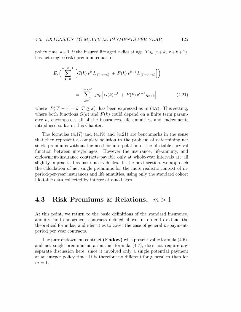
4.3. EXTENSION TO MULTIPLE PAYMENTS PER YEAR 125
policy time k+1 if the insured life aged x dies at age T ∈ [x+k, x+k+1),has net single (risk) premium equal to
Ex
( ω−x−1∑
k=0
[G(k) vk IT≥x+k + F (k) vk+1 I[T−x]=k
])
=ω−x−1∑
k=0
kpx
[G(k) vk + F (k) vk+1 qx+k
](4.21)
where P ([T − x] = k |T ≥ x) has been expressed as in (4.2). This setting,where both functions G(k) and F (k) could depend on a finite term param-eter n, encompasses all of the insurances, life annuities, and endowmentsintroduced so far in this Chapter.
The formulas (4.17) and (4.19) and (4.21) are benchmarks in the sensethat they represent a complete solution to the problem of determining netsingle premiums without the need for interpolation of the life-table survivalfunction between integer ages. However the insurance, life-annuity, andendowment-insurance contracts payable only at whole-year intervals are allslightly impractical as insurance vehicles. In the next section, we approachthe calculation of net single premiums for the more realistic context of m-period-per-year insurances and life annuities, using only the standard cohortlife-table data collected by integer attained ages.
4.3 Risk Premiums & Relations, m > 1
At this point, we return to the basic definitions of the standard insurance,annuity, and endowment contracts defined above, in order to extend thetheoretical formulas, and identities to cover the case of general m-payment-period per year contracts.
The pure endowment contract (Endow) with present value formula (4.6),and net single premium notation and formula (4.7), does not require anyseparate discussion here, since it involved only a single potential paymentat an integer policy time. It is therefore no different for general m than form = 1.

126 CHAPTER 4. EXPECTED PRESENT VALUES OF PAYMENTS
Next we consider the pure term insurance (Insm) with term n and mpayment periods per year, and level face amount. Recall that this contract,with unit face amount, pays 1 at the end of the 1/m year of death, ifdeath occurs before policy time n. That is, the payment of 1 occurs atpolicy time k/m if k/m ≤ T − x < (k + 1)/m, k/m < n. Accordingly,the present value of the insurer’s payment is
nm−1∑
k=0
v(k+1)/m Ik/m≤T−x<(k+1)/m (4.22)
and the net single premium or expected present value is
A(m)1x:n =
nm−1∑
k=0
v(k+1)/mk/mpx 1/mqx+k/m (4.23)
Here k/m in the summation formula denotes the beginning of the 1/myear of policy time within which death is to occur. Again the risk premiumsummation is the weighted sum, over all indices k such that k/m < n, ofthe present values v(k+1)/m to be paid by the insurer in the event that thepolicy age at death falls in [k/m, (k + 1)/m) multiplied by the probability,given in formula (4.3), that this event occurs.
To figure the expected present value of the life annuity-due with term n,note that payments of 1/m occur at all policy ages k/m, k = 0, . . . , nm−1,for which T − x ≥ k/m. Therefore, since the present values of thesepayments are (1/m) vk/m and the payment at k/m is made with probability
k/mpx ,
a(m)x:n = Ex
(nm−1∑
k=0
1
mvk/m I[T−x≥k/m]
)=
1
m
nm−1∑
k=0
vk/mk/mpx (4.24)
The useful identities described in Section 4.2.1 above, connecting thedifferent types of risk premiums for contracts with m = 1 payment periodper year, all have extensions to general m payment per year contracts.
The first extension, analogous to (4.10), is the definition of endowmentinsurance as the superposition of a constant-face-amount term insurance witha pure endowment of the same face amount and term. Recall that the m-payment-period per year endowment insurance with term n and unit face

4.3. EXTENSION TO MULTIPLE PAYMENTS PER YEAR 127
amount pays 1 at policy time (k +1)/m if k/m ≤ T −x < (k +1)/m fork = 0, 1, . . . , nm − 1, and pays 1 at policy time n if T ≥ x + n. Thepresent value of the payout clearly has the single epxression vmin(Tm−x+1/m, n).In terms of net single premiums, the notational identity is
A(m)x:n = A(m)1
x:n + A(m) 1x:n =
m(ω−x)−1∑
k=0
vmin((k+1)/m,n)k/mpx 1/mqx+k/m
(4.25)
=
nm−1∑
k=0
v(k+1)/mk/mpx 1/mqx+k/m + vn
npx
Again we find a formula for the endowment insurance by a combining theidentity (4.25) with the formula (4.23) for Insurance:
A(m)x:n =
nm−1∑
k=0
v(k+1)/m(
k/mpx − (k+1)/mpx
)+ vn
npx (4.26)
The general identity (4.11) concerning the relation between expectedpresent values of endowment insurances and life annuities also extends straight-forwardly. With m payments per year, and the individual payments of 1/magain totalling 1 per year, the term-n life annuity-due payout is given viaformula (2.4) by
a(m)
min(Tm−x+1/m, n)= (1 − vmin(Tm−x+1/m, n)) / d(m)
Again the unit life annuity-due has present value which is a simple linear func-tion of the present value vmin(Tm−x+1/m, n) of the unit endowment insurance.Taking expectations (over values of the random variable T , conditionallygiven T ≥ x) in the present value formula, and substituting the notation
A(m)x:n then yields:
a(m)x:n = Ex
(1 − vmin(Tm−x+1/m, n)
d(m)
)=
1 − A(m)x:n
d(m)(4.27)
where recall that Ex( · ) denotes the conditional expectation E( · |T ≥ x).An algebraically equivalent form of the identity (4.27) is
d(m) a(m)x:n + A
(m)x:n = 1 (4.28)

128 CHAPTER 4. EXPECTED PRESENT VALUES OF PAYMENTS
For multiple payment periods per year, the idea for converting from riskpremiums of life annuities-due to life annuities immediate is very similar tothe idea behind the conversion formula (4.13) for m = 1. The paymentstream for the unit annuity-immediate to a life aged x with payment of 1 peryear, term n years, and m payments per year consists of payments 1/mat each of the policy times k/m such that 1 ≤ k ≤ nm and k/n ≤ T −x.The corresponding payment stream for an annuity-due with term n + 1/mis exaxtly the same, except that the latter omits the initial payment of 1/m
at time 0. Therefore the respective expected present values a(m)x:n and
a(m)
x:n+1/mdiffer by exactly the present value of that initial payment of 1/m,
establishing the identity
a(m)x:n = a
(m)
x:n+1/m− 1
m= Ex
(a
(m)
min(Tm−x,n)+1/m
)(4.29)
From this m-payment-period conversion formula, we directly obtain an iden-tity relating the net single premium for life annuities-immediate with mpayment periods per year to that of the m payment period endowmentinsurances. The result is
a(m)x:n = a
(m)
x:n+1/m− 1
m=
1 −A(m)
x:n+1/m
d(m)− 1
m=
1
i(m)− 1
d(m)A
(m)
x:n+1/m(4.30)
and
d(m) a(m)x:n + A
(m)
x:n+1/m=
d(m)
i(m)= v1/m (4.31)
In these formulas, we have made use of the definition
m/d(m) = (1 + i(m)/m)/
(i(m)/m)
leading to the simplifications
m
d(m)=
m
i(m)+ 1 ,
i(m)
d(m)= 1 +
i(m)
m= v−1/m
We conclude this section with a general formula extending (4.21). Acontract which, for all integers k = 0, 1, . . . , m(ω−x)−1, pays 1
mGx(k/m)
at policy time k/m if the insured life initially aged x survives to age x+k/m,

4.3. EXTENSION TO MULTIPLE PAYMENTS PER YEAR 129
and which pays Fx(k/m) at policy time (k + 1)/m if the insured life agedx dies within the exact-age interval T ∈ [x + k/m, x + (k + 1)/m), has netsingle (risk) premium equal to
Ex
(m(ω−x)−1∑
k=0
[ 1
mGx(k/m) vk/m IT−x≥k/m +Fx(k/m) v(k+1)/m ITm−x=k/m
])
=
m(ω−x)−1∑
k=0
k/mpx
[ 1
mGx(k) vk/m + Fx(k/m) v(k+1)/m
1/mqx+k/m
](4.32)
See the Worked Examples (numbers 3 and 4) for illustrations of numericalcalculations with the standard formulas (4.22) and (4.24), as well as thegeneral formula (4.32).
The idea behind equation (4.32) can also be used to express the net singlepremium of a life insurance or annuity in a varying interest rate environment.Following the ideas of Sections 1.2.4 and 1.2.5, we know that the presentvalueof a unit payment at policy time t under a time-varying instantaneousinterest rate r(s) ≡ exp(δ(s)) − 1 (expressed in terms of the policy time-argument s) is 1/A(t) = exp(−
∫ t
0δ(s) ds). Then the present value of a
term insurance of duration n with level payment amount F at policytime (k + 1)/m if the insured life aged x dies within the exact-age intervalT ∈ [x + k/m, x + (k + 1)/m), 0 ≤ k < nm, is given by
F · exp(−∫ (k+1)/m
0
δ(s) ds)
ITm=x+k/m =F
A((k + 1)/m)Ik/m≤T−x<(k+1)/m
Similarly, the present value of a temporary life annuity due of duration nwhich makes level payments of amount 1
mG at all policy times k/m ≤
min(T − x, n), is
G
m·
nm−1∑
j=0
exp(−∫ j/m
0
δ(s) ds)
Ij/m≤T−x =G
m
nm−1∑
j=0
1
A(k/m)Ij/m≤T−x
Then the net single premium of a contract which pays G/m at policy timek/m ≤ n if the insured life initially aged x survives to age x + k/m, andwhich pays F at policy time (k + 1)/m ≤ n if the insured life aged x

130 CHAPTER 4. EXPECTED PRESENT VALUES OF PAYMENTS
dies within the exact-age interval T ∈ [x + k/m, x + (k + 1)/m), is theexpectation of the sum of the last two displayed expressions, and is given by
nm−1∑
k=0
k/mpx
[ G
m · A(k/m)+
F
A((k + 1)/m)1/mqx+k/m
](4.33)
4.4 Interpolation Formulas in Risk Premiums
A key issue in understanding the special nature of life insurances and annu-ities with multiple payment periods is the calculation of these probabilitiesfrom the underlying probabilities jpy (for integers j, y) which can be de-duced or estimated from life-tables. In the present Section, we combine theActuarial Assumption — (i) of Chapter 3, saying that deaths are uniformlydistributed within whole year of age — with the insurance and (temporary)life annuity-due risk premium formulas. In this setting, the number m ofpayment periods per year is greater than 1, and by formula (3.23) for allintegers j = 0, 1, . . . ,m − 1:
j/mpx = 1 − j/mqx = 1 − (j/m) qx
so that
j/mpx 1/mqx+j/m = j/mpx − (j+1)/mpx = (1/m) qx
For any integer k = bm + j, where 0 ≤ l < m− 1 and b is an integer,
k/mpx 1/mqx+k/m = bpx ( j/mpx+b − (j+1)/mpx+b) = (1/m) bpx qx+b (4.34)
Substituting (4.34) into (4.23) with summation indices k = bm+j, gives
A(m)1x:n =
n−1∑
b=0
m−1∑
j=0
vb+(j+1)/mb+j/mpx 1/mqx+b+j/m
=1
m
n−1∑
b=0
vbbpx qx+b
m−1∑
j=0
v(j+1)/m
=( 1
m
m−1∑
j=0
v(j+1)/m)· (1 + i)
( n−1∑
b=0
vb+1bpx qx+b
)

4.4. INTERPOLATION FORMULAS IN RISK PREMIUMS 131
The two factors in parentheses in the final displayed expression are respec-tively the one-year annuity-immediate present value a
(m)
1and the one-
payment-per-year term insurance risk-premium A1x:n . Since
(1 + i) a(m)
1= (1 + i) (1 − v)/i(m) = i/i(m)
it follows that under interpolation assumption (i),
A(m)1x:n = (i/i(m))
n−1∑
b=0
vb+1bpx qx+b = (i/i(m))A1
x:n (4.35)
Similarly, formula (4.34) substituted into the temporary life annuity for-mula (4.24) with summation index k = bm + j gives
a(m)x:n =
1
m
n−1∑
b=0
m−1∑
j=0
vb+j/mj/mpx+b · bpx =
1
m
n−1∑
b=0
vbbpx
m−1∑
j=0
vj/m (1− j
mqx+b)
=1
m
m−1∑
j=0
vj/m ax:n − 1 + i
m2
(m−1∑
j=0
j vj/m)
A1x:n (4.36)
This formula can be reduced further in either of two ways. First, one canappeal to the definition of increasing temporary annuity-due and refer to theformula given in paragraph (iv) of Section 2.1.1:
1
m2
m−1∑
j=0
j vj/m =1
m2
m−1∑
j=0
(j + 1) vj/m − 1
ma
(m)
1
= (I(m)a)(m)
1− 1 − v
md(m)=
1
d(m)
(1 − v
d(m)− v − 1 − v
m
)(4.37)
Alternatively, using the identity
A(m)x:n = A(m)1
x:n + vnnpx
within (4.27), and directly substituting (4.35), yields under (i)
a(m)x:n =
1
d(m)
(1 − i
i(m)A1
x:n − vnnpx
)(4.38)
We leave as an Exercise for the interested reader to verify algebraically, using(4.37) together with (4.11), that the formulas (4.36) and (4.38) are equal.

132 CHAPTER 4. EXPECTED PRESENT VALUES OF PAYMENTS
4.5 Continuous Risk Premium Formulas
The present chapter has developed formulas for the net single premiums orrisk premiums of the principal life insurance and annuity contracts, first inthe setting of one payment period per year (m = 1) and then in the caseof multiple payment periods (m > 1) per year. In the limit as m getslarge, the risk premium formulas become expected present values calculatedas continuous integrals with respect to survival densities. To recall why thislimit exists, note that for any function g(T ) which depends on T onlythrough the last completed 1/m’th year Tm = [Tm]/m,
Ex(g(T )) =
m(ω−x)−1∑
k=0
g(x + k/m) k/mpx 1/mpx+k/m
where we have used (4.3) as the probability mass function for Tm. Thedisplayed expectation formula is then also valid with m replaced by anyinteger multiple M = mn, n ≥ 1, and has the equivalent expression
M(ω−x)−1∑
k=0
g(x + k/M)
S(x)
∫ x+(k+1)/M
x+k/M
f(t) dt
=1
S(x)
M(ω−x)−1∑
k=0
∫ x+(k+1)/M
x+k/M
g(t) f(t) dt =
∫ ω−x
0
g(x + s)f(x + s)
S(x)ds
Assume now that the function g(t) is continuous (and therefore uniformlycontinuous) on the bounded lifetime interval [0, ω], so that g(t)−g([tM ]/Mcan be made uniformly small by choice of a sufficiently large multiple M ofm. Since the displayed expectation formulas are exactly valid when appliedto the function g([tM ]/M , it follows also for the general continuous functiong that
Ex(g(T )) = limM→∞
Ex(g(TM)) =
∫ ω−x
0
g(x + s)f(x + s)
S(x)ds (4.39)
or, with the substitution f(x + s) = µ(x + s)S(x + s),
Ex(g(T )) =
∫ ω−x
0
g(x + s)µ(x + s)S(x + s)
S(x)ds (4.40)

4.5. CONTINUOUS RISK PREMIUM FORMULAS 133
Similar justifications can be given for these expectation formulas also when-ever g is piecewise continuous. These integral formulas can be used eitherto calculate the limiting values of expected present values for insurance con-tracts with large m, or to calculate other expectations of demographic andbiostatistical interest, such as life expectancies.
4.5.1 Continuous Insurance Contracts
So far in this Chapter, all of the expectations considered have been associ-ated with the discretized random lifetime variables [T ] and Tm = [mT ]/m.However, Insurance and Annuity contracts can also be defined with re-spectively instantaneous and continuous payments, as follows. First, aninstantaneous-payment or continuous insurance with face-value Fis a contract which pays an amount F at the instant of death of the in-sured. (In practice, this means that when the actual payment is made atsome later time, the amount paid is F together with interest compoundedfrom the instant of death.) As a function of the random lifetime T forthe insured life initially with exact integer age x, the present value of theamount paid is F · vT−x for a whole-life insurance and F · vT−x · I[T<x+n]
for an n-year term insurance. The expected present values or net single pre-miums on a life aged x are respectively denoted Ax for a whole-life contractand A1
x:n for an n-year term insurance. The continuous life annuity isa contract which provides continuous payments at rate 1 per unit time forduration equal to the smaller of the remaining lifetime of the annuitant orthe term of n years. Here the present value of the contractual payments,as a function of the exact age T at death for an annuitant initially of exactinteger age x, is amin(T−x,n) where n is the (possibly infinite) durationof the life annuity. Recall that
aK =
∫ ∞
0
vt I[t≤K] dt =
∫ K
0
vt dt = (1 − vK)/δ
is the present value of a continuous payment stream of 1 per unit time ofduration K units, where v = (1 + i)−1 and δ = ln(1 + i) . The actuarialnotation for the net single premium of the temporary continuous life annuityis ax:n which simplifies to ax when n = ∞.
The objective of this section is to develop and interpret formulas for the

134 CHAPTER 4. EXPECTED PRESENT VALUES OF PAYMENTS
continuous-time net single premiums, along with one further quantity whichhas been defined as a continuous-time expectation of the lifetime variable T ,namely the mean residual life (also called complete life expectancy)ex = Ex(T − x) for a life aged x.
4.5.2 Integral Formulas
We apply the continuous conditional expectation formulas (4.39) or (4.40)directly for the three choices
g(y) = y − x , vy−x , or vy−x · Iy−x<n
which respectively have the conditional Ex(·) expectations
ex , Ax , A1x:n
For easy reference, the integral formulas for these three cases are:
ex = Ex(T − x) =
∫ ∞
0
s µ(x + s) spx ds (4.41)
Ax = Ex(vT−x) =
∫ ∞
0
vs µ(x + s) spx ds (4.42)
A1x:n = Ex
(vT−x IT−x≤n
)=
∫ n
0
vs µ(x + s) spx ds (4.43)
Next, we obtain two additional formulas, for continuous life annuities-due
ax and ax:n
which correspond to Exg(T ) for the two choices
g(t) =
∫ ω−x
0
vy Iy+x≤t dy or
∫ n
0
vy Iy+x≤t dy
where we naturally assume that x+n ≤ ω in the case of the temporary lifeannuity.

4.5. CONTINUOUS RISK PREMIUM FORMULAS 135
After switching the order of the integrals and the conditional expecta-tions, and evaluating the conditional expectation of an indicator as a condi-tional probability, in the form
Ex
(Iy≤T−x
)= P (T ≥ x + s |T ≥ x) =
S(x + y)
S(x)= ypx
the resulting two equations become
ax = Ex
(∫ ω−x
0
vy Iy≤T−x dt
)=
∫ ω−x
0
vyypx dy (4.44)
ax:n = Ex
(∫ n
0
vy Iy≤T−x dy
)=
∫ n
0
vyypx dy (4.45)
As seen above in (4.39), risk premiums for continuous insurance and an-nuity contracts have a close relationship to the corresponding contracts withm payment periods per year for large m. That is, the term insurance netsingle premiums
A(m)1x:n = Ex
(vTm−x+1/m
)
approach the continuous insurance value (4.42) as a limit when m → ∞.A simple direct proof can be given because the payments at the end of thefraction 1/m of year of death are at most 1/m years later than thecontinuous-insurance payment at the instant of death, so that the followingobvious inequalities hold:
A1x:n ≤ A(m)1
x:n ≤ v1/m A1x:n (4.46)
Since the right-hand term in the inequality (4.46) also converges for large mto the leftmost term, the middle term which is sandwiched in between mustconverge to the same limit (4.43).
For the continuous annuity, (4.45) can be obtained as a limit of formulas(4.19) either from (4.39) or by using Riemann sums, as the number m ofpayments per year goes to ∞, i.e.,
ax:n = limm→∞
a(m)x:n = lim
m→∞
nm−1∑
k=0
1
mvk/m
k/mpx =
∫ n
0
vttpx ds
The final formula coincides with (4.45), according with the intuition that thelimit as m → ∞ of the payment-stream which pays 1/m at intervals of time

136 CHAPTER 4. EXPECTED PRESENT VALUES OF PAYMENTS
1/m between 0 and Tm − x inclusive is the continuous payment-streamwhich pays 1 per unit time throughout the policy-age interval [0, T − x).
The limiting argument of the previous paragraph shows immediately thatunder interpolation assumption (i), there are simple formulas relating Ax:n
and ax:n to A1x:n . Indeed, by (4.35), under (i)
Ax:n = limm→∞
A(m)1x:n = lim
m
i
i(m)A1
x:n =i
δA1
x:n (4.47)
and by (4.38), also under (i),
ax:n = limm→∞
a(m)x:n = lim
m
1
d(m)
(1 − i
i(m)A1
x:n − vnnpx
)
or
ax:n =1
δ
(1 − i
δA1
x:n − vnnpx
)(4.48)
Finally, it is easy to see by passing to the limit m → ∞ in (4.28) that
δ ax:n + Ax:n = 1 (4.49)
More elaborate relations will be given in the next Chapter between netsingle premium formulas which do require interpolation-assumptions for prob-abilities of survival to times between integer ages to formulas for m = 1,which do not require such interpolation.
The expressions in formulas (4.41), (4.43), and (4.45) can be contrastedwith the respective expectations (3.12), (4.17) and (4.19) for a function ofthe integer-valued random variable [T ] (taking m = 1). In particular,the complete life expectancy ex in (4.41) is compared to the curtate lifeexpectancy ex under interplation assumption (i) in (3.28). The comparisonbetween complete and curtate life expectancies under more general within-year survival distributions in subsection 4.5.4 below.
4.5.3 Risk Premiums under Theoretical Models
Let us work out examples of the multiple time-period per year and continuousformulas analytically and numerically, under a particular theoretical survivalmodel.

4.5. CONTINUOUS RISK PREMIUM FORMULAS 137
Consider first the slightly artificial (but still useful) case where theresidual life T − x for a life aged x is precisely Weibull(γ, λ) distributed,with force of mortality for T given by µ(x + s) = λ γ sγ−1, and
spx = e−λsγ
for all s ≥ 0 , qx+k = 1 − exp(−λ(k + 1)γ − kγ)
Then respectively according to formulas (4.17), (4.23), and (4.42), we findformulas for term-insurance finite-m net single premiums under Weibullsurvival as follows:
A1x:n =
n−1∑
k=0
vk+1 (e−λkγ − e−λ(k+1)γ
)
A(m)1x:n =
n−1∑
k=0
vk+1/mm−1∑
j=0
vj/m (e−λ(k+j/m)γ − e−λ(k+(j+1)/m)γ
)
According to formulas (4.19), (4.24), and (4.44), the special Weibull-lifetimetemporary life annuity-due risk premiums for finite m are:
ax:n =n−1∑
k=0
vk e−λ kγ
, a(m)x:n =
n−1∑
k=0
m−1∑
j=0
vk+j/m e−λ (k+j/m)γ
The continuous cases (m = ∞) of these formulas are as follows:
A1x:n =
∫ n
0
vs λγ sγ−1 e−λsγ
ds , ax:n =
∫ n
0
vs e−λsγ
ds
Finally, according to formulas (3.11) and (4.41) the curtate and completelife expectancies at integer ages y ≥ x for Weibull (residual) lifetimes are:
ex =∞∑
k=0
k (e−λkγ − e−λ(k+1)γ
) , ex =
∫ ∞
0
s λγ sγ−1 eλsγ
ds
We next give R code and a table showing some numerical comparisons ofthese insurance and life-annuity risk premiums, for m = 1, 4, ∞. First, wegive an R function for Weibull-lifetime term insurance risk premiums:

138 CHAPTER 4. EXPECTED PRESENT VALUES OF PAYMENTS
> WeibIns = function(lambda, gamma, m, n, i)
## Function to calculate term-n insurance risk prem
### for 1 paymt per year, m paymts, and continuous ins
v = 1/(1+i)
xk = 0:(n-1)
Ins1 = v*sum( v^xk*(exp(-lambda*xk^gamma)-
exp(-lambda*(xk+1)^gamma)) )
xkjm = (0:(n*m-1))/m
Insm = v^(1/m)* sum( v^xkjm*(exp(-lambda*xkjm^gamma) -
exp(-lambda*(xkjm+1/m)^gamma)) )
InsC = lambda*gamma*integrate(function(s,.v,.lam,.gam)
.v^s*s^(.gam-1)*exp(-.lam*s^(.gam)),0, n,
.v=v, .lam=lambda, .gam=gamma)$val
c(termIns.1 = Ins1, termIns.m = Insm, termIns.cont = InsC)
To illustrate the use of this function, we create a small Table of valuesfor a few different values of n, with parameters (λ, γ) similar to thoseused in Chapter 2, but chosen successively so that (a) 32p40 = .5/.925 =.5405, 50p40 = .04/.925 = .04324 as in Figure 2.5, (b) 32p40 = .6, 50p40 =.047, or (c) 32p40 = .65, 50p40 = .05. In each case, the nominal age x is40, in the R code to produce this Table, we begin by coding a function tosolve for λ, γ) when π1 = 32p40, π2 = 50p40 are given. The interest ratesconsidered here are 0.05 or 0.06, and n = 20.
> LamGam = function(pi1,pi2, age1, age2)
### Function to solve for lambda and gamma Weibull
### parameters, when S(age1)=pi1, S(age2)=pi2 are fixed.
haz1 = -log(pi1) ; haz2 = -log(pi2)
gam = log(haz2/haz1)/log(age2/age1)
lam = haz1/age1^gam
c(lambda=lam, gamma=gam)
> LamGam(.5/.925,.04/.925,32,50)
lambda gamma
1.952e-06 3.653e+00

4.5. CONTINUOUS RISK PREMIUM FORMULAS 139
> WeibIns(1.952e-6,3.653,4,20,.05)
termIns.1 termIns.m termIns.cont
0.04844 0.04930 0.04960
> InsArr = array(0, dim=c(6,6), dimnames=list(NULL, c("lambda",
"gamma", "i", "Ins.1", "Ins.m", "Ins.C")))
intrat = c(.05, .06)
sprobs = rbind(c(.5/.925,.04/.925),c(.6,.047),c(.65,.05))
for(a in 1:2) for (b in 1:3)
k = 2*(b-1)+a
> lamgam=LamGam(sprobs[b,1],sprobs[b,2],32,50)
InsArr[k,] = c(lamgam[1],lamgam[2],intrat[a],
WeibIns(lamgam[1],lamgam[2],4,20,intrat[a]))
InsArr
lambda gamma i Ins.1 Ins.m Ins.C
[1,] 1.952e-06 3.653 0.05 0.04846 0.04932 0.04962
[2,] 1.952e-06 3.653 0.06 0.04189 0.04278 0.04309
[3,] 4.715e-07 4.009 0.05 0.03396 0.03457 0.03478
[4,] 4.715e-07 4.009 0.06 0.02924 0.02986 0.03008
[5,] 1.241e-07 4.345 0.05 0.02436 0.02479 0.02494
[6,] 1.241e-07 4.345 0.06 0.02091 0.02135 0.02151
The variations among the parameters and interest rates make much moredifference to the results than does the number m of payment periods peryear. Note that the overall size of the risk premium for a unit 20-year terminsurance is reasonable, because the probability it will pay anything at all is
20q40, which (for odd-numbered rows) takes the three values
> 1-exp(-AnnuArr[c(1,3,5),1]*20^AnnuArr[c(1,3,5),2])
[1] 0.10461 0.07467 0.05435
A similar Table of risk premiums for temporary life annuities-due, withexactly the same parameters, is given below along with the R code for thelife-annuity function calculation.

140 CHAPTER 4. EXPECTED PRESENT VALUES OF PAYMENTS
> WeibAnnD = function(lambda, gamma, m, n, i)
## Function to calculate term-n insurance risk prem
### for 1 paymt per year, m paymts, and continuous ins
v = 1/(1+i)
xk = 0:(n-1)
Annu1 = sum( v^xk*exp(-lambda*xk^gamma) )
xkjm = (0:(n*m-1))/m
Annum = sum( v^xkjm*exp(-lambda*xkjm^gamma) )/m
AnnuC = integrate(function(s,.v,.lam,.gam)
.v^s*exp(-.lam*s^(.gam)),0, n,
.v=v, .lam=lambda, .gam=gamma)$val
c(tmpAnn.1 = Annu1, tmpAnn.m = Annum, tmpAnn.cont = AnnuC)
> AnnuArr = InsArr
dimnames(AnnuArr)[[2]][4:6]=c("Annu.1","Annu.m","Annu.C")
for(a in 1:2) for (b in 1:3)
k = 2*(b-1)+a
lamgam=LamGam(sprobs[b,1],sprobs[b,2],32,50)
AnnuArr[k,4:6] = WeibAnnD(lamgam[1],lamgam[2],4,20,intrat[a])
AnnuArr
lambda gamma i Annu.1 Annu.m Annu.C
[1,] 1.952e-06 3.653 0.05 12.90 12.65 12.56
[2,] 1.952e-06 3.653 0.06 11.99 11.72 11.63
[3,] 4.715e-07 4.009 0.05 12.96 12.72 12.64
[4,] 4.715e-07 4.009 0.06 12.05 11.78 11.69
[5,] 1.241e-07 4.345 0.05 13.00 12.76 12.68
[6,] 1.241e-07 4.345 0.06 12.09 11.82 11.73
Life expectancy calculations and comparisons are done in the next sub-section, for Gompertz survival. Examples of formula development for otherspecial parametric distributional families are contained in the Exercises.
4.5.4 Numerical Calculations of Life Expectancies
Formulas (4.41) or (3.12) respectively provide the complete and curtate age-specific life expectancies, in terms respectively of survival densities and life-

4.5. CONTINUOUS RISK PREMIUM FORMULAS 141
table data. Formula (3.28) provides the actuarial approximation for com-plete life expectancy in terms of life-table data, based upon interpolation-assumption (i) (Uniform mortality within year of age). In this Section, weillustrate these formulas using the Illustrative simulated and extrapolatedlife-table data of Table 1.1.
Life expectancy formulas necessarily involve life table data and/or sur-vival distributions specified out to arbitrarily large ages. While life tablesmay be based on large cohorts of insured for ages up to the seventies and eveneighties, beyond that they will be very sparse and very dependent on the par-ticular small group(s) of aged individuals used in constructing the particulartable(s). On the other hand, the fraction of the cohort at moderate ages whowill survive past 90, say, is extremely small, so a reasonable extrapolationof a well-established table out to age 105 or so may give sufficiently accu-rate life-expectancy values at ages not exceeding 105. Life expectancies arein any case forecasts based upon an implicit assumption of future mortalityfollowing exactly the same pattern as recent past mortality. Life-expectancycalculations necessarily ignore likely changes in living conditions and medi-cal technology which many who are currently alive will experience. Thus anassertion of great accuracy for a particular method of calculation would bemisplaced.
All of the numerical life-expectancy calculations produced for the Figureof this Section are based on the extrapolation (2.10) of the illustrative lifetable data from Table 1.1. According to that extrapolation, death-rates qx
for all ages 78 and greater are taken to grow exponentially, with log(qx/q78) =(x − 78) ln(1.0885). This exponential behavior is approximately but notprecisely compatible with a Gompertz-form force-of-mortality function
µ(78 + t) = µ(78) ct
in light of the approximate equality µ(x) ≈ qx, an approximation whichprogressively becomes less valid as the force of mortality gets larger. To seethis, note that under a Gompertz survival model,
µ(x) = Bcx , qx = 1 − exp
(−Bcx c − 1
ln c
)
and with c = 1.0885 in our setting, (c − 1)/ ln c = 1.0436.

142 CHAPTER 4. EXPECTED PRESENT VALUES OF PAYMENTS
Since curtate life expectancy (3.12) relies directly on (extrapolated) life-table data, its calculation is simplest and most easily interpreted. Figure 4.1presents, as plotted points, the age-specific curtate life expectancies for in-teger ages x = 0, 1, . . . , 78. Since the complete life expectancy at each ageis larger than the curtate by exactly 1/2 under interpolation assumption(i), we calculated for comparison the complete life expectancy at all (real-number) ages, under assumption (ii) (from Chapter 3, as in equation 3.16)of piecewise-constant force of mortality within years of age. Under this as-sumption, by formula (3.24), mortality within year of age (0 < t < 1) is
tpx+k = (px+k)t, and force of mortality is
µ(x + k + t) = − d
dtln tpx+k = − ln px+k
Using formulas (4.41), (3.12), and interpolation assumption (ii), the exactformula for the difference between complete and curtate life expectancy be-comes
ex − ex =
ω−x−1∑
k=0
kpx
∫ k+1
k
s µ(x + s) s−kpx+k ds − k qx+k
=ω−x−1∑
k=0
kpx
(− ln px+k)
∫ 1
0
(k + t) et lnpx+k dt − k qx+k
=
ω−x−1∑
k=0
kpx
(− ln px+k)
((k + 1)px+k − k
ln px+k− px+k − 1
(ln px+k)2
)− k qx+k
=ω−x−1∑
k=0
kpx
(− px+k − qx+k
ln px+k
)(4.50)
The complete minus curtate life expectancies calculated from this formulawere found range from 0.493 at ages 40 and below, down to 0.485 at age78 and 0.348 at age 99. (Contrast this result with the constant differenceof 1/2 under assumption (i).) Thus there is essentially no new informationin the calculated complete life expectancies, and they are not plotted.
The aspect of Figure 4.1 which is most startling to the intuition is thelarge expected numbers of additional birthdays for individuals of advancedages. Moreover, the large life expectancies shown are comparable to actualUS male mortality circa 1959, so would be still larger today.

4.5. CONTINUOUS RISK PREMIUM FORMULAS 143
• • • • • • • • • • • • • • • • • • • • • • • • • • • • • • • • • • • • • • • • • • • • • • • • • • • • • • • • • • • • • • • • • • • • • • • • • • • • • • •
Expected number of additional whole years of life, by age
Age in years
Cur
tate
Life
Exp
ecta
ncy
0 20 40 60 80
1020
3040
5060
70
Figure 4.1: Curtate life expectancy ex as a function of age, calculatedfrom the simulated illustrative life table data of Table 1.1, with age-specificdeath-rates qx extrapolated as indicated in formula (2.10).

144 CHAPTER 4. EXPECTED PRESENT VALUES OF PAYMENTS
4.6 Exercise Set 4
(1). For each of the following three lifetime distributions, find (a) theexpected remaining lifetime for an individual aged 20, and (b) 7/12q40/q40.
(i) Weibull(.00634, 1.2), with S(t) = exp(−0.00634 t1.2),
(ii) Lognormal(log(50), 0.3252), with S(t) = 1−Φ((log(t)− log(50))/0.325),
(iii) Piecewise exponential with force of mortality given the constant valueµt = 0.015 for 20 < t ≤ 50, and µt = 0.03 for t ≥ 50. In theseintegrals, you should be prepared to use integrations by parts, gamma functionvalues, tables of the normal distribution function Φ(x), and/or numericalintegrations via calculators or software.
(2). (a) Find the expected present value, with respect to the constanteffective interest rate r = 0.07, of an insurance payment of $1000 to bemade at the instant of death of an individual who has just turned 40 andwhose remaining lifetime T − 40 = S is a continuous random variable withdensity f(s) = 0.05 e−0.05 s , s > 0.
(b) Find the expected present value of the insurance payment in (a) ifthe insurer is allowed to delay the payment to the end of the year in whichthe individual dies. Should this answer be larger or smaller than the answerin (a) ?
(3). If the individual in Problem 2 pays a life insurance premium P atthe beginning of each remaining year of his life (including this one), thenwhat is the expected total present value of all the premiums he pays beforehis death ?
(4). Suppose that an individual has equal probability of dying within eachof the next 40 years, and is certain to die within this time, i.e., his age is xand
kpx − k+1px = 0.025 for k = 0, 1, . . . , 39
Assume the fixed interest rate r = 0.06.
(a) Find the net single whole-life insurance premium Ax for this person.
(b) Find the net single premium for the term and endowment insurancesA1
x:20and Ax:30 .

4.6. EXERCISE SET 4 145
(5). Show that the expected whole number of years of remaining life for alife aged x is given by
cx = E([T ]− x | T ≥ x) =
ω−x−1∑
k=0
k kpx qx+k
and prove that this quantity as a function of integer age x satisfies therecursion equation
cx = px (1 + cx+1)
(6). Show that the expected present value bx of an insurance of 1 payableat the beginning of the year of death (or equivalently, payable at the end ofthe year of death along with interest from the beginning of that same year)satisfies the recursion relation (4.51) above.
(7). Prove the identity (4.16) algebraically.
For the next two problems, consider a cohort life-table population forwhich you know only that l70 = 10, 000, l75 = 7000, l80 = 3000, l85 = 0, andthat the distribution of death-times within 5-year age intervals is uniform.
(8). Find (a) e75 and (b) the probability of an individual aged 70 inthis life-table population dying between ages 72.0 and 78.0.
(9). Find the probability of an individual aged 72 in this life-table popula-tion dying between ages 75.0 and 83.0, if the assumption of uniform death-times within 5-year intervals is replaced by:
(a) a constant force of mortality within 5-year age-intervals;
(b) assuming linearity of 1/S(t)) within 5-year age intervals.
(10). Suppose that a population has survival probabilities governed at allages by the force of mortality
µt =
.01 for 0 ≤ t < 1
.002 for 1 ≤ t < 5
.001 for 5 ≤ t < 20
.004 for 20 ≤ t < 40
.0001 · t for 40 ≤ t
Then (a) find 30p10, and (b) find e50.

146 CHAPTER 4. EXPECTED PRESENT VALUES OF PAYMENTS
(11). Suppose that a population has survival probabilities governed at allages by the force of mortality
µt =
.01 for 0 ≤ t < 10
.1 for 10 ≤ t < 303/t for 30 ≤ t
Then (a) find 30p20 = the probability that an individual aged 20 survivesfor at least 30 more years, and (b) find e30.
(12). Assuming the same force of mortality as in the previous problem, finde70 and A60 if i = 0.09.
(13). The force of mortality for impaired lives is three times the standardforce of mortality at all ages. The standard rates qx of mortality at ages 95,96, and 97 are respectively 0.3, 0.4, and 0.5 . What is the probability thatan impaired life age 95 will live to age 98 ?
(14). You are given a survival function S(x) = (10−x)2/100 , 0 ≤ x ≤ 10.
(a) Calculate the average number of future years of life for an individualwho survives to age 1.
(b) Calculate the difference between the force of mortality at age 1, andthe probability that a life aged 1 dies before age 2.
(15). An n-year term life insurance policy to a life aged x providesthat if the insured dies within the n-year period an annuity-certain of yearlypayments of 10 will be paid to the beneficiary, with the first annuity paymentmade on the policy-anniversary following death, and the last payment made
on the N th policy anniversary. Here 1 < n ≤ N are fixed integers. IfB(x, n,N) denotes the net single premium (= expected present value) forthis policy, and if mortality follows the law lx = C(ω − x)/ω for someterminal integer age ω and constant C, then find a simplified expressionfor B(x, n,N) in terms of interest-rate functions, ω, and the integersx, n, N . Assume x + n ≤ ω.
(16). The father of a newborn child purchases an endowment and insurancecontract with the following combination of benefits. The child is to receive
$100, 000 for college at her 18th birthday if she lives that long and $500, 000
at her 60th birthday if she lives that long, and the father as beneficiary isto receive $200, 000 at the end of the year of the child’s death if the child

4.6. EXERCISE SET 4 147
dies before age 18. Find expressions, both in actuarial notations and interms of v = 1/(1 + i) and of the survival probabilities kp0 for the child,for the net single premium for this contract.
(17). Verify algebraically, using (4.37) together with (4.11), that the right-hand sides of formulas (4.36) and (4.38) are equal.
For the next four problems, concerning insurance contract risk premiumsin a variable interest rate environment, apply formula (4.33).
(18). Suppose that a life aged x wants to purchase a 20-year term insurancenow, and that interest rates over the next twenty years will be i = .05 forpolicy ages in (0, 10] and i = .06 for policy ages in (10, 20]. Find the netsingle premium for a unit term insurance (i.e., if the insurance payment is 1)if survival is governed by the Weibull(2 · 10−6, 4) distribution for T−x. (Youmay use the formulas and R code of section 4.5.3 to aid in the calculation.)
(19). Pass to the limit m → ∞ in formula (4.33) to derive an analogousformula for the net single premium, in a variable interest rate environmentwith instantaneous force of interest δ(t) at policy time t, of a contractfor a life aged x paying a continuous-time stream at rate G at all policytimes t < min(T − x, n) and paying a lump-sum amount F at the instantof death if death occurs before age x + n.
(20). Suppose that a life aged x wants to purchase a 10-year term insuranceor temporary annuity-due, and that interest rates over the next ten years willbe i = .07 for policy ages in (0, 6] and i = .04 for policy ages in (6, 10].Show that the net single premium for a unit 10-year term insurance or aunit temporary life annuity-due, with one payment period per year (i.e.,m = 1) depends on the survival distribution only through the cohort lifetable quantities kpx for integers k = 1, 2, . . . , 10.
(21). Suppose that a life aged x wants to purchase a 10-year term in-surance, and that it is believed that interest rates will vary over the 10-yearinterval according to the rule δ(t) = δ · (1 + 0.002 t). Show that the netsingle premium for a unit 10-year term insurance depends on the continuousconditional survival probabilities tpx, 0 ≤ t ≤ 10 and not only on the valuesfor integer t.

148 CHAPTER 4. EXPECTED PRESENT VALUES OF PAYMENTS
4.7 Worked Examples
Example 1. Toy Life-Table (assuming uniform failures)
Consider the following life-table with only six equally-spaced ages. (Thatis, assume l6 = 0.) Assume that the rate of interest i = .09, so thatv = 1/(1 + i) = 0.9174 and (1 − e−δ)/δ = (1 − v)/δ = 0.9582.
x Age-range lx dx ex Ax
0 [0, 1) 1000 60 4.2 0.7041 [1, 2) 940 80 3.436 0.7492 [2, 3) 860 100 2.709 0.7953 [3, 4) 760 120 2.0 0.8444 [4, 5) 640 140 1.281 0.8965 [5, 6) 500 500 0.5 0.958
Using the data in this Table, and interest rate i = .09, we begin by cal-culating the expected present values for simple contracts for term insurance,annuity, and endowment. First, for a life aged 0, a 3-year term insurancewith payoff amount $1000 has present value given by formula (4.17) as
1000A10:3 = 1000
0.917
60
1000+ (0.917)2 80
1000+ (0.917)3 100
1000
= 199.60
Second, for a life aged 2, a 3-year temporary annuity-due of $700 per year(with last payment at age 4) has present value computed from (4.19) to be
700 a2:3 = 700
1 + 0.917
760
860+ (0.917)2 640
860
= 1705.98
For the same life aged 2, the 3-year Endowment for $700 has present value
700A 12:3
= 700 · (0.9174)3 500
860= 314.26
Thus we can also calculate (for the life aged 2) the present value of the3-year annuity-immediate of $700 per year as
700 ·(a2:3 − 1 + A 1
0:3
)= 1705.98 − 700 + 314.26 = 1320.24

4.7. WORKED EXAMPLES 149
We next apply and interpret the formulas of Section 4.5.1, together withthe observation that
jpx · qx+j =lx+j
lx· dx+j
lx+j=
dx+j
lx
to show how the last two columns of the Table were computed. In particular,by (4.41)
e2 =100
860· 0 +
120
860· 1 +
140
860· 2 +
500
860· 3 +
1
2=
1900
860+ 0.5 = 2.709
Moreover: observe that cx =∑5−x
k=0 k kpxqx+k satisfies the “recursion equa-tion” cx = px (1 + cx+1) (cf. Exercise 5 above), with c5 = 0, from whichthe ex column is easily computed by: ex = cx + 0.5.
Now apply the present value formula for continuous insurance to find
Ax =5−x∑
k=0
kpx qx+k vk 1 − e−δ
δ= 0.9582
5−x∑
k=0
kpx qx vk = 0.9582 bx
where bx is the expected present value of an insurance of 1 payable at thebeginning of the year of death (so that Ax = v bx ) and satisfies b5 = 1together with the recursion-relation
bx =5−x∑
k=0
kpx qx+k vk = px v bx+1 + qx (4.51)
(Proof of this recursion is Exercise 6 above.)
Example 2. Find a simplified expression in terms of actuarial expectedpresent value notations for the net single premium of an insurance on alife aged x, which pays F (k) = C an−k if death occurs at any exact agesbetween x + k and x + k + 1, for k = 0, 1, . . . , n − 1, and interpret theresult.
Let us begin with the interpretation: the beneficiary receives at the endof the year of death a lump-sum equal in present value to a payment streamof C annually beginning at the end of the year of death and terminating at
the end of the nth policy year. This payment stream, if superposed upon

150 CHAPTER 4. EXPECTED PRESENT VALUES OF PAYMENTS
an n-year life annuity-immediate with annual payments C, would result ina certain payment of C at the end of policy years 1, 2, . . . , n. Thus theexpected present value in this example is given by
C an − C ax:n (4.52)
Next we re-work this example purely in terms of analytical formulas. Byformula (4.52), the net single premium in the example is equal to
n−1∑
k=0
vk+1kpx qx+k C an−k+1 = C
n−1∑
k=0
vk+1kpx qx+k
1 − vn−k
d
=C
d
n−1∑
k=0
vk+1kpx qx+k − vn+1
n−1∑
k=0
(kpx − k+1px)
=C
d
A1
x:n − vn+1 (1 − npx)
=C
d
Ax:n − vn
npx − vn+1 (1 − npx)
and finally, by substituting expression (4.15) with m = 1 for Ax:n , wehave
C
d
1 − d ax:n − (1 − v) vn
npx − vn+1
=C
d
1 − d (1 + ax:n − vn
npx) − d vnnpx − vn+1
=C
d
v − d ax:n − vn+1
= C
1 − vn
i− ax:n
= C an − ax:n
So the analytically derived answer agrees with the one intuitively arrived atin formula (4.52).
Example 3. Consider the following cohort life table fragment applicable tolives aged from 30 to 36. Find the risk premiums for unit-face-amount 6-yearduration annuity-due and term insurance, (a) with m=1, (b) with m = 4and uniform failure density within year of failure, and (c) with m = 4 andrespective failure probabilities .2, .2, .3, .3 of dying within the 4 quarter-yearsgiven the year of failure. Assume interest rate 5% throughout.

4.7. WORKED EXAMPLES 151
x Age-range lx dx
30 [30, 31) 95000 16531 [31, 32) 94835 15032 [32, 33) 94685 15533 [33, 34) 94530 15834 [34, 35) 94472 17235 [35, 36) 94300 187
To clarify the different calculations in the three parts (a)-(c), we provideR code as well as numerical answers. Parts (a) and (b) respectively make useof formulas (4.17), (4.19) and (4.35) plus (4.36).
> probmass = c(165,150,155,158,172,187)/95000
> kpx = 1-cumsum(c(0,probmass[1:5]))
> probmass
[1] 0.001737 0.001579 0.001632 0.001663 0.001811 0.001968
> kpx
[1] 1.0000 0.9983 0.9967 0.9951 0.9934 0.9916
> Ains = sum( 1.05^(-(1:6)) * probmass )
AnnDue = sum( 1.05^(-(0:5)) * kpx )
c(Ains=Ains, AnnDue=AnnDue)
Ains AnnDue
0.008751 5.308505 ### answer to (a)
> i4 = 4*(1.05^.25-1)
aux1 = sum(1.05^(-(0:3)/4))/4
aux2 = sum((0:3)*1.05^(-(0:3)/4))/4^2
c(Ains.m = Ains*i4/.05,
AnnDue.m = aux1*AnnDue - 1.05*aux2*Ains)
Ains.m AnnDue.m
0.008592 5.209397 ### answer to (b)
For part (c), we start from formulas (4.23) and (4.24) and calculate by de-composing sums as we did in Section 4.4,
A(m)1x:n =
n−1∑
b=0
bpx
m−1∑
j=0
vb+(j+1)/m ((j+1)/mqx+b − j/mqx+b)

152 CHAPTER 4. EXPECTED PRESENT VALUES OF PAYMENTS
a(m)x:n =
n−1∑
b=0
bpx1
m
m−1∑
j=0
vb+j/m (1 − j/mqx+b)
Now for m = 4, we have in this problem the special assumption that forintegers b and 0 ≤ j < 4,
(j/4qx+b − (j+1)/4qx+b)/qx+b =
0.2 if j = 0, 10.3 if j = 2, 3
It follows that j/4qx+b / qx+b has respective values 0, 0.2, 0.4, 0.7 for j =0, 1, 2, 3. Substituting, we find
A(4)1x:n =
n−1∑
b=0
bpx qx+b vb+1 (1 + i)(0.2 v1/4 + 0.2 v1/2 + 0.3 v3/4 + 0.3 v
)
= A1x:n ·
(0.2 v1/4 + +0.2 v1/2 + 0.3 v3/4 + 0.3 v
)(1 + i)
and
a(4)x:n =
1
4
n−1∑
b=0
bpx vb(1 − v qx+b (0.2 v−3/4 + 0.4 v−1/2 + 0.7 v−1/4)
)
= ax:n − 1
4A1
x:n
(0.2 v−3/4 + 0.4 v−1/2 + 0.7 v−1/4
)
The numerics in R for part (c) now follow:
> aux3 = .2*(1.05^.75+1.05^.5)+.3*(1.05^.25 + 1)
aux4 = .2*1.05^.75+.4*1.05^.5+.7*1.05^.25
c(Ains.ptc = Ains*aux3, AnnDue.ptc = AnnDue - 0.25*Ains*aux4
Ains.ptc AnnDue.ptc
0.008892 5.305604
So the different within-year distribution of failures made roughly a 2% dif-ference in the term insurance and temporary life annuity-due risk premiums.

4.7. WORKED EXAMPLES 153
Example 4. Find the risk premiums for a 24-year life annuity-due and insur-ance figured with m = 1 and m = 4 based on the probability densities, withparameters as given in Figure 2.5 in Chapter 2, (a) Gamma(14.74, .4383),and (b) Lognormal(3.491, (.246)2).
Here the ideas and formulas are simple: the only issue is how to organizethe numerical calculations. The Gamma distribution function can be directlycalled in R, while the Lognormal distribution function values are simply ex-pressed in terms of the normal distribution function. In neither case need weperform numerical integrations.
kpx1 = 1-pgamma(0:24, rate=.4383, shape=14.74)
kpx2 = 1-pnorm(log(0:24),mean=3.491, sd =.246)
array(c(sum(-diff(kpx1)/1.05^(1:24)),
sum(-diff(kpx2)/1.05^(1:24)),
sum(kpx1[1:24]/1.05^(0:23)),
sum(kpx2[1:24]/1.05^(0:23)),
kpx1[12], kpx2[12], kpx1[24], kpx2[24]), dim=c(2,4),
dimnames=list(c("Gamma","Lognormal"),
c("Ains","AnnDue","P(T-x>12)","P(T-x>24)")))
Ains AnnDue P(T-x>12) P(T-x>24)
Gamma 0.04558 14.36 0.9998 0.9001
Lognormal 0.03504 14.41 1.0000 0.9258
The large relative difference between the term-insurance risk premiums isdue to the more rapid decrease of the Gamma versus the Lognormal survivalfunction between 12 and 24 years, which can be seen also in Figure 2.5.

154 CHAPTER 4. EXPECTED PRESENT VALUES OF PAYMENTS
4.8 Useful Formulas from Chapter 4
Tm = [Tm]/m = x +k
mif x +
k
m≤ T < x +
k + 1
mp. 117
P (Tm = x +k
m| T ≥ x) = k/mpx − (k+1)/mpx = k/mpx · 1/mqx+k/m
p. 118
Endowment A 1x:n = nEx = Ex
(vn I[T−x≥n]
)= vn
npx
p. 120
Ax:n = A1x:n + A 1
x:n = A1x:n + nEx p. 121
ax:n = Ex
(1 − vmin([T−x]+1, n)
d
)=
1 − Ax:n
dp. 122
d ax:n + Ax:n = 1 p. 122
Term (temporary) life annuity ax:n = ax:n+1/m − 1/m
p. 122
A(m)x − A(m)1
x:n = vnnpx · Ax+n p. 123
Term Insurance A1x:n = Ex
(v[T−x]+1 IT<x+n
)=
n−1∑
k=0
vk+1kpx qx+k
p. 124

4.8. USEFUL FORMULAS FROM CHAPTER 4 155
ax:n = Ex
(amin([T−x]+1,n)
)=
n−1∑
k=0
vkkpx
p. 124
Ax:n =
n−1∑
k=0
vk+1(
kpx − k+1px
)+ vn
npx
p. 124
A1x:n = Ex
(vTm−x+1/m IT<x+n
)=
nm−1∑
k=0
v(k+1)/mk/mpx 1/mqx+k/m
p. 126
A(m)x:n = A(m)1
x:n + A(m) 1x:n = A(m)1
x:n + nEx
p. 127
A(m)x:n =
nm−1∑
k=0
v(k+1)/m(
k/mpx − (k+1)/mpx
)+ vn
npx
p. 127
a(m)x:n = Ex
(1 − vmin(Tm−x+1/m, n)
d(m)
)=
1 − A(m)x:n
d(m)
p. 127
d(m) a(m)x:n + A
(m)x:n = 1
p. 127
a(m)x:n = a
(m)
x:n+1/m− 1/m
p. 128

156 CHAPTER 4. EXPECTED PRESENT VALUES OF PAYMENTS
under (i): A(m)1x:n = (i/i(m))
n−1∑
b=0
vb+1bpx qx+b = (i/i(m))A1
x:n
p. 131
under (i): a(m)x:n =
1
d(m)
(1 − i
i(m)A1
x:n − vnnpx
)
p. 131
ex = Ex(T − x) =
∫ ∞
0
s µ(x + s) spx ds
p. 134
A1x:n = Ex
(vT−x IT−x≤n
)=
∫ n
0
vs µ(x + s) spx ds
p. 134
ax:n = Ex
(∫ n
0
vy Iy≤T−x dy
)=
∫ n
0
vyypx dy
p. 135
δ ax:n + Ax:n = 1
p. 136
under (ii): ex − ex =ω−x−1∑
k=0
kpx
(− px+k − qx+k
ln px+k
)
p. 142

Appendix A
Duration Data Structures
In this Chapter, we introduce some of the features of real data structuresembodying waiting-time or duration data. Such data arise in a wide varietyof disciplines and applied fields, including:
• Life Insurance, where payments are made and received as contractuallydetermined functions of the duration of an insured individual’s lifetime;
• Casualty Insurance, where the durations of interest are the times untilaccident, health emergency, or other adverse occurrence resulting inliability or loss;
• Other Insurance, such as mortgage insurance relating to the waitingtime until a specified emergency resulting in
• Clinical Trials and other Biomedical studies, where human lives meet-ing specific criteria are followed between some initiating event (suchas diagnosis of a disease or a specific treatment or intervention) anda response of interest (such as alleviation of symptoms, or death, ortumor recurrence or return of other disease condition);
• Epidemiology, where larger human populations are followed betweenrecruitment to a study population
• Reliability, where the object of study is either cumulative time or cu-mulative operational loading in an engineered system until failure orspecified degradation of performance; and
157

158 APPENDIX A. GENERAL FEATURES OF DURATION DATA
• Economics, where the waiting times of interest are generally times oftransition, such as those for individuals from employment to unem-ployment or vice versa, for businesses from inception to profitability orbankruptcy, for economies between macroeconomic events, etc.
All of these examples involve the analysis of ‘lifetime’ or ‘waiting-time’or ‘duration’ data, consisting of a waiting-time random variable T ob-served, incompletely, for many individuals of a study population. All ofthem also consider probability distributions and expected values for functionsdepending on waiting-time random variables, and for many purposes of sta-tistical anlysis and estimation, reduce the complex data as actually recordedinto the idealized format of the Life Table.
A.1 Concepts and Terminology of Duration
(or Mortality, or Survival) Studies
We next define and discuss some concepts and terminology that will allow usto identify common versus distinct aspects of duration data in the differentsubject areas listed above. We restrict attention in our discussion to stud-ies and datasets concerning individuals, usually people, being observed overchronological time intervals from entry into the study until the occurrence ofan event of interest – the study endpoint – or the end of followup – calleda right-censoring time – whichever comes first.
Study Population. In a formal observational setting, the study popula-tion is defined thorugh qualifying characteristics. For example, one mightrecruit into a clinical trial males with the same disease diagnosis at a des-ignated set of hospital centers, who are between 30 and 60 years of ageand otherwise is good health, and who consent to be randomly assigned toan experimental versus standard treatment. In an epidemiologic context, thepopulation might consist of those in certain professions or risky occcupations,age-intervals, and locations, or who have specified existing medical conditions(such as high cholesterol) and consent to participate in a study entailing anumber of scheduled medical examinations. In an insurance context, mortal-ity or time-to-event statistics might be compiled for all individuals insuredby one or a group of companies, over a specified time-window, or the subset

A.1. SURVIVAL DATA CONCEPTS 159
of such people subject to a particular risk – such as ‘cigarette smokers’. Insome insurance tabulations, data are gathered on special high- or low-riskpopulations in order to justify premiums different from those paid by thegeneral population.
Mode of entry. Depending on the purpose for which time-to-event dataare gathered, the initiating event for the interval of length T can have dif-ferent possible relationships to the chronological time at which an individualis brought under observation. The simplest case is where these are the same,or where all individuals in the study are entered simultaneously: this kind ofsurvival or duration study is called a cohort study. For example, a studyin which babies born in a given year are followed for the next period of (3 or10 or 20) years would be a cohort study, as would a reliability study in which100 machines of a given type are set running – possibly under heighted loador stress – and observed until failure. Another example would be a survivalstudy in which the interesting duration variable T is ‘time from diagnosis todeath’, and data are to be collected by followup over time on a set of subjectswho receive this diagnosis within a short period, say three months.
More broadly, and with a slightly different meaning, the term “cohortstudy” applies to longitudinal data collected on a set of individuals selectedsimultaneously at the outset, for example in a survey, and then followed overtime. In that usage, ‘cohort’ and ‘longitudinal’ study are roughly synony-mous. As used in an actuarial or demographic context, which is the way weuse it in this book, ‘cohort’ refers to a set of individuals who have the samewhole-number age at the same time and whose waiting time until death orother failure-event is of interest. In this way, one could refer to the ‘cohort’of US males in the state of New Jersey who were 50 years old in 1977.
On the other hand, most survival studies and insurance portfolios consistof individuals who at any single chronological time have widely differingcurrent ages. Whether in clinical trials or Insurance, entry of individualsinto observation occurs by staggered entry, at differing chronological timeschosen by the individual. In demography or epidemiologic studies, largepopulations are studied beginning at a specified date, so that all entry timesinto the study are simultaneous, but the individuals’ ages at entry vary.
Usually in Insurance and demography and epidemiology, the time variableof interest is age. Thus, birth is the event initiating the individual’s clock,

160 APPENDIX A. GENERAL FEATURES OF DURATION DATA
but at entry into the data-collection, the individual’s age is recorded. Whenthe entry age is positive, the individual’s data are said to be left-censored:the individual could have been observed to experience the study endpointonly at an age greater than the entry age.
Mode of study termination. Survival and other duration studies are oftenconducted over fixed administrative time windows. Subjects enter eithertogether, in a cohort, or individually, staggered. The study will end and bereported as of a fixed chronological termination time, so individuals understudy may have a positive age at entry and age of last followup in the studywithout ever having experienced the study endpoint. Moreover, in manystudies as in Insurance portfolios, individuals can withdraw from observationbefore the study endpoint, for reasons which may or may not be related tothe nearness of that endpoint. For these reasons, data about the individual’svariable T may be incomplete and are said to be right-censored: within thedataset, the individual’s T is known only to be greater than or equal to thelast age of followup, which is also called that individual’s right-censoringtime.
Based on the examples and discussion above, we can formulate the follow-ing general data structure for a duration or survival study. If the individualsin a study are indexed administratively by i = 1, 2, . . . , N , then each indi-vidual must come equipped with at least the following information:
Ei = chronological time of entry of individual i into the study
Ai = age of individual i at entry into the study
Ti = age of individual i at last followup or endpoint under the study
Di = binary indicator equal to 1 if i experiences endpoint during followup,and equal to 0 otherwise
In terms of these notations, individual i first enters the study at chrono-logical time Ei and is under active observation, or under followup, fora total duration of Ti − Ai. Thus the chronological interval of followup is[Ei, Ei + Ti − Ai]. The individual’s earliest age in the study is Ai, and thelatest is Ti. If Di = 1, the final age Ti is also the age at which the study

A.1. SURVIVAL DATA CONCEPTS 161
endpoint is observed to occur for individual i, while if Di = 0, then individuali does not experience the study end-point while under followup.
The terminology ‘under followup’ is the one used in clinical or epidemi-ologic settings. Expressed in terms of age during the followup period, indi-vidual i would be said to be on test — by adoption of an older terminologyfrom Reliability — on the age interval [Ai, Ti]. The biomedical term would bethat individual i is at risk at ages in the interval (Ai, Ti], while the Insuranceterm is that the individual is exposed (or ‘exposed to risk’, as might be saidalso in an epidemiologic or demographic context) on that age interval.
1 2 3 4 5 6 7 8 9 10
12
34
56
78
9
Artificial Clinical Trial with Staggered Entry Right−Censoring, and Dropout
Time
Pat
ient
#
Figure A.1: Representation of entry times (solid diamonds), at-risk inter-vals (solid line segments), and death (filled circle) or right-censoring (hollowcircle) for each of 9 patients in an artificial clinical trial.

162 APPENDIX A. GENERAL FEATURES OF DURATION DATA
The definitions for right-censored staggered-entry survival data are illus-trated in Figure A.1, for 9 patients in an artificial clinical trial with stagg-gered entry. Each patient’s interval at risk is a horizontal line segment be-ginning just after the entry-time depicted with a solid diamond and endingat the time indicated with a circle, solid if an observed death and hollow ifa dropout or censoring time. ‘Dropout’ takes place at the hollow circle forpatient 2, while the other censoring events would be called ‘administrativeright-censoring’ because the clinical trial observation periods all end at thechronological time 10 indicated by a vertical dashed line.
The central idea of the Life Table, described in Section A.2 below, is totabulate over equally spaced intervals of age, or time-on-test, the numbers ofstudy subjects at risk and observed to fail (i.e., to experience the study end-point while under followup). This idea is fundamental to statistical analysisof duration data in all of the fields of study listed at the beginning of thisChapter.
In this Section, we have addressed the most frequently occurring com-plexities of Insurance and other survival data as actually collected. However,there are still other complexities, some of which we can mention briefly. Sur-vival data, or their underlying study populations are often defined throughinformation collected in sample surveys, in which some demographic groupsare given heavier weight than their proportion in the general population.The way in which the data should be analyzed depend on survey inclusionprobabilities or weights, and also on what the target sampled populationwas, including whether the criteria for inclusion depend on time-dependent(for example health-related) variables. Two books describing many forms ofbiomedical survival data, with examples, are those of Klein and Moeschberger(2003) and Lee (1992).
A.2 Formal Notion of the Life Table
Consider the artificial clinical trial data summarized in Figure A.1. Suchdata might have been collected for the purpose of understanding the rate ofmortality at different ages. The Life Table, or more specifically the cohortlife table, is a simplified representation which summarizes only the numbers‘at risk’ and the numbers observed to fail and be censored, in the one-year

A.2. FORMAL NOTION OF THE LIFE TABLE 163
age intervals [1, 2), [2, 3), . . . , [9, 10). In the notation of the previous Section,the patient labelled i is said to be at risk (i.e. could potentially be observedto die) at time t if Ai < t ≤ Ti, and is actually observed to die at Ti onlyif Di = 1. If we agree to consider only integer times t = k, then we have
Yk = # at risk at age k =∑
i
I[Ai<k≤Ti]
dk = # observed to die in [k, k + 1) =∑
i
Di I[k≤Ti<k+1]
ck = # right-censored in [k, k + 1) =∑
i
(1 − Di) I[k≤Ti<k+1]
However, it is not true that all individuals dying within the age interval[k, k+1) were necessarily at risk at time k. For this reason, it is importantto tabulate an additional quantity, the total number of subject-years in thesurvival study during which subjects were under followup at exact ages in[k, k + 1):
τk = Time on test at ages in [k, k+1) =∑
i
(min(Ti, k+1) −max(k,Ai))
Clearly, τk is more informative than simply Yk as a denominator againstwhich to compare the observed number of failures dk in order to estimatethe rate of failures within the successive age-intervals. Indeed, we will see inChapter 8 that a reasonable estimator of the death-rate within age-intervalsk, k + 1) are the ratios λk = dk/τk.
To complete this brief illustration, we tabulate in Table A.1 the quantitiesmentioned so far for the data represented in Figure A.1.
A.2.1 The Cohort Life Table
If a cohort of individual subjects were entered into a study simultaneouslywith the same age-variable and followed up until they died, then the lifetable could have a simpler form, and a simpler interpretation. In that case,the right-censored counts ck would all be 0, and the table itself wouldcontain all of the information (Ei, Ai, Ti,Di)
ni=1 for the n subjects. If a
were the common initial age, then the proportions Yk/Ya would estimate

164 APPENDIX A. GENERAL FEATURES OF DURATION DATA
Table A.1: Life table quantities for the staggered-entry survival data used toconstruct Figure A.1.
k Age-int Yk dk ck τk λk
1 [1, 2) 0 0 0 1.2 0.02 [2, 3) 2 0 0 2.0 0.03 [3, 4) 2 0 0 3.0 0.04 [4, 5) 4 0 0 4.8 0.05 [5, 6) 5 0 0 6.0 0.06 [6, 7) 6 1 0 6.8 0.1477 [7, 8) 5 1 0 6.0 0.1678 [8, 9) 6 1 0 6.05 0.1659 [9, 10) 4 3 1 3.0 1.0
the fraction of the population studied which survived to age k, and theidentity Yk+1 = Yk − dk would always hold.
However, only in very special applications, not in Insurance, can dataactually be collected in this cohort format. One is a study which follows upa cohort of newborns, or a cohort of people selected somehow either at thesame age or with the same initiating event (like diagnosis of a disease whosemortality is of interest). Some longitudinal epidemiologic studies, like thefamous Framingham study [ref ?] which monitored various risk factors forheart disease, follow large numbers of people – many of whom are of the sameage or fall into narrow age brackets initially – over time. Animal studies canfollow cohorts, e.g. of newborn laboratory rats, which are subjected to thesame diets or survival stresses. But the one area of application in which thiskind of data is very common is Engineering Reliability, where a number ofdevices are set running at identical (usually accelerated) stresses, in parallel,and observed until they fail.
Despite the fact that mortality data for large human populations aregenerally not collected in cohorts, the data are often tabulated as thoughthey were collected that way. Regardless of how the data in a mortality studywere collected, once can first estimate the age-specific death rates directly,
qk = number of observed deaths at exact ages in the interval [k, k + 1),divided by the total number of person-years spent by subjects underfollowup in the study

A.3. SAMPLE SPACES FOR DURATION DATA 165
This might be done in practice only after approximating or imputing thetimes on test not directly observable in the study. Moreover, in Demographyor Insurance, the estimated death-rates are often altered slightly to enhancesmoothness of the estimated death-rates as a sequence indexed by k. Finally,in presenting the death-rates for purposes of calculation of insurance premi-ums or population projections, the death rates are presented in the tabularform which we now define as the cohort life table.
The cohort life table, briefly, displays the (integer-rounded) numbers ofexpected survivors at each birthday k and numbers of deaths betweensuccessive birthdays, for a population of large hypothetical size experiencingexactly the death rates qk interpreted as conditional probabilities of dyingat age [k, k + 1) given survival to the k’th birthday. Begin by choosinga large conventional size l0, called the radix of the cohort life table, for apopulation cohort of newborns. This number is a power of 10, usually 105.Denote by [·] the greatest-integer or floor function. Then the cohort lifetable consists of the columns
lk =[l0
k−1∏
j=0
qj
]= number of lives aged k
dk = lk − lk+1 = number of deaths at ages in [k, k + 1)
for k ranging from 0 up to and including the largest integer age ω − 1,where ω is the terminal age) seen for any subject of the mortality study.Next to these columns may also be displayed the death-rates qk. Note that,apart from rounding errors, qk = dk/lk for all k.
This ‘life table’ is an artificial construction, referring directly to no actu-ally observed population, but containing exactly the same information as thecolumn of (smoothed, rounded) death rates qk. It is the mortality recordof a fictitious population cohort with exactly the same death rates aftersmoothing and rounding as those estimated from some actual population.
A.3 Sample Spaces for Duration Data
The preceding sections have described first the actual setting in which ran-dom durations are observed within a realistic mortality study, and then the

166 APPENDIX A. GENERAL FEATURES OF DURATION DATA
idealized presentation of the observed mortality in the form of a cohort lifetable, in which mortality of a fictitious population cohort is recorded. Fromthe viewpoint of Probability Theory, random variables or data are formalizedas measurement functions on the sample space Ω of all possible detailedoutcomes of a survival experiment. It is instructive to define the samplespaces needed at three levels of complexity of the probability and statisticsof survival models.
A.3.1 Sample Space for a Single Newly Insured Life
The simplest case is the one studied in the first two chapters of this book,where only integer ages are recorded in the survival experiment, and allprobabilities and expected values related to functions of a single lifetime orinteger-age-at-death random variable [T ]. Here the sample space and under-lying probability is very easy to describe: Ω = 1, 2, . . . , l0 enumeratesthe l0 lives summarized in the cohort life table, with equal assigned proba-bility Pr(i) = 1/l0 for each individual labelled i, 1 ≤ i ≤ l0. Recallingthat dk = lk − lk+1 in the cohort life table, for all k = 0, 1, . . . , ω − 1,we note that l0 =
∑ω−1k=0 dk. Then the single integer-valued age random
variable [T ] for a new individual being insured can be explicitly constructedas a function of i ∈ Ω as follows: for k = 0, 1, . . . , ω − 1,
[T ](i) = k if and only ifk−1∑
j=0
dj < i ≤k∑
j=0
dj (A.1)
The interpretation of this rule is that if we number the l0 individuals i inthe cohort life table in order of the whole-number age k at which they die,then the first
∑k−1j=1 dj = l0 − lk individuals die at ages less than k, and
the next dk individuals die at integer age k.
The underlying random experiment is to select an individual i equiprob-ably from the list of all all l0 individuals in the cohort ‘population’: that is,in this simplified model the lifetime [T ] of the newly to-be-insured indi-vidual is modelled as being the same as a randomly selected member of thecohort population. Then the event [T ] = k consists precisely of the subsetof indices i satisfying
∑k−1j=0 dj < i ≤
∑kj=0 dj, and therefore has size
dk and probability dk/l0 as desired.

A.3. SAMPLE SPACES FOR DURATION DATA 167
Remark A.1 In the next subsection, we consider the sample space appro-priate to a cohort of lives, assumed independent, simultaneously following thesame mortality rates summarized in a cohort life table. There are cases ofintermediate complexity not discussed in detail in this book, cases where eachlifetime is additionally labelled by a cause of death L or where events definedin terms of the dependent lifetimes T A, T B of a pair of related lives (such asa husband-wife pair) have consequences for Insurance. The feature of theseintermediate-complexity sample spaces is that a single vector (T1, . . . , TK)of finitely many, possibly dependent, lifetime random variables are modelledsimultaneously.
The case of lifetimes (T,L) labelled by cause arises when for each of Kdistinct types of mortality, such as death from specified disease (as in ‘cancerinsurance’) or accident or from other causes, there is an underlying randomvariable Tk, k = 1, 2, . . . , K, giving the age at which the individual wouldhave died from that cause if not earlier killed from another cause. Then theactual observed failure age T is min(T1, . . . , TK) and the random label Lis the integer in 1, 2, . . . ,K for which TL = T . This setup is called acompeting risks model (see Gail 1975; David and Moeschberger 1978) inthe biostatistical literature, and relates to multiple decrement (cohort) lifetables in an Insurance context (Gerber 1997 Ch. 7; Jordan 1991 Part II), butthese topics are not treated further in this book.
The joint modelling of pairs (T A, T B) or larger multi-life groups of life-times is important in the calculation of insurance premiums and annuity orpension values for husband-wife pairs, for example in insurances of both hus-bands and wives or in annuities — possibly variable, like US Social Security,or with a smaller payment to the survivor — which revert to the surviv-ing member of the pair when one member dies. This topic is treated underthe heading of contingent multi-life functions (Jordan 1991 Part II, orGerber 1997 Ch. 8). 2
A.3.2 Sample Space for a Full Cohort Population
As mentioned explicitly in Section A.2.1, the cohort population whose mor-tality is summarized in the cohort life table is generally a complete fiction.Nevertheless, the relative frequency ratios defining the survival functions and

168 APPENDIX A. GENERAL FEATURES OF DURATION DATA
death rates which are derived from the life table and used in calculated in-surance premiums could also be viewed as statistical estimators of unknownstatistical parameters based on a set of n independent identically distributedlifetime random variables Ti, 1 ≤ i ≤ n. That is, rather than viewing thecohort data as fixed, we can view them as the realized values of a set ofindependent identically distributed lifetime random variables representatinga realistic underlying mechanism of mortality. In particular, while the sam-ple space described in Section A.3.1 is inherently discrete, it is a little morerealistic to treat the possible cohort lifetimes as a set of continuous randomvariables, which are independent across individuals and can each take valuesanywhere on the positive age axis.
The sample space described in this Section allows us to consider the in-trinsic variability of the estimated death rates qk and other statistics derivedas a function of observed age-at-death random variables if those variable val-ues were lifetime lengths of individuals under followup for their entire lives.This aspect of the random mortality experiment is still an artificial idealiza-tion, since we have already argued in this Chapter that realistic mortalitystudies generally have a much more complicated and inconvenient patternof staggered positive ages at entry and of loss to followup before death formany subjects under study.
The greater realism of cohort-type survival experiments, whose samplesizes we now define, is of particular use in Chapter 3 of this book, wherethe quality of death-rate estimates is studied and where the simulation ofnew cohort life-tables with specified survival functions S(t) is described.Yet it is immediately apparent that this realism comes at a price of greatermathematical complexity. The sample space itself must be a set of detailedoutcomes not only for a single continuously distributed lifetime, but for asequence of n independent lifetimes. The most natural space to use isΩ = Rn
+ = [0,∞)n, with the vector-valued mapping given by the identitymapping on Ω:
T (s) = Ti(s)ni=1 = sin
i=1
Unlike the situation in Section A.2.1, where the random-lifetime mappingwas defined in such a way that the probabilities associated with individualoutcomes were equiprobable, now the probabilities are defined by the prop-erty that the lifetimes all follow survival function S(t) and are independent

A.3. SAMPLE SPACES FOR DURATION DATA 169
of one another, a specification accomplished by the definition
Pr(
s ∈ Rn : a1 < s1 ≤ b1, a2 < s2 ≤ b2, . . . , an < sn ≤ bn
)=
Pr(
s ∈ Rn : T (s) ∈ (a1, b1]×(a2, b2]×· · ·×(an, bn])
=n∏
i=1
(S(ai)−S(bi))
Probabilities of other events concerning the random-variable componentsTi(s) are implicitly determined from this definition on n-dimensional recan-gles
⊗ni=1 (ai, bi] by means of the probability axioms (finite or countable
additivity), since a very large class of events can be generated by limits ofincreasing unions and decreasing intersections of unions of such rectangles.Further details of the unique specification of probability laws from a gener-ating collection of open sets can be found in more advanced treatments ofProbability Theory, such as Ross (2005) or Billingsley (1995).
A.3.3 Sample Space for the Realistic Mortality Study
The Sample Space Ω needed to accomodate the detailed outcome data(Ei, Ai, Ti,Di, 1 ≤ i ≤ n) described in Section A.1 requires a Cartesianproduct of R3n
+ whose coordinates model the values factors of all of therandom variables Ei, Ai, Ti, 1 ≤ i ≤ n, along with a further space 0, 1n
to model the values Di, 1 ≤ i ≤ n. The usual assumption of independenceof (Ei, Ai, Ti,Di) across different individuals i is embodied in a definitionof Probability on Ω as a so-called ‘product probability’ across n spacesR3
+ × 0, 1. However, the joint probability density of (Ei, Ai, Ti,Di), canhave all sorts of different realistic dependence structures. We refer to texts onSurvival Analysis (Cox and Oakes 1994; Klein and Moeschberger 2003; Davidand Moeschberger 1978) for discussion of such matters. In this book, only inChapter 8 do we address a simplified although typical setting (‘independentdeath and censoring’) to introduce maximum likelihood estimators of survivalin models with piecewise constant hazards and Kaplan-Meier estimators inmodels with general (‘nonparametric’) hazards.

170 APPENDIX A. GENERAL FEATURES OF DURATION DATA

Bibliography
[1] Billingley, P. Probability Theory and Measure, 3rd ed. Wiley-Interscience, New York, 1995
[2] Bowers, N., Gerber, H., Hickman, J., Jones, D. and Nesbitt, C. Actu-arial Mathematics, 2nd ed. Society of Actuaries, Itasca, IL 1997
[3] Cox, D. R. and Oakes, D. Analysis of Survival Data, Chapman andHall, London 1984
[4] David, H. and Moeschberger, M. The Theory of Competing Risks.Griffin, Huntington, WV, 1978
[5] Devore, J. Probability and Statistics for Engineering and theSciences, 7th ed. Duxbury, Pacific Grove 2007
[6] Ellis, R. and Gulick, D. Calculus, 6th ed, Custom Publishing, 2002
[7] Gail, M. (1975) A review and critique of some models used in competingrisk analysis. Biometrics 31, 209-222.
[8] Gerber, H. Life Insurance Mathematics, 3rd ed. Springer-Verlag,New York, 1997
[9] Hogg, R. V. and Tanis, E. Probability and Statistical Inference,7th ed. Addison Wesley / Prentice-Hall, New York, 2005
[10] Jordan, C. W. Life Contingencies, 2nd ed. Society of Actuaries,Chicago, 1967, paperback reprinted 1991
[11] Kalbfleisch, J. and Prentice, R. The Statistical Analysis of FailureTime Data, 2nd ed. Wiley, New York 2002
171

172 BIBLIOGRAPHY
[12] Kellison, S. The Theory of Interest, 3rd ed. Irwin/ McGraw Hill,Homewood, Ill. 2008
[13] Klein, J. and Moeschberger, M. Survival Analysis: Techniques forCensored and Truncated Data, 2nd ed. Springer, New York, 2003
[14] Lee, E. T. Statistical Models for Survival Data Analysis, 2nd ed.John Wiley, New York 1992
[15] The R Development Core Team, R: a Language and Environment.
[16] Ross, S. A First Course in Probability, 7th ed. Prentice Hall 2005
[17] Slud, E. and Hoesman, C. (1989) Moderate and large-deviation actuarialprobabilities in actuarial risk theory. Adv. Appl. Prob. 21, 725-741.
[18] Spiegelman, M. Introduction to Demography, Revised ed. Univ. ofChicago, Chicago, 1968
[19] Venables, W. and Ripley, B. Modern Applied Statistics with S, 4thed. Springer-Verlag, New York, 2002