ActiveThrustonanInclinedRetainingWallwith ...downloads.hindawi.com/archive/2012/750386.pdf · Active earth pressure ... prepared the tables for the calculation earth ... Discrete

International Scholarly Research NetworkISRN Soil ScienceVolume 2012, Article ID 750386, 8 pagesdoi:10.5402/2012/750386

Research Article

Active Thrust on an Inclined Retaining Wall withInclined Cohesionless Backfill due to Surcharge Effect

D. M. Dewaikar, S. R. Pandey, and Jagabandhu Dixit

Department of Civil Engineering, Indian Institute of Technology Bombay, Mumbai 400076, India

Correspondence should be addressed to Jagabandhu Dixit, [email protected]

Received 13 March 2012; Accepted 8 May 2012

Academic Editor: A. P. Schwab

Copyright © 2012 D. M. Dewaikar et al. This is an open access article distributed under the Creative Commons AttributionLicense, which permits unrestricted use, distribution, and reproduction in any medium, provided the original work is properlycited.

A method based on the application of Kotter’s equation is proposed for the complete analysis of active thrust on an inclined wallwith inclined cohesionless backfill under surcharge effect. Coulomb’s failure mechanism is considered in the analysis. The pointof application of active thrust is determined from the condition of moment equilibrium. The coefficient of active pressure and thepoint of application of the active thrust are computed and presented in nondimensional form. One distinguishing feature of theproposed method is its ability to determine the point of application of active thrust on the retaining wall. A fairly good comparisonis obtained with the existing solutions.

1. Introduction

Active earth pressure evaluation is required for the designof geotechnical structures such as retaining walls, sheetpiles, basements, and tunnels. Active thrust acting on aretaining wall is dependent of many parameters. The theoriesproposed by Coulomb [1] and Rankine [2] remain the fun-damental approaches to analyze the active earth pressures.Coulomb [1] studied the earth pressure problems using thelimit equilibrium method considering a triangular wedge ofbackfill behind a rough retaining wall with a plane failuresurface and this theory is well verified for the frictional soilin active state. The point of application of active thrust isassumed at a distance one-third of the height of the wallfrom its base and independent of different parameters suchas soil friction angle, φ, angle of wall friction, δ, backfillangle, β, and wall inclination angle. Coulomb’s [1] approachdoes not use moment equilibrium equation for the analysis,since the distribution and point of application of reactionon the failure plane are unknown. If the distribution andpoint of application of soil reaction on the failure plane areknown, then the point of application of active thrust can bedetermined using moment equilibrium equation. The limitequilibrium method assuming appropriate failure surface ismost frequently used to analyze static earth pressure.

A failure mechanism was proposed by Terzaghi [3] thatassumes a log-spiral failure surface originating from the baseof the wall, followed by a tangent, that meets the groundsurface at an angle corresponding to Rankine’s [2] activeearth pressure. Several experimental, analytical, and numeri-cal studies were performed to evaluate the earth pressures onthe retaining walls [4–14]. Some rigorous approaches suchas finite element methods were attempted to determine thedistribution of earth pressures on the retaining wall. Othersprepared the tables for the calculation earth pressures basedon log-spiral failure surface [15]. Active earth pressure coef-ficients for cohesionless soil were also computed using themethod of slices by considering the soil mass in the state oflimit equilibrium [16, 17]. The charts were prepared for thecalculation earth pressures based on log-spiral failure surface[18]. Discrete element analysis is used to evaluate active andpassive pressure distributions on the retaining wall [19].

Recently the active earth pressure coefficients were com-puted based on the lower bound theorem of plasticity [20].Upper-bound theorem of limit analysis was used to evaluateearth pressure coefficients due to soil weight, vertical sur-charge loading, and soil cohesion for the case of an inclinedwall and sloping cohesionless backfill [21]. Kotter’s [22]equation was suitably used to determine the point of applica-tion of active thrust by taking moments of all the forces and

2 ISRN Soil Science

h r

A

C

NM

R

Y

B

P

H

Q

W

X

90− θ

q (KN/m2)

90− α + φ

φ

90−α

αθ

β

δ

Pa

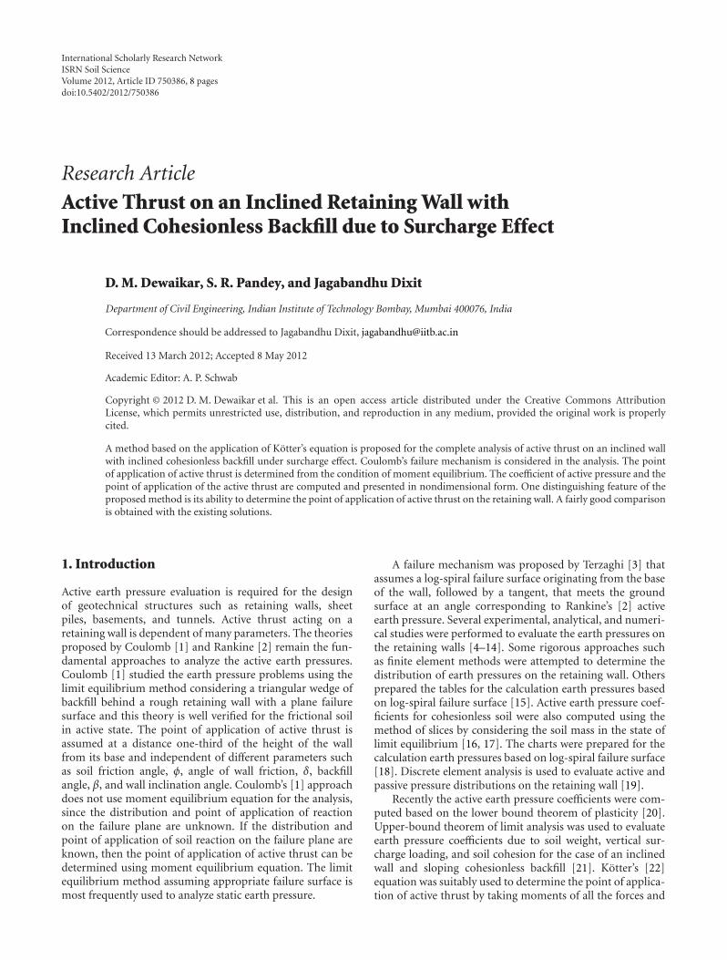
Figure 1: Free body diagram of the trial failure wedge ABC.

reaction about the base of the retaining wall [23]. A methodwas proposed by Kame et al. [24] to determine the activeearth pressure and its point of application on a vertical wallretaining horizontal cohesionless backfill based on log-spiralfailure mechanism coupled with Kotter’s equation. Dewaikaret al. [25] used Kotter’s equation to evaluate the magnitudeof active thrust on an inclined wall retaining horizontalcohesionless backfill with uniform surcharge and to find outthe point of application of reaction on the failure surface.

The objective of this study is to present a mathematicalapproach with a high degree of simplicity for the evaluationof the active thrust and its point of application. The analysisconsiders the free body diagram of the retaining wall in a verysimple and analytical procedure and is easier for engineeringapplication. The validity of the proposed approach is checkedwith previous available results.

2. Analysis of Active Thrust

The active thrust, Pa, is determined from the conditions offorce equilibrium and its point of application is determinedfrom the conditions of moment equilibrium. Figure 1 showsan inclined retaining wall, with inclined cohesionless backfillsubjected to a uniform surcharge intensity of q KN/m2.A trial plane failure surface [1] is considered which meetsthe ground surface at an angle, α with the horizontal. Thetrial wedge ABC is in equilibrium under the effect of threedifferent forces: (1) the equivalent force of the surcharge, W(2) the soil reaction, R along the face trial failure BC, at anangle φ to the normal on BC and (3) the active thrust Pa, atan angle δ to the normal on the back.

The symbols used in Figure 1 are defined as follows.

Pa: active thrust.

W : equivalent force of the surcharge.

R: soil reaction on the failure wedge.

H : height of the retaining wall.

h: height of point of application of active thrust fromthe wall base.

θ: inclination of the retaining wall with the horizon-tal.

δ: friction angle between the wall and soil backfill.

φ: soil friction angle.

α: inclination of the trial failure plane with thehorizontal.

q: intensity of surcharge in kN/m2.

Equating all the forces in the vertical and horizontaldirection, the following force equilibrium conditions areobtained.

Horizontal force equilibrium:

Pa sin(θ − δ) = R sin(α− φ

)(1)

from which R is obtained as

R = Pa sin(θ − δ)sin(α− φ

) . (2)

Vertical force equilibrium:

Pa cos(θ − δ) + R cos(α− φ

) = AC · q (3)

substituting the value of R from (2) into (3)

Pa cos(θ − δ) +Pa sin(θ − δ)sin(α− φ

) cos(α− φ

) = AC · q, (4)

Pa cos(θ − δ) + Pa sin(θ − δ)cot(α− φ

) = AC · q. (5)

From (5), Pa is obtained as

Pa = AC · qcos(θ − δ) +

[sin(θ − δ)cot

(α− φ

)] . (6)

Now, applying sine rule to the triangle CAN,

AC

sin(180− α)= AN

sin(α− β

) (7)

or

AC = AN · sin(180− α)sin(α− β

) . (8)

Referring to Figure 1,

AN = H(cot θ + cotα). (9)

Substituting the value of AN in (8), AC is obtained as,

AC = H(cotα + cot θ) sinα

sin(α− β

) . (10)

Substituting the value of AC in (6), the magnitude of activethrust Pa is expressed as

Pa = qH(cotα + cot θ) sinα

sin(α− β

)[cos(θ − δ) + sin(θ − δ)cot

(α− φ

)] . (11)

The maximum value of active thrust (Pa) is obtained whenthe inclination of the failure plane, BC, with the horizontalreaches the critical value, αcr.

ISRN Soil Science 3

Curvedfailure surface

Normal

Tangentdα

ds

dp

Slip

O

α

φ

Figure 2: Reactive pressure distribution along the failure surface.

3. Evaluation of Soil Reaction onthe Failure Surface

In a cohesionless soil medium with active state of equilibriumunder plane strain condition, Kotter’s [22] equation is givenas (Figure 2)

dp

ds− 2p tanφ

dα

ds= γ sin

(α− φ

)s, (12)

where

dp: differential reactive pressure at a point on thefailure surface,

ds: elemental length of the failure surface,

α: angle made by the tangent at the point of interestwith the horizontal,

φ: soil friction angle and,

γ: soil unit weight.

In the present analysis, only surcharge effect is takeninto consideration, and therefore γ becomes zero. With thisconsideration (12) can be written as

dp

dα= 2p tanφ (13)

or

dp = 2p tanφdα. (14)

For a plane failure surface, dα is zero and the correspondingsolution for the reactive pressure, p, is obtained as

p = constant. (15)

The above solution indicates that soil reactive pressure (p) isuniformly distributed along the failure plane, BC. Therefore,the resultant soil reaction, R, acts at the mid-point ofthe failure plane, BC. The magnitude of soil reaction iscomputed after knowing the critical value, αcr, of the angle,

hr

C

NM

A

R

Y

B

P

H

Q

W

X

90− θ

q (KN/m2)

φ

90−α

θ

β

δ

αcr

Pa

Figure 3: Free body diagram of the failure wedge ABC.

α. Substituting the value of Pa from (11) in to (2), the soilreaction R on the failure surface is obtained as

R = qH(cotαcr + cot θ) sin(θ − δ) sinαcr

sin(αcr − φ

)sin(αcr − β

)

× 1[cos(θ − δ) + sin(θ − δ)cot

(αcr − φ

)] .

(16)

4. Point of Application of the Active Thrust

After obtaining the value of Pa, the condition of momentequilibrium is applied. Figure 3 shows the free body diagramof the failure wedge ABC. The equivalent force of surchargeon the trial wedge, ABC, is AC ·q, which acts at the midpointof AC, that is, at a distance Y from the vertical line passingthrough the base the wall. As the distribution of reaction (R)is uniform along the failure surface, it acts at the mid-point ofthe failure plane BC. The moments of all forces and reactionsare taken about the base of the wall, at point B.

Moment equilibrium condition:

Pa cos δ · X + qAC · Y = R cosφBC

2. (17)

The surcharge acts at the center of AC with the distance Ygiven as,

Y = PQ cosβ, (18)

where

PQ = AC

2− AP. (19)

From triangle AMP,

AP = Hcot θcosβ

. (20)

Now, substituting the value of AC from (10) and AP from(20) in (19) (Figure 3), PQ is obtained as

PQ = H(cot θ + cotαcr) sinαcr

2 sin(αcr − β

) − Hcot θcosβ

. (21)

4 ISRN Soil Science

Table 1: Variation of the height of point of application of active thrust, Hr , with angle of wall back (θ), angle of soil friction (φ), soil andwall friction (δ) and backfill slope (β).

Angle of wall back, θ(degrees)

Angle of soil friction, φ(degrees)

Angle of wall friction, δ (degrees)(δ = 2/3φ)

Angle of backfill slope, β(degrees) β/φ = (0.4, 0.6, 0.8)

Hr (=h/H)

80

16 0.336

40 26.667 24 0.397

32 0.511

14 0.388

35 23.333 21 0.451

28 0.566

12 0.446

30 20 18 0.510

24 0.622

10 0.512

25 16.667 15 0.575

20 0.682

70

16 0.657

40 26.667 24 0.708

32 0.814

14 0.625

35 23.333 21 0.68

28 0.775

12 0.605

30 20 18 0.648

24 0.729

10 0.584

25 16.667 15 0.625

20 0.692

Substituting the value of PQ from (21) into (18), the point ofapplication of equivalent surcharge force from the axis BM(Figure 3) is computed as

Y = cosβ

[H(cot θ + cotαcr) sinαcr

2 sin(αcr − β

) − Hcot θcosβ

]

. (22)

The soil reaction R acts at the midpoint of the failure planeBC, with the distance, r (Figure 3), computed as

r = BC

2. (23)

Referring to Figure 3, BC is obtained as

BC = H sin(θ + β

)

sin(αcr − β

)sin θ

. (24)

Substituting the value of BC from (24) and Y from (22) into(17), the distance X is obtained:

Pa cos δ · X + q · AC cosβ

×[H(cot θ + cotαcr) sinαcr

2 sin(αcr − β

) − Hcot θcosβ

]

= R cosφH sin

(θ + β

)

2 sin(αcr − β

)sin θ

(25)

or

X =R cosφ

H sin(θ + β

)

2 sin(αcr − β

)sin θ

Pa cos δ

−q · AC cosβ

[H(cot θ + cotαcr) sinαcr

2 sin(αcr − β

) − Hcot θcosβ

]

Pa cos δ.

(26)

The height, h, of point of application of Pa from the wall baseis obtained as

h = X sin θ. (27)

The coefficient of active earth pressure (Kaq) for the retainingwall with the surcharge effect is obtained as

Kaq = Pa/γH. (28)

5. Results and Discussions

One of the aims of the proposed analysis is the determi-nation of point of application of the active thrust in anondimensional form with the consideration of effect of

ISRN Soil Science 5

70 72 74 76 78 80 82 84 86 88 90

Angle of wall back, θ

Hr

0.5

0.45

0.55

0.6

0.65

0.7

0.75

0.8

0.85

0.9

δ = 2/3φβ = 0.8φ

φ = 40◦φ = 35◦

φ = 30◦φ = 25◦

Figure 4: Variation of Hr with angle of wall back, θ, for β = 0.8φ.

0.45

0.5

0.55

0.6

0.65

0.7

0.75

δ = 2/3φβ = 0.6φ

70 72 74 76 78 80 82 84 86 88 90

Angle of wall back, θ

Hr

φ = 40◦φ = 35◦

φ = 30◦φ = 25◦

Figure 5: Variation of Hr with angle of wall back, θ, for β = 0.6φ.

5 6 7 8 9 10 11 12 13 14 15

0.570.580.59

0.60.610.620.630.640.650.660.67

φ = 40◦

θ = 65◦

Angle of backfill slope, β

Hr

δ = 2/3φ

φ = 35◦φ = 30◦φ = 25◦

Figure 6: Variation of Hr with angle of backfill slope, β, for θ = 65◦.

various parameters. The height, h, of point of applicationof the active thrust due to surcharge effect is expressed in anondimensional form, Hr , expressed as h/H . The results arereported as shown in Table 1 along with figures that aredescribed below.

0.54

0.56

0.58

0.6

0.62

0.64

0.66

Hr

θ = 70◦δ = 2/3φ

5 6 7 8 9 10 11 12 13 14 15

φ = 40◦


φ = 35◦φ = 30◦φ = 25◦


0.53

0.54

0.55

0.56

0.57

0.58

0.59

0.6

0.61

0.62

Hr

θ = 75◦δ = 2/3φ

5 6 7 8 9 10 11 12 13 14 15

φ = 40◦


φ = 35◦φ = 30◦φ = 25◦


In Figures 4 and 5, variation of Hr with the angle of wallback, θ, is shown for δ = 2/3φ and β = 0.8φ and 0.6φ respec-tively. It is seen that Hr , decreases with increasing angle ofwall back and increases with increasing soil friction angle, φ.

In Figures 6, 7, and 8, variation of Hr with the angle ofbackfill slope, β, with δ = 2/3φ is shown for θ = 65◦, 70◦, and75◦, respectively. It is seen that Hr , increases with increasingβ, with higher values for higher soil friction angle, φ.

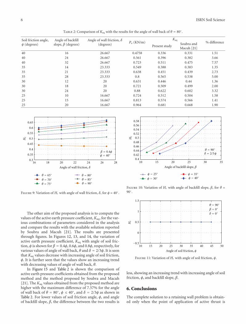
In Figure 9, variation of Hr with the angle of wall friction,δ, is shown for β = 16◦ and φ = 40◦. It is seen that Hr

increases with δ, with higher values for higher β.In Figure 10 is shown the variation of Hr for a vertical

wall (θ = 90◦) and δ = 2/3φ. It is again seen that Hr increaseswith increase of β.

In Figure 11, variation of Hr with angle of soil friction,φ, is shown for a retaining wall with angle of wall back, θ =90◦, backfill slope, β = 0◦, and angle of wall friction, δ = 0◦.It is interesting to note that Hr is a constant value of 0.5for all values of angle of soil friction, φ. Hence, the pointof application of active thrust acts at the mid-height of asmooth vertical retaining wall with horizontal backfill.

6 ISRN Soil Science

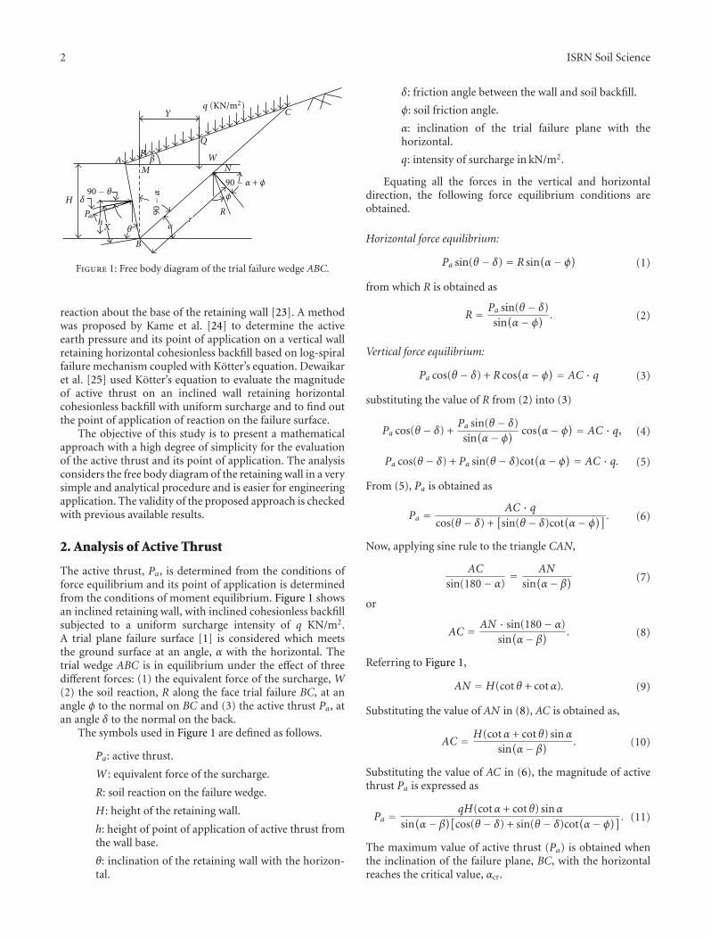
Table 2: Comparison of Kaq with the results for the angle of wall back of θ = 80◦.

Soil friction angle,φ (degrees)

Angle of backfillslope, β (degrees)

Angle of wall friction, δ(degrees)

Pa (KN/m)Kaq

% differencePresent study

Soubra andMacuh [21]

40 16 26.667 0.4758 0.336 0.331 1.5140 24 26.667 0.561 0.396 0.382 3.6640 32 26.667 0.723 0.511 0.475 7.5735 14 23.333 0.549 0.388 0.383 1.3535 21 23.333 0.638 0.451 0.439 2.7335 28 23.333 0.8 0.565 0.538 5.0030 12 20 0.631 0.446 0.44 1.3630 18 20 0.721 0.509 0.499 2.0030 24 20 0.88 0.622 0.602 3.3225 10 16.667 0.724 0.512 0.504 1.5825 15 16.667 0.813 0.574 0.566 1.4125 20 16.667 0.964 0.681 0.668 1.90

16 18 20 22 24 26 280.3

0.35

0.4

0.45

0.5

0.55

0.6

0.65

θ = 65◦

θ = 70◦

θ = 75◦

θ = 80◦

θ = 85◦θ = 90◦

β = 0.4φφ = 40◦

Angle of wall friction, δ

Hr

Figure 9: Variation of Hr with angle of wall friction, δ, for φ = 40◦.

The other aim of the proposed analysis is to compute thevalues of the active earth pressure coefficient, Kaq, for the var-ious combinations of parameters considered in the analysisand compare the results with the available solution reportedby Soubra and Macuh [21]. The results are presentedthrough figures. In Figures 12, 13, and 14, the variation ofactive earth pressure coefficient, Kaq with angle of soil fric-tion, φ is shown for β = 0.4φ, 0.6φ, and 0.8φ, respectively, forvarious values of angle of wall back, θ and δ = 2/3φ. It is seenthat Kaq values decrease with increasing angle of soil friction,φ. It is further seen that the values show an increasing trendwith decreasing values of angle of wall back, θ.

In Figure 15 and Table 2 is shown the comparison ofactive earth pressure coefficients obtained from the proposedmethod and the method proposed by Soubra and Macuh[21]. The Kaq values obtained from the proposed method arehigher with the maximum difference of 7.57% for the angleof wall back of θ = 80◦, φ ≤ 40◦, and δ = 2/3φ as shown inTable 2. For lower values of soil friction angle, φ, and angleof backfill slope, β, the difference between the two results is

10 15 20 25 30 350.4

0.420.440.460.48

0.50.520.540.560.58

φ = 40◦φ = 35◦

φ = 30◦φ = 25◦


θ = 90◦δ = 2/3φ

Hr

Figure 10: Variation of Hr with angle of backfill slope, β, for θ =90◦.

10 15 20 25 30 35 40 45 50

0

0.5

1

1.5

Angle of soil friction, φ

θ = 90◦

β = 0◦

δ = 0◦

Hr

−0.5

Figure 11: Variation of Hr with angle of soil friction, φ.

less, showing an increasing trend with increasing angle of soilfriction, φ, and backfill slope, β.

6. Conclusions

The complete solution to a retaining wall problem is obtain-ed only when the point of application of active thrust is

ISRN Soil Science 7

25 30 35 400

0.10.20.30.40.50.60.70.80.9

1

θ = 85◦

θ = 80◦

θ = 75◦

θ = 70◦

θ = 65◦


Kaq

δ = 2/3φβ = 0.4φ

Figure 12: Variation of Kaq with angle of soil friction, φ, for β =0.4φ.

θ = 85◦

θ = 80◦

θ = 75◦

θ = 70◦

θ = 65◦

δ = 2/3φβ = 0.6φ

25 30 35 400

0.10.20.30.40.50.60.70.80.9

1


Kaq

Figure 13: Variation of Kaq with angle of soil friction, φ, for β =0.6φ.

δ = 2/3φβ = 0.8φ

θ = 85◦

θ = 80◦

θ = 75◦

θ = 70◦

θ = 65◦

25 30 35 400.4

0.5

0.6

0.7

0.8

0.9

1


Kaq

Figure 14: Variation of Kaq with angle of soil friction,φ, for β =0.8φ.

10 15 20 25 30 35

0.35

0.4

0.45

0.5

0.55

0.6

0.65

0.7

θ = 80◦

φ = 40◦ present studyφ = 40◦ Soubra and Macuh [21]φ = 35◦ present studyφ = 35◦ Soubra and Macuh [21]φ = 30◦ present studyφ = 30◦ Soubra and Macuh [21]φ = 25◦ present studyφ = 25◦ Soubra and Macuh [21]


Kaq

Figure 15: Comparison of variation of Kaq with angle of backfillslope, β, evaluated in present study with filed results.

known. Kotter’s [22] equation lends itself as a powerfultool in the proposed analysis to determine the reactivepressure distribution on the failure plane. The momentequilibrium condition is used effectively to compute thepoint of application of the active thrust. From the proposedanalysis it is seen that the point of application of the activethrust depends upon a number of factors such as angle ofsoil friction, φ, angle of wall friction, δ, angle of wall back, θ,and inclination of backfill, β. It shows a wide variation in therange, 0.427 to 0.814. Only for the case of a smooth verticalwall retaining horizontal backfill, the point of applicationof the active thrust is at the wall mid-height. The presentapproach is easy to adapt for retaining walls and the resultsobtained based on this analysis are in fairly good agreementwith other results.

References

[1] C. A. Coulomb, “Essaisurune application des regles des max-imis et minimis a quelquesproblemes de statiquerelatifs al’architecture,” Memoires de Mathematiques et de Physique Pre-sentes a l’Academie Royale des Sciences par Divers Savants, vol.7, pp. 343–382, 1776.

[2] W. J. M. Rankine, “On the stability of loose earth,” Philosophi-cal Transactions of the Royal Society, vol. 147, 1857.

[3] K. Terzaghi, Theoretical Soil Mechanics, John Wiley & Sons,New York, NY, USA, 1943.

[4] J. B. Hansen, Earth Pressure Calculation, Danish GeotechnicalPress, Copenhagen, Denmark, 1953.

[5] V. V. Sokolovski, Statics of Soil Media, Butterworth, London,UK, 1960.

[6] Z. V. Tsagareli, “Experimental investigation of the pressure of aloose medium on retaining walls with a vertical back face andhorizontal backfill surface,” Soil Mechanics and FoundationEngineering, vol. 2, no. 4, pp. 197–200, 1967.

8 ISRN Soil Science

[7] M. Matsuo, S. Kenmochi, and H. Yagi, “Experimental study onearth pressure of retaining wall by field tests,” Soils and Foun-dations, vol. 18, no. 3, pp. 27–41, 1978.

[8] K. Habibagahi and A. Ghahramani, “Zero extension line the-ory of earth pressure,” Journal of the Geotechnical EngineeringDivision, vol. 105, no. 14702, pp. 881–896, 1979.

[9] Y. S. Fang and I. Ishibashi, “Static earth pressures with variouswall movements,” Journal of Geotechnical Engineering, vol. 112,no. 3, pp. 317–333, 1986.

[10] D. M. Potts and A. B. Fourie, “A numerical study of the effectsof wall deformation on earth pressures,” International Journalfor Numerical & Analytical Methods in Geomechanics, vol. 10,no. 4, pp. 383–405, 1986.

[11] E. Motta, “Generalized Coulomb active earth pressure for adistanced surcharge,” Journal of Geotechnical Engineering, vol.120, no. 6, pp. 1072–1079, 1994.

[12] H. Hazarika and H. Matsuzawa, “Wall displacement modesdependent active earth pressure analyses using smeared shearband method with two bands,” Computers and Geotechnics,vol. 19, no. 3, pp. 193–219, 1996.

[13] V. R. Greco, “Active earth thrust by backfills subject to a linesurchange,” Canadian Geotechnical Journal, vol. 42, no. 5, pp.1255–1263, 2005.

[14] Y. M. Cheng, Y. Y. Hu, and W. B. Wei, “General axisymmetricactive earth pressure by method of characteristics—theory andnumerical formulation,” International Journal of Geomechan-ics, vol. 7, no. 1, pp. 1–15, 2007.

[15] A. I. Caquot and J. Kerisel, Tables for the Calculation of PassivePressure, Active Pressure, and Bearing Capacity of Foundations,Gauthier-Villars, Paris, France, 1948.

[16] N. Janbu, “Earth pressure and bearing capacity calculationsby generalized procedure of slices,” in Proceedings of the 4thInternational Conference on Soil Mechanics and FoundationEngineering, vol. 2, pp. 207–212, London, UK, 1957.

[17] H. Rahardjo and D. G. Fredlund, “General limit equilibriummethod for lateral earth force,” Canadian Geotechnical Journal,vol. 21, no. 1, pp. 166–175, 1984.

[18] J. Kerisel and E. Absi, Active and Passive Earth Pressure Tables,Balkema, Rotterdam, The Netherlands, 1990.

[19] C. S. Chang and S. J. Chao, “Discrete element analysis foractive and passive pressure distribution on retaining wall,”Computers and Geotechnics, vol. 16, no. 4, pp. 291–310, 1994.

[20] R. Lancellotta, “Analytical solution of passive earth pressure,”Geotechnique, vol. 52, no. 8, pp. 617–619, 2002.

[21] A. H. Soubra and B. Macuh, “Active and passive earth pressurecoefficients by a kinematical approach,” Proceedings of theInstitution of Civil Engineers, vol. 155, no. 2, pp. 119–131, 2002.

[22] F. Kotter, Die Bestimmung des Drucks an gekrummten Gleitfla-chen, eine Aufgabe aus der Lehre vom Erddruck, Sitzungsberich-te der Akademie der Wissenschaften, Berlin, Germany, 1903.

[23] D. M. Dewaikar and S. A. Halkude, “Seismic passive/activethrust on retaining wall-point of application,” Soils and Foun-dations, vol. 42, no. 1, pp. 9–15, 2002.

[24] G. S. Kame, D. M. Dewaikar, and D. Choudhury, “Activethrust on a vertical retaining wall with cohesionless backfill,”Electronic Journal of Geotechnical Engineering, vol. 15, pp.1848–1863, 2010.

[25] D. M. Dewaikar, S. R. Pandey, and J. Dixit, “Active earth pres-sure on an inclined wall with horizontal cohesionless backfilldue to surcharge effect,” Electronic Journal of GeotechnicalEngineering, vol. 17, pp. 811–824, 2012.

Submit your manuscripts athttp://www.hindawi.com

Forestry ResearchInternational Journal of

Hindawi Publishing Corporationhttp://www.hindawi.com Volume 2014

Environmental and Public Health

Journal of



EcosystemsJournal of

Meteorology


Advances in

EcologyInternational Journal of


Marine BiologyJournal of


Hindawi Publishing Corporationhttp://www.hindawi.com

Applied &EnvironmentalSoil Science

Volume 2014

Advances in


Environmental Chemistry

Atmospheric SciencesInternational Journal of



Waste ManagementJournal of

Hindawi Publishing Corporation http://www.hindawi.com Volume 2014

International Journal of

Geophysics


Volume 2014

Geological ResearchJournal of

EarthquakesJournal of



Volume 2014

BiodiversityInternational Journal of

ScientificaHindawi Publishing Corporationhttp://www.hindawi.com Volume 2014

OceanographyInternational Journal of


The Scientific World JournalHindawi Publishing Corporation http://www.hindawi.com Volume 2014

Journal of Computational Environmental SciencesHindawi Publishing Corporationhttp://www.hindawi.com Volume 2014


ClimatologyJournal of

Documents

ActiveThrustonanInclinedRetainingWallwith ...downloads.hindawi.com/archive/2012/750386.pdf · Active earth pressure ... prepared the tables for the calculation earth ... Discrete