Enhanced Multicarrier Techniques for Professional Ad … fileTable of Contents 1 ... 2.3.2 Calculation of the timeout rate and delay in discrete time intervals ..... 9 2.4

ICT 318362 EMPhAtiC Date: 28/01/2015

ICT-EMPhAtiC Deliverable D5.3 1/42

Enhanced Multicarrier Techniques for Professional Ad‐Hoc and Cell‐Based Communications

(EMPhAtiC)

Document Number D5.3

Cross‐layer optimization of RRM with Physical and Application layers in PMR networks

Contractual date of delivery to the CEC: 31 December 2014

Actual date of delivery to the CEC: 28 January 2015

Project Number and Acronym: 318362 EMPhAtiC

Editor: Stephan Pfletschinger (CTTC)

Authors: Dimitris Tsolkas (CTI),

Marius Caus (CTTC)

Yao Cheng (ITU), Martin Haardt (ITU),

Antonio Cipriano (TCS), Luxmiram Vijayandran (TCS),

Mylene Pischella (CNAM)

Participants: CTI, CNAM, TCS, CTTC, ITU

Workpackage: WP5

Security: Public (PU)

Nature: Report

Version: 1.1

Total Number of Pages: 42

Abstract:

This report presents new progress on cross‐layer techniques and Radio Resource Management (RRM) algorithms for broadband PMR networks. Cross‐layer adaptation in cell‐based PMR communications is first investigated, and a cross‐layer scheme is devised to offer an increased number of PMR connections with satisfactory Quality of Experience (QoE), which is crucial in crisis scenarios. Taking into account the inter‐cluster interference, an enhanced version of the Distributed bUffer Stabilization RRM algorithm (DUST) is proposed for PMR networks. In addition, with a focus on multi‐user MISO downlink scenarios, an efficient margin adaptive scheduling algorithm is tailored for FBMC, contributing to a solution to the challenging joint design of transmit and receive processing, the channel assignment as well as the power allocation.

Ref. Ares(2015)355345 - 29/01/2015



Table of Contents

1. Introduction ................................................................................................. 3 2. Increasing PMR capacity through encoding rate adaptation.......................... 4

2.1 Adopted PMR scenario .................................................................................. 4 2.2 The Proposed cross-layer scheme .................................................................. 5 2.3 Theoretic analysis using Continuous Flow Modelling .......................................... 6

2.3.1 General Continuous Flow Model ............................................................... 6 2.3.2 Calculation of the timeout rate and delay in discrete time intervals ............... 9

2.4 Derivation of the optimal adaptation thresholds ............................................. 10 2.4.1 Objective estimation of QoE .................................................................. 10 2.4.2 Thresholds calculation .......................................................................... 12

2.5 Performance evaluation .............................................................................. 13 3. Evolution of DUST algorithm using interference information ....................... 16

3.1 Evolution compared to D5.2 ........................................................................ 16 3.2 Algorithm description ................................................................................. 18 3.3 Numerical Experiments .............................................................................. 22 3.4 Performance summary ............................................................................... 29

4. Scheduling algorithms for FBMC systems ................................................... 30 4.1 Introduction ............................................................................................. 30 4.2 System model ........................................................................................... 30 4.3 SDMA with block diagonalization .................................................................. 31 4.4 Margin adaptive scheduling algorithm ........................................................... 32 4.5 Successive channel allocation ...................................................................... 34 4.6 Numerical results ...................................................................................... 36 4.7 Conclusions .............................................................................................. 38

5. Conclusions ................................................................................................ 39 6. References ................................................................................................. 40



1. Introduction

This report considers cross‐layer techniques for the optimization of Radio Resource Management (RRM) algorithms in PMR networks and places special emphasis on the interactions between the physical and the application layers. Techniques and results on cross‐layer RRM for multiple clusters which have been reported in deliverable D5.2 have been extended to consider cross‐cluster interference.

The first section considers cross‐layer adaptation in cell‐based PMR communications: The interplay between the source coding of critical voice communication, which is located in the application layer, and the number of simultaneous calls which can be accommodated by the system is investigated and an algorithm inspired by the design principle continuous flow modelling has been developed.

Section 3 investigates RRM for multiple clusters considering Cyclic Prefix Orthogonal Frequency Division Multiplex (CP‐OFDM), filter bank multicarrier (FBMC) and perfect modulation (PM), which is an idealized modulation that does not cause adjacent interference. The design objective is a stable queue for all users and the minimization of the energy consumption taking into account non‐negligible inter‐cluster interference. An extension of the backpressure algorithm is developed and the achieved performance is evaluated for different scenarios, in particular the differences between OFDM and FBMC are assessed. Signalling between different clusters for interference coordination has been considered.

The last section addresses the Multi‐User Single Input Multiple Output (SU‐SIMO) margin adaptive problem for the FBMC modulation based on the offset QAM (OQAM), referred to as FBMC. The analysis conducted in that section reveals that due to the specific FBMC transmission format the system has to deal with inter‐user, inter‐symbol and inter‐carrier interference to solve the resource allocation problem. To manage the interference, the successive channel allocation method, originally proposed for the CP‐OFDM, has been modified by organizing subcarriers in groups and assigning subcarriers to users in a block‐wise fashion. Following this strategy and making some approximations we demonstrate that it is possible to pose a single problem that is valid for OFDM and FBMC. In this case, numerical results show that FBMC is more energy‐efficient than OFDM because it requires less power to transmit the same information rate.



2. Increasing PMR capacity through encoding rate adaptation

2.1 Adopted PMR scenario

The adopted scenario refers to cell‐based PMR communications, where in each cell, time and frequency synchronized transmissions (including potentially direct transmissions through Direct Mode Operation ‐ DMO) take place under the control of a base station (BS). It is assumed that network dimensioning/planning procedures have taken place, while the BSs are inter‐connected through a backbone infrastructure. The Hand Helds (HHs) and the Mobile Stations (MS) are randomly deployed in each cell, while the transmissions of a dynamic set of HHs/MSs may be critical referring to communications for Public Protection and Disaster Relief (PPDR).

This scenario may model situations such as a car accident, train crash, traffic jam, an earthquake event etc., where coordination among police officers/firemen is needed at a specific area inside a cell while all citizens try to communicate especially the first moments after the event (Fig. 2‐1). Practically, in such situations specific set of HHs/MSs (e.g., HHs of police officers) requires scheduling priority, since their transmissions carry vital information. The BSs must serve the critical traffic with priority and guarantee the quality requirements of the non‐critical traffic as well. An efficient way to deal with this problem has been proposed in D5.2 [1], where an enhanced proportional fair RRM algorithm has been proposed. However, in such critical scenarios, even if the critical traffic is served with priority, it increases rapidly requiring solutions for improving the capacity of the critical traffic. To this end, here we focus on critical voice connections and propose a cross‐layer mechanism for optimizing RRM by adjusting the encoding rate in application layer. The proposed optimization targets at maximizing the active HHs in the system, with the cost of a controlled degradation on end users’ quality of experience (QoE).

Figure 2-1: Illustration of the cell-based PMR scenario



2.2 The Proposed cross‐layer scheme

The proposed cross‐layer scheme is split into two parts, namely the BS part and the HH part, residing at the BS and each HH, respectively (Fig. 2‐2). Regarding the first part, the BS starts by collecting all the required information regarding the performance status of each one of its active connections. Subsequently, the BS uses the collected information to run a decision algorithm for adjusting the encoding mode in application layer. This decision is taken separately by the HH part after BS’s order and aims at counterbalancing the number of PMR voice connections in the system and the achievable QoE at HHs. This is a critical issue in crisis scenarios, since the establishment of a voice connection is of high importance, while the achievable QoE level can be more relaxed. Our main focus is on proposing a cross layer decision algorithm for the BS part. This algorithm takes into account the packet timeout rate and the mean delay of each connection and decides on the adaptation of media encoding rates towards an increased number of PMR connections with acceptable QoE in the system.

Figure 2-2: The proposed cross layer scheme

Assume active PMR connections in a cell, the parameters that are used by the decision algorithm are the following:

, is the packet timeout rate of the connection, i.e., the percentage of

packets that were lost due to deadline expiration (packet delay has exceeded maximum acceptable delay).

is the mean delay of the connection.

, is the encoding mode (of the available modes) for the connection,

1,2, . . . .

, , , are the maximum tolerable timeout rate and maximum acceptable delay

of the connection, respectively,



is a threshold indicating a very low delay ratio: (,).

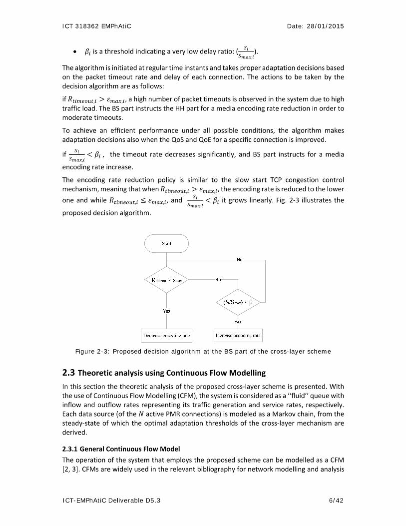
The algorithm is initiated at regular time instants and takes proper adaptation decisions based on the packet timeout rate and delay of each connection. The actions to be taken by the decision algorithm are as follows:

if , , , a high number of packet timeouts is observed in the system due to high traffic load. The BS part instructs the HH part for a media encoding rate reduction in order to moderate timeouts.

To achieve an efficient performance under all possible conditions, the algorithm makes adaptation decisions also when the QoS and QoE for a specific connection is improved.

if ,

, the timeout rate decreases significantly, and BS part instructs for a media

encoding rate increase.

The encoding rate reduction policy is similar to the slow start TCP congestion control mechanism, meaning that when , , , the encoding rate is reduced to the lower

one and while , , , and ,

it grows linearly. Fig. 2‐3 illustrates the

proposed decision algorithm.

Figure 2-3: Proposed decision algorithm at the BS part of the cross-layer scheme

2.3 Theoretic analysis using Continuous Flow Modelling

In this section the theoretic analysis of the proposed cross‐layer scheme is presented. With the use of Continuous Flow Modelling (CFM), the system is considered as a ‘‘fluid’’ queue with inflow and outflow rates representing its traffic generation and service rates, respectively. Each data source (of the active PMR connections) is modeled as a Markov chain, from the steady‐state of which the optimal adaptation thresholds of the cross‐layer mechanism are derived.

2.3.1 General Continuous Flow Model

The operation of the system that employs the proposed scheme can be modelled as a CFM [2, 3]. CFMs are widely used in the relevant bibliography for network modelling and analysis



[4–6]. CFM representation of communication networks’ traffic and elements is justified from the fact that in a high‐speed packet switching network a packet may be considered as a water molecule with a virtually infinitesimal effect on the entire flow. Thus, the adoption of a CFM can significantly reduce the complexity of the representation of the system that employs the proposed scheme, as compared to a standard representation at packet level. The CFM used here consists of a ‘‘fluid’’ queue whose inflow and outflow processes are characterized by flow rates, while its content is defined by the volume of the stored fluid. The size of the queue is finite. Thus, in case the queue is full, the excess flow cannot be absorbed, leading to overflow. The basic storage unit of this model is a symbol. Assume that the active PMR connections in a cell are identical and each one is fed by a data source producing a continuous data flow with maximum tolerable delay . The basic parameters of the CFM are the following:

1. inflow rate in symbols/second 2. Constant service rate in symbols/s (the PHY layer time frame is considered to

have a duration of seconds and serve symbols).

3. ∙ Queue size in symbols. Its value is such that overflow occurs when the

delay of a queued symbol exceeds the maximum tolerable value . 4. : Queue load in symbols. 5. : Outflow rate in symbols/second. 6. : Overflow rate in symbols/second.

Let us define for each data flow: a variable encoding rate equal to , bits/second where

1,2, … and is the number of discrete encoding modes, and a modulation order bits/symbol. The inflow rate of each source is:

, , while the total inflow rate:

∑ (2.1)

The buffer load is described by the differential equation:

0, 0

0,

,

(2.2)

The total outflow rate is defined as:

, 0

, 0 (2.3)

The total overflow rate is defined as:

,

0, 0 (2.4)

The overflow rate of each source is proportional to the percentage of the source inflow rate with respect to the total system inflow rate.



∙ (2.5)

where

∑ (2.6)

The total overflow volume during the time interval 0, is defined as follows:

(2.7)

while the overflow of the data source is

(2.8)

Thus, the total overflow rate during the time interval 0, is

(2.9)

while the overflow rate of the source is

, (2.10)

This corresponds to the connection packet timeout rate , , which is the key value used in the proposed decision algorithm.

The data successfully served by the queue (i.e., scheduled for transmission) are transmitted over the wireless medium. The data loss due to channel conditions of the connection is as follows:

∙ 1 1 (2.11)

where is the BER for the connection. Consequently, the total loss due to the wireless channel is:

∑ (2.12)

During the time interval 0, is:

(2.13)

And, thus, the total loss rate due to the wireless channel is

(2.14)

Finally, the total loss rate due to timeouts (overflow) and the wireless channel is

∙ 1 (2.15)



The proposed algorithm changes its decision in specific time intervals. The BS monitors the network for a period of time (a number of subframes) and then decides on changing or not the encoding rate. To this end, next we provide the calculation of the loss rate and the delay in discrete time intervals.

2.3.2 Calculation of the timeout rate and delay in discrete time intervals

Let us consider a system that consists of a single data source, the fluid queue and the wireless medium. The source generates data with an encoding rate , bits/s, where

1,2,… . It is assumed that during the observation interval 0, the functions and are piecewise constant with a finite number of ‘‘jumps’’. In this case, the function

is piecewise linear, while the functions and are piecewise constant as well. The decision algorithm has to determine the appropriate values of , , thus to adapt the value of every seconds (where Δ is a constant). If the quality of the wireless channel is assumed to be constant during a time frame, then 0, . Thus, the 0, interval is

divided into subintervals of seconds: , , where 0 and , during

each of which the value of the function is constant. The value of is by definition constant during all these time intervals.

2.3.2.1 Calculation of the timeout rate

Let , , be the values of , , , respectively, during the time interval

, . Similarly, is the buffer load at , and is the

overflow volume during , .

The buffer load at is: minmax ∙ , 0}, C}, while the overflow

volume during , , is ,

0, .

Thus, the overflow rate is:

, ∙ (2.16)

Additionally the loss rate due to the wireless channel is:

, 1 1 (2.17)

Consequently,

, , , ∙ 1 , (2.18)

2.3.2.2 Calculation of the mean delay

The value of the data source mean delay, , during , is derived from the mean buffer load (given the constant service rate of the queue). More specifically, in the time interval

, the mean buffer load is:



(2.19)

Thus, for the mean delay we have:

∙ (2.20)

2.4 Derivation of the optimal adaptation thresholds

Voice is one of the dominant services in crisis scenarios. Taking this into account the main target of the proposed scheme is to adapt the voice encoding rate of HHs at application layer under controlled degradation at the end‐user’s QoE. QoE is a strongly subjective term and also one of the dominant factors for assessing a provided service. The most common measure of the QoE is the Mean Opinion Score (MOS) scale recommended in [7]. The MOS ranges from 1 to 5, with 5 representing the best quality, and is commonly produced by averaging the results of a subjective test, where end‐users are called under a controlled environment to rate their experience with a provided service. However, the subjective methodologies (e.g., use of questionnaires) are cost‐demanding and practically inapplicable for real‐time monitoring of the service performance.

2.4.1 Objective estimation of QoE

Different objective methods have been proposed to measure the speech quality. These methods can be classified into intrusive and non‐intrusive methods. Intrusive methods, such as the Perceptual Speech Quality Measure (PSQM) and the PESQ (Perceptual Evaluation of Speech Quality), estimate the distortion of a reference signal that travels through a network by mapping the quality deterioration of the received signal to MOS values. However, the need for a reference signal is a drawback for using intrusive methods for QoE monitoring. To this end, non‐intrusive methods have been defined such as the E‐model and the ITU P.563 [8]. Since the ITU P.563 method has increased computational requirements, making it inappropriate for monitoring in real‐time basis, we adopt the easier to be applied E‐model, described in the next section.

2.4.1.1 The E‐model

The E‐model [9] has been proposed by the ITU‐T for measuring objectively the MOS of voice communications. It is a parametric model that takes into account a variety of transmission impairments producing the so‐called Transmission Rating factor factor) scaling from 0 (worst) to 100 (best). Then a mathematic formula is used to translate this to MOS values. In the case of the baseline scenario where no network or equipment impairments exist, the factor is given by:

93.2 (2.21)

However, delays and signal impairments are involved in a practical scenario and hence the factor is given by:

(2.22)

where:

: the impairments that are generated during the voice traveling,



: the delays introduced from end‐to‐end signal traveling,

: the impairments introduced by the equipment,

: allows for compensation of impairment factors when there are other advantages of access to the user (Advantage Factor). It describes the tolerance of a user due to a certain advantage that he/she enjoys, e.g., not paying for the service or being mobile. Typical value for cellular networks: 10.

Focusing on parameters which depend on the wireless part of the communication it holds that [10]:

0.024 0.11 177.3 177.3 (2.23)

where:

0, 01, 0

and is the average packet delivery delay composed by two parts, the scheduling delay, denoted by , plus the roundtrip delay, denoted by i.e., . Low delay values below 150ms have very little impact on call quality or interactivity. As delay values continue to increase above 150ms call quality further degrades, with delays above 400ms making a duplex call extremely difficult due to loss of interactivity. Regarding the proposed scheme the value for a connection corresponds to the value defined in the CFM description above.

Also, the packet loss rate, , affects the parameter as follows [11]:

95 ∙∙

∙ (2.24)

where is an encoding mode depended equipment impairment factor obtained from [12] and shown in Table 2‐1, is a codec specific loss robustness factor and is the quotient of the average burst length and is dependent upon the theoretical burst length under random loss conditions. Considering that a single frame is sent per packet giving independent losses we set = 1. For AMR has not been defined for all modes. However, it is dependent upon the inter‐packet dependencies and the packet loss concealment scheme, and so since all AMR codec modes have a similar structure we utilize the value defined for the 12.2kbps mode of 10 for all codec modes [12].

The factor can be transformed to MOS values to retrieve results comparable with results provided by subjective methods. The transformation formula is as follows:

1, 0,

1 0.035 60 100 ∙ 7 ∙ 10 , 0 100,4.5, 100.

(2.25)

The proposed scheme increases the PMR capacity in respect to a specific (or MOS) threshold, which represent the minimum acceptable QoE level for a PMR voice connection. Based on this threshold the , and thresholds are calculated as described in the next

subsection.

Table 2‐1: Encoding modes



Encoding Mode

Application layer Encoding Rate (Kbps)

1 12.2 5

2 10.2 9

3 7.95 15

4 7.4 16

5 6,7 20

6 5,9 23

7 5,15 27

8 4,75 29

2.4.2 Thresholds calculation

We first depict in Fig. 2‐4 the achievable MOS values for different , ,and delay values. For minimum acceptable MOS=3 and MOS=2.5, the threshold values that can be used by the proposed scheme are depicted in Fig. 2‐5, and Fig. 2‐6, respectively.

Fig. 2‐4: MOS for various delay and timeout rate values



Fig. 2‐5: Threshold values that can be used by the proposed scheme for minimum acceptable MOS=3

Fig. 2‐6: Threshold values that can be used by the proposed scheme for minimum acceptable MOS=2.5

2.5 Performance evaluation

We evaluated the proposed scheme when it is applied on top of OFDMA and FBMC PHY, using the parameters depicted in Table 2‐2. The adaptation decision is taken every 10ms, while the timeout and delay thresholds 0.05, 0.3, are used, respectively. Based on the analysis in previous subsection, these thresholds guarantees QoE of about MOS=2.5 for a



roundtrip delay 300ms. Since the proposed scheme is based on the timeout rate, meaning on the rate of packets that are not scheduled for transmission due to high traffic conditions, the key difference between the OFDMA and FBMC scenario lies on the channel service rate. Using the same bandwidth for both the scenarios, FBMC provides higher service rate due to the absence of CP, i.e., the same amount of data can be sent in shorter frame duration [20].

Table 2‐2: Evaluation parameters

Parameter value

Bandwidth 5MHz

frame duration 10ms (OFDMA) 9.33ms (FBMC)

Slots/subframe 2

Data Symbols/slot 7

Data Bits/Symbol 6

Number of RB 25

Data subcarriers/RB 12

Roundtrip delay 300ms

BER 10e‐7

Fig. 2‐7 depicts the timeout rate in the network when the proposed scheme is disabled (“No adaptation”) and enabled (“Proposed adaptation”) for both the OFDMA and FBMC cases. The first observation regarding Fig. 2‐7 is that for the conventional case, with no rate adaptation, the FBMC leads to about 14% more PMR capacity comparing to OFDMA scenario (FBMC can serve 126 HHs while OFDMA 110 HHs). By enabling the proposed scheme, the total gain for the FBMC and OFDMA scenario is 72% and 50%, respectively.

Fig. 2‐7: Comparison of the proposed scheme with the conventional scenario (no adaptation) for the OFDMA and FBMC cases

Here is the performance summary of the proposed cross‐layer scheme:



To involve application layer performance metrics in lower layer procedures, reliable monitoring of these metrics is required. In the case of the QoE metric, the E‐model provides an efficient and easy to apply formula, which can be exploited by the BS of the PMR network.

Application layer rate adaptation provides sufficient capacity gain for the critical transmissions in a PMR network, using as a criterion the end‐user’s QoE.

The performance of the proposed scheme has negligible variations for the different PHY schemes (OFDMA and FBMC), since it is based on scheduling and application layer procedures. Cross layer schemes that involve physical layer parameters, e.g., the SINR, are expected to lead to higher performance differentiations. Such a scheme is provided in the next section.



3. Evolution of DUST algorithm using interference information

This work is an evolution of the Distributed bUffer Stabilization RRM (DUST) algorithm described in D5.2, Section 7. In particular, the main objective is to address large inter‐cluster interference by taking advantage of the aggregate interference cross‐layer information I(t) obtained from the physical layer, assuming that it has sensing capability.

3.1 Evolution compared to D5.2

In D5.2, we addressed the resource allocation problem for an asynchronous clusterised PMR ad‐hoc network that uses the spectral gaps in between other existing communication networks, , as depicted in Figure 3‐1.

Figure 3-1: Clusterised network scenario

For such heterogeneous networks, besides the direct channel interference, the adjacent ones also need to be considered. As such, we considered both CP‐OFDM and FBMC modulations, as well as the so‐called Perfect modulation (i.e., no adjacent interference). We sought to stabilize each user data queue while minimizing their average transmission energy. In order to cope with the long term stochastic nature of the problem and the inter‐cluster interference in a distributed way an algorithm was proposed adapted from the centralized backpressure approach. It was shown that the algorithm allows to trade between energy efficiency and the buffer delay. Compared to the classical centralized backpressure approach [13], a special dynamic weight was introduced to balance the independent cluster traffic requirements (i.e.,



D5.2‐Eq. 7.7), such that the objective function to be maximized at every instance was given by, D5.2‐Eq 7.9, i.e., optimize to maximize

nMm

mnmmn tptttt )()()()()( (3‐1)

where is the set of all links affected to cluster , μ and are the theoretical

Shannon capacity and the transmit power, respectively, , and are dynamic variables controlled by the algorithm. The proposed algorithm was shown to perform well when the inter‐cluster interference is not high. However, when the inter‐cluster interference is high it may lead to destructive competition. In other words, if a given cluster does not succeed to get the desired throughput (thus steadily increasing data queue), it will keep on increasing its transmission power until reaching the maximum power. Then, links will most probably always interfere each other (especially those near the edge) without any of them achieving there desired rate. Thus, we propose to enhance the DUST algorithm even when the inter‐cluster interference can be high (depending also on the transmit power). To do so, we use a key statement that was proved in [14]. It is stated that when the cross‐interference is higher than some level, the optimal allocation is an FDMA‐type allocation. In other words, transmission should be separated by any mean (e.g., frequency or time, FDMA, TDMA) such that there is no interference among different clusters. “One intuitive way to impose orthogonal communications between independent clusters’ links is to randomly turn‐off some of the available Resource Blocks (RBs) for a random period of time”. The above intuition is the base line of the entire enhancement as compared to D5.2 Section 7. In the sequel, we refer this process of turning‐off the RBs as transmission back‐off algorithm. It is important to note that the selection of allowed RBs using the back‐off algorithm is done before the basic backpressure algorithm. The output of the back‐off algorithm is an entry for the main algorithm by providing the pre‐selected RBs for the RRM optimization. Of course, the main and difficult objective is to cleverly control the back‐off selection, in particular using side information. Here are some important desired and undesired features to consider:

As a Cluster Head (CH), turning‐off some RBs will allow links from other clusters to experience better SINR. The effect is reciprocal if other clusters follow the same policy and will be beneficial for him.

Clusters being selfish, back‐off is performed if it does not harm their own communication in the long‐run.

If the cluster is willing to back‐off, the time and the number of RBs for back‐off should depend on the relative ratio between the local throughput requirements and others requirements (which entails signalling).

As for the side‐information, we use two main assumptions. First, nodes are enhanced with sensing capability such that they can assess the level of aggregate interference introduced by other links from other clusters. The interference information from the physical layer is then provided to the MAC layer (i.e., cross‐layer information). Second, a unique control channel, limited in capacity, exists where any CH can listen or broadcast. This channel is used by the CHs to exchange the required signalling information in order to run the back‐off algorithm. Since in practice exchanges of signalling are limited and sensible to losses, we will also investigate the performance degradation when the probability of correctly receiving the broadcasts decreases.



Let us first resume the problem setting detailed in D5.2, Section 7. Consider an asynchronous clustered PMR scenario where the unique CH, elected in each cluster, is in charge to manage the local RRM and can broadcast limited signalling to all neighbour CHs using the limited common channel. The main objective is to minimize the nodes transmission energy while stabilizing their data buffer queue (i.e., for brevity, on the long term the data buffer remains within a constant level, assuming that the system is feasible). In particular, we seek to optimize the long term energy efficiency instead of the instantaneous power (see, D5.2). Assume clusters composed of total communication links that form an asynchronous clusterised ad‐hoc network. The entire frequency band is composed of resource blocks (RBs) representing the set . A cluster is associated with the sub‐set of allowed RBs ,

∈ . The transmitter of link has a data buffer whose dynamic is simply defined as

)()()1()( tattqtq

where q t represents the data buffer size, a is the stochastic random input bits, )(t is the

theoretical throughput, and )0,max(xx . Each CH asynchronously optimizes and updates

the allocation policy for all the internal links following some algorithm, e.g., DUST algorithm. The following assumptions are considered:

to ease the analysis, we assume a time‐slotted system (i.e., discrete time t, representing for example a milli‐second),

the capacity )(t of a given link m using the thk RB is defined by the basic Shannon

capacity ))()(

1(log)()(

0

)()(

2 km

kmm

km

Kkkm IN

tgtpBt

n

, where kB is the bandwidth of the thk

RB.

the intra‐cluster links allocations are assumed orthogonal, i.e., only one link can be scheduled in a given RB, such that there is no intra‐cluster interference. Furthermore, we also assume that adjacent channel interference within the same cluster is neglected (e.g., CP large enough with OFDM to account for the maximum delay inside the cluster, and using guard subcarriers with FBMC). However, since each asynchronous CH optimizes their RRM independently, inter‐clusters interference cannot be avoided for both the direct and the adjacent channels, which is the main difficulty for the distributed RRM.

intra‐cluster signalling between nodes and their CH is assumed perfect without losses,

whereas broadcast signalling is assumed sensible to collisions, e.g., SINR smaller than

some threshold.

the clustering of the links and the selection of the unique cluster head (CH) in each

cluster is not investigated here and is assumed to follow some clustering algorithm

(e.g., [17], [32]),

the pre‐allocation of the set for each cluster n is not addressed here

3.2 Algorithm description

We first describe the overall algorithm provided in Algorithm 1 with few modifications compared to the one described in D5.2.



The core of the optimization problem to be solved is given in line 5. Compared to the initial DUST algorithm described in D5.2, Section 7.5.1, where the objective was to maximize

nMm

mnmmn tptttt )()()()()( , we now discard the use of the parameters )()( tt nn

and the related time varying trade‐off parameter )(t . The main reason is that this approach

slowly balances the power transmission from one link to another one in a continuous motion. However, recall the key statement from [14] which says that when the cross‐talk interference (i.e., inter‐cluster interference) is important, the best allocation is an orthogonal one. Hence, this continuous balancing of power instead of an ON/OFF style allocation can yield important wastes. Thus, instead of this continuous power balancing approach thanks to the variation of parameters )()( tt nn and )(t , we decide to keep unchanged the basic centralized back‐

pressure approach (see e.g., [13] [15]) in each cluster, i.e., we simply maximize

nMm

mmm tpttq )()()( where the data queue level )(tq m.is the only weight for the

throughput and is a constant that does not vary along time However, we employ the idea of

RBs back‐off, which directly impacts the computation of

)(

)()(tKk

mm

n

tt , by restricting the

allowed set )(tK n. This restriction is crucial and is handled by the proposed back‐off

Algorithm 2, applied in line 5 of Algorithm 1. In order to run Algorithm 2, each local CH needs information about the other clusters, in our case through (as explained in more details

after Algorithm 1). Line 10 to 16 represents the preparation of that local information at each cluster before broadcasting, whereas Line 17 to 22 represent the update after successful or failed broadcast reception by the clusters receiving the broadcast.



Note that in line 6, when performing the optimization for the current asynchronous allocation, the interference is based on the previous time epoch, i.e., a CH cannot know the new allocation in advance. However, when computing the theoretical throughput in line 7, the interference is from the current time (to be recorded for the next time epoch optimization). Let us now focus on the back‐off algorithm. In order to decide how many random RBs are to be turned‐off as well as the random back‐off time, we define information, called

n that is to

be broadcasted by the thn CH. That information simply reflects the interfered links cumulated queue. Assume for example 3 links in a cluster with current buffer size, 1Kb, 2Kb, 5Kb, and such that only user 2 and 3 are interfered (e.g., because there are located at the cluster edge). Thus, CH n needs to broadcast 7n Kb, and all other CHs, record that information. However,

since broadcast can be lost, and all CHs may not correctly receive the broadcast, it is necessary that each CH maintains its own specific knowledge about others, (up‐to‐date, or not). Thus,



instead of a unique n known by all CHs, we define )(', t

nn as the information known by

cluster n about cluster 'n . Of course 'nn means the cluster’s local information which is

always assumed up‐to‐date (i.e., nnn , ).

To create

n at each CH, it is first important to define when a link is “considered as interfered

or not”. Following an intuitive (heuristic) approach, the interfered state is assumed as true for one of the following cases:

the average SINR is lower than some threshold . To compute the average SINR, we use the average non‐zero transmit power within the last

T epoch, and the

corresponding average channel strength and aggregate interference.

there is no transmission within T , and the average queue size within

T is larger than

some threshold.

The reason behind the first point is related to the fact that the decision whether or not a link

is in an interference state, is through the SINR and not only the interference )1( tIm itself.

Using a threshold directly on the interference is not meaningful without considering the level of the utile signal. Thus, we consider the past non‐null power to compute the average transmit power within

T . However, recall that the basic back‐pressure algorithm may decide to not

transmit when the interference of a given link is too high compared to the level of its queue, such that it may postpone for a long period before deciding to transmit. Therefore, we need to assume to be in interference state if there is no transmission for a period of time but having the mean queue larger than some value (i.e., second criteria). Of course

T should be selected

not too small. Assume for example a link with very low traffic requirement and good channels that do not often need to transmit but in burst. It would be wrong to assume that it is experiencing interference. We have just defined the information that is computed by each CH then broadcasted. Based

on '),(' ntnn , each cluster n then needs to decide how many random RBs will be turned‐

off and for how long. As, such we propose the following heuristic approach, with the following intuitive (heuristic) objectives.

the number of RBs to be turned off should be larger as the ratio between the number

of total interfered links, i.e., nn

n n'

)( ' , becomes larger than the internal cluster links

total queue plus nn

n n'

)( ' . This means that if a cluster n is experiencing lots of

interfered links, it will expects other clusters to apply some back‐offs. In the other

hand, if cluster n is informed that others are experiencing some bad interferences, it will apply some back offs. . Note that the choice of the ratio threshold, ζ1 should be related to the system, e.g., to the number of clusters (or estimation).

the clusters being selfish, most probable in practice, the back‐off would be accepted only under certain conditions e.g., cluster n does not experience too much delay in helping others,

the RBs to be turned‐off by cluster n is randomly selected among nK ,



the time for back‐off is randomly selected, given a maximum time,

since each cluster optimize its RRM based on the previous interference state, doing a back‐off for only 1 time cannot be useful for others (otherwise when the other CH decides to transmit believing there is no interference, the local cluster would already start again to transmit, thus interfering). Thus, back‐off should be activated if and only if the time for back‐off is at least equal to 2 and the number of RBs to be turned off is at least equal to 1.

Based on the intuitive objectives described above, the detailed algorithm for the back‐off is described hereafter.

3.3 Numerical Experiments

The performance of the Algorithm 1 is demonstrated using the static spatial setting depicted in the following Figure 3‐2.



Figure 3-2: Simulation scenario: 4 squared-clusters with cluster center represented by the cross; 3 random links per cluster; each cluster uses one of the 2 sets of RBs (pink or

green) with 3RBs in each set.

There are 4 clusters (N 4) and 3 random links in each cluster (M 12). The size of the square‐clusters is 1 km wide. It is interesting to assess the algorithm for two main different situations, low and high inter‐cluster interference. To do so we use two different spreadings of the 4 clusters by varying in Figure 3‐2 such that d 2 km and d 100 m to model low and high inter‐cell interference, respectively. Note that, as opposed to D5.2, we do not use the ITU model with 9dB shadowing, in order to easily assess the relation between the different observed performances and the spatial static setting. Thus, the channel gains are obtained using only d . The noise level is defined by 174 dBm/Hz, and P_max=30 dBm (note that in [18] the BS are provided with 43‐47 dBm transmission capability, whereas 21‐23 dBm for handsets).

The Phy settings are the following: equals to 700 MHz and total bandwidth of 1.4 Mhz, where we assume that each RB is constrained by a minimum of 12 subcarriers (as in LTE) each of size 15 kHz , i.e., one RB equals 0.18 Mhz. Thus, for a total bandwidth of 1.4 MHz, we have in total 6 RBs available. Based on this setting, evaluating the aggregate interference (

nMmmj

K

k

kjmkk

kj

km tgvtptI

, 1

)()'()(

'

'

' )()()( ) of all the subcarriers, inside or outside a given RB, the

coefficients were already provided in D5.2‐ Table 7.2, i.e.,

Modulation type Vector of interference coefficient

[…, v(‐2), v(‐1), v(0), v(1), v(2), v(3), …]

Perfect [0, 1, 0]

OFDM [0.0201, 1.2324, 0.0201 ]

FBMC [0.0073, 1.1615, 0.0073]



Note that all other coefficients are null. We assume that the interferences are symmetric in

terms of RB, i.e., kkkkvv

'' . We recall that the v has been derived in [19] using

Eq. 4.6‐4.7 by assuming that the clusters are asynchronous with a time delay which is uniform over the duration of the OFDM symbol.

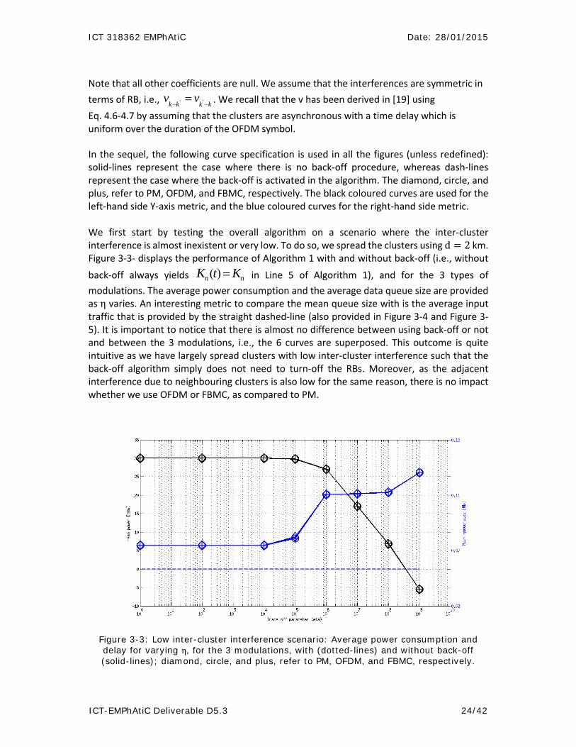
In the sequel, the following curve specification is used in all the figures (unless redefined): solid‐lines represent the case where there is no back‐off procedure, whereas dash‐lines represent the case where the back‐off is activated in the algorithm. The diamond, circle, and plus, refer to PM, OFDM, and FBMC, respectively. The black coloured curves are used for the left‐hand side Y‐axis metric, and the blue coloured curves for the right‐hand side metric. We first start by testing the overall algorithm on a scenario where the inter‐cluster interference is almost inexistent or very low. To do so, we spread the clusters using d 2 km. Figure 3‐3‐ displays the performance of Algorithm 1 with and without back‐off (i.e., without

back‐off always yields nn KtK )( in Line 5 of Algorithm 1), and for the 3 types of

modulations. The average power consumption and the average data queue size are provided as η varies. An interesting metric to compare the mean queue size with is the average input traffic that is provided by the straight dashed‐line (also provided in Figure 3‐4 and Figure 3‐5). It is important to notice that there is almost no difference between using back‐off or not and between the 3 modulations, i.e., the 6 curves are superposed. This outcome is quite intuitive as we have largely spread clusters with low inter‐cluster interference such that the back‐off algorithm simply does not need to turn‐off the RBs. Moreover, as the adjacent interference due to neighbouring clusters is also low for the same reason, there is no impact whether we use OFDM or FBMC, as compared to PM.

Figure 3-3: Low inter-cluster interference scenario: Average power consumption and delay for varying η, for the 3 modulations, with (dotted-lines) and without back-off (solid-lines); diamond, circle, and plus, refer to PM, OFDM, and FBMC, respectively.



Let us now assess the algorithm performance when the clusters are close to each other such that the interference may be high (depending on the transmit power). It is important to note that even links from nearby clusters may succeed to transmit their data, thanks to relative distances that may yield good SINR. Taking for example the links depicted in Figure 3‐2, link 11 may certainly get bad SINR if link 9 transmits, but can succeed if instead of link 9 it is for example link 7 which uses the same RB. But of course, in the long run, the RRM algorithm not using the back‐off algorithm should yield larger delay. Figure 3‐4 a) presents the same comparison as in Figure 3‐3 with now d 100 m to model possible high inter‐cluster interference. In particular, it is important to observe the average queue size (delay). We first note, that for any η, the delay is always lower when using the back‐off algorithm compared to not using it. This is of course a desired behaviour. This is especially true for η small. This is because as η becomes small, the average transmit power increases (close to P ), such that links from nearby clusters are more likely to always interfere each other. Thus, the use of the RBs back‐off becomes very relevant. Now, when η increases, and the transmission power diminishes, the maximum interfering region of each cluster diminishes, such that two simultaneously transmitting links get better and better SINR (of course the transmit power cannot be arbitrarily small since the SINR even with vanishing interference is limited by the receiver noise level, N0). Thus, back‐off becomes less necessary such that the performances between PM, FBMC and OFDM become approximately the same.

It is important to note that, as for the basic backpressure algorithm, increasing infinitely the parameter, does not continuously decrease the transmit power. This is because, as the

transmit power becomes close to the optimal minimum (cannot go lower with queue instability), the data queues will start increasing steadily, and thanks to the counter effect of

the queues in the optimization problem (i.e.,

nMm

mmm tpttq )()()( ), any high η will always

be compensated at some time by the increasing queue. However, this may yield undesirable delays (i.e. time for the queues to be large enough to compensate for η).

a) Average power consumption and delay for varying η.



b) Average delay and theoretical throughput for the associated power consumption

Figure 3-4: High inter-cluster interference scenario: for the 3 modulations, with (doted-lines) and without back-off (solid-lines); diamond, circle, and plus, refer to PM, OFDM,

and FBMC, respectively.

Another point to notice is that one would always expect that the delay performance for the PM is always lower than for the FBMC and itself lower than OFDM. However, Figure 3‐4 a) does not always reflect that intuitive relation. Although the differences quite vanish using the back‐off algorithm, they are well pronounced when not using the back‐off. In order to further investigate this effect, we plot Figure 3‐4 b) for the same performance as in Figure 3‐4 a) but using different axis. This figure better reflects the performance (delay and theoretical throughput) in terms of the effective depleted power instead of η (since for a given different settings can yield different average transmit power). In the second figure, the difference of performance between the 3 modulations is not significant in terms of the average queue. However, when observing the theoretical throughput, )(t , we note that the expected

performance ranking between the 3 modulations is always respected, i.e., PM higher than FBMC and itself better than OFDM.

In Figure 3‐4 we assessed the algorithm performance for some high rate traffic. We provide the same results in Figure 3‐5 using lower traffic input (simply dividing by 1000 the input bits). It is very clear that there is no much difference between using or not the back‐off (or quite small). As explained earlier, even links from nearby clusters can well communicate simultaneously depending on the geographical location (thus their channel quality), as far as the SINR is good enough. Thus, since the traffic is much smaller than in Figure 3‐4, the few times when link 11 and link 7 are luckily scheduled at the same time (i.e., no much self interference) is enough to deplete the small data queues. Thus, back‐off is not very crucial, as opposed to the high traffic scenario.



a) Average power consumption and delay for varying η

b) Average delay and theoretical throughput for the associated power consumption

Figure 3-5: High inter-cluster interference scenario but lower traffic input compared to Figure 3-4 (divided by 1e3): for the 3 modulations, with (dotted-lines) and without back-off (solid-lines); diamond, circle, and plus, refer to PM, OFDM, and FBMC, respectively.

In all the previous performance assessments, we assumed that all signalling broadcasts where always successfully received by all neighbour clusters. However, in practice the broadcast can be lost due to collisions. In order to model this important real constraint, we randomly impose some broadcasts losses at each neighbour cluster. As such we analyse the delay performance as the probability of correctly receiving a broadcast varies. In particular, we do this test for

two parameters, 210 and

510 , i.e. yielding high and low transmission power. We



observe in Figure 3‐6 a), for 210 , that as the probability of correctly receiving the broadcast

diminishes, the delay increases. However, when observing Figure 3‐6 b), for 510 , that the

deterioration becomes less obvious. These are expected results, since as increases, the transmission power diminishes along with the inter‐cluster interferences such that the back‐off algorithm becomes less important. Thus, the frequency update of the signalling message

n also becomes less important.

210

510

Figure 3-6: Delay performance for varying probability of correctly receiving the broadcast, for the 3 modulations; diamond, circle, and plus, refer to PM, OFDM, and

FBMC, respectively.



It is also important to emphasize the nature of the broadcasted information, , which is the data quantity. When transmitting that quantity in a real system, it is most probably required to quantize that information. However, for such type of information quantization loss may not necessarily impact the performance of the algorithm. This of course depends on the overall queues’ size. In other word, having 1 Mb difference for an average traffic of the order of few Mb is more critical than for traffics of the order of tens or hundreds of Mb.

3.4 Performance summary

Here is the performance summary of the proposed new algorithm taking advantage of the SINR information:

As for the classical back‐pressure algorithm, increasing the trade‐off parameter η decreases the energy consumption. This helps neighbour clusters to interfere less among each other such that can have acceptable SINR when communicating at the same time. However, using arbitrarily large η will yield unreasonable delays.

The performance deterioration with lower successful broadcast is more visible when clusters interfere more each other, i.e., nearby clusters use high transmit powers, such that information update about other clusters state becomes more important.

The difference in performance between the three types of modulations becomes small when using the back‐off algorithm since the direct channel interference is better controlled. This is thanks to the orthogonality in transmission obtained using the back‐off algorithm when inter‐cluster interference is too high.

Although, the difference in delay performance is not significant, the better performances of PM over FBMC, itself over OFDM is clear in terms of throughput. This is especially true when the power transmission is high. In practice, some system can only work in an ON/OFF transmission fashion or with restricted set of power transmission. In such a case the use of Back‐off is very useful.

To summarize, the back‐pressure algorithm provides a trade‐off between long‐term energy reduction and system latency, thanks to the tunable η parameter. As a simple example, right after a disaster, much voice traffic with stringent quality may be necessary. This would require low η parameter for the algorithm, accepting the fact the energy depletion is not the most important. Then, few days later,, high quality photos or video of the area may be needed to be transmitted for a long period. In such a case, one would use higher η parameter, accepting the fact that the communication latency can be higher but with more efficient usage of the energy storage. In addition to the salient feature of the back‐pressure algorithm, the back‐off feature is important in a distributed clusterised network where inter‐cluster interference may be high. The idea for the back‐off on top of the back‐pressure algorithm is based on the important fact that when the cross‐talk interference is higher than some threshold, the best communication is an orthogonal‐type communication like FDMA [14]. Of course, to back‐off or not depends on many criteria for each independent and selfish (most probably) cluster The back‐off is done without agreement between clusters but independently based on broadcast signaling sent by the different CHs. That signaling is limited in capacity and the overall algorithm is quite robust to some loss.



4. Scheduling algorithms for FBMC systems

4.1 Introduction It is well‐known that the merits of OFDM come with the cost of transmitting redundancy in the form of a cyclic prefix (CP) and shaping the subcarrier signals with the rectangular window. A viable alternative is the FBMC modulation scheme [20], which does not transmit the CP and shapes subcarriers with well‐frequency‐localized waveforms. The price that is paid to refrain from transmitting a CP is a weak orthogonality that it is only satisfied in the real domain. Thus, multipath fading ruins the orthogonality of FBMC. This is the main obstacle to extend FBMC to multiple‐input‐multiple‐output (MIMO) architectures [21], which is crucial to enhance the performance. Knowing that the solutions devised for OFDM cannot be applied to FBMC in general, several techniques have been proposed to combine MIMO and FBMC [22]. One of the few works that addresses the resource allocation problem in the FBMC context is presented in [23], where the rate in the multiple access channel is maximized given power and users’ rate constraints. In [24] the authors seek for maximizing the downlink capacity of cognitive radio systems. By contrast, the work presented in this section aims at minimizing the transmit power in the downlink subject to users’ rate constraints. The propagation conditions considered in previous works are such that the interference can be neglected [24], or cancelled out by applying the same signal processing techniques as in OFDM [23]. This is not the case in this section, where the channel is more frequency selective revealing that the signal received by each user is affected by inter‐user interference if the user allocation is different in adjacent subcarriers, i.e. when the active users is not the same. To overcome this issue we propose to assign subcarriers to users in a block‐wise fashion. Then, we demonstrate that FBMC systems can benefit from the algorithms proposed in [25] to solve the margin adaptive problem. It is important to remark that this section focuses on multi‐user multiple‐input‐single‐output (MU‐MISO) communication systems, because in this configuration FBMC exhibits robustness against the frequency selectivity, while it achieves the same spatial channels gains as OFDM [26]. The main contribution of this section consists in modifying the scheduling algorithm presented in [25] according to the FBMC transmission scheme, by proposing a specific subcarrier grouping and taking into account the existence of inter‐user, inter‐symbol and inter‐carrier interference.

4.2 System model

Consider the downlink of a MU‐MISO communication system where the terminals and the base station (BS) are equipped with a single and antennas, respectively. The BS uses the spatial dimension to simultaneously serve up to users in the same frequency resources. When the FBMC transceiver is considered, the signal received by the lth user after demodulating the qth subcarrier is [26]:



(4‐1)

. . . (4‐2)

1 even

odd, (4‐3)

for 0 1 and 1 . Let be the noise that contaminates the reception

of the lth user on the qth subcarrier, which follows this distribution ∼ 0, . The

channel frequency response is assumed flat at the subcarrier level. In this sense, the term ∈ denotes the MISO channel frequency response seen by the lth user on the mth

subcarrier. The sequence is frequency multiplexed on the mth subcarrier and it contains real‐valued PAM symbols that are intended for the uth user. Note that is

linearly precoded with ∈ . The coefficients denote the intrinsic

interference and they are defined as

∗ ∗↓

(4‐4)

, (4‐5)

where ∗ denotes convolution. Note that is the subband pulse that is obtained by frequency shifting the low‐pass prototype pulse the length of which is . In this section we opt for the design described in [27] with an overlapping factor equal to four. The operation

. ↓ performs a decimation by a factor of . In the q even case takes the values

gathered in Table 1. The same magnitudes hold when q is odd but the sign may vary. To get rid of the interferences is post‐processed as follows:

∗

, ,, ,

∗

∗ .

(4‐6)

Note that the equalizer is constrained to be real‐valued [26].

k=‐3 k=‐2 k=‐1 k=0 k=1 k=2 k=3

‐j0.0429 ‐0.1250 j0.2058 0.2393 ‐j0.2058 ‐0.1250 j0.0429

‐0.0668 0 0.5644 1 0.5644 0 ‐0.0668

j0.0429 ‐0.1250 ‐j0.2058 0.2393 j0.2058 ‐0.1250 ‐j0.0429 Table 1: Intrinsic interferences under ideal propagation conditions

4.3 SDMA with block diagonalization

One solution to achieve spatial division multiple access (SDMA) consists in following the block diagonalization (BD) approach [28]. Although the BD technique succeeds in achieving interference‐free data multiplexing, it imposes in MU‐MISO communication systems. It can be checked that the subband processing proposed in [26] guarantees that (4‐6)



is free of inter‐symbol interference (ISI), inter‐carrier interference (ICI) and inter‐user interference (IUI), as long as the users served on a given subcarrier are the same on adjacent subcarriers. Then, the maximum achievable rate becomes

1

2log 1 (4‐7)

/0.5 , (4‐8)

where ∈ spans the null space of

⋯ ⋯ . (4‐9)

Note that the power allocated to is given by . The factor in (4‐7) has to do with the

fact that the variables in (4‐6) are real‐valued. To get (4‐7) we assume a continuous transmission, so that the tailsof the pulse have no impact on the rate. This does not hold true in burst‐like transmission, but we leave this case for future work. In the OFDM counterpart

the rate is given by (4‐7) but the factor is dropped because the information is conveyed in

both the in‐phase and quadrature components, i.e. the rate is formulated as

log 1 2 / . (4‐10)

The SINR is not modified but there are two aspects that have to be taken into account. The first one is that the power of the desired signal is multiplied by two since the symbols

transmitted in OFDM are drawn from the QAM scheme and the real‐valued symbols

are obtained from either the real or the imaginary parts of the QAM constellation points. The second relevant aspect has to do with the fact that the power of the noise is not halved because detection is performed in the complex domain. Let us stress that when the power coefficients, the bandwidth and the sampling frequency are kept unchanged in both modulations, then the rate expressed in bps is the same in FBMC and OFDM without CP. To ease the comparison between FBMC and OFDM we consider the rate that corresponds to one OFDM symbol period. Thus, the rate that will be used from this point on unless otherwise stated is expressed in this form

log 1 , (4‐11)

which is valid for both modulations. Bearing in mind that (4‐11) is achieved in FBMC systems by transmitting two multicarrier symbols, it follows that the total transmitted power in one

OFDM symbol period is ∑ ∑ 2 . By contrast, taking into account that the symbols in

OFDM are obtained from a complex‐valued constellation diagram, the transmitted power in

OFDM is equal to ∑ ∑ 1 2 , where denotes the CP length. For the sake

of clarity the CP will be only considered when the transmitted power is computed and will be neglected when the rate is evaluated.

4.4 Margin adaptive scheduling algorithm

It is worth emphasizing that when the BS selects out of users over each subcarrier. However, the user assignment has to remain constant over all subbands so that the BD approach is able to remove the ICI in FBMC. This can be easily proved as follows. Consider a toy example where 2 users are allocated in each subcarrier. Imagine that subcarriers 1, 1 are assigned to the users and , while the users and are

allocated in the qth subcarrier. If and are designed according to [26], we get



∗

∗ ,

(4‐12)

for 1,2. Note that in (4‐12) there is no contribution from user for . On the negative

side, we cannot neglect the ICI because the precoding vectors do not satisfy .

Hence, (4‐12) shows the situations that should be avoided to get rid of the interference. To guarantee that all users achieve a certain rate in the absence of interference, we propose to assign subcarriers to users in a block‐wise fashion. In other words, the band is partitioned into

subsets, where the subset encompasses these subcarrier indexes 1 , . . . , 1

assuming that is an integer number. Taking into account that the roll‐off factor of the

prototype pulse is close to one, the first carrier of each set is left empty to isolate the blocks.

Based on that we define 1 for all .

In the light of the above discussion, the optimization problem is posed as follows:

argmin,

∈

. . l

∈

og 1 , 1

, ∈ 0,1 , 1 .

(4‐13)

By solving (4‐13) we find the optimal user selection and power allocation, so that the users’ rate constraints are guaranteed with the minimum transmit power. Note that the channel

gains defined in (4‐8) depend on the channel interference matrix, which in turns depend

on the subcarrier assignment. With the aim of substantially reducing the complexity, we assume that constant power is used on each block. Then the number of variables to optimize is significantly reduced and the problem can be simplified as

argmin,

| |

. . l

∈

og 1 , 1

, ∈ 0,1 , 1 ,

(4‐14)

where | | 1 and denotes the power that user assigns to all subcarriers that belong

to . By mapping the sum of rates into a single metric we get more tractable expressions. In this regard, we consider this inequality



l

∈

og 1 | |log 1 , (4‐15)

where

∈

/| |

(4‐16)

is the geometric mean [29]. By substituting the sum of rates by the right hand side of (4‐15), we can reformulate (4‐14) as

argmin,

| |

. . | |log 1 , 1

, ∈ 0,1 , 1 .

(4‐17)

Now the blocks play the same role as subcarriers and, thus, we can take advantage of existing low‐complexity algorithms, see e.g. [25]. The solution of (4‐17) guarantees that the original rate constraints in (4‐13) are satisfied because of the inequality established in (4‐15).

4.5 Successive channel allocation This section focuses on solving (4‐17) by using the linear programming based successive channel allocation (LPSCA) algorithm described in [25]. Among the possible choices we have favored the LPSCA because it exhibits an excellent tradeoff between complexity and performance. The LPSCA was initially though for OFDM systems, which highlights that it may not be easily tailored to the FBMC scheme. To cast some light into the applicability of the LPSCA to FBMC systems this section briefly describes the algorithm to be employed and the necessary modifications due to the characteristics of the transmitted signal. The main asset of the LPSCA stems from the reduction of the complexity that is achieved by grouping users into disjoint sets, so that 1, . . . , ⋃. . . ⋃ . The partitioning is

made according to the average channel quality assessment [25]. Then, (4‐17) is also partitioned into independent problems that are sequentially optimized. First we allocate the most distant users to the BS, which means that we start with subset and we terminate with the subset . When subset is addressed, the users that belong to , for have

already been allocated. To guarantee that the rate constraints are not violated, the subband processing is designed to prevent signals that are intended to users in from leaking through users that belong to , for . In the rest of the section we focus on the subset without

loss of generality. In this sense, the signal received by the user ∈ is

∗ , (4‐18)

where



∈

∗

, ,

∗

.

(4‐19)

The already allocated users in the mth subcarrier when the subset is addressed, are

included in this set and, thus, ⊆ ⋃ . Now the transmit processing is designed

to project the channel onto the null space of

⋯ . (4‐20)

Let denote the jth element of subset . Bearing (4‐20) in mind, and are

designed as [26] proposes in order to remove the interference, yielding

(4‐21)

, (4‐22)

where ∈ spans the null space of (4‐20). Then, ∗

0, for , , 0 . Since the users in cannot claim protection

against the users in , for , the first term of (4‐19) is not removed and the variance of

the noise plus the interference becomes

∗

∈

0.5 .

(4‐23)

Considering the values of Table 1 along with the fact that the same users are allocated in adjacent subcarriers, i.e. = = , (4‐23) can be expressed as

0.5

∈

0.646 0.1769

0.1769 .

(4‐24)

If the channel frequency selectivity is not severe we can assume that

, . (4‐25)

Then, it follows that (4‐24) can be approximated by

0.5

∈

. (4‐26)

When the subset is addressed 0.5 . In the general form the rate is given by

log 1 (4‐27)

/ . (4‐28)



Once the interference is updated, the problem associated to the subset is

: argmin,

| |

∈

. . | |log 1 , ∈

∈

1, ∈ 0,1 , 1 ,

(4‐29)

where

∈

/| |

. (4‐30)

Similarly to problem (4‐17), the users’ rate constraints and the objective function have been defined taking into account that the power within each block is constant. The approximation made in (4‐25) results in (4‐28), which exactly coincides with the SINR that is obtained in OFDM when the sequential channel assignment approach is implemented [25]. Hence, the solution of (4‐29) can be indistinctly used in OFDM and FBMC systems. As it has been mentioned we propose to solve (4‐29) by executing the LPSCA algorithm that is described in [25].

4.6 Numerical results

This section is devoted to evaluating the user selection and the power allocation algorithm proposed in Section 4.5. Regarding the system parameters, the bandwidth is 10 MHz, the number of subcarriers is 1024 and the sampling frequency is set to 15.36 MHz so that the subcarrier spacing is Δ 15 kHz. . Similar settings have been selecting in Section 3 (e.g.

Δ 15 kHz and B=1.4MHz). The number of users that are connected to the BS is equal to

10 and they are uniformly distributed in a cell of radius 500 m. Since the number of transmit antennas is set to 2, only two users can be associated with each subcarrier. The thermal noise density is ‐174 dBm/Hz and the channel is modeled as a Rayleigh fading process with a power delay profile that follows the extended pedestrian A (EPA) channel model [30]. The path loss exponent is 4. It should be mentioned that the frequency selectivity of the EPA channel is such that the system model described in Section 4.2 is valid. In other words, the channel frequency response can be assumed flat at the subcarrier level. Concerning the air‐interface, we consider FBMC and OFDM with a CP that encompasses /14 samples. To comply with the recommendations proposed by the Technical

Specification Group for Radio Access Network of the 3GPP, only 600 out 1024 subcarriers are used to transmit data. Furthermore, subcarriers are gathered in RBs of 12 and, thus, there are

50 RBs. In notation terms, let denote the set whose elements are the indexes of those subcarriers that are active and indicates the ith active subcarrier. Borrowing the

notation from Section 4.5, the elements of subset when OFDM is implemented are given

by 1 12 1 . . . 12 , for 1, . . . ,50. To prevent ICI from degrading the FBMC

system performance, the blocks are separated by one subcarrier that is intentionally left empty. Then in FBMC the number of subcarriers that are able to convey data is extended from

600 to 650 and the subsets are generated as 2 13 1 . . . 13 , for

1, . . . ,50. Although inserting one guard band between blocks increases the out of band



radiation, the transmitted signal in FBMC still fits into the spectrum mask of the Universal Mobile Telecommunication System (UMTS) [31]. Actually, it is shown that the occupied subcarriers can be increased in 10 % without violating the spectrum mask. The Figure 4‐1 depicts the power that is required to schedule 10 users in 50 blocks of 12 subcarriers each. As it has been pointed out in Section 4.4, one subcarrier is left empty between blocks when the FBMC modulation is employed. It should be emphasizing that this does not mean that interference is removed, but the RBs do not interfere each other. The

metric that is evaluated is ∑ ∑ 12 1 / 2 , where the power coefficients

have been obtained after solving (4‐29). The rate constraints have been set equal for all users as follows: 600/ , where is the target spectral efficiency. It is important to recall that 0 in FBMC systems, and because of that the transmitted power is reduced when compared to OFDM, as Figure 4‐1 highlights. In order to verify that both modulations are able to achieve similar rates we have depicted in

Figure 4‐2 the overall rate, which is defined as ∑ ∑ ∈ . To this end we have used the

exact rate definition given by (4‐27). Nevertheless, the power of the residual interference plus noise in OFDM and FBMC systems is characterized by (4‐26) and (4‐24), respectively. In the light of the results of Figure 4‐2 we can conclude that the assumption made in (4‐25) does not have any negative impact as the overall rates achieved in both modulation schemes practically coincide. Another important aspect that is worth highlighting is that the relative difference between the exact sum‐rate and the lower bound based on the geometric mean, which is formulated in (4‐15), does not exceed 0.25% after solving (4‐29). This holds true for OFDM and FBMC, which supports the simplifications proposed in this section. For the sake of the clarity in the presentation of the results the lower bound has not been included in Figure 4‐2.

Figure 4-1: Power vs. spectral efficiency in OFDM and FBMC.



Figure 4-2: Overall rate vs. spectral efficiency in OFDM and FBMC.

4.7 Conclusions This section shows that the joint optimization of transmit and receive beamforming, the channel assignment and the power allocation is very challenging in the FBMC context. The main reason stems from the fact that the received signals are subject to inter‐user, inter‐carrier and inter‐symbol interference. By grouping subcarriers and keeping the same user selection and power allocation in each group we can exploit spatial diversity to allocate several users in the same frequency resources. It has been demonstrated that the margin adaptive problem in OFDM and FBMC systems can be sub‐optimally solved resorting to the LPSCA method. Since no energy is wasted in the FBMC modulation scheme, this modulation is able to transmit the same amount of information as OFDM but using less power.



5. Conclusions

In this report, Radio Resource Management for PMR communications based on FBMC has been investigated. The different techniques presented are further improvements of D5.2, that take into account cross‐layer interactions between RRM and both physical and application layers.

The problems considered in this deliverable are all very relevant to PMR communications: voice communications, buffer queue stabilization and energy consumption minimization, power consumption minimization in multiple antennas context.

First, the critical problem of voice communications for PMR communications in cell‐based scenario has been studied in Section 2. The E‐model has been chosen to model the MOS of voice communications. It provides an efficient way of involving application layer performance metrics in RRM algorithms. The proposed algorithm adapts the encoding rate of voice service depending on the end user’s QoE. It provides a high capacity gain compared to non‐adaptive algorithms.

In Section 3, the DUST algorithm, initially introduced in D5.2, has been further improved. It implies cross‐layer optimization between RRM and the physical layer, with the objective to achieve a stable buffer queue for all users and to minimize energy consumption. The clustered scenario implies inter‐cluster interference due to lack of synchronization. In this context, FBMC is known to achieve better performances than CP‐OFDM. The achieved performances in terms of delay depend on the multi‐carrier modulation and on the back‐off algorithm. As the back‐off algorithm leads to an orthogonal transmission, the performances are almost the same with all multi‐carrier modulations (FBMC, CP‐OFDM and Perfect Modulation). If the back‐off algorithm is not used, the delay differences between the modulations increase.

Finally, Section 4 has introduced a scheduling algorithm for solving the margin adaptive problem MU SIMO with CP‐OFDM and FBMC. In SIMO, inter‐user, inter‐carrier and inter‐symbol interferences must be dealt with. In order to allocate several users in the same frequencies and thus exploit spatial diversity, it is necessary to group subcarriers and allocating the same users with the same power allocation within each subcarriers group. Then the margin adaptive problem can be solved sub‐optimally using the LPSCA (linear programming based successive channel allocation) method. FBMC leads to a power consumption decrease compared to OFDM.



6. References

[1] Deliverable D5.2, “Novel algorithms description and performance evaluation for RRM

in cell‐based and ad‐hoc PMR networks”, FP7 EMPHATIC project.

[2] Y. Wardi, B. Melamed, “Variational bounds and sensitivity analysis of traffic processes

in continuous flow models”, Springer’s Discrete Event Dynamic Systems, vol. 11, no. 3,

pp. 249–282, 2001.

[3] Y. Wardi, B. Melamed, “Loss volume in continuous flow models: Fast simulation and

sensitivity analysis via IPA”, Proceedings of 8th IEEE Mediterranean Conference on

Control and Automation (MED 2000), July 2000.

[4] B. Liu,Y. Guo, J. Kurose.,D. Towsley. W.B. Gong, “Fluid simulation of large scale

networks: Issues and tradeoffs”, Proceedings of International Conference on Parallel

and Distributed Processing Techniques and Applications, June 1999.

[5] K. Kumaran, D. Mitra, “Performance and fluid simulations of a novel shared buffer

management systems”, ACM Transactions on Modeling and Computer Simulation

(TOMACS), vol. 11, no. 1, pp. 43–75, 2001.

[6] A. Yan, W.B. Gong, “Fluid simulation for high speed networks with flow‐based

routing”, IEEE Transactions on Information Theory, vol. 45, no. 5, pp. 1588–1599, 1999.

[7] ITU‐T: Methods for Subjective Determination of Transmission Quality. Rec. P.800,

1996.

[8] ITU‐T: Single‐ended method for objective speech quality assessment in narrow‐band

telephony applications. Rec. P.563, 2005.

[9] ITU‐T: The E‐Model: A Computational Model for Use in Transmission Planning. Rec.

G.107, 2012.

[10] S. Jadhav, H. Zhang, Z. Huang, “MOS‐based Handover Protocol for Next Generation

Wireless Networks”, IEEE 26th International Conference on Advanced Information

Networking and Applications, pp. 479–486, 2012.

[11] J. Fitzpatrick, "An E‐Model based adaptation algorithm for AMR voice calls," Wireless

Days (WD), IFIP , vol., no., pp.1‐6, 10‐12 Oct. 2011.

[12] F. Mertz and P. Vary, “Efficient voice communication in wireless packet networks,” in

Proceedings of Sprachkommunikation, ITG‐Fachtagung, 2008, pp. 92–99. [Online].

Available: http://www.vdeverlag.de/proceedings‐de/453120011.html

[13] L. Georgiadis, M. J. Neely, L. Tassiulas, ”Resource allocation and cross‐layer control in

wireless networks”, Foundations and Trends in Networking, vol.1, no. 1, 1144, 2006.

[14] S. Hayashi, ZQ Luo, “Spectrum Management for Interference‐Limited Multiuser

Communication Systems”, IEEE Trans. Inform. Theory, vol 55, no. 3, pp. 1153 – 1175,

March 2009.

[15] M. J. Neely, Dynamic Power Allocation and Routing for Satellite and Wireless Networks

with Time Varying Channels. PhD thesis, LIDS, MIT, Cambridge, MA, 2003.

[16] X. Tan, Z. Xiong, and Y. He, “Signal Attenuation‐aware Clustering in Wireless Mobile

Ad Hoc Networks”, Journal of Networks, vol. 8, no. 4, pp.796‐803, Apr. 2013.



[17] R. Ghosh and S.Basagni, “Mitigating the impact of node mobility on ad hoc clustering,”

Wireless Communications and Mobile Computing, vol. 8, no. 3, pp 295‐308, Mar. 2008.

[18] Deliverable D9.1, “Definition and specification of hardware demonstrator and

software simulator”, FP7 EMPHATICc project.

[19] Deliverable D5.1, “Study of the advantages of FBMC in RRM for PMR”, FP7 EMPHATIC

project.

[20] P. Siohan, C. Siclet, N. Lacaille, “Analysis and design of OFDM/OQAM systems based

on filterbank theory”, IEEE Transactions on Signal Processing, vol. 50, no. 5, pp. 1170

–1183, May 2002.

[21] B. Farhang‐Boroujeny, “OFDM Versus Filter Bank Multicarrier,” Signal Processing

Magazine, IEEE, vol. 28, no. 3, pp. 92 –112, May 2011.

[22] M. Caus, MIMO Designs for filter bank multicarrier and multiantenna systems based

on OQAM, Ph.D. dissertation, Universitat Politecnica de Catalunya (UPC), 2013.

[Online]. Available: http://theses.eurasip.org

[23] M. Payaro, A. Pascual‐Iserte, A. Garcia‐Armada, M. Sanchez‐Fernandez, “Resource

Allocation in Multi‐Antenna MAC Networks: FBMC vs OFDM,” in Vehicular Technology

Conference (VTC Spring), 2011 IEEE 73rd, May 2011.

[24] M. Shaat, F. Bader, “Computationally Efficient Power Allocation Algorithm in

Multicarrier‐Based Cognitive Radio Networks: OFDM and FBMC Systems,” EURASIP

JASP, vol. 2010.

[25] M. Moretti and A. I. Perez‐Neira., “Efficient Margin Adaptive Scheduling for MIMO‐

OFDMA Systems,” Wireless Communications, IEEE Transactions on, vol. 12, no. 1, pp.

278–287, 2013.

[26] M. Caus, A. I. Perez‐Neira, M. Moretti, “SDMA for FBMC with block diagonalization,”

in Signal Processing Advances in Wireless Communications (SPAWC), IEEE 14th

International Workshop on, 2013.

[27] M. Bellanger, “Specification and design of a prototype filter for filter bank based

multicarrier transmission.” ICASSP, 2001, pp. 2417–2420.

[28] Q. H. Spencer, A. L. Swindlehurst, M. Haardt, “Zero‐forcing methods for downlink

spatial multiplexing in multiuser MIMO channels,” Signal Processing, IEEE

Transactions on, vol. 52, no. 2, Feb. 2004.

[29] J. Huang, V. Subramanian, R. Agrawal, and R. Berry, “Downlink scheduling and

resource allocation for OFDM systems,” Wireless Communications, IEEE Transactions

on, vol. 8, no. 1, pp. 288–296, 2009.

[30] 3GPP TS 36.101 V11.8.0, “Evolved Universal Terrestrial Radio Access (E‐UTRA); User

Equipment (UE) radio transmission and reception (Release 11),” 2014.

[31] L. G. Baltar, D. S. Waldhauser, J. A. Nossek, “Out‐of‐band radiation in multicarrier

systems: a comparison,” in Multi‐Carrier Spread Spectrum 2007, ser. Lecture Notes

Electrical Engineering. Springer Netherlands, 2007, vol. 1, pp. 107–116.

[32] X. Tan, Z. Xiong, and Y. He, “Signal Attenuation‐aware Clustering in Wireless Mobile

Ad Hoc Networks,” Journal of Networks, vol. 8, no. 4, pp. 796‐803, 2013.



Glossary and Definitions

Acronym Meaning

3GPP 3rd Generation Partnership Project AMR Adaptive Multi-Rate BS Base StationCFM Continuous Flow Modelling CH Cluster Head CP Cyclic Prefix DMO Direct Mode Operation DUST Distributed bUffer Stabilization RRM algorithm FBMC Filter Bank Multicarrier HH Hand HeldICI Inter-Channel Interference LPSCA Linear Programming based Successive Channel

Allocation MAC Medium access control MCS Modulation and coding scheme MISO Multiple Input Single Output MOS Mean Opinion Score MS Mobile StationMU Multi-User OFDM Orthogonal Frequency Division Multiplexing OFDMA Orthogonal Frequency Division Multiple Access OQAM Offset Quadrature Amplitude Modulation PESQ Perceptual Evaluation of Speech Quality PSQM Perceptual Speech Quality Measure PHY Physical layer PMR Professional Mobile RadioPM Perfect Modulation QoE Quality of Experience RRM Radio Resource Management RS Relay StationRB Resource Block SC-FDMA Single Carrier – Frequency Division Multiple Access SDMA Space Division Multiple Access SIMO Single Input Multiple Output TDMA Time division multiple access

Documents

Enhanced Multicarrier Techniques for Professional Ad … fileTable of Contents 1 ... 2.3.2 Calculation of the timeout rate and delay in discrete time intervals ..... 9 2.4