Active Segmentation of 3D Axonal Images∗

Gautam S. Muralidhar1, Ajay Gopinath2, Alan C. Bovik2, and Adela Ben-Yakar3

Abstract— We present an active contour framework for seg-menting neuronal axons on 3D confocal microscopy data. Ourwork is motivated by the need to conduct high throughput ex-periments involving microfluidic devices and femtosecond lasersto study the genetic mechanisms behind nerve regenerationand repair. While most of the applications for active contourshave focused on segmenting closed regions in 2D medical andnatural images, there haven’t been many applications that havefocused on segmenting open-ended curvilinear structures in 2Dor higher dimensions. The active contour framework we presenthere ties together a well known 2D active contour model [5]along with the physics of projection imaging geometry to yield asegmented axon in 3D. Qualitative results illustrate the promiseof our approach for segmenting neruonal axons on 3D confocalmicroscopy data.

I. INTRODUCTIONUnderstanding the genetic mechanism behind how neu-

rons in the peripheral nervous system repair themselvesafter injury and how they maintain their axonal structureand function over time holds the key to developing bettertreatments for neurodegenerative diseases and nerve injuries.This goal has led to recent advances in developing state-of-the art infrastructure using microfluidic devices and fem-tosecond lasers [1], [2] for performing axotomy on modelorganisms such as the nematode C. elegans. Microfluidicdevices enable easy and efficient handling of C. elegans foraxotomy and imaging without the need for additional im-mobilizing chemicals, while femtosecond lasers have shownto be valuable as a precise cutting tool for severing axonsin C. elegans without heating or damaging the surroundingcells. These devices combined with confocal microscopyimaging allow for a study of axonal repair and the associatedgenetic mechanisms. However, to be able to draw meaning-ful statistical conclusions, it is necessary to perform high-throughput experiments involving many C. elegans worms.High-throughput experiments necessitate automated analysisof the 3D confocal microscopy imaging data after axotomy inorder to quantify changes such as re-growth and reconnectionthat take place along the severed axon. This has resulted inthe development of image analysis techniques for quantifyingneuronal morphology, e.g., [3] and [4].

In this paper, we present an active contour frameworkfor segmenting neuronal axons, which manifest as open-

*This work was supported by the National Institute of Health under grantsRO1 NS060129, R21 NS058646, and R21 NS067340.

1G. S. Muralidhar is with Biomedical Engineering, The University ofTexas at Austin, TX, 78712, USA gautam.sm@utexas.edu

2A. Gopinath and A. C. Bovik are with Electrical and ComputerEngineering, The University of Texas at Austin, TX, 78712, USAajay.gopinath@gmail.com, bovik@ece.utexas.edu

3A. Ben-Yakar is with Mechanical Engineering, The University of Texasat Austin, TX, 78712, USA ben-yakar@mail.utexas.edu

Compute2DForwardProjec3onsofthe3DData

SegmenttheAxonUsinga2DAc3veContourDeployedon

EachProjec3on

ReconstructtheSegmentedAxonin3DbyBack‐Projec3ng

the2DAc3veContourCoordinates

Fig. 1. Proposed framework.

ended curvilinear structures on 3D confocal microscopydata. Active contour models, also known as snakes [6],[7], [8], are commonly employed to represent and trackobjects of interest in natural and medical images. While thetraditional application of active contour models has been therepresentation of closed regions in images, they have beenapplied in a few applications involving segmentation of open-ended curvilinear structures [9], [10], particularly in 3D.Finding and modeling open-ended structures such as axonsinvolves unique challenges such as not knowing the lengthof the axon a priori. We address these questions by joininga well known 2D active contour model [5] with projectionimaging geometry to yield a 3D segmentation of the axon.Preliminary qualitative results illustrate the promise of ourapproach for segmenting neuronal axons on 3D confocalmicroscopy data.

II. PROPOSED FRAMEWORK

The proposed framework is illustrated in Fig. 1. We nextdescribe these steps in detail.

A. Forward Projection

Let f ∈ RN represent the vectorized 3D confocal mi-croscopy data, where N is the total number of voxels. Then,for noise-free data, the forward model can be written as:

g = Hf, (1)

where g is a vector that represents the projection images,and H is the projection matrix, also known as the forwardoperator. The projection matrix H essentially models theimaging process. For example, the coefficients of H couldmodel the attenuation and linear blur mechanisms inherentin the imaging. The coefficients of H serve as weights that

describe the contribution of each voxel in the data f to aparticular projection gi. We assumed the Radon model whiledesigning the projection matrix H , i.e., only those voxels thatlie along a line defined by the coefficients of H contributeto the projection data.

B. 2D Active Contour Model

We next deployed an open-ended parametric 2D activecontour on each projection image generated by the forwardprojection process. A parametric active contour is definedas the parametric curve v(s) = [x(s), y(s)]T , which evolvesthrough the image to minimize the following energy func-tional [6]:

E(v(s)) =∫ 1

0

[12(α|v′(s)|2 + β|v′′(s)|2) + Eext(v(s))

]ds

(2)where v′(s), and v′′(s) are first and second derivatives ofv(s) that represent continuity and tautness of the curve,respectively. The weighting terms α and β determine howmuch importance is placed on the continuity and the taut-ness of the curve, respectively. The terms v′(s), and v′′(s)contribute to the internal energy of the contour, i.e., theenergy that is inherent in the contour. The term Eext(v(s))determines the external energy typically arising from imagefeatures such as edges and is meant to draw the evolvingcontour towards the boundaries of the object of interest.Typical choices of the external energy include variants ofthe image gradient [7], [6]. At a local minima of theevolving curve, the Euler-Lagrange force balanced equationFint+Fext = 0 is satisfied, where Fint = αv′′−βv′′′′ is theinternal force controlling the curve’s continuity and tautness,while Fext = −∇Eext(v) is the external force arising fromimage features such as edges, respectively.

We use the vector field convolution (VFC) formulationfor the external energy term [5]. In the VFC formulation, astandard feature map derived from the image is convolvedwith a user-defined vector field kernel. A requirement on thevector field kernel is that all the vectors in the field shouldpoint towards the kernel origin. Hence, when the kernelorigin coincides with a feature such as an object boundaryor a curvilinear structure, all the vectors in the vector fieldpoint towards this feature, causing the evolving contour tobe deformed towards the feature. The VFC formulation alsoprovides a large capture range for subtle features of interestand is robust to noise [5].

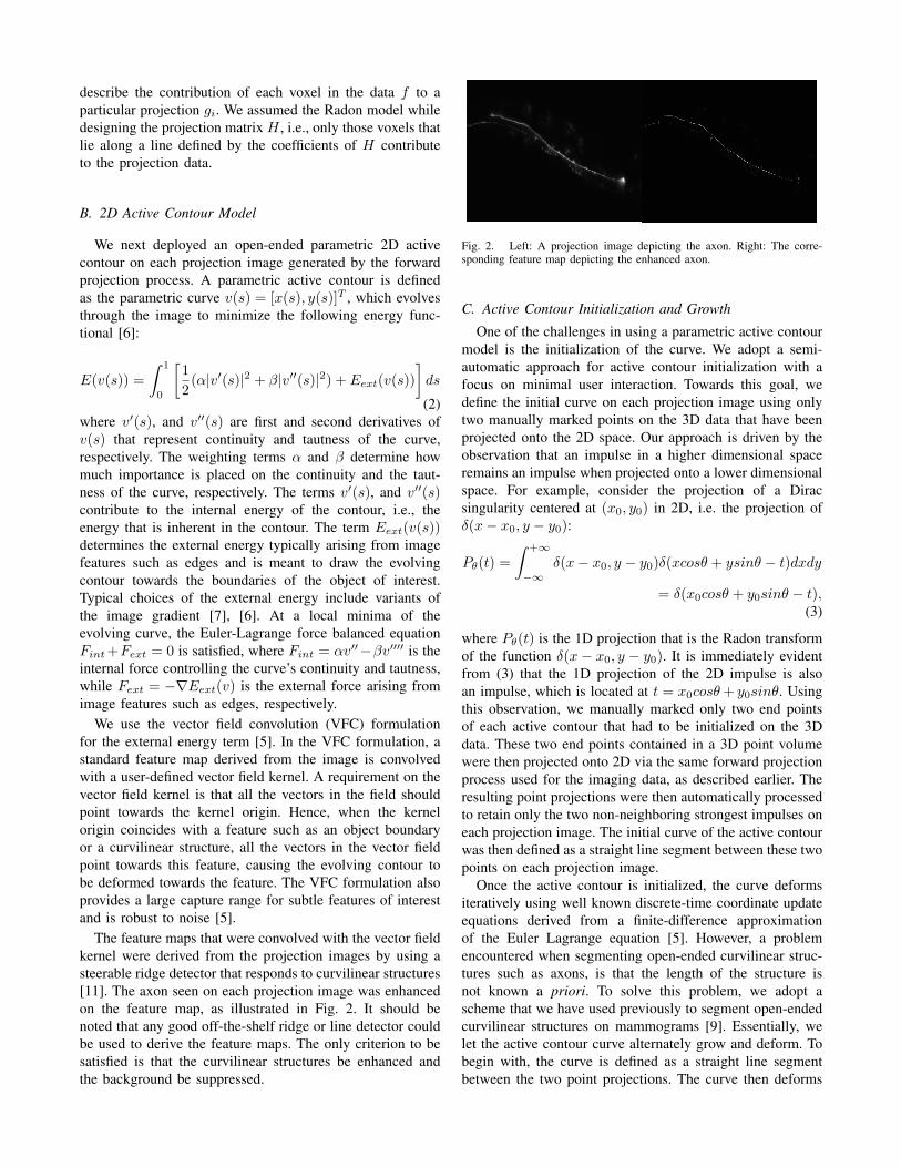
The feature maps that were convolved with the vector fieldkernel were derived from the projection images by using asteerable ridge detector that responds to curvilinear structures[11]. The axon seen on each projection image was enhancedon the feature map, as illustrated in Fig. 2. It should benoted that any good off-the-shelf ridge or line detector couldbe used to derive the feature maps. The only criterion to besatisfied is that the curvilinear structures be enhanced andthe background be suppressed.

Fig. 2. Left: A projection image depicting the axon. Right: The corre-sponding feature map depicting the enhanced axon.

C. Active Contour Initialization and Growth

One of the challenges in using a parametric active contourmodel is the initialization of the curve. We adopt a semi-automatic approach for active contour initialization with afocus on minimal user interaction. Towards this goal, wedefine the initial curve on each projection image using onlytwo manually marked points on the 3D data that have beenprojected onto the 2D space. Our approach is driven by theobservation that an impulse in a higher dimensional spaceremains an impulse when projected onto a lower dimensionalspace. For example, consider the projection of a Diracsingularity centered at (x0, y0) in 2D, i.e. the projection ofδ(x− x0, y − y0):

Pθ(t) =∫ +∞

−∞δ(x− x0, y − y0)δ(xcosθ + ysinθ − t)dxdy

= δ(x0cosθ + y0sinθ − t),(3)

where Pθ(t) is the 1D projection that is the Radon transformof the function δ(x− x0, y − y0). It is immediately evidentfrom (3) that the 1D projection of the 2D impulse is alsoan impulse, which is located at t = x0cosθ+ y0sinθ. Usingthis observation, we manually marked only two end pointsof each active contour that had to be initialized on the 3Ddata. These two end points contained in a 3D point volumewere then projected onto 2D via the same forward projectionprocess used for the imaging data, as described earlier. Theresulting point projections were then automatically processedto retain only the two non-neighboring strongest impulses oneach projection image. The initial curve of the active contourwas then defined as a straight line segment between these twopoints on each projection image.

Once the active contour is initialized, the curve deformsiteratively using well known discrete-time coordinate updateequations derived from a finite-difference approximationof the Euler Lagrange equation [5]. However, a problemencountered when segmenting open-ended curvilinear struc-tures such as axons, is that the length of the structure isnot known a priori. To solve this problem, we adopt ascheme that we have used previously to segment open-endedcurvilinear structures on mammograms [9]. Essentially, welet the active contour curve alternately grow and deform. Tobegin with, the curve is defined as a straight line segmentbetween the two point projections. The curve then deforms

Fig. 3. Growing active contour. top left: initial curve; top right: after 5iterations; bottom left: after 15 iterations, bottom right: after 25 iterations.

under the influence of its internal and external forces fora fixed number of iterations. The deformation is followedby extending the curve along one of it’s end points inthe direction of the tangent computed at that end point byintroducing another short line segment of a predefined length.This new segment then deforms under the influence of itsinternal and external forces for a fixed number of iterations.The process of extension and deformation repeats until astopping criterion is met or a certain number of iterationshave been completed. We do not use a stopping criterionbut rely on a fixed number of iterations, though a stoppingcriterion based on factors such as curvature could easily beincorporated. For instance, in our previous work [9], wehave used a curvature based stopping criterion for open-ended active contours, where the growth of the contour wasterminated at a point where the curvature exceed a 30◦ limit.The predefined length of each extended straight line segmentwas set to an arbitrarily chosen value of 10 pixels and thenumber of iterations of extension and deformation was setto 25. Fig. 3 illustrates four iterations of the growing activecontour along an axon trajectory on one of the projectionimages.

D. 3D Reconstruction of the Axon

Once the 2D active contours have been deployed on eachprojection image and the axon has been segmented in 2D,reconstruction of the 3D axon is performed using the simpleback-projection operator HT , i.e.

fseg = HT gseg, (4)

where gseg is the vectorized projection data containing non-zero values only along the active contour coordinates. Theresult of this operation yields the segmented axon in 3D.

III. EXPERIMENTS AND RESULTSThe data set for this study comprised of a stack of 51

confocal microscopy images depicting the anterior longitu-dinal microtubule (ALM) - a touch receptor neuron in the C.elegans worm. The theoretical resolution of the data was 149

Axotomy region

Original axon trajectory

Re-growth trajectory

Region of study

Fig. 4. Two pairs of initial active contour end-points on a projection image.The blue points represent one pair, while the red points represent the other.Also illustrated are the axotomy region and the two trajectories of the axonpre-and post-axotomy.

nano-meters in the x-y plane, while the resolution along theoptical axis of the microscope (z-direction) was 529 nano-meters. Each image was 2048 × 2048 pixels in dimensionwith 8 bits per pixel. Hence, the dimensions of the 3Dvolume was 2048×2048×51 voxels. For efficient processing,we considered a cropped 3D volume that best depicted theaxon. The dimensions of the cropped volume was 1549 ×901×28 voxels. The forward projections were then computedon the cropped volume. For the forward projection Radonmodel, we considered 91 angular increments from -45 to + 45degrees. Each projection image was further sub-sampled bya factor of two to accelerate processing. The active contoursand the subsequent 3D reconstruction of the segmented axonwere then carried out on the sub-sampled projections. Wemanually initialized two pairs of end points on a 3D slice bestdepicting the region where the axon had been severed. Thesetwo pairs of points were then projected onto the projectionspace using the same forward projection model used for theimaging data. The projected points are illustrated in Fig. 4along with the region where the axon was severed. Alsoillustrated in Fig. 4 are the original and axon re-growth tra-jectories pre- and post-axotomy. The 3D rendering of the seg-mented axon trajectories is illustrated in Fig. 5. We used theopen source software VolRover (http://cvcweb.ices.utexas.edu/cvcwp/?page_id=100) to perform 3Dvolume rendering and visualization. It is evident from Fig. 5that the two active contours were able to capture, segment,and accurately represent the original axon trajectory as wellas the re-growth trajectory after axotomy.

IV. CONCLUSION

We have presented a framework for reconstructing andrepresenting neuronal axons in 3D from confocal microscopyimaging data. The basic framework can be extended torepresent open-ended curvilinear structures on other multi-slice imaging modalities that follow the principles of projec-tion imaging geometry. Future work includes a quantitativevalidation of the framework, and modeling the repair andregeneration of multiple 3D neuronal axons from confocalmicroscopy images acquired after axotomy on a large num-ber of C. elegans worms.

Fig. 5. 3D rendering and visualization of the active contours.

ACKNOWLEDGMENT

The authors would like to thank Frederic Bourgeois foracquiring and supplying the confocal microscopy data.

REFERENCES

[1] S. X., Guo, F. Bourgeois, T. Chokshi, N.J. Durr, M. Hilliard, N.Chronis, and A. Ben-Yakar, Femtosecond laser nanoaxotomy lab-on-a-chip for in-vivo nerve regeneration studies, Nature Methods, vol. 5,pp. 531-533, Jun. 2008.

[2] F. Yanik, H. Cinar, N. Cinar, A. Chisholm, Y. Jin, and A. Ben-Yakar,Neurosurgery: Functional regeneration after laser axotomy, Nature,vol. 432, pp. 822, Dec. 2004.

[3] Y. Zhang, X. Zhou, J. Lu, J. Lichtman, D. Adjeroh, and S. T. C. Wong,3D axon structure extraction and analysis in confocal fluorescencemicroscopy images, Neural Computation, vol. 20, pp. 1899-1927, Aug.2008.

[4] D. E. Donohue and G. A. Ascoli, Automated reconstruction ofneuronal morphology: An overview , Brain Research Reviews, vol.67, pp. 94-102, Jun. 2011.

[5] B. Li and S. T. Acton, Active contour external force using vectorfield convolution for image segmentation, IEEE Transactions on ImageProcessing, vol. 16, pp. 2096-2106, Aug. 2007.

[6] M. Kass, A. Witkin, and D. Terzopoulos, Snakes: active contourmodels, International Journal of Computer Vision, vol. 1, pp. 321-331, Apr. 1988.

[7] X. Chenyang and J. L. Prince, Snakes, shapes, and gradient vectorflow, IEEE Transactions on Image Processing, vol. 7, pp. 359-369,Mar. 1998.

[8] T. F. Chan and L. A. Vese, Active contours without edges, IEEETransactions on Image Processing, vol. 10, pp. 266-277, Feb. 2001.

[9] G. S. Muralidhar, A. C. Bovik, J. D. Giese, et al., Snakules: Amodel-based active contour algorithm for the annotation of spiculeson mammography, IEEE Transactions on Medical Imaging, vol. 29,pp. 1768-1780, Oct. 2010.

[10] M. B. Smith, L. Hongsheng, T. Shen, et al., Segmentation and trackingof cytoskeletal filaments using open active contours, Cytoskeleton, vol.67, pp. 693-705, Nov. 2010.

[11] M. Jacob and M. Unser, Design of steerable filters for feature detectionusing Canny-like criteria, IEEE Transactions on Pattern Analysis andMachine Intelligence, vol. 26, pp. 1007-1019, Aug. 2004.