Embed Size (px)
Citation preview

1
MMACROECONOMICSACROECONOMICS
C H A P T E R
© 2007 Worth Publishers, all rights reserved
SIXTH EDITIONSIXTH EDITION
PowerPointPowerPoint®® Slides by Ron Cronovich Slides by Ron Cronovich
NN. . GGREGORY REGORY MMANKIWANKIW
National Income:Where it Comes Fromand Where it Goes
3
CHAPTER 3 National Income slide 1
In this chapter, you will learn…
what determines the economy’s totaloutput/income
how the prices of the factors of production aredetermined
how total income is distributed
what determines the demand for goods andservices
how equilibrium in the goods market is achieved
CHAPTER 3 National Income slide 2
Outline of model
A closed economy, market-clearing modelSupply side
factor markets (supply, demand, price) determination of output/income
Demand side determinants of C, I, and G
Equilibrium goods market loanable funds market
CHAPTER 3 National Income slide 3
Factors of production
K = capital:tools, machines, and structures used inproduction
L = labor:the physical and mental efforts ofworkers
CHAPTER 3 National Income slide 4
The production function
denoted Y = F(K, L)
shows how much output (Y ) the economy canproduce fromK units of capital and L units of labor
reflects the economy’s level of technology
exhibits constant returns to scale
CHAPTER 3 National Income slide 5
Returns to scale: A review
Initially Y1 = F (K1 , L1 )
Scale all inputs by the same factor z:
K2 = zK1 and L2 = zL1
(e.g., if z = 1.25, then all inputs are increased by 25%)
What happens to output, Y2 = F (K2, L2 )?
If constant returns to scale, Y2 = zY1
If increasing returns to scale, Y2 > zY1
If decreasing returns to scale, Y2 < zY1

2
CHAPTER 3 National Income slide 6
Example 1
( , )F K L KL=
( , ) ( )( )F zK zL zK zL=
z KL=2
z KL=2
z KL=
( , )zF K L=constant returns toscale for any z > 0
CHAPTER 3 National Income slide 9
Now you try…
Determine whether constant, decreasing, orincreasing returns to scale for each of theseproduction functions:
(a)
(b) ( , )F K L K L= +
( , )K
F K LL
=2
CHAPTER 3 National Income slide 10
Answer to part (a)
( , )K
F K LL
=2
( )( , )
zKF zK zL
zL=
2
z K
zL=
2 2
KzL
=2
( , )zF K L=constant returns toscale for any z > 0
CHAPTER 3 National Income slide 11
Answer to part (b)
( , )F K L K L= +
( , )F zK zL zK zL= +
( )z K L= +
( , )zF K L=constant returns toscale for any z > 0
CHAPTER 3 National Income slide 12
Assumptions of the model
Technology is fixed.
The economy’s supplies of capital and laborare fixed at
and K K L L= =
CHAPTER 3 National Income slide 13
Determining GDP
Output is determined by the fixed factor suppliesand the fixed state of technology:
,= ( )Y F K L

3
CHAPTER 3 National Income slide 14
The distribution of nationalincome
determined by factor prices,the prices per unit that firms pay for thefactors of production wage = price of L rental rate = price of K
CHAPTER 3 National Income slide 15
Notation
W = nominal wage
R = nominal rental rate
P = price of output
W /P = real wage (measured in units of output)
R /P = real rental rate
CHAPTER 3 National Income slide 16
How factor prices are determined
Factor prices are determined by supply anddemand in factor markets.
Recall: Supply of each factor is fixed.
What about demand?
CHAPTER 3 National Income slide 17
Demand for labor
Assume markets are competitive:each firm takes W, R, and P as given.
Basic idea:A firm hires each unit of laborif the cost does not exceed the benefit. cost = real wage benefit = marginal product of labor
CHAPTER 3 National Income slide 18
Marginal product of labor (MPL )
definition:The extra output the firm can produceusing an additional unit of labor(holding other inputs fixed):
MPL = F (K, L +1) – F (K, L)
CHAPTER 3 National Income slide 21
Youtput
MPL and the production function
Llabor
F K L( , )
1
MPL
1
MPL
1MPL
As more labor isadded, MPL ↓
Slope of the productionfunction equals MPL

4
CHAPTER 3 National Income slide 22
Diminishing marginal returns
As a factor input is increased,its marginal product falls (other things equal).
Intuition:Suppose ↑L while holding K fixed⇒ fewer machines per worker⇒ lower worker productivity
CHAPTER 3 National Income slide 23
Check your understanding:
Which of these production functions havediminishing marginal returns to labor?
a) 2 15F K L K L= +( , )
F K L KL=( , )b)
c) 2 15F K L K L= +( , )
CHAPTER 3 National Income slide 25
MPL and the demand for labor
Each firm hires laborup to the point whereMPL = W/P.
Units ofoutput
Units of labor, L
MPL,Labordemand
Realwage
Quantity of labordemanded
CHAPTER 3 National Income slide 26
The equilibrium real wage
The real wageadjusts to equatelabor demandwith supply.
Units ofoutput
Units of labor, L
MPL,Labordemand
equilibriumreal wage
Laborsupply
L
CHAPTER 3 National Income slide 27
Determining the rental rate
We have just seen that MPL = W/P.
The same logic shows that MPK = R/P :
diminishing returns to capital: MPK ↓ as K ↑
The MPK curve is the firm’s demand curvefor renting capital.
Firms maximize profits by choosing Ksuch that MPK = R/P .
CHAPTER 3 National Income slide 28
The equilibrium real rental rate
The real rental rateadjusts to equatedemand for capitalwith supply.
Units ofoutput
Units of capital, K
MPK,demand forcapital
equilibriumR/P
Supply ofcapital
K
5
CHAPTER 3 National Income slide 29
The Neoclassical Theoryof Distribution
states that each factor input is paid its marginalproduct
CHAPTER 3 National Income slide 30
How income is distributed:
total labor income =
If production function has constant returns toscale, then
total capital income =
WL
PMPL L= !
RK
PMPK K= !
Y MPL L MPK K= ! + !
laborincome
capitalincome
nationalincome
CHAPTER 3 National Income slide 31
The ratio of labor income to totalincome in the U.S.
0
0.2
0.4
0.6
0.8
1
1960 1970 1980 1990 2000
Labor’sshare
of totalincome
Labor’s share of income is approximately constant over time.
(Hence, capital’s share is, too.)
CHAPTER 3 National Income slide 32
The Cobb-Douglas ProductionFunction
The Cobb-Douglas production function hasconstant factor shares:
α = capital’s share of total income:capital income = MPK x K = α Ylabor income = MPL x L = (1 – α )Y
The Cobb-Douglas production function is:
where A represents the level of technology.
1Y AK L
!=
" "
CHAPTER 3 National Income slide 33
The Cobb-Douglas ProductionFunction
Each factor’s marginal product is proportional toits average product:
1 1 YMPK AK L
K
! != =
" " ""
(1 )(1 )
YMPL AK L
L
! != ! =
" " ""
CHAPTER 3 National Income slide 34
Outline of model
A closed economy, market-clearing model
Supply side factor markets (supply, demand, price) determination of output/income
Demand side determinants of C, I, and G
Equilibrium goods market loanable funds market
DONE DONE
Next

6
CHAPTER 3 National Income slide 35
Demand for goods & services
Components of aggregate demand:
C = consumer demand for g & s
I = demand for investment goods
G = government demand for g & s
(closed economy: no NX )
CHAPTER 3 National Income slide 36
Consumption, C
def: Disposable income is total income minustotal taxes: Y – T.
Consumption function: C = C (Y – T )Shows that ↑(Y – T ) ⇒ ↑C
def: Marginal propensity to consume (MPC)is the increase in C caused by a one-unitincrease in disposable income.
CHAPTER 3 National Income slide 37
The consumption function
C
Y – T
C (Y –T )
1
MPC The slope of theconsumption functionis the MPC.
CHAPTER 3 National Income slide 38
Investment, I
The investment function is I = I (r ),where r denotes the real interest rate,the nominal interest rate corrected for inflation.
The real interest rate is the cost of borrowing the opportunity cost of using one’s own
funds to finance investment spending.
So, ↑r ⇒ ↓I
CHAPTER 3 National Income slide 39
The investment function
r
I
I (r )
Spending oninvestment goodsdepends negatively onthe real interest rate.
CHAPTER 3 National Income slide 40
Government spending, G
G = govt spending on goods and services.
G excludes transfer payments(e.g., social security benefits, unemployment insurance benefits).
Assume government spending and total taxesare exogenous:
and G G T T= =

7
CHAPTER 3 National Income slide 41
The market for goods & services
Aggregate demand:
Aggregate supply:
Equilibrium:
The real interest rate adjuststo equate demand with supply.
! + +( ) ( )C Y T I r G
= ( , )Y F K L
! + + = ( ) ( )Y C Y T I r G
CHAPTER 3 National Income slide 42
The loanable funds market
A simple supply-demand model of the financialsystem.
One asset: “loanable funds” demand for funds: investment supply of funds: saving “price” of funds: real interest rate
CHAPTER 3 National Income slide 43
Demand for funds: Investment
The demand for loanable funds…
comes from investment:Firms borrow to finance spending on plant &equipment, new office buildings, etc.Consumers borrow to buy new houses.
depends negatively on r,the “price” of loanable funds(cost of borrowing).
CHAPTER 3 National Income slide 44
Loanable funds demand curve
r
I
I (r )
The investmentcurve is also thedemand curve forloanable funds.
CHAPTER 3 National Income slide 45
Supply of funds: Saving
The supply of loanable funds comes fromsaving:
Households use their saving to make bankdeposits, purchase bonds and other assets.These funds become available to firms toborrow to finance investment spending.
The government may also contribute to savingif it does not spend all the tax revenue itreceives.
CHAPTER 3 National Income slide 46
Types of saving
private saving = (Y – T ) – C
public saving = T – G
national saving, S= private saving + public saving
= (Y –T ) – C + T – G
= Y – C – G
8
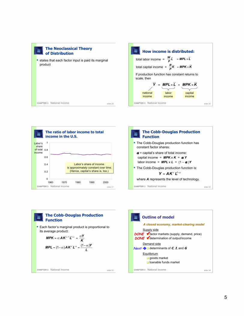
CHAPTER 3 National Income slide 48
EXERCISE:
Calculate the change in saving
Suppose MPC = 0.8 and MPL = 20.For each of the following, compute ΔS :
a. ΔG = 100b. ΔT = 100c. ΔY = 100d. ΔL = 10
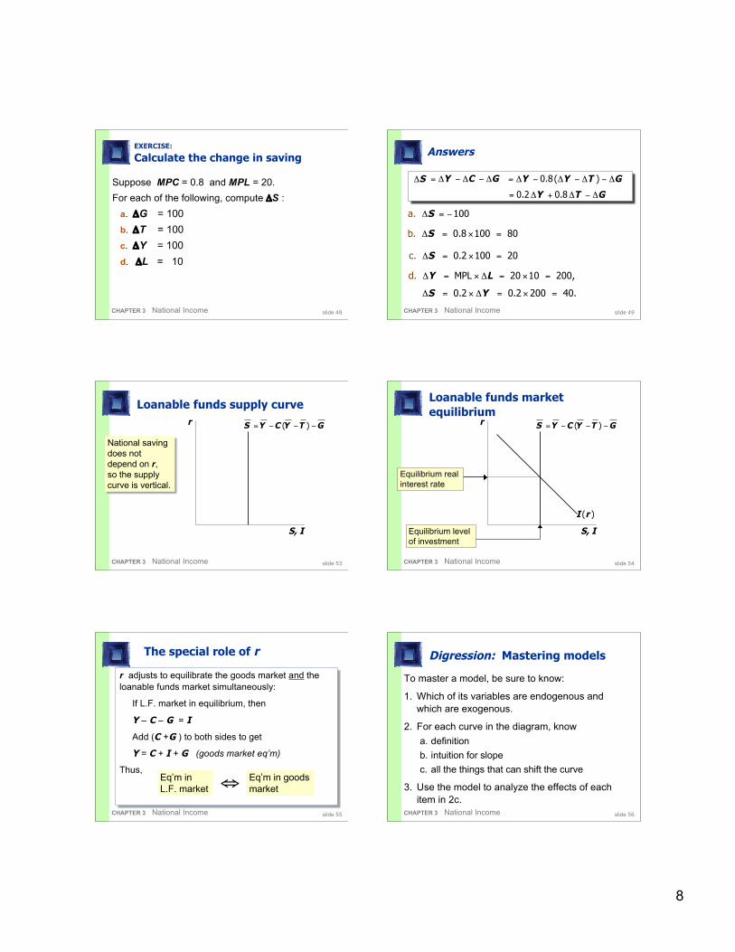
CHAPTER 3 National Income slide 49
Answers
S! 0.8( )Y Y T G= ! " ! " ! " !
0.2 0.8Y T G= ! + ! " !
1. 0a 0S! = "
0.8 0 0b. 10 8S! = " =
0.2 0 0c. 10 2S! = " =
MPL 20 10 20 ,d. 0Y L! = " ! = " =
0.2 0.2 200 40.S Y! = " ! = " =
Y C G= ! " ! " !
CHAPTER 3 National Income slide 53
Loanable funds supply curver
S, I
( )S Y C Y T G= ! ! !
National savingdoes notdepend on r,so the supplycurve is vertical.
CHAPTER 3 National Income slide 54
Loanable funds marketequilibrium
r
S, I
I (r )
( )S Y C Y T G= ! ! !
Equilibrium realinterest rate
Equilibrium levelof investment
CHAPTER 3 National Income slide 55
The special role of r
r adjusts to equilibrate the goods market and theloanable funds market simultaneously:
If L.F. market in equilibrium, then
Y – C – G = I
Add (C +G ) to both sides to get
Y = C + I + G (goods market eq’m)
Thus,Eq’m inL.F. market
Eq’m in goodsmarket!
CHAPTER 3 National Income slide 56
Digression: Mastering models
To master a model, be sure to know:
1. Which of its variables are endogenous andwhich are exogenous.
2. For each curve in the diagram, knowa. definitionb. intuition for slopec. all the things that can shift the curve
3. Use the model to analyze the effects of eachitem in 2c.

9
CHAPTER 3 National Income slide 57
Mastering the loanable fundsmodel
Things that shift the saving curve public saving
fiscal policy: changes in G or T private saving
preferences tax laws that affect saving
–401(k)– IRA–replace income tax with consumption tax
CHAPTER 3 National Income slide 58
CASE STUDY:The Reagan deficits
Reagan policies during early 1980s: increases in defense spending: ΔG > 0 big tax cuts: ΔT < 0
Both policies reduce national saving:
( )S Y C Y T G= ! ! !
G S! " # T C S! " # " !
CHAPTER 3 National Income slide 59
CASE STUDY:The Reagan deficits
r
S, I
1S
I (r )
r1
I1
r22. …which causes
the real interestrate to rise…
I2
3. …which reducesthe level ofinvestment.
1. The increase inthe deficitreduces saving…
2S
CHAPTER 3 National Income slide 60
Are the data consistent with these results?
variable 1970s 1980s
T – G –2.2 –3.9
S 19.6 17.4
r 1.1 6.3
I 19.9 19.4
T–G, S, and I are expressed as a percent of GDPAll figures are averages over the decade shown.
CHAPTER 3 National Income slide 62
Mastering the loanable fundsmodel, continued
Things that shift the investment curve some technological innovations
to take advantage of the innovation,firms must buy new investment goods
tax laws that affect investment investment tax credit
CHAPTER 3 National Income slide 63
An increase in investment demand
An increasein desiredinvestment…
r
S, I
I1
S
I2
r1
r2
…raises theinterest rate.
But the equilibriumlevel of investmentcannot increasebecause thesupply of loanablefunds is fixed.

10
Chapter SummaryChapter Summary
Total output is determined by the economy’s quantities of capital and labor the level of technology
Competitive firms hire each factor until itsmarginal product equals its price.
If the production function has constant returns toscale, then labor income plus capital incomeequals total income (output).
CHAPTER 3 National Income slide 66
Chapter SummaryChapter Summary
A closed economy’s output is used for consumption investment government spending
The real interest rate adjusts to equatethe demand for and supply of goods and services loanable funds
CHAPTER 3 National Income slide 67
Chapter SummaryChapter Summary
A decrease in national saving causes the interestrate to rise and investment to fall.
An increase in investment demand causes theinterest rate to rise, but does not affect theequilibrium level of investmentif the supply of loanable funds is fixed.
CHAPTER 3 National Income slide 68