M ACROECONOMICS C H A P T E R M ACROECONOMICS National Income: Where it Comes From and Where it Goes 3

MMACROECONOMICSACROECONOMICS

C H A P T E R

MMACROECONOMICSACROECONOMICS

National Income:Where it Comes From and Where it Goes

3

slide 2CHAPTER 3 National Income

Outline of model

A closed economy, market-clearing model

Supply side factor markets (supply, demand, price) determination of output/income

Demand side determinants of C, I, and G

Equilibrium goods market loanable funds market


Factors of production

K = capital: tools, machines, and structures used in production

L = labor: the physical and mental efforts of workers


The production function

denoted Y = F(K, L)

shows how much output (Y ) the economy can produce fromK units of capital and L units of labor

reflects the economy’s level of technology

exhibits constant returns to scale


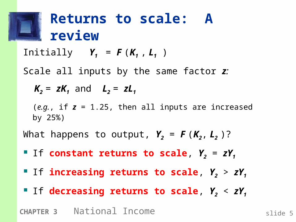
Returns to scale: A review

Initially Y1 = F (K1 , L1 )

Scale all inputs by the same factor z:

K2 = zK1 and L2 = zL1

(e.g., if z = 1.25, then all inputs are increased by 25%)

What happens to output, Y2 = F (K2, L2 )?

If constant returns to scale, Y2 = zY1

If increasing returns to scale, Y2 > zY1

If decreasing returns to scale, Y2 < zY1


try…

Determine whether constant, decreasing, or increasing returns to scale for each of these production functions:

(a)

(b) ( , )F K L K L

( , )K

F K LL

2


Assumptions of the model

1. Technology is fixed.

2. The economy’s supplies of capital and labor are fixed at

and K K L L


Determining GDP

Output is determined by the fixed factor supplies and the fixed state of technology:

, ( )Y F K L


The distribution of national income

determined by factor prices, the prices per unit that firms pay for the factors of production

wage = price of L

rental rate = price of K


Notation

W = nominal wage

R = nominal rental rate

P = price of output

W /P = real wage (measured in units of output)

R /P = real rental rate

W = nominal wage

R = nominal rental rate

P = price of output

W /P = real wage (measured in units of output)

R /P = real rental rate


How factor prices are determined

Factor prices are determined by supply and demand in factor markets.

Recall: Supply of each factor is fixed.

What about demand?


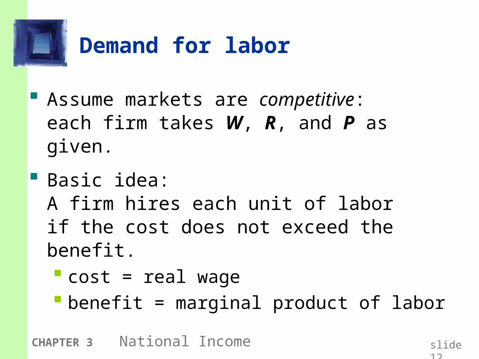
Demand for labor

Assume markets are competitive: each firm takes W, R, and P as given.

Basic idea:A firm hires each unit of labor if the cost does not exceed the benefit. cost = real wage benefit = marginal product of labor


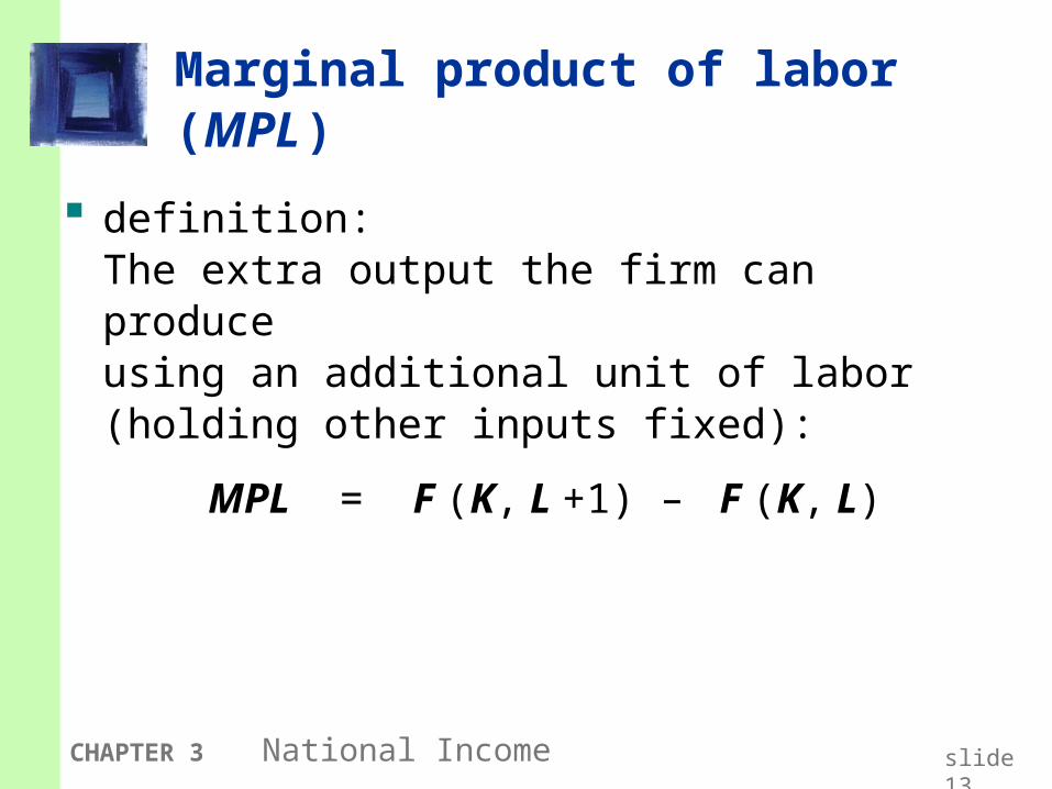
Marginal product of labor (MPL )

definition:The extra output the firm can produce using an additional unit of labor (holding other inputs fixed):

MPL = F (K, L +1) – F (K, L)


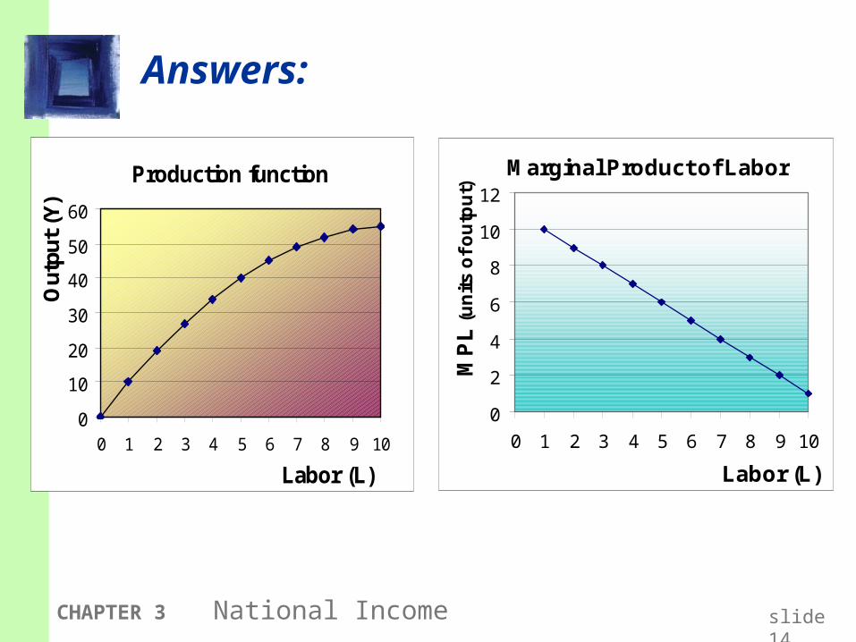
Answers:

Production function

0

10

20

30

40

50

60

0 1 2 3 4 5 6 7 8 9 10

Labor (L)

Out

put

(Y)

Marginal Product of Labor

0

2

4

6

8

10

12

0 1 2 3 4 5 6 7 8 9 10

Labor (L)M

PL

(u

nit

s o

f o

utp

ut)


Youtput

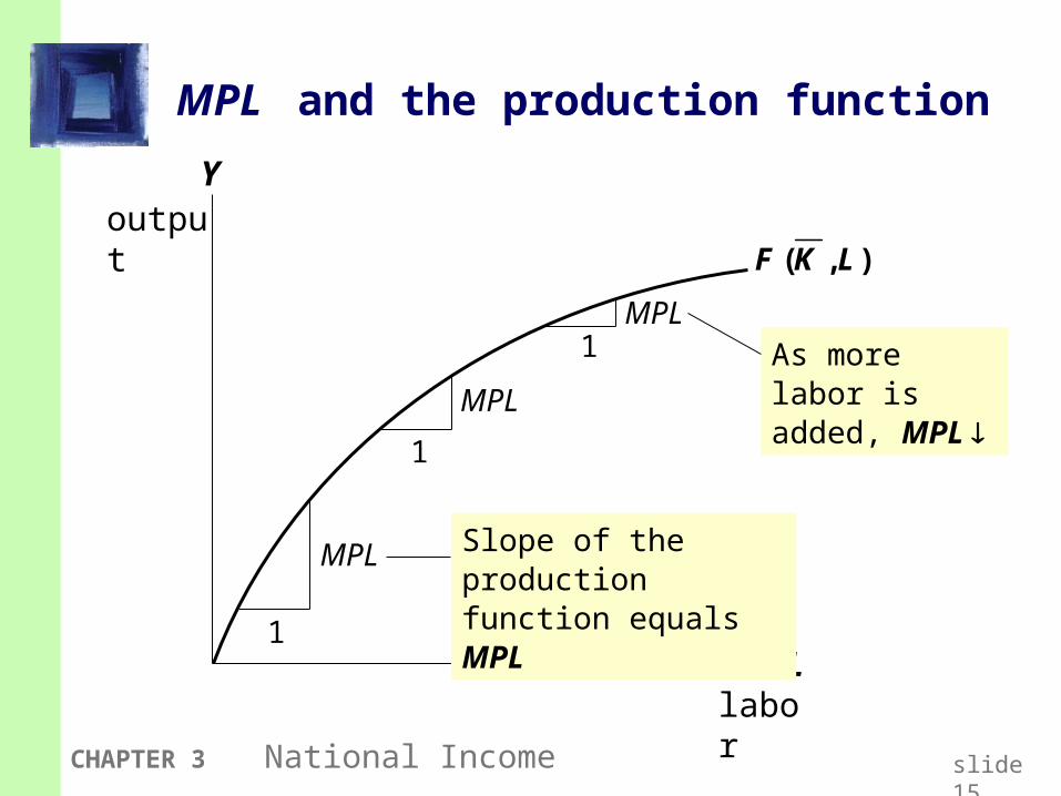
MPL and the production function

Llabor

F K L( , )

1

MPL

1

MPL

1MPL As more labor

is added, MPL

Slope of the production function equals MPL


Diminishing marginal returns

As a factor input is increased, its marginal product falls (other things equal).

Intuition:Suppose L while holding K fixed

fewer machines per worker

lower worker productivity


MPL and the demand for labor

Each firm hires labor up to the point where MPL = W/P.

Each firm hires labor up to the point where MPL = W/P.

Units of output

Units of labor, L

MPL, Labor demand

Real wage

Quantity of labor demanded


The equilibrium real wage

The real wage adjusts to equate labor demand with supply.

The real wage adjusts to equate labor demand with supply.

Units of output

Units of labor, L

MPL, Labor demand

equilibrium real wage

Labor supply

L


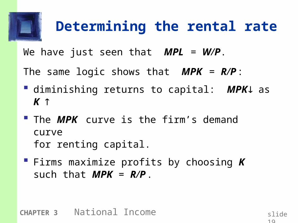
Determining the rental rate

We have just seen that MPL = W/P.

The same logic shows that MPK = R/P :

diminishing returns to capital: MPK as K

The MPK curve is the firm’s demand curve for renting capital.

Firms maximize profits by choosing K

such that MPK = R/P .


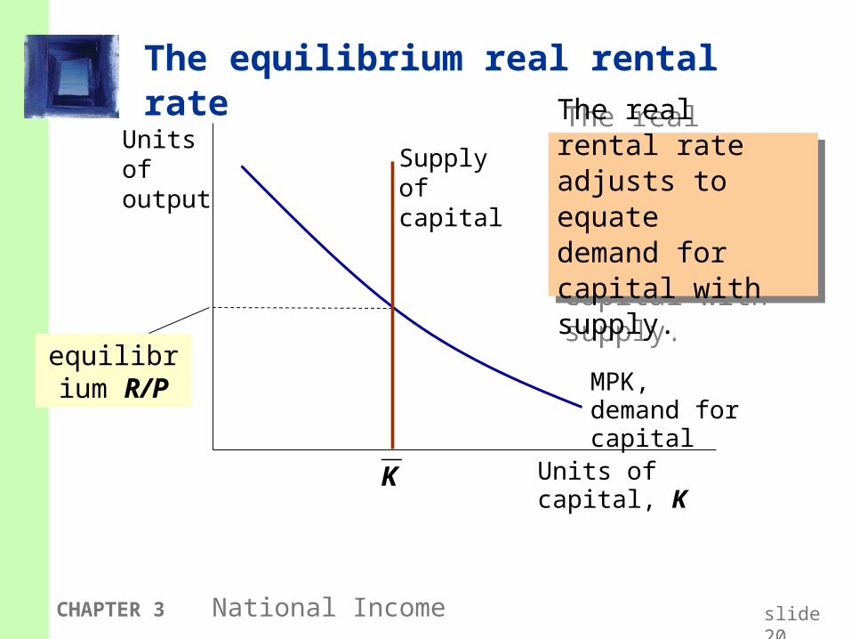
The equilibrium real rental rate

The real rental rate adjusts to equate demand for capital with supply.

The real rental rate adjusts to equate demand for capital with supply.

Units of output

Units of capital, K

MPK, demand for capital

equilibrium R/P

Supply of capital

K


The Neoclassical Theory of Distribution

states that each factor input is paid its marginal product

is accepted by most economists


How income is distributed:

total labor income =

If production function has constant returns to scale, then

total capital income =

WL

PMPL L

RK

PMPK K

Y MPL L MPK K

laborincome

capitalincome

nationalincome


The ratio of labor income to total income in the U.S.

0

0.2

0.4

0.6

0.8

1

1960 1970 1980 1990 2000

Labor’s share

of total income

Labor’s share of income is approximately constant over time.

(Hence, capital’s share is, too.)

Labor’s share of income is approximately constant over time.

(Hence, capital’s share is, too.)


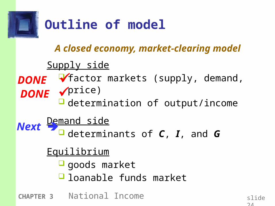
Outline of model

A closed economy, market-clearing model

Supply side factor markets (supply, demand, price) determination of output/income

Demand side determinants of C, I, and G

Equilibrium goods market loanable funds market

DONE DONE

Next


Demand for goods & services

Components of aggregate demand:

C = consumer demand for g & s

I = demand for investment goods

G = government demand for g & s

(closed economy: no NX )


Consumption, C

def: Disposable income is total income minus total taxes: Y – T.

Consumption function: C = C (Y – T )Shows that (Y – T ) C

def: Marginal propensity to consume (MPC) is the increase in C caused by a one-unit increase in disposable income.


The consumption function

C

Y – T

C (Y –T )

1

MPCThe slope of the consumption function is the MPC.


Investment, I

The investment function is I = I (r ),

where r denotes the real interest rate, the nominal interest rate corrected for inflation.

The real interest rate is the cost of borrowing the opportunity cost of using one’s own

funds to finance investment spending.

So, r I


The investment function

r

I

I

(r )

Spending on investment goods depends negatively on the real interest rate.


Government spending, G

G = govt spending on goods and services.

G excludes transfer payments (e.g., social security benefits, unemployment insurance benefits).

Assume government spending and total taxes are exogenous:

and G G T T


The market for goods & services

Aggregate demand:

Aggregate supply:

Equilibrium:

The real interest rate adjusts to equate demand with supply.

( ) ( )C Y T I r G

( , )Y F K L

= ( ) ( )Y C Y T I r G


The loanable funds market

A simple supply-demand model of the financial system.

One asset: “loanable funds” demand for funds: investment supply of funds: saving “price” of funds: real interest rate


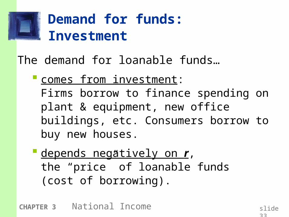
Demand for funds: Investment

The demand for loanable funds…

comes from investment:Firms borrow to finance spending on plant & equipment, new office buildings, etc. Consumers borrow to buy new houses.

depends negatively on r, the “price” of loanable funds (cost of borrowing).


Loanable funds demand curve

r

I

I

(r )

The investment curve is also the demand curve for loanable funds.

The investment curve is also the demand curve for loanable funds.


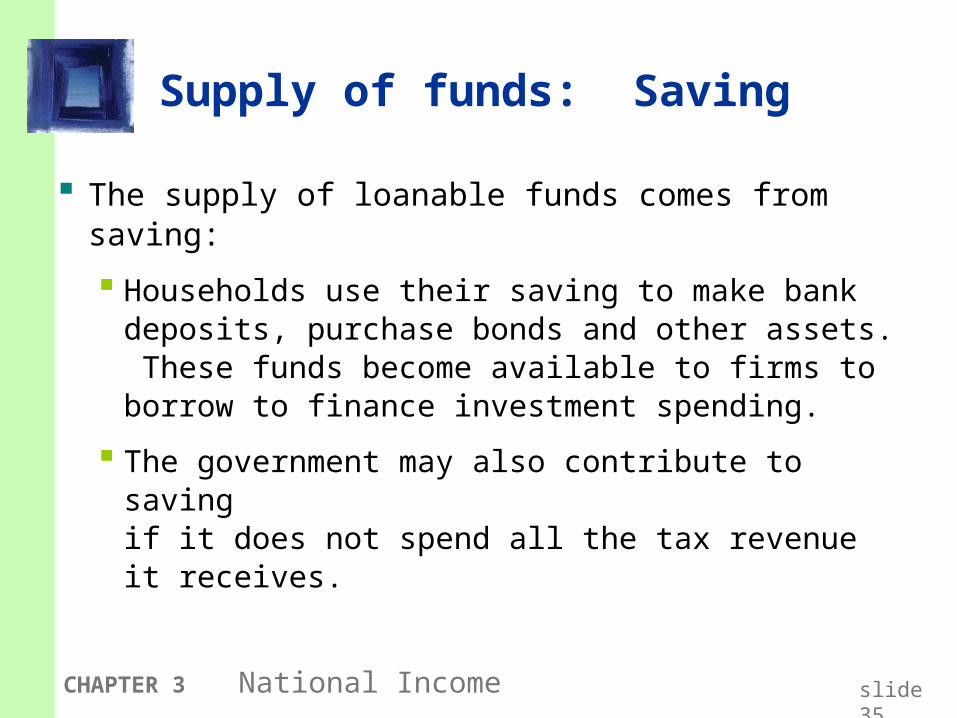
Supply of funds: Saving

The supply of loanable funds comes from saving:

Households use their saving to make bank deposits, purchase bonds and other assets. These funds become available to firms to borrow to finance investment spending.

The government may also contribute to saving if it does not spend all the tax revenue it receives.


Types of saving

private saving = (Y – T ) – C

public saving = T – G

national saving, S

= private saving + public saving

= (Y –T ) – C + T – G

= Y – C – G


EXERCISE:

Calculate the change in saving

Suppose MPC = 0.8 and MPL = 20.

For each of the following, compute S :

a. G = 100

b. T = 100

c. Y = 100

d. L = 10


Answers

S 0.8( )Y Y T G

0.2 0.8Y T G

1. 0a 0S

0.8 0 0b. 10 8S

0.2 0 0c. 10 2S

MPL 20 10 20 ,d. 0Y L

0.2 0.2 200 40.S Y

Y C G


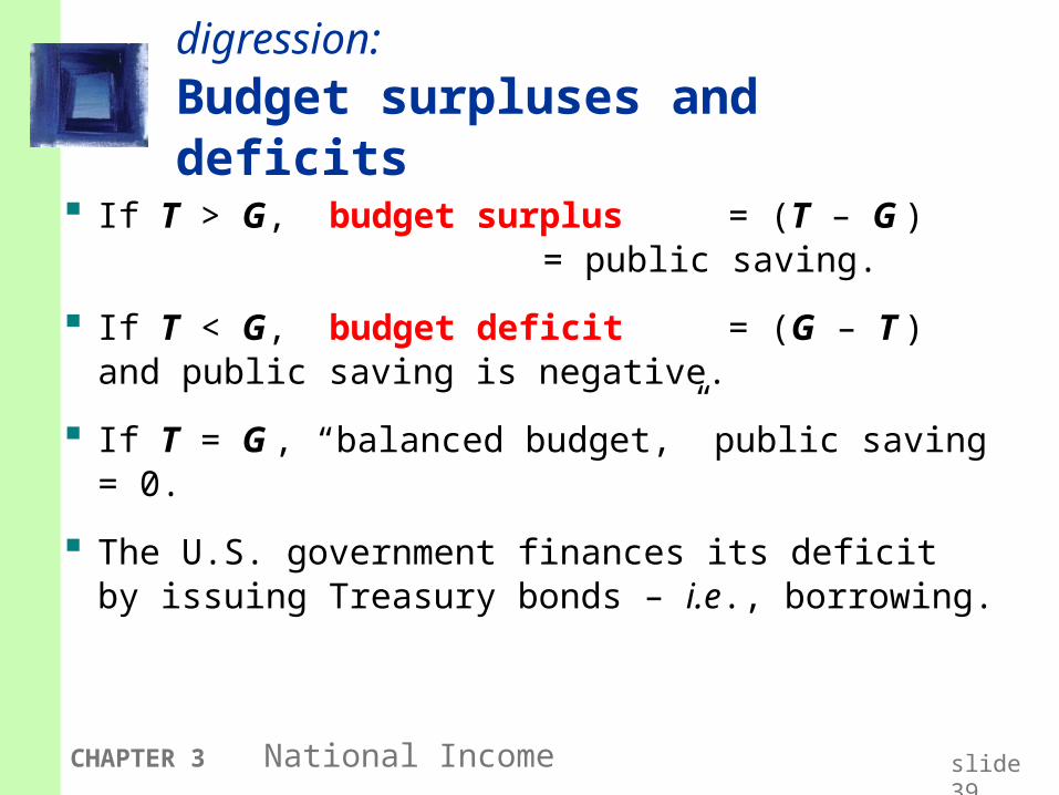
digression: Budget surpluses and deficits

If T > G, budget surplus = (T – G ) = public saving.

If T < G, budget deficit = (G – T )and public saving is negative.

If T = G , “balanced budget,” public saving = 0.

The U.S. government finances its deficit by issuing Treasury bonds – i.e., borrowing.


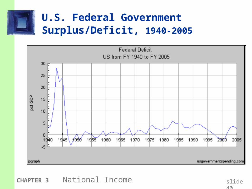
U.S. Federal Government Surplus/Deficit, 1940-2005


U.S. Federal Government Surplus/Deficit, 1940-2011


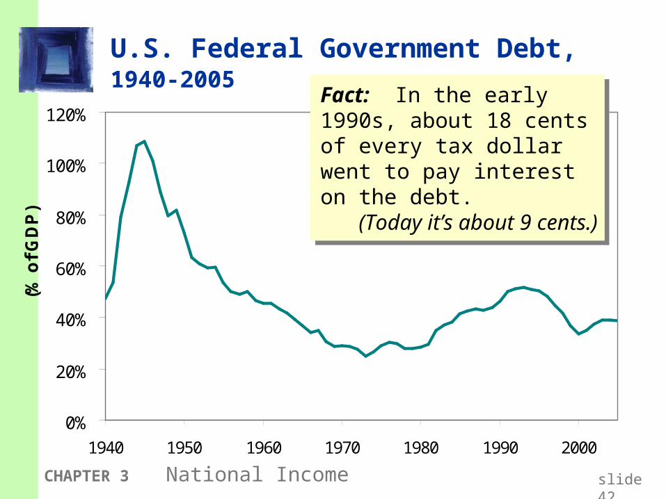
U.S. Federal Government Debt, 1940-2005

0%

20%

40%

60%

80%

100%

120%

1940 1950 1960 1970 1980 1990 2000

(% o

f G

DP

)

Fact: In the early 1990s, about 18 cents of every tax dollar went to pay interest on the debt. (Today it’s about 9 cents.)

Fact: In the early 1990s, about 18 cents of every tax dollar went to pay interest on the debt. (Today it’s about 9 cents.)


Loanable funds supply curver

S, I

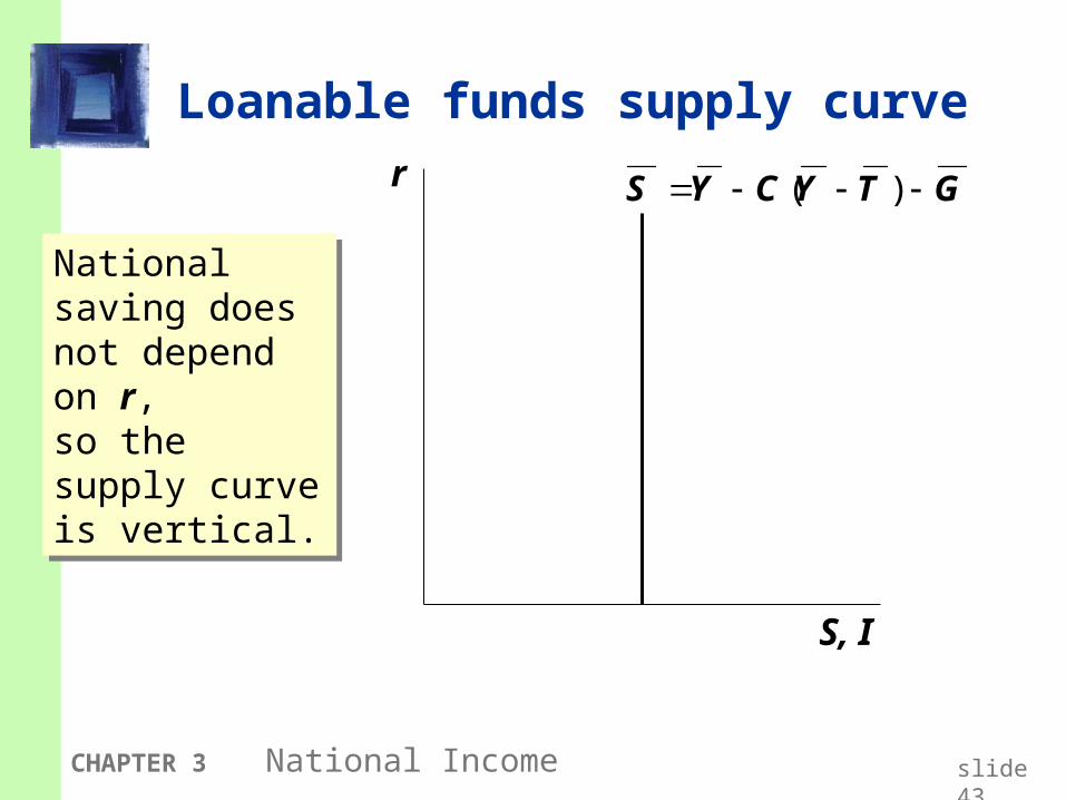
( )S Y C Y T G

National saving does not depend on r, so the supply curve is vertical.

National saving does not depend on r, so the supply curve is vertical.


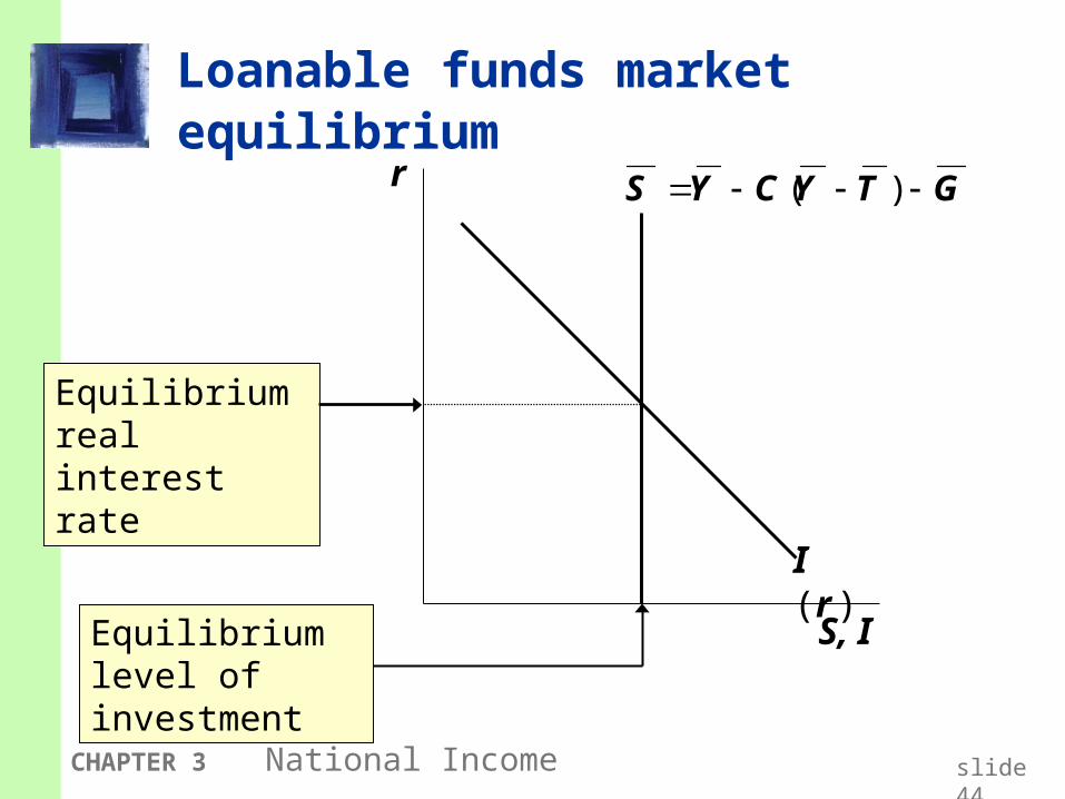
Loanable funds market equilibrium

r

S, I

I (r )

( )S Y C Y T G

Equilibrium real interest rate

Equilibrium level of investment


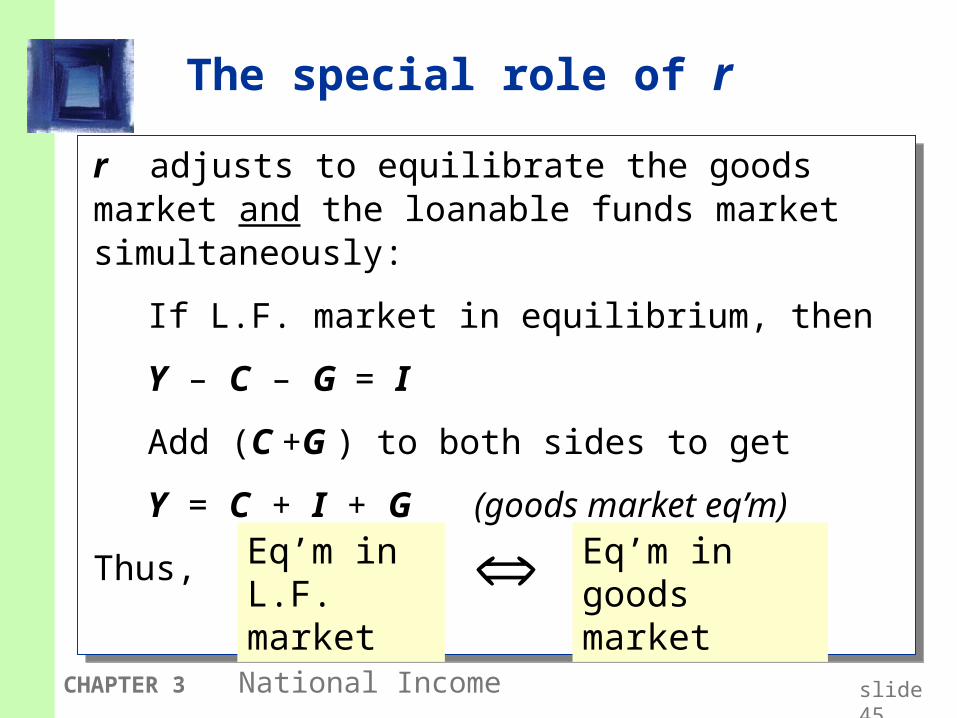
The special role of r

r adjusts to equilibrate the goods market and the loanable funds market simultaneously:

If L.F. market in equilibrium, then

Y – C – G = I

Add (C +G ) to both sides to get

Y = C + I + G (goods market eq’m)

Thus,

r adjusts to equilibrate the goods market and the loanable funds market simultaneously:

If L.F. market in equilibrium, then

Y – C – G = I

Add (C +G ) to both sides to get

Y = C + I + G (goods market eq’m)

Thus, Eq’m in L.F. market

Eq’m in goods market


Digression: Mastering models

To master a model, be sure to know:

1. Which of its variables are endogenous and which are exogenous.

2. For each curve in the diagram, know

a. definition

b. intuition for slope

c. all the things that can shift the curve

3. Use the model to analyze the effects of each item in 2c.


Mastering the loanable funds model

Things that shift the saving curve public saving

fiscal policy: changes in G or T private saving

preferences tax laws that affect saving

–401(k)

– IRA

–replace income tax with consumption tax


CASE STUDY: The Reagan deficits

Reagan policies during early 1980s: increases in defense spending: G > 0 big tax cuts: T < 0

Both policies reduce national saving:

( )S Y C Y T G

G S T C S


CASE STUDY: The Reagan deficits

r

S, I

1S

I (r )

r1

I1

r2

2. …which causes the real interest rate to rise…

2. …which causes the real interest rate to rise…

I2

3. …which reduces the level of investment.

3. …which reduces the level of investment.

1. The increase in the deficit reduces saving…

1. The increase in the deficit reduces saving…

2S


Mastering the loanable funds model, continued

Things that shift the investment curve

some technological innovations

to take advantage of the innovation, firms must buy new investment goods

tax laws that affect investment

investment tax credit


An increase in investment demand

An increase in desired investment…

r

S, I

I1

S

I2

r1

r2

…raises the interest rate.

But the equilibrium level of investment cannot increase because thesupply of loanable funds is fixed.


Saving and the interest rate

Why might saving depend on r ?

How would the results of an increase in investment demand be different?

Would r rise as much?

Would the equilibrium value of I change?


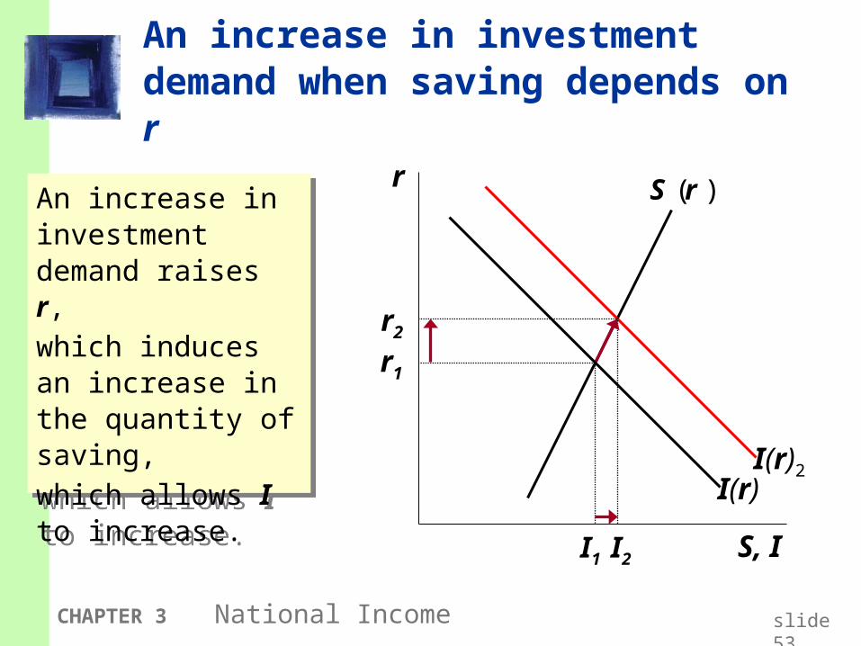
An increase in investment demand when saving depends on r

r

S, I

I(r)

( )S r

I(r)2

r1

r2

An increase in investment demand raises r, which induces an increase in the quantity of saving,which allows I to increase.

An increase in investment demand raises r, which induces an increase in the quantity of saving,which allows I to increase.

I1 I2

Chapter SummaryChapter Summary

Total output is determined by the economy’s quantities of capital and labor the level of technology

Competitive firms hire each factor until its marginal product equals its price.

If the production function has constant returns to scale, then labor income plus capital income equals total income (output).

CHAPTER 3 National Income slide 54


A closed economy’s output is used for consumption investment government spending

The real interest rate adjusts to equate the demand for and supply of goods and services loanable funds



A decrease in national saving causes the interest rate to rise and investment to fall.

An increase in investment demand causes the interest rate to rise, but does not affect the equilibrium level of investment if the supply of loanable funds is fixed.


slide 57CHAPTER 4 Money and Inflation

In this chapter, you will learn…

The classical theory of inflation causes effects social costs

“Classical” – assumes prices are flexible & markets clear

Applies to the long run

slide 58

U.S. inflation and its trend, 1960-2007

slide 58

0%

3%

6%

9%

12%

15%

1960 1965 1970 1975 1980 1985 1990 1995 2000 2005

long-run trend

% change in CPI from 12 months earlier


The connection between money and prices

Inflation rate = the percentage increase in the average level of prices.

Price = amount of money required to buy a good.

Because prices are defined in terms of money, we need to consider the nature of money, the supply of money, and how it is controlled.


Money: Definition

MoneyMoney is the stock is the stock of assets that can be of assets that can be readily used to make readily used to make

transactions.transactions.


Money: Functions

medium of exchangewe use it to buy stuff

store of valuetransfers purchasing power from the present to the future

unit of accountthe common unit by which everyone measures prices and values


Money: Types

1. fiat money has no intrinsic value example: the paper currency we use

2. commodity money has intrinsic value examples:

gold coins, cigarettes in P.O.W. camps


The money supply and monetary policy definitions

The money supply is the quantity of money available in the economy.

Monetary policy is the control over the money supply.


The central bank

Monetary policy is conducted by a country’s central bank.

In the U.S., the central bank is called the Federal Reserve (“the Fed”).

The Federal Reserve Building Washington, DC


Money supply measures, May 2007

$7227

M1 + small time deposits, savings deposits, money market mutual funds, money market deposit accounts

M2

$1377C + demand deposits, travelers’ checks, other checkable deposits

M1

$755CurrencyC

amount ($ billions)

assets includedsymbol


The Quantity Theory of Money

A simple theory linking the inflation rate to the growth rate of the money supply.

Begins with the concept of velocity…


Velocity

basic concept: the rate at which money circulates

definition: the number of times the average dollar bill changes hands in a given time period

example: In 2007, $500 billion in transactions money supply = $100 billion The average dollar is used in five transactions

in 2007 So, velocity = 5


Velocity, cont.

This suggests the following definition:

TV

M

where

V = velocity

T = value of all transactions

M = money supply


Velocity, cont.

Use nominal GDP as a proxy for total transactions.

Then, P YV

M

where

P = price of output (GDP

deflator)

Y = quantity of output (real GDP)

P Y = value of output (nominal

GDP)


The quantity equation

The quantity equationM V = P Y

follows from the preceding definition of velocity.

It is an identity: it holds by definition of the variables.


Money demand and the quantity equation

M/P = real money balances, the purchasing power of the money supply.

A simple money demand function: (M/P )d = k Y

wherek = how much money people wish to hold for each dollar of income. (k is exogenous)


Money demand and the quantity equation

money demand: (M/P )d = k Y

quantity equation: M V = P Y

The connection between them: k = 1/V

When people hold lots of money relative to their incomes (k is high), money changes hands infrequently (V is low).


Back to the quantity theory of money

starts with quantity equation

assumes V is constant & exogenous:

With this assumption, the quantity equation can be written as

V V

M V P Y


The quantity theory of money, cont.

How the price level is determined:

With V constant, the money supply determines nominal GDP (P Y ).

Real GDP is determined by the economy’s supplies of K and L and the production function (Chap 3).

The price level is P = (nominal GDP)/(real GDP).

M V P Y



Recall from Chapter 2: The growth rate of a product equals the sum of the growth rates.

The quantity equation in growth rates:

M V P YM V P Y

The quantity theory of money assumes

is constant, so = 0.V

VV



(Greek letter “pi”) denotes the inflation rate:

M P YM P Y

PP

The result from the preceding slide was:

Solve this result for to get



Normal economic growth requires a certain amount of money supply growth to facilitate the growth in transactions.

Money growth in excess of this amount leads to inflation.



Y/Y depends on growth in the factors of production and on technological progress (all of which we take as given, for now).

Hence, the Quantity Theory predicts Hence, the Quantity Theory predicts

a one-for-one relation between a one-for-one relation between

changes in the money growth rate and changes in the money growth rate and

changes in the inflation rate. changes in the inflation rate.

Hence, the Quantity Theory predicts Hence, the Quantity Theory predicts

a one-for-one relation between a one-for-one relation between

changes in the money growth rate and changes in the money growth rate and

changes in the inflation rate. changes in the inflation rate.


Confronting the quantity theory with data

The quantity theory of money implies

1. countries with higher money growth rates should have higher inflation rates.

2. the long-run trend behavior of a country’s inflation should be similar to the long-run trend in the country’s money growth rate.

Are the data consistent with these implications?

slide 80

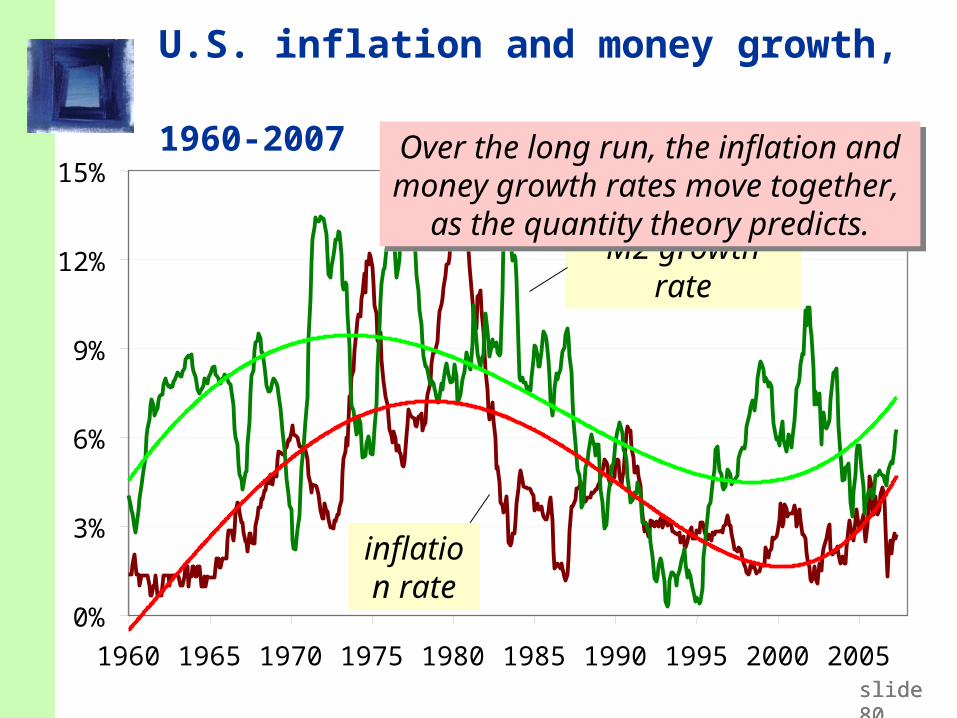
U.S. inflation and money growth, 1960-2007

slide 80

0%

3%

6%

9%

12%

15%

1960 1965 1970 1975 1980 1985 1990 1995 2000 2005

inflation rate

M2 growth rate

Over the long run, the inflation and money growth rates move together,

as the quantity theory predicts.

Over the long run, the inflation and money growth rates move together,

as the quantity theory predicts.


Seigniorage

To spend more without raising taxes or selling bonds, the govt can print money.

The “revenue” raised from printing money is called seigniorage (pronounced SEEN-your-idge).

The inflation tax:Printing money to raise revenue causes inflation. Inflation is like a tax on people who hold money.


Inflation and interest rates

Nominal interest rate, inot adjusted for inflation

Real interest rate, radjusted for inflation:

r = i


The Fisher effect

The Fisher equation: i = r +

Chap 3: S = I determines r .

Hence, an increase in causes an equal increase in i.

This one-for-one relationship is called the Fisher effect.

slide 84

Inflation and nominal interest rates in the U.S., 1955-2007

percent per year

slide 84

inflation rate

nominal interest rate

-3%

0%

3%

6%

9%

12%

15%

1955 1960 1965 1970 1975 1980 1985 1990 1995 2000 2005

Documents

M ACROECONOMICS C H A P T E R M ACROECONOMICS National Income: Where it Comes From and Where it Goes 3