Embed Size (px)
Citation preview

Accelerated Whole-Brain Multi-Parameter Mapping using Blind Compressed Sensing
Sampada Bhave†, Sajan Goud Lingala§, Casey P. Johnson‡, Vincent A. Magnotta‡, Mathews Jacob†
†Department of Electrical and Computer Engineering, The University of Iowa, Iowa
‡Department of Radiology, The University of Iowa, Iowa
§Department of Electrical Engineering, University of Southern California, California
March 12, 2015
Correspondence to :
Mathews Jacob
Department of Electrical and Computer Engineering
3314 Seamans Center
University of Iowa, IA 52242
Email: [email protected]
Phone: (319) 335-6420
This work is supported by grants NSF CCF-0844812, NSF CCF-1116067, NIH 1R21HL109710-01A1, ACS
RSG-11-267-01-CCE, and ONR N00014-13-1-0202.
Approximate word count : 4946
Number of figures & tables: 10
1

Abstract
Purpose: To introduce a blind compressed sensing (BCS) framework to accelerate multi-parameter MR
mapping, and demonstrate its feasibility in high-resolution, whole-brain T1ρ and T2 mapping.
Methods: BCS models the evolution of magnetization at every pixel as a sparse linear combination of
bases in a dictionary. Unlike compressed sensing (CS), the dictionary and the sparse coefficients are
jointly estimated from under-sampled data. Large number of non-orthogonal bases in BCS accounts for
more complex signals than low rank representations. The low degree of freedom of BCS, attributed to
sparse coefficients, translates to fewer artifacts at high acceleration factors(R).
Results: From 2D retrospective under-sampling experiments, the mean square errors in T1ρ and T2 maps
were observed to be within 0.1% up to R=10. BCS was observed to be more robust to patient-specific
motion as compared to other CS schemes and resulted in minimal degradation of parameter maps in the
presence of motion. Our results suggested that BCS can provide an acceleration factor of 8 in prospective
3D imaging with reasonable reconstructions.
Conclusion: BCS considerably reduces scan time for multi-parameter mapping of the whole brain with
minimal artifacts, and is more robust to motion-induced signal changes compared to current CS and PCA
based techniques.
Key words: T1ρ imaging, T2 imaging, dictionary learning, blind compressed sensing (BCS),
3D multi-parameter mapping
2

INTRODUCTION
The quantification of multiple tissue parameters from MRI datasets is emerging as a powerful tool for
tissue characterization (1–8). Parameters such as proton density, longitudinal and transverse relaxation
times (denoted by T1 and T2), relaxation times in the rotating frame (T1ρ and T2ρ ), as well as diffusion
have been shown to be useful in diagnosis of various diseases including cerebral ischemia (9), Parkinson’s
disease (2–4), Alzheimer’s disease (2, 5, 7), epilepsy (7) multiple sclerosis (6, 7), edema (8), necrosis (8),
liver fibrosis (10), and intervertebral disc and cartilage degeneration (11–13). Although a single parameter
may be sensitive to a number of tissue properties of interest, it may not be specific. Acquiring additional
parameters can improve the specificity. The main bottleneck in the routine clinical use of multi-parameter
mapping is the long scan time associated with the acquisition of MR images with multiple weightings or
contrast values. In addition, long scan times are likely to result in motion induced artifacts in the data.
A common approach to reduce the scan time is to limit the number of weighted images from which the
parameters are estimated. However, this approach precludes the use of multi-exponential fitting methods,
limits the accuracy of fits, and restrict the dynamic range of estimated tissue parameters. Several researchers
have proposed to accelerate the acquisition of the weighted images using parallel imaging, model-based
compressed sensing, and low-rank signal modeling (14–22). The use of parallel imaging alone can only
provide moderate acceleration factors (14). Model-based compressed sensing methods rely on large dictio-
naries generated by Bloch equation simulations of all possible parameter combinations (23). A challenge
associated with this scheme is its vulnerability to patient motion, mainly because the dictionary basis func-
tions cannot account for motion induced signal changes. Another problem with the direct application of this
scheme to multi-parameter imaging is the rapid growth in the size of the dictionaries with the number of
parameters, which also results in increased complexity of the non-linear recovery algorithm. In this context,
methods such as k-t PCA and PSF models that estimate the basis functions from the measured data itself are
more desirable; the basis functions can model motion induced signal changes and thus provide improved
recovery of weighted images (22, 24).
The main contribution of this paper is to optimize the blind compressed sensing (BCS) scheme, which
was originally introduced for dynamic imaging (25), to accelerate multi-parameter mapping. The BCS
scheme represents the evolution of the magnetization of the pixels as a sparse linear combination of basis
functions in a finite dictionary V. Specifically, the Casorati matrix of the data X is modeled as X = UV.
3

This model is ideally suited for multi-parameter mapping since there are finite number of distinct tissue types
in the specimen with unique parameter values. The proposed algorithm learns the dictionary basis functions,
as well as their sparse coefficients U, from the undersampled data by solving a constrained optimization
problem. The criterion is a linear combination of the data fidelity term and a sparsity promoting `1 norm
on the coefficient matrix U, subject to the Frobenius norm constraint on the dictionary V. Unlike methods
such as (26) that pre-estimate the dictionary, this approach provides robustness to patient-specific motion.
When the data is truly low-rank, the k-t PCA and PSF schemes (22, 24) requires very few basis functions to
represent it. However, in many cases (e.g. in the presence of motion, multiple tissue types, and simultaneous
mapping of multiple parameters), the rank of the dataset can be considerably higher; the larger degrees of
freedom will translate to a tradeoff between accuracy and artifacts, especially at high acceleration factors.
The BCS scheme uses a considerably larger dictionary of non-orthogonal basis functions, which provides
a richer representation of the data compared to the smaller dictionary of orthogonal basis functions used
in the k-t PCA and PSF schemes. The sparsity of the coefficients ensures that the number of active basis
functions at each voxel are considerably lower than the rank of the dataset. Since the basis functions used
at different spatial locations are different, the BCS scheme can be viewed as a locally low-rank scheme; the
appropriate basis functions (subspace) at each voxel are selected independently. Since the number of basis
functions required at each voxel is considerably lower than the global rank, the BCS scheme can provide
a richer representation with lower degrees of freedom; this translates to better trade-offs between accuracy
and achievable acceleration, especially in multi-parametric datasets with inter-frame motion.
The BCS algorithm (25) was inspired by the theoretical work on BCS by Gleichman et al. (27). The
work by Gleichman et. al. considers the same sensing matrix for all time frames, for simplicity of the
derivations. The proposed scheme uses different sensing matrices for different frames. The experiments in
(25, 28) clearly demonstrate the benefit of higher spatial and temporal incoherency offered by this sampling
strategy. In addition, the algorithm used in (27) is fundamentally different from our setting. The proposed
scheme is also motivated by and have similarities to the partial separable function (PSF) model introduced
by Liang et al. (16, 24, 29). However, there are several key differences between the PSF implementations
and the proposed scheme. For example, (24) uses the power factorization method to exploit the low-rank
structure of X. They jointly estimate U and V by alternating between two quadratic optimization schemes
involving data consistency terms. Our previous work shows that the BCS scheme provides improved re-
constructions than low-rank methods, including power-factorization (24, 25), mainly because of the richer
4

dictionary and the lower degrees of freedom. Zhao et. al, assumes the data to be low-rank and pre-estimates
the orthogonal basis set V from low resolution data (29); they then estimate the coefficients using a sparsity
penalty on U. This approach can be seen as the first step of our iterative algorithm to jointly estimate U
and V. Specifically, the joint estimation of U and V will provide a richer dictionary with non-orthogonal
basis functions, which provide sparser coefficients than the orthogonal basis functions in (29). This is not
unexpected since extensive work in image processing have shown that over-complete and non-orthogonal
dictionaries/frames offer more compact representations than orthogonal basis sets. The comparisons in Fig.
4 demonstrate the performance improvement offered by the proposed joint estimation scheme.
We study the utility of the proposed BCS scheme to simultaneously recover T1ρ and T2 maps from
under-sampled weighted images. We rely on Cartesian sub-sampling schemes. The proposed scheme
yields reasonable estimates from the whole-brain for eight fold under-sampling over the fully-sampled setup,
thereby reducing the scan time to 20 min.
METHODS
In a multi-parameter imaging, the k-space data corresponding to different image contrasts are often sequen-
tially acquired by manipulating the sequence parameters (e.g. echo time, spin lock duration/amplitude and
flip angle). We denote the parametric dimension by p. The multi-coil under-sampled acquisition of such an
experiment is modeled as:
b(k, p) = A [γ(x, p)] + n(k, p), [1]
where b(k, t) represents the concatenated vector of the k− p measurements from all the coils. γ(x, p)(x =
(x1, y1)) denotes the underlying images pertaining to different contrasts; and n is additive noise. A is the
operator that models coil sensitivity and Fourier encoding on a specified k− p sampling trajectory.
Blind compressed sensing (BCS) formulation
The BCS model relies on the assumption that there exists a finite number of distinct tissue types with
unique relaxation parameter values within the specimen of interest; the evolution of the magnetization of
the tissue types as a function of p can be represented efficiently as a linear combination of basis functions
in a dictionary VR×N . Here R denotes the total number of basis functions in the dictionary and N is the
5
total number of contrast weighted images in the dataset. The signal evolution at the pixel specified by x is
modeled as a sparse linear combination of basis functions vi(p); i = 1, ..R in V (Also see Fig 1.):
γ(x, p) =R∑i=1
ui(x)︸ ︷︷ ︸sparse spatial weights
vi(p)︸ ︷︷ ︸learned bases
. [2]
Using the Casorati matrix notation (16), the above equation can be rewritten as
ΓM×N =
γ(x1, p1) . γ(x1, pN )
. . .
. . .
γ(xM , p1) . γ(xM , pN )
= UM×R VR×N , [3]
where M is the total number of pixels in the image, ui(x) and vi(p) in Eq. [2] are respectively the ith
column and row entries of U,V. We formulate the joint recovery of U,V from under-sampled multi-coil
k − p measurements as the following constrained minimization problem:
{U∗,V∗} = arg minU,V
‖A(UV)− b‖2F + λ‖U‖l1︸ ︷︷ ︸C(U,V)
such that ‖V‖2F < 1. [4]
The first term in Eq. [4] ensures data consistency. The second term promotes sparsity on the spatial coeffi-
cients ui(x) by utilizing a convex `1 norm prior on U, which is given by ‖U‖l1 =(∑M
i=1
∑rj=1 |u(i, j)|
),
and λ is the regularization parameter. The optimization problem is constrained by imposing unit Frobenius
norm on the over-complete dictionary V, making the recovery problem well posed. Note that we are jointly
estimating the sparse coefficients U and the subject-specific dictionary V directly from the under-sampled
k − p data. Since the dictionary is subject-specific, this approach ensures that any deviations from the true
parametric encoding, such as subject motion, field inhomogeneity and chemical shift artifacts, are learned
by the basis functions. The number of active bases at a specified voxel depends on several factors that in-
clude partial volume effects, motion, and magnetization disturbances due to inhomogeneity artifacts. The
spatial weights ui(x) are encouraged to be sparse since we expect only a few tissue types to be active at
any specified voxel. The main difference of the proposed implementation from (25) is the use of an efficient
algorithm and the extension to multi-coil formulation which enables better recovery at high acceleration
rates.
6

Optimization Algorithm
We majorize an approximation of the `1 penalty on U in (4) as ‖U‖`1 ≈ minLβ2 ‖U−L‖2 + ‖L‖`1 , where
L is an auxiliary variable. This approximation becomes exact as β →∞. When β is small, the majorization
is equivalent to the Frobenius norm on U (30). We use a variable splitting and augmented Lagrangian
optimization scheme to enforce the constraint in Eq. [4]. Thus, the optimization problem corresponds to
{U∗,V∗} = arg minU,V
minQ,L‖A(UV)− b‖2F +
β
2‖U− L‖2 + λ‖L‖l1 such that ‖Q‖2F < 1,V = Q [5]
Here, Q is the auxiliary variable for V. The constraint V = Q is enforced by adding the augmented
Lagrangian term α2 ‖V−Q‖2+〈Λ, (V −Q)〉 to the above cost function. Here, Λ is the Lagrange multiplier
term that will enforce the constraint. These simplifications enable us to decouple the optimization problem
in (4) into different sub-problems. We use an alternating strategy to solve for the variables U,V,Q and L.
All of these sub-problems are solved independently in an efficient fashion as described below, assuming the
other variables to be fixed.
Update on L: The sub-problem can be solved analytically as
Ln+1 =U|Un|
(|Un| −
1β
)+
[6]
where ‘+’ represents the soft thresholding operator defined as (τ)+ = max{0, τ} and β is the penalty
parameter.
Update on U: The sub-problem on U, assuming the other variables to be fixed, can be written as
Un+1 = arg minU
‖A(UnVn)− b‖22 +λβ
2‖U− Ln+1‖22 [7]
Since it is a quadratic problem, we solve it using a conjugate gradient (CG) algorithm. Here, Un, Vn and
Ln are the variables at the nth iteration.
Update on Q: This sub-problem, assuming the other variables to be fixed, is solved using a projection
scheme as specified in Eq. [8].
Qn+1 =
Vn when ‖Vn‖2F 6 1
1‖Vn‖F Vn else
[8]
7

Note that Qn is obtained by scaling Vn so that the Frobenius norm is unity.
Update on V: Minimizing the cost function with respect to V, assuming other variables to be constant yields
Vn+1 = ‖A(Un+1Vn)− b‖2F + < Λn,Vn −Qn+1 > +α
2‖Vn−Qn+1‖2F . [9]
The quadratic problem is solved using a CG algorithm. This usually takes a few steps to converge. We use
the steepest ascent method to update the Lagrange multiplier at each iteration
Λn+1 = Λn + α (Vn+1 −Qn+1) [10]
The convergence of the algorithm depends on α and β parameters. Since we use the augmented La-
grangian framework for enforcing constraint on the dictionary, it is not necessary for α to tend to∞ for the
constraint to hold, allowing faster convergence. However, α is progressively updated every iteration to im-
prove the convergence. The inner loop is terminated once the constraint is satisfied, meaning the difference
between V and Q is less than a threshold of 10−5. In contrast, for the majorization to well approximate the
`p penalty, β needs to be a high value. As discussed earlier, the majorization is only exact when β → ∞.
Since the condition number of the U sub-problem is dependent on β, convergence of the algorithm will
be slow at high values of β. In addition, the algorithm may converge to a local minimum if it is directly
initialized with a large β value. Hence, we use a continuation on β, where we initialize it with a small value
and increment it gradually when the cost in Eq. [4] stagnates to a threshold level of 10−3. Our previous
work shows that this strategy significantly minimizes the convergence of the algorithm to local minima (25).
The outer loop is terminated when constraints for sparse approximation are achieved; in other words, when
the cost function given in Eq. [4] converges to a threshold value of 10−6.
The pseudo-code of the algorithm is shown below.
8

Algorithm : BCS(A,b, λ)
Input : b→ k− space measurements
Initializeβ > 0
while |Cn − Cn−1| > 10−5 Cn
do
Initializeα > 0
while ‖V −Q‖2 > 10−5
do
Update L : Shrinkage Step← Eq.[6]
Update U : Quadratic sub− problem← Eq.[7]
Update Q : Projection step← Eq.[8]
Update V : Quadratic sub− problem← Eq.[9]
Update Λ : Lagrange multiplier update← Eq.[10]
α = 5 ∗ α : Continuation parameter update
if |Cn − Cn−1| < 10−3 Cn
then{β = 10 ∗ β : Continuation parameter update
return (U,V)
Data Acquisition
To demonstrate the utility of the proposed BCS scheme in recovering T1ρ, T2 and S0 parameters, healthy
volunteers were scanned on a Siemens 3T Trio scanner (Siemens Healthcare, Erlangen, Germany) using
a vendor provided 12-channel phased array coil. Written informed consent was obtained and the study
was approved by the Institutional Review Board. The coil sensitivity maps were obtained using the Walsh
method for coil map estimation (31).
To test the feasibility of the algorithm and to optimize the parameters, we first acquired a single-slice
fully-sampled axial 2D dataset using a turbo spin echo (TSE) sequence, combined with T1ρ preparatory
pulses (32) and T2 preparatory pulses (33). Scan parameters were turbo factor (TF) of 8, matrix size =
128x128, FOV= 22x22cm2, TR=2500ms, slice thickness =5mm, B1 spin lock frequency=330Hz, and band-
width= 130Hz/pixel. T1ρ and T2 weighted images were obtained by changing the duration of the T1ρ
(referred as spin lock time) and duration of the T2 preparation pulses (referred as echo time) respectively.
The data was collected for 12 equi-spaced spin lock times (TSLs) and 12 equi-spaced echo times (TEs)
9
values, both ranging from 10 ms to 120 ms. This provided a total of 24 parametric measurements. The scan
time for this dataset was 16 min. Note that five or six spin lock times are sufficient for T1ρ estimation using
a single exponential fit. However, our main motivation is the future use of this scheme for multi-parametric
mapping (e.g. joint imaging of T1ρ, T2, T1ρ dispersion imaging, as well as time-resolved parametric map-
ping). The proposed scheme will prove very useful in these settings. Moreover, larger number of parametric
images are essential for more sophisticated models such as multi-exponential model to account for partial
volume issues.
To demonstrate the utility of the approach in accelerated 3-D imaging, we acquired a prospective 3D
dataset using a segmented 3D gradient echo sequence based on the 3D MAPSS approach (34). Scan parame-
ters were FOV = 22x22x22cm3, matrix size = 128x128x128, 64 lines/segments, TR/TE=5.6/2.53ms, recov-
ery time=1500ms, resolution 1.7mm isotropic, bandwidth= 260Hz/pixel, B1 spin lock frequency =330Hz
and constant flip angle=10o. The readout (frequency encode) direction was (kx), which enabled us to choose
an arbitrary sampling pattern. TEs and TSLs of the T2 and T1ρ preparation pulses were varied uniformly
from 10 to 100ms providing 10 measurements of each. Scan time of the prospective 3D dataset was 20 min.
To be consistent with the 2D dataset the phase encoding plane (phase encode, slice encode) was oriented
along the axial (ky − kz) plane. We perform the recovery of each y − z slice independently.
Optimization & validation of the algorithm using fully sampled 2-D acquisition
We used the fully sampled 2-D dataset to determine an optimal sampling pattern, optimize the parameters,
and compare with other algorithms.
Determination of a sampling scheme
To choose an optimal sampling scheme that will work well with the multi-channel BCS scheme, we retro-
spectively under-sample the 2-D dataset using two different under-sampling schemes shown in Fig 2.(a-b).
Both patterns correspond to an 8 fold under-sampling. Fig. 2(a) shows the pseudo-random variable density
trajectory which over-samples the center of k-space. The sampling scheme 2 as shown in Fig. 2(b) is a
combination of a 2x2 uniform Cartesian under-sampling pattern and a pseudo-random variable density pat-
tern as in Fig. 2(a). Acceleration factor of 6,8,10 and 12 were achieved as 4- fold uniform under-sampling
and 1.5, 2, 2.5 and 3 fold random variable density under-sampling respectively. The 2x2 uniform sampling
10

pattern for different frames is randomly integer shifted in the range [x, y] = [−1, 1]× [−1, 1] as done in (35)
to achieve more incoherency. This sampling scheme may be replaced with Poisson disc sampling (36). We
compare the reconstructions provided by the proposed algorithm from the dataset under-sampled using both
schemes.
Details of algorithms & determination of their parameters
We compare the BCS algorithm against compressed sensing (CS) (26) and k-t principal component analysis
(PCA) (22) methods. A training dataset of 10000 exponentials is generated assuming the exponential model
in Eq. [12] for the CS scheme. A dictionary of 1000 atoms is learned from the training dataset using k-
SVD algorithm (37). Specifically, we vary the T2 and T1ρ values from 1ms to 300ms in steps of 3. The
learned dictionary is then optimized for signal approximation with at most K atoms. The sparsity value K
is chosen as 7 based on the model fit with respect to fully sampled dataset. The dictionary learned from the
training phase is used in the reconstruction. The data is reconstructed using an iterative procedure, which
iterates between obtaining the K-term estimate of the signal using orthogonal matching pursuit (OMP)
algorithm and minimizing data consistency as described in (26). kt-PCA is implemented as a two step
approach where the first step is to estimate the orthogonal basis functions from the training data. The
basis functions are estimated from the center 9x9 grid of the fully-sampled k-space data using PCA. In the
second step, the estimated basis functions are used in reconstruction of the data. We also compare the BCS
algorithm with the kt-PCA method with `1 sparsity constraint enforced on the coefficients. The algorithms
are implemented in MATLAB on a quad core linux machine with a NVDIA Tesla graphical processing unit.
The regularization parameters of all the algorithms were chosen such that the error between reconstructions
and the fully-sampled data specified by
MSE =(‖Γrecon − Γorig‖2F
‖Γorig‖2F
)[11]
is minimized. We iterate all algorithms until convergence (until the change in the criterion/cost function is
less than a threshold which is 10e-6). With this setting, kt- PCA takes about 10-15 iterations, kt-PCA with `1
constraint takes 7-8 iterations, BCS takes 60-70 iterations while CS takes around 100 iterations to converge.
We also compare the BCS and kt-PCA methods for their compression capabilities. The 2D dataset
with and without motion is represented using different number of basis functions in case of kt-PCA and
11

different regularization parameters (and equivalently different sparsities) in case of BCS. For BCS model we
considered dictionary Vus estimated from 6 fold under-sampled data. To determine the model representation
at different compression factors we solved for the model coefficients U using the following equation:
Uλ = arg minU‖Γ−UVus‖22 + λ‖U‖`1 [12]
We varied the range of λ and minimized the above problem to control the sparsity levels of Uλ, and hence
the compression capabilities. A threshold of 0.1 % was applied on Uλ to shrink the coefficients that were
very small and were not fully decayed to zero during the above `1 minimization problem. The model
approximation error is given by ‖Γ−UλVus‖2F .
Comparison of the algorithms
We estimate the parameters S0, T1ρ and T2 by fitting the mono-exponential model
M(p) = S0 . exp(−TE(c)T2
). exp
(−TSL(c)T1ρ
)[13]
to the reconstructed images on a pixel by pixel basis using a linear least-squares algorithm.The mean square
error (MSE) of the parameter maps obtained from the BCS, CS and kt-PCA algorithms are compared to
the ones obtained from the fully-sampled data. We mask the reconstructed images before computing the
parameter maps to limit our evaluation of T1ρ, T2 and S0 to the brain tissue.
The performance of the reconstruction scheme at higher acceleration was assessed by retrospectively
under-sampling the dataset at acceleration factors of 6, 8, 10, 12 & 15 using the sampling scheme shown in
Fig. 2(b). To determine the robustness of the proposed scheme to motion, we constructed a simulated dataset
with inter-frame motion by adding translational motion resulting in 1 pixel shift and rotational motion of
1 degree to frames 16-21 of the 2D dataset, out of 24 frames. The reconstructed images are aligned to
compensate for inter frame motion, prior to fitting. To demonstrate the advantage of acquiring multiple
parameters over single parameter, we compared the T1ρ maps obtained by applying BCS, kt-PCA and CS
schemes on the combined dataset (T1ρ+ T2) and the T1ρ only dataset.
12

Validation of the BCS algorithm using prospective 3D acquisition
The prospectively under sampled 3-D dataset is recovered using the BCS scheme. The dataset was under-
sampled on a Cartesian grid with a acceleration factor of R=8 using the under-sampling scheme 2. Each of
the 128 slices in the dataset are recovered independently using BCS. The parameter maps are estimated from
the pixels by fitting the mono-exponential model to the data. The MSE metric could not be used for the 3D
experiments as the fully-sampled ground truth was not available. Hence, we determine the regularization
parameter λ using the L-curve strategy (38).
RESULTS
Fully sampled 2D Acquisition
The comparisons of the two under-sampling patterns at acceleration factor of 8 is shown in Fig. 2. The MSE
values and the error images in third column show that sampling scheme 2 (shown in Fig. 2(b)) provides
better reconstructions. Sampling scheme 2 samples outer k-space more than sampling scheme 1 (shown
in Fig. 2(a)), which reduces blurring of the high frequency edges. In other words, the sampling scheme
2 is both randomly and uniformly distributed in k-space making it suitable for multi-channel compressed
sensing applications. The aliasing introduced by the 2x2 uniform grid in sampling scheme 2 is resolved
using information from multiple coils. Using different sampling patterns for different frames increases
incoherency and thus helps in better reconstructions. We use sampling scheme 2 for all the subsequent
experiments.
We demonstrate the choice of the parameters in BCS and k-t PCA schemes in Fig. 3 using 8 fold
retrospectively under sampled data. The comparisons were done in two regimes: one where the subject was
still, and one with head motion during part of the scan. In Fig. 3(a)&(b), we show the model approximation
error as a function of number of non-zero coefficients per pixel while representing the 2D dataset without
and with motion for BCS and kt-PCA using learned basis functions respectively. In case of BCS scheme, the
basis functions learned from BCS reconstruction of 6-fold under-sampled data were used whereas in case of
kt-PCA, basis functions estimated from center k-space of the fully sampled data were used. We observe that
BCS provides better compression capabilities than kt-PCA. In other words, the model fitting error in BCS
is lower with less number of non-zero coefficients per pixel as compared to kt-PCA. We observe from Fig.
13

3(c)&(d) that the better signal representation offered by BCS translates to better reconstruction. Specifically,
the optimal number of non-zero coefficients that yield minimum reconstruction errors in the kt-PCA model
(10 in case without motion and 14 for case with motion) is considerably higher than that of BCS model (≈4
in case without motion and ≈5 in case with motion).
In Fig. 4, we compare the performance of BCS against k-t PCA scheme with and without sparsity
constraint and CS schemes for different acceleration factors without motion (right) and in the presence of
motion (left). We observe that BCS is capable of providing reconstructions with lower errors, compared
with CS and k-t PCA schemes with and without sparsity constraint. The better performance of BCS in
cases without and with motion can be attributed to the richer dictionary and lower degrees of freedom over
other methods. The `1 norm on the coefficients and Frobenius norm constraint on the dictionary attenuate
the insignificant basis functions which model the artifacts and noise as shown in Fig. 5(a) and thereby
minimize noise amplification. In contrast, since the model order (number of non-zero coefficients) in kt-
PCA without sparsity constraint is fixed a priori, basis functions modeling noise are also learned, especially
in the case with motion. This is demonstrated in Fig. 5(c). Imposing a sparsity constraint on U in kt-
PCA method improves the results over kt-PCA without regularization. This scheme can be seen as the first
iteration of the BCS scheme. The results in the paper clearly demonstrate the benefit in re-estimating the
basis functions. Specifically, the BCS scheme enables the learning of non-orthogonal basis functions, which
provide sparser coefficients. The CS method on the other hand exhibited motion artifacts as the dictionary
is learned from the data model which does not contain signal prototypes that account for patient-specific
motion fluctuations. The comparison of T1ρ and T2 parameter maps at acceleration factor of 8 are shown in
Fig. 6. We observe that BCS provides superior reconstructions which translate into better parameter maps as
compared to other two schemes in both with and without motion datasets. Fig. 7 shows the parameter maps
for different acceleration factors. Acceleration factors up to 15 were achieved with minimal degradation.
All the schemes yield better T1ρ maps in case of the combined (T1ρ + T2) dataset as compared to the only
T1ρ dataset as seen in Fig. 8. In addition, we observe that BCS gives better performance than other schemes,
thus confirming that combining T1ρ and T2 datasets does not affect the reconstructions, instead it enables to
achieve higher acceleration and improves the specificity of T1ρ.
14

Prospective 3D Acquisition
The optimal regularization parameter is chosen using the L- curve method as shown in Fig. 9. The λ value
of 0.07 is then used to recover all the slices. The parameter maps for the prospectively under-sampled 3D
dataset recovered using the BCS scheme are shown in Fig. 10. These results demonstrate that the BCS
scheme yields good parameter maps with reasonable image quality. The acceleration factor of R=8 enables
us to obtain reliable T1ρ, T2 and S0 estimates from the entire brain within a reasonable scan time (20 min).
DISCUSSION
We have introduced a blind compressed sensing framework to accelerate multi-parameter mapping of the
brain. The fundamental difference between CS schemes and the proposed framework is that BCS learns
a dictionary to represent the signal, along with the sparse coefficients from the under-sampled data. This
approach enables the proposed scheme to account for motion-induced signal variations. Since the number
of different tissue types in the specimen is finite, this approach also enables use of smaller dictionaries,
resulting in a computationally efficient algorithm. The main difference of the proposed scheme vs. k-t PCA
scheme is the non-orthogonality of the basis functions and the sparsity of the coefficients. The richer model
and the fewer degrees of freedom due to the sparsity of the coefficients translate to lower artifacts at high
acceleration factors.
Since the kt-PCA basis functions are estimated from the center 9x9 kspace of the fully sampled data,
it does not exploit the redundancy due to parallel MRI. The kt-PCA performance may be further improved
by a pre-reconstruction step, where the missing k-space data is interpolated from the known samples using
GRAPPA (39) or SPIRiT (40), prior to estimating the basis functions. However, no such pre-reconstruction
is necessary in BCS since the dictionary is updated iteratively with the coefficients in the reconstruction
process. The kt-PCA reconstructions, specially in presence of motion can be improved by using the model
consistency condition (MOCCO) technique (41) introduced recently. Such a model consistency relaxation
could also be realized with the BCS model, which is yet to explored.
Our comparisons with kt-PCA and CS schemes in the case of subjects experiencing head motion shows
that BCS is more robust to motion. This behavior can be attributed to the ability of the BCS scheme to
learn complex basis functions that capture the motion-induced signal variations. The ability to be robust to
motion induced signal variations is especially important in high-resolution whole-brain parameter mapping
15

experiments, where the acquisition time can be significant.
Based on our work that combined low-rank and spatial smoothness priors (28), we observed that the
use of spatial smoothness priors along with low-rank priors as in Zhao et. al, ISMRM, 2012 can provide
better reconstructions. While spatial smoothness priors can be additionally included with BCS to improve
performance, this is beyond the scope of this paper.
The proposed method can only compensate for inter-frame motion. We correct for the motion using
registration of the images in the time series, prior to estimation of the parameter maps. An alternative to
this approach is the joint estimation of motion and the low-rank dataset as in (42). The improvement in the
results comes from superior reconstruction of the image series, which translates into good quality parameter
maps.
The quality of the reconstructions depends on the regularization parameter λ. We used the L-curve
method to optimize λ. We observed that the value of λ did not vary much across different datasets acquired
with the same protocol. Therefore, in the practical setting, once the λ is tuned for one dataset, it could be
used to recover other datasets that are acquired using the same protocol. In order for the majorize-minimize
algorithm to converge, β should tend to infinity, and convergence of the algorithm is slow at higher values
of β. Thus the continuation method plays a significant role in providing faster convergence. Currently, the
reconstruction time for one slice is about 40 min on the GPU. We observed that the CG steps required to
solve the quadratic sub-problems are time consuming. These CG steps can be avoided by additional variable
splitting in the data consistency term as shown in (43, 44), which is a subject of further investigation.
The proposed scheme can be extended in several directions. First, in the current setting, we reconstruct
the 3D data slice by slice, but the algorithm can be further modified to reconstruct the entire 3D data at once,
thus exploiting the redundancies across slices. However, this will be computationally expensive. Second,
additional constraints such as total variation penalty on the coefficients and sparsity of the basis functions
(45) can be added to further improve the results. Third, spatial patches can be used to construct dictionaries
to exploit the redundancies in the spatial domain (46, 47). Lastly, we use a single exponential model to
estimate the parameter maps. However several other models like multi-exponential model (48) which will
accommodate for partial volume effects or a Bloch equation simulation based approach can be used for
parameter fitting. Since, these extensions are beyond the scope of this paper, we plan to investigate these in
future.
16

CONCLUSION
We introduced a blind compressed sensing framework, which learns an over-complete dictionary and sparse
coefficients from under-sampled data, to accelerate MR multi-parameter brain mapping. The proposed
scheme yields reasonable parameter estimates at high acceleration factors, thereby considerably reducing
scan time. The robustness of the BCS scheme to motion makes it well suited for multi-parameter mapping in
a setting with high probability of patient-specific motion or in a dynamic setting like in cardiac applications.
17

Legends
Fig. 1: BCS model representation: The model representation of the multi-parameter signal of a single brain
slice with 24 parametric measurements (12 TEs and 12 TSLs) is shown above. The signal Γ is decomposed
as a linear combination of Spatial weights ui(x) (x are the spatial locations (pixels)) and temporal basis
functions in vi(p) (p are the parametric measurements). We observe that only 3-4 coefficients per pixel are
sufficient to represent the data. The Frobenius norm attenuates the insignificant basis functions.
Fig. 2: Choice of sampling trajectories: The sampling patterns for a specific frame for the two choices
of sampling schemes are shown in (a) and (b), respectively. The results are shown for an under-sampling
factor of 8. The first sampling scheme (shown in (a)) is a pseudo-random variable density pattern, while
the second sampling scheme (shown in (b)) is a combination of a uniform 2x2 under-sampling pattern and
a pseudo-random variable density pattern. The second column shows one of the weighted images of the
reconstructed data using BCS. As seen from the error images in third column, sampling scheme 2 yields
better performance. Note that the sampling patterns are randomized over different parameter values to
increase incoherency.
Fig. 3: Comparison of BCS and kt-PCA model representation: (a) and (b) show the model approxima-
tion error against the number of non-zero coefficients per pixel of BCS and kt-PCA without and with motion
respectively. (c) and (d) show the reconstruction error against the average number of non-zero model coef-
ficients per pixel of BCS and kt-PCA models on the 2D dataset without and with motion respectively. We
observe that BCS gives better reconstructions with less number of non-zero model coefficients than kt-PCA
both in case of with and without motion. In other words the degree of freedom of BCS is less than that of
kt-PCA. BCS model gives better compression than kt-PCA model as seen from (a) & (b). Note: For (a)&(b),
the basis functions in case of BCS were estimated from 6 fold under-sampled data and the basis functions
of kt-PCA were estimated from center of k-space of the fully sampled data.
Fig. 4: Comparison of the proposed BCS scheme with different reconstruction schemes on retrospec-
tively under-sampled 2D dataset: The results for dataset without and with motion are shown in (i) and (ii)
respectively. The plots for reconstruction error, S0 map error, T1ρ map error and T2 map error for BCS,
CS, kt-PCA and kt-CPA with `1 sparsity schemes are shown in (a-d). It is observed that the BCS scheme
provides better recovery in both cases. The images in (g-j) show one weighted image of the reconstructed
dataset at acceleration factor of 8 using the 4 different schemes. We observe that the CS and kt-PCA schemes
18

were sensitive to motion and resulted in spatial blurring as seen in (ii)- (h-j), which is also evident from the
error images.
Fig. 5: Model Coefficients and dictionary basis functions for the 2D data with motion: Few spatial
coefficients ui(x) and their corresponding basis functions vi(p) for BCS, CS and kt-PCA schemes are shown
in (a-c) respectively. The product entries ui(x)vi(p) are sorted according to Frobenius norm and first 14
entries are shown here. Since the Frobenius norm constraint attenuates the insignificant basis functions BCS
reconstructions have less noise amplification whereas the basis functions estimated using kt-PCA scheme
are noisy.
Fig. 6: T1ρ and T2 parameter maps for retrospectively under-sampled 2D dataset: The T1ρ and T2
parameter maps obtained using BCS, CS and kt-PCA schemes on the 2D dataset with and without motion
are shown in (i) and (ii) respectively. The maps are obtained at acceleration factor of 8. We observe that
BCS scheme performs better than CS and kt-PCA schemes in both cases with and without motion. The
noise in reconstructions using the kt-PCA and CS schemes propagates to the parameter maps and hence the
degradation is higher in case of kt-PCA and CS as compared to BCS.
Fig. 7: Parameter maps of a retrospectively under-sampled 2D dataset at different acceleration factors:
S0, T1ρ and T2 parameter maps (a-c) at acceleration factors R=1, 6, 8, 10, 12 and, 15 are shown in (i-vi). We
observe reasonable reconstructions for acceleration factors up to 15 with minimal degradation in contrast.
Fig. 8: Comparison of T1ρ maps errors obtained from reconstructions of combined (T1ρ + T2) dataset
and the T1ρ only dataset: The T1ρmaps errors at different accelerations for all the schemes on the combined
dataset (solid lines) and only T1ρ dataset (dotted lines) are shown. The plot on left shows comparisons for
the datasets without any motion and the plot on the right shows comparisons for datasets with motion. We
observe in both cases that BCS performs better than CS and kt-PCA schemes. In other words combining the
datasets improves the reconstructions.
Fig. 9: Choice of regularization parameter λ : The λ parameter was optimized using the L- curve
strategy (38). We change λ and plot the data consistency error against the smoothness penalty. λ value of
0.07 was chosen as the regularizing parameter for the 3D dataset.
Fig. 10: Parameter maps for 3D prospective under-sampled data at R=8: Axial, Coronal and Sagittal
T1ρ and T2 parameter maps are shown in (i)-(ii). With the acceleration of R=8, the scan time was reduced
to 20 min. Note: All 128 slices were processed slice by slice to reconstruct the 3D parameter maps
19

References
1 Ma D, Gulani V, Seiberlich N, Liu K, Sunshine JL, Duerk JL, and Griswold MA. Magnetic resonance
fingerprinting. Nature, 2013; 495:187–192.
2 Haris M, Singh A, Cai K, Davatzikos C, Trojanowski JQ, Melhem ER, Clark CM, and Borthakur A.
T1rho (T1ρ) MR imaging in Alzheimer’s disease and Parkinson’s disease with and without dementia. J
Neurol, 2011; 258:380–385.
3 Nestrasil I, Michaeli S, Liimatainen T, Rydeen C, Kotz C, Nixon J, Hanson T, and Tuite PJ. T1ρ and
T2ρ MRI in the evaluation of Parkinson’s disease. J Neurol, 2010; 257:964–968.
4 Michaeli S, Sorce DJ, Garwood M, Ugurbil K, Majestic S, and Tuite P. Assessment of brain iron and
neuronal integrity in patients with Parkinson’s disease using novel MRI contrasts. Movement disorders,
2007; 22:334–340.
5 Borthakur A, Sochor M, Davatzikos C, Trojanowski JQ, and Clark CM. T1rho MRI of Alzheimer’s
disease. Neuroimage, 2008; 41:1199–1205.
6 Zipp F. A new window in multiple sclerosis pathology: non-conventional quantitative magnetic reso-
nance imaging outcomes. J Neurol Sciences, 2009; 287:S24–S29.
7 Deoni SC. Quantitative relaxometry of the brain. Top Magn Reson Imag, 2010; 21:101.
8 Alexander AL, Hurley SA, Samsonov AA, Adluru N, Hosseinbor AP, Mossahebi P, Tromp DP, Zak-
szewski E, and Field AS. Characterization of cerebral white matter properties using quantitative mag-
netic resonance imaging stains. Brain Connect, 2011; 1:423–446.
9 Jokivarsi KT, Hiltunen Y, Grohn H, Tuunanen P, Grohn OH, and Kauppinen RA. Estimation of the onset
time of cerebral ischemia using T1ρ and T2 MRI in rats. Stroke, 2010; 41:2335–2340.
10 Deng M, Zhao F, Yuan J, Ahuja A, and Wang YJ. Liver T1ρ MRI measurement in healthy human
subjects at 3 T: a preliminary study with a two-dimensional fast-field echo sequence. Liver, 2012; 85.
11 Wang YXJ, Zhao F, Griffith JF, Mok GS, Leung JC, Ahuja AT, and Yuan J. T1rho and T2 relaxation
times for lumbar disc degeneration: an in vivo comparative study at 3.0-Tesla MRI. European Radiology,
2013; 23:228–234.
20

12 Li X, Kuo D, Theologis A, Carballido-Gamio J, Stehling C, Link TM, Ma CB, and Majumdar S. Car-
tilage in anterior cruciate ligament–reconstructed knees: MR imaging T1ρ and T2—Initial Experience
with 1-year Follow-up. Radiology, 2011; 258:505.
13 Li X, Pai A, Blumenkrantz G, Carballido-Gamio J, Link T, Ma B, Ries M, and Majumdar S. Spatial
distribution and relationship of T1ρ and T2 relaxation times in knee cartilage with osteoarthritis. Magn
Reson Med, 2009; 61:1310–1318.
14 Robson PM, Grant AK, Madhuranthakam AJ, Lattanzi R, Sodickson DK, and McKenzie CA. Compre-
hensive quantification of signal-to-noise ratio and g-factor for image-based and k-space-based parallel
imaging reconstructions. Magn Reson Med, 2008; 60:895–907.
15 Huang C, Graff CG, Clarkson EW, Bilgin A, and Altbach MI. T2 mapping from highly undersampled
data by reconstruction of principal component coefficient maps using compressed sensing. Magn Reson
Med, 2012; 67:1355–1366.
16 Liang ZP. Spatiotemporal imaging with partially separable functions. In IEEE International Symposium
on Biomedical Imaging: From Nano to Macro, 2007. ISBI 2007. IEEE, 2007; pages 988–991.
17 Haldar JP and Liang ZP. Spatiotemporal imaging with partially separable functions: a matrix recovery
approach. In IEEE International Symposium on Biomedical Imaging: From Nano to Macro, 2010. ISBI
2010, IEEE, 2010; pages 716–719.
18 Velikina JV, Alexander AL, and Samsonov A. Accelerating MR parameter mapping using sparsity-
promoting regularization in parametric dimension. Magn Reson Med, 2013; 70:1263–1273.
19 Jung H, Sung K, Nayak KS, Kim EY, and Ye JC. k-t FOCUSS: A general compressed sensing framework
for high resolution dynamic MRI. Magn Reson Med, 2009; 61:103–116.
20 Feng L, Otazo R, Jung H, Jensen JH, Ye JC, Sodickson DK, and Kim D. Accelerated cardiac T2 mapping
using breath-hold multiecho fast spin-echo pulse sequence with k-t FOCUSS. Magn Reson Med, 2011;
65:1661–1669.
21 Zhao B, Lam F, and Liang Z. Model-based MR parameter mapping with sparsity constraints: Parameter
estimation and performance bounds. IEEE Trans Med Imaging, 2014.
21

22 Petzschner FH, Ponce IP, Blaimer M, Jakob PM, and Breuer FA. Fast MR parameter mapping using k-t
principal component analysis. Magn Reson Med, 2011; 66:706–716.
23 Li W, Griswold M, and Yu X. Fast cardiac T1 mapping in mice using a model-based compressed sensing
method. Magn Reson Med, 2012; 68:1127–1134.
24 Zhao B, Haldar JP, Brinegar C, and Liang ZP. Low rank matrix recovery for real-time cardiac MRI.
In IEEE International Symposium on Biomedical Imaging: From Nano to Macro, 2010, 2010; pages
996–999. IEEE.
25 Lingala SG and Jacob M. Blind compressive sensing dynamic MRI. IEEE Trans Med Imaging, 2013;
32:1132.
26 Doneva M, Bornert P, Eggers H, Stehning C, Senegas J, and Mertins A. Compressed sensing reconstruc-
tion for magnetic resonance parameter mapping. Magn Reson Med, 2010; 64:1114–1120.
27 Gleichman S and Eldar YC. Blind compressed sensing. IEEE Transactions on Information Theory,,
2011; 57:6958–6975.
28 Lingala SG, Hu Y, DiBella E, and Jacob M. Accelerated dynamic MRI exploiting sparsity and low-rank
structure: kt SLR. IEEE Transactions on Medical Imaging,, 2011; 30:1042–1054.
29 Zhao B, Lu W, and Liang Z. Highly accelerated parameter mapping with joint partial separability and
sparsity constraints. In Proc. Int. Symp. Magn. Reson. Med, 2012; volume 2233.
30 Hu Y, Lingala SG, and Jacob M. A fast majorize–minimize algorithm for the recovery of sparse and
low-rank matrices. IEEE Trans Image Proc, 2012; 21:742–753.
31 Walsh DO, Gmitro AF, and Marcellin MW. Adaptive reconstruction of phased array MR imagery. Magn
Reson Med, 2000; 43:682–690.
32 Charagundla SR, Borthakur A, Leigh JS, and Reddy R. Artifacts in T1ρ-weighted imaging: correction
with a self-compensating spin-locking pulse. J Magn Reson, 2003; 162:113–121.
33 Brittain JH, Hu BS, Wright GA, Meyer CH, Macovski A, and Nishimura DG. Coronary angiography
with magnetization-prepared T2 contrast. Magn Reson Med, 1995; 33:689–696.
22

34 Li X, Han ET, Busse RF, and Majumdar S. In vivo T1ρ mapping in cartilage using 3D magnetization-
prepared angle-modulated partitioned k-space spoiled gradient echo snapshots (3D MAPSS). Magn
Reson Med, 2008; 59:298–307.
35 Gamper U, Boesiger P, and Kozerke S. Compressed sensing in dynamic MRI. Magn Reson Med, 2008;
59:365–373.
36 Vasanawala S, Murphy M, Alley MT, Lai P, Keutzer K, Pauly JM, and Lustig M. Practical parallel
imaging compressed sensing MRI: Summary of two years of experience in accelerating body MRI of
pediatric patients. In Biomedical Imaging: From Nano to Macro, 2011 IEEE International Symposium
on, 2011; pages 1039–1043. IEEE.
37 Aharon M, Elad M, and Bruckstein A. k-SVD: An algorithm for designing overcomplete dictionaries
for sparse representation. IEEE Trans Sign Proc, 2006; 54:4311–4322.
38 Hansen PC and O’Leary DP. The use of the L-curve in the regularization of discrete ill-posed problems.
SIAM J Scientific Computing, 1993; 14:1487–1503.
39 Griswold MA, Jakob PM, Heidemann RM, Nittka M, Jellus V, Wang J, Kiefer B, and Haase A. General-
ized autocalibrating partially parallel acquisitions (GRAPPA). Magn Reson Med, 2002; 47:1202–1210.
40 Lustig M and Pauly JM. SPIRiT: Iterative self-consistent parallel imaging reconstruction from arbitrary
k-space. Magn Reson Med, 2010; 64:457–471.
41 Velikina JV and Samsonov AA. Reconstruction of dynamic image series from undersampled MRI data
using data-driven model consistency condition (MOCCO). Magn Reson Med, 2014.
42 Lingala SG, DiBella E, and Jacob M. Deformation corrected compressed sensing (DC-CS): a novel
framework for accelerated dynamic MRI. IEEE Trans Med Imaging, arXiv preprint arXiv:1405.7718,
2014.
43 Ramani S and Fessler JA. Parallel MR image reconstruction using augmented lagrangian methods. IEEE
Trans Med Imaging, 2011; 30:694–706.
44 Ravishankar S and Bresler Y. MR image reconstruction from highly undersampled k-space data by
dictionary learning. IEEE Trans Med Imaging, 2011; 30:1028–1041.
23

45 Lingala SG and Jacob M. Blind compressed sensing with sparse dictionaries for accelerated dynamic
MRI. In 10th International Symposium on Biomedical Imaging (ISBI), 2013 IEEE, 2013; pages 5–8.
46 Wang Y, Zhou Y, and Ying L. Undersampled dynamic magnetic resonance imaging using patch-based
spatiotemporal dictionaries. In 10th International Symposium on Biomedical Imaging, ISBI 2013 IEEE,
2013; pages 294–297.
47 Protter M and Elad M. Image sequence denoising via sparse and redundant representations. IEEE Trans
Image Proc, 2009; 18:27–35.
48 Kroeker RM and Mark Henkelman R. Analysis of biological NMR relaxation data with continuous
distributions of relaxation times. J Magn Reson, 1986; 69:218–235.
24

Figure 1: BCS model representation: The model representation of the multi-parameter signal of a singlebrain slice with 24 parametric measurements (12 TEs and 12 TSLs) is shown above. The signal Γ is decom-posed as a linear combination of Spatial weights ui(x) (x are the spatial locations (pixels)) and temporalbasis functions in vi(p) (p are the parametric measurements). We observe that only 3-4 coefficients per pixelare sufficient to represent the data. The Frobenius norm attenuates the insignificant basis functions.
25

Figure 2: Choice of sampling trajectories: The sampling patterns for a specific frame for the two choicesof sampling schemes are shown in (a) and (b), respectively. The results are shown for an under-samplingfactor of 8. The first sampling scheme (shown in (a)) is a pseudo-random variable density pattern, whilethe second sampling scheme (shown in (b)) is a combination of a uniform 2x2 under-sampling pattern anda pseudo-random variable density pattern. The second column shows one of the weighted images of thereconstructed data using BCS. As seen from the error images in third column, sampling scheme 2 yieldsbetter performance. Note that the sampling patterns are randomized over different parameter values toincrease incoherency.
26

0 5 10 15 20 250
0.1
0.2
0.3
0.4
0.5
0.6
No. of non zero model coefficients per pixel
Re
co
ns
tru
cti
on
err
or
(MS
E i
n %
)
kt−PCA
BCS
0 5 10 15 20 250.7
0.8
0.9
1
1.1
1.2
No. of non zero model coefficients per pixel
Re
co
ns
tru
cti
on
err
or
(MS
E i
n %
)
kt−PCA
BCS
2 4 6 8 10 12 14
0
0.1
0.2
0.3
0.4
0.5
No. of non zero model coefficients per pixel
Mo
del A
pp
roxim
ati
on
err
or
(%)
BCS
kt−PCA
2 4 6 8 10 12 14
0
0.1
0.2
0.3
0.4
0.5
No. of non zero model coefficients per pixelM
od
el A
pp
roxim
ati
on
err
or
(%)
BCS
kt−PCA!"#$
!%#$ !&#$
!'#$
Figure 3: Comparison of BCS and kt-PCA model representation: (a) and (b) show the model approximationerror against the number of non-zero coefficients per pixel of BCS and kt-PCA without and with motionrespectively. (c) and (d) show the reconstruction error against the average number of non-zero model coef-ficients per pixel of BCS and kt-PCA models on the 2D dataset without and with motion respectively. Weobserve that BCS gives better reconstructions with less number of non-zero model coefficients than kt-PCAboth in case of with and without motion. In other words the degree of freedom of BCS is less than that ofkt-PCA. BCS model gives better compression than kt-PCA model as seen from (a) & (b). Note: For (a)&(b),the basis functions in case of BCS were estimated from 6 fold under-sampled data and the basis functionsof kt-PCA were estimated from center of k-space of the fully sampled data.
27

!"#$%&'()*+,&-'(#
.++'+#
&"#/01#.++'+#
2"#34#.++'+#
5"#/6#.++'+#
!"#$%&'()*+,&-'(##
.++'+#
&"#/01#.++'+#
2"#34#.++'+#
5"#/6#.++'+#
7*89:;# <:3# :3# 7*89:;#=>*?#@0#
.++'+#AB
!C%)#
<:3# :3# 7*89:;#
D%>C?*%5#AB!C%#
C"# >"#
7"# B
"#
?"#
@"#
E"#
("#
7*89:;#=>*?#@0# <:3# :3# 7*89:;#
.++'+#AB
!C%)#
D%>C?*%5#AB!C%#
C"#
7"#
>"#
B"#
?"#
@"#
E"#
("#
7*89:;#=>*?#@0#
D>*?',*#B'-'(# D>*?#B'-'(#
Figure 4: Comparison of the proposed BCS scheme with different reconstruction schemes on retrospec-tively under-sampled 2D dataset: The results for dataset without and with motion are shown in (i) and (ii)respectively. The plots for reconstruction error, S0 map error, T1ρ map error and T2 map error for BCS,CS, kt-PCA and kt-CPA with `1 sparsity schemes are shown in (a-d). It is observed that the BCS schemeprovides better recovery in both cases. The images in (g-j) show one weighted image of the reconstructeddataset at acceleration factor of 8 using the 4 different schemes. We observe that the CS and kt-PCA schemeswere sensitive to motion and resulted in spatial blurring as seen in (ii)- (h-j), which is also evident from theerror images.
28
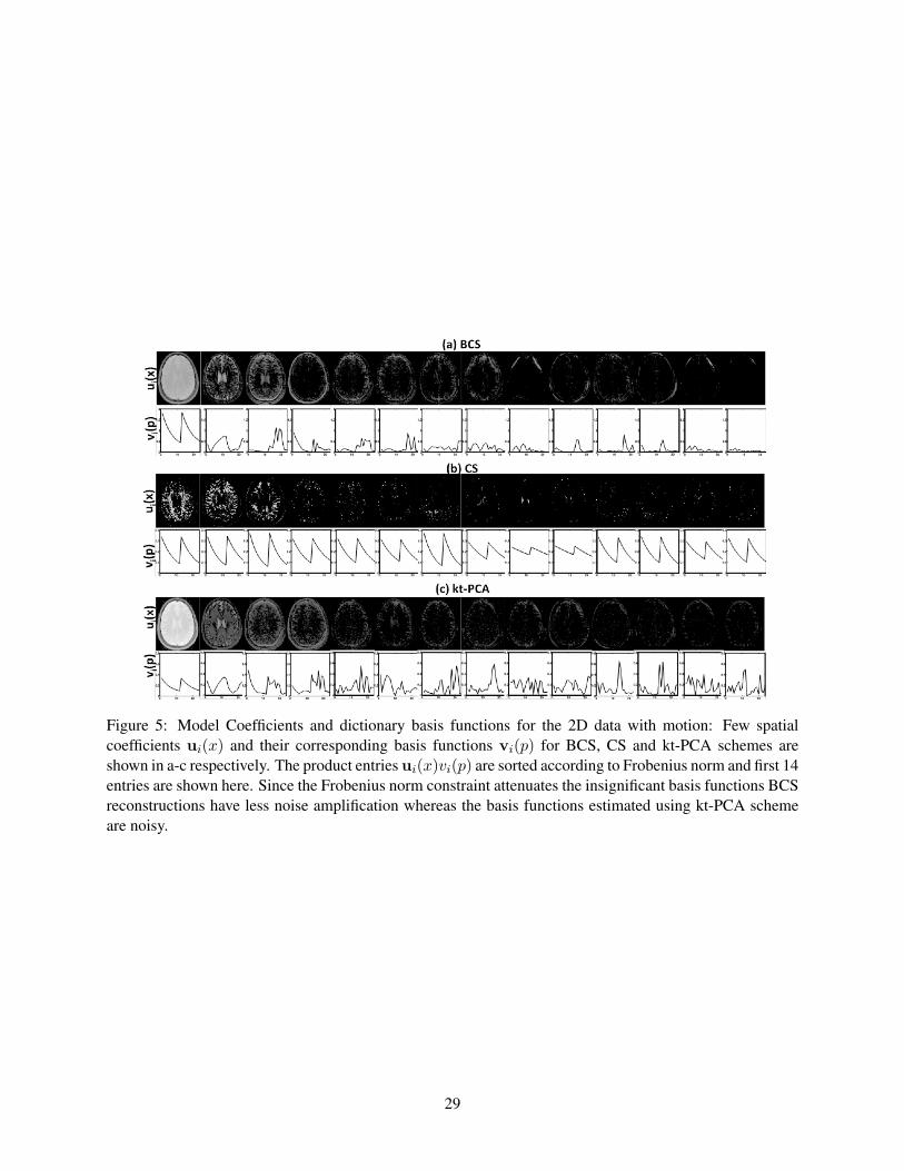
Figure 5: Model Coefficients and dictionary basis functions for the 2D data with motion: Few spatialcoefficients ui(x) and their corresponding basis functions vi(p) for BCS, CS and kt-PCA schemes areshown in a-c respectively. The product entries ui(x)vi(p) are sorted according to Frobenius norm and first 14entries are shown here. Since the Frobenius norm constraint attenuates the insignificant basis functions BCSreconstructions have less noise amplification whereas the basis functions estimated using kt-PCA schemeare noisy.
29
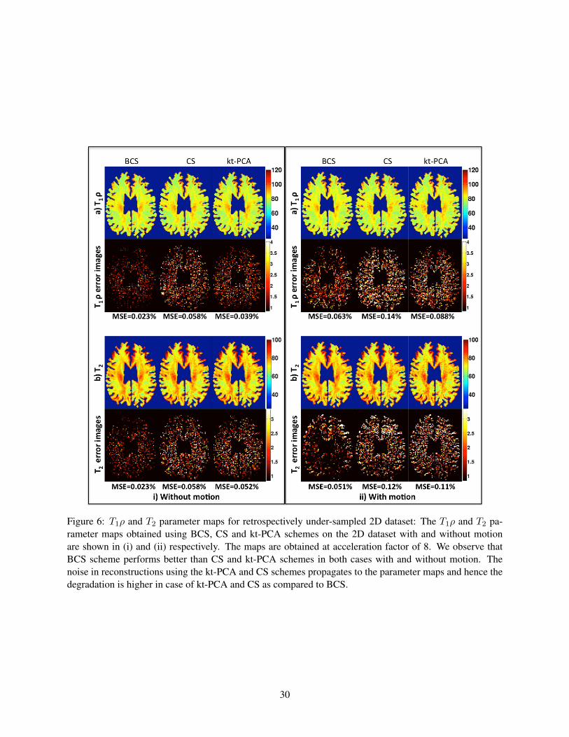
Figure 6: T1ρ and T2 parameter maps for retrospectively under-sampled 2D dataset: The T1ρ and T2 pa-rameter maps obtained using BCS, CS and kt-PCA schemes on the 2D dataset with and without motionare shown in (i) and (ii) respectively. The maps are obtained at acceleration factor of 8. We observe thatBCS scheme performs better than CS and kt-PCA schemes in both cases with and without motion. Thenoise in reconstructions using the kt-PCA and CS schemes propagates to the parameter maps and hence thedegradation is higher in case of kt-PCA and CS as compared to BCS.
30

Figure 7: Parameter maps of a retrospectively under-sampled 2D dataset at different acceleration factors:S0, T1ρ and T2 parameter maps (a-c) at acceleration factors R=1, 6, 8, 10, 12 and, 15 are shown in (i-vi). Weobserve reasonable reconstructions for acceleration factors up to 15 with minimal degradation in contrast.
!"#$%&#'(%)%*' !"#$'(%)%*'
'+,-'.//%/'
0#1234'5+,-'6+78' 93:'5+,-'6+78' 3:'5+,-'6+78'
0#1234'5+,-8' 93:'5+,-8' 3:'5+,-'8'
Figure 8: Comparison of T1ρ maps errors obtained from reconstructions of combined (T1ρ + T2) datasetand the T1ρ only dataset: The T1ρmaps errors at different accelerations for all the schemes on the combineddataset (solid lines) and only T1ρ dataset (dotted lines) are shown. The plot on left shows comparisons forthe datasets without any motion and the plot on the right shows comparisons for datasets with motion. Weobserve in both cases that BCS performs better than CS and kt-PCA schemes. In other words combining thedatasets improves the reconstructions.
31

Figure 9: Choice of regularization parameter λ : The λ parameter was optimized using the L- curve strategy(38). We change λ and plot the data consistency error against the smoothness penalty. λ value of 0.07 waschosen as the regularizing parameter for the 3D dataset.
32

Figure 10: Parameter maps for 3D prospective under-sampled data at R=8: Axial, Coronal and Sagittal T1ρand T2 parameter maps are shown in (i)-(ii). With the acceleration of R=8, the scan time was reduced to 20min. Note: All 128 slices were processed slice by slice to reconstruct the 3D parameter maps
33