Spectral Image Models of Planetary Systemsfor Simulating Exoplanet Observations

Item Type text; Electronic Thesis

Authors Lincowski, Andrew Peter

Publisher The University of Arizona.

Rights Copyright © is held by the author. Digital access to this materialis made possible by the University Libraries, University of Arizona.Further transmission, reproduction or presentation (such aspublic display or performance) of protected items is prohibitedexcept with permission of the author.

Download date 13/06/2018 08:32:04

Link to Item http://hdl.handle.net/10150/579279

– 3 –

ABSTRACT

Future missions to characterize exoplanets will require instruments tailored tofinding a habitable exoplanet: suppressing the bright star while still directly

observing planets at small angular separations. This problem is compounded byinterplanetary dust, a significant source of astrophysical background noise.

Instrument parameters must be constrained with detailed simulations, which canbe analyzed to determine if the instruments are capable of discerning the desired

exoplanet characteristics.A single observation of a planetary disk could constrain the mass of an

exoplanet, an important parameter to identify an exoplanet as terrestrial, if thedust distribution varies by mass sufficiently to be distinguished by future

instruments. As part of the NASA Haystacks team, this thesis presents work incompleting high-fidelity spectral image cubes of our Solar System. New planetary

system architectures are presented, designed to test whether we can distinguishbetween small and intermediate-mass planets by their effects on the dust

structure. These spectral image cubes will be made available for processingthrough instrument simulators for future missions, allowing comparison of known

disk structure with simulated observations of the disk.

– 4 –

1. INTRODUCTION

Exoplanets are an exciting and popular topic in Astronomy. This is also true in the

public’s eye: exoplanets capture the public’s imagination. In addition, the explosion of

new data and discoveries has fueled the field. We know that there are many planets out

there, some with similar properties to those in our Solar System and some very different.

The Kepler mission has discovered thousands of exoplanet candidates. Most systems have

exoplanets and many have more than one (Cassan et al. 2012). Some of these have the

potential to be Earth-like planets. Unfortunately, current telescopes cannot provide the

contrast to directly image an Earth-like planet in the habitable zone. The exact radius

of the habitable zone around a particular planetary system is determined with different

assumptions by different astronomers. Generally, it is the region around a star where we

believe life could exist—for which one metric is where liquid water can exist on the planet’s

surface.

Future telescope missions will seek to find and image an Earth-like planet in the

habitable zone. The consensus is this will require 10−10 suppression of starlight for Sun-like

stars, (Postman et al. 2009). Even the next NASA flagship mission launch, the James

Webb Space Telescope, will not be capable of this. Flagship mission proposals under

development have the goal of imaging exoEarths. One such pending proposal is ATLAST,

the Advanced Technology Large Aperature Space Telescope. An important part of planning

such a mission (that could potentially see first light in the 2030’s) is to define the required

parameters to determine mission success: what are the engineering specifications in order

to find an exoEarth? Under what dust conditions will the future telescope find an exoEarth

and with what yield or probability of success? What specifications are required in order to

show signs of life? Computer simulations can assist in understanding what specifications

are required and help plan observing strategies to maximize the chances of mission success.

Astronomers can use computer programs to simulate telescope instruments. These

programs require input images at specific wavelengths to analyze the impact of diffraction

– 5 –

and other effects of light propagating through an instrument. High-fidelity input images are

required for future telescope missions, which have will high spatial resolution. The results

of model input images processed through an instrument simulator can determine if that

instrument is capable of observing the detail required for astronomers to analyze and find

what is sought: signs of life on an exoplanet and the ability to determine what those signs

are.

Spectroscopy of habitable planets generally require space-based missions because the

same spectral features that are interesting to study in an exoplanet atmosphere are not

readily visible to observers on Earth’s surface, because Earth’s atmosphere has those same

molecules. There are large “dead-zones” in the optical and infrared wavelengths when

observing through Earth’s atmosphere. This research is part of a larger project to develop

the ATLAST mission concept and required observations.

2. A SOLAR SYSTEM MODEL

There is an abundance of information about the structure and composition of our

Solar System. However, we have not observed how the Solar System appears to an outside

observer. This project, nicknamed “Haystacks”, integrates data models and observations

from multiple sources to compile a single, self-consistent model of the Solar System as

seen by an outside observer (Roberge et al. 2015). The model is an integrated spectral

image cube—a three-dimensional data array containing two-dimensional images at a

discrete number of separate wavelengths. Scattered light from the Sun is the primary

source of light for the wavelength range of interest for exoplanet observations (optical to

near-infrared). The primary components resent in observations are dust, the planets, the

star, and the background sources. Other sources, such as the asteroid belt, are insignificant

and unobservable in direct observation.

The Haystacks framework provides an integrated spectral image model of the Solar

– 6 –

System spanning four hundred wavelengths, from 0.3 µm to 2.5 µm. This model can be

viewed at any desired inclination, with or without the Sun’s direct flux, and with or without

the flux of light from local dust.

2.1. Observational Contamination: Dust

The dust is modeled in two different ways, which are catagorized as the inner and outer

Solar System and whose constituent particles are from different sources. The inner Solar

System dust, called zodiacal dust, is primarily from outgassing of Jupiter-sourced comets

(Nesvorny et al. 2010). The inner Solar System is generated in the spectral data cubes using

a custom version of an IDL program called ZODIPIC (Moran et al. 2004). ZODIPIC uses

the Kelsall model (Kelsall et al. 1998) of the local zodiacal dust (from the Diverse Infrared

Background Experiment, DIRBE, onboard the Cosmic Background Explorer, COBE) and

generates spectral images of the inner Solar System (up to 3.28 AU, the location of the 2:1

Jupiter mean motion resonance). The DIRBE experiment provided infrared flux data for

the inner Solar System at ten discrete wavelengths. ZODIPIC uses an analytical fit to this

model to generate scattering flux images (it is also capable of calculating thermal emission)

at any wavelength (Roberge et al. 2015). These are smooth, analytical images, which lack

the Poisson noise present in N-body simulations due to the finite distribution of particles.

The outer Solar System dust originates from particle and small body collisions within

the Kuiper Belt, which has not been directly observed but has been modeled by Kuchner &

Stark (2010). Kuchner & Stark conducted N-body simulations including particle collisions,

resulting in model particle distributions for various particle sizes within 150 AU of the Sun.

Haystacks utilizes the dustmap program (Stark 2011) to compute the scattering of light on

these model dust distributions. The dustmap program generates scattered light flux images,

which were incorporated directly into the Haystacks models. Dustmap calculates the

scattered light flux from the various particle distributions and handles multiple wavelengths.

The scattered light flux images are generated using user-defined parameters, such as the

– 7 –

luminosity of the star, properties of dust particles, and orientation of the disk to the

observer. This program is designed to work for a variety of dust distributions, not just

those for the Solar System. Dustmap is also capable of thermal emission calculation. At the

wavelengths included in the Haystacks model, thermal emission is insignificant compared to

scattered light, and is not included.

The combined dust model must also include the influence of the planets, whose

gravitational effects were included in both the ZODIPIC program and Kuchner & Stark

models. The important dust artifacts in the inner Solar System are the asteroid belts, dust

rings and bands, and blob of dust trailing in Earth’s wake, all revealed from the DIRBE

mission (Kelsall et al. 1998) The ring and blob are shown in Fig. 1. The steady-state

distribution of dust from Kuchner & Stark was generated in the Sun-Neptune co-rotating

frame, which means that all dust features were azimuthally smoothed except for that

co-rotating with Neptune. Thus, outer Solar System includes the area swept out by the

gravitational influence of Jupiter and the smaller area swept out around Neptune.

Fig. 1.— False color image of the inner Solar Sys-tem viewed at 60 degrees from face-on, showing thedust ring and Earth-trailing blob, with the zodicalcloud surpressed.

The other observational contaminant, background sources,(e.g. other stars, galaxies, et

al) are still under development, separately.

– 8 –

2.2. Light Scattering

The scattering of light from small particles is described by the scattering phase function

(SPF), which provides the dependence of light scattering intensity by direction in relation

to the incident wave of light. That is, forward scattering is where the light wave is more

likely to scatter around the dust grain and continue forward, while backscattering is the

reflectance of light off the particle back toward its source.

Dustmap originally utilized the scattering phase function of Hong, a linear combination

of three Henyey-Greenstein scattering phase functions (Hong 1985), which is an empirical

approximation of light scattering from dust grains. Due to unphysical values at extreme

angles, a new version of dustmap was released (v3.1) that utilized Mie Theory to calculate

phase angle for scattered light. Mie Theory is derived from the fundamental principles

of electromagnetism (i.e. it is a solution of Maxwell’s equations). This theory utilizes

an important assumption—spherical particles. Mie Theory results in a SPF that is very

strongly forward-scattering and somewhat back-scattering. This resulted in vastly different

images than those generated using the Hong SPF. These images were not consistent with

general astronomical observations of other debris disks. One possibility is that dust grains

are not well-approximated as spherical (Fig. 2). Therefore, a self-consistent empirical

approximation was used: a single Henyey-Greenstein SPF.

Fig. 2.— Image of a representative dust grain imagedby an electron microscope. Less than one-tenth of amillimeter across, the particle is composed of millionsof even tinier crystals. Interplanetary origin is estab-lished by analyzing the gases that they trapped fromthe Sun while still in space. The interplanetary dustis believed to come from comets, which shed materialas they are warmed by the Sun. Credit: NASA.

– 9 –

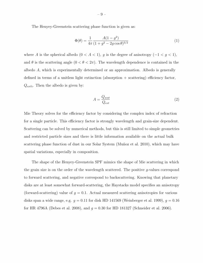
The Henyey-Greenstein scattering phase function is given as:

Φ(θ) =1

4π

A(1− g2)(1 + g2 − 2g cos θ)3/2

(1)

where A is the spherical albedo (0 < A < 1), g is the degree of anisotropy (−1 < g < 1),

and θ is the scattering angle (0 < θ < 2π). The wavelength dependence is contained in the

albedo A, which is experimentally determined or an approximation. Albedo is generally

defined in terms of a unitless light extinction (absorption + scattering) efficiency factor,

Qextλ. Then the albedo is given by:

A =Qscat

Qext

(2)

Mie Theory solves for the efficiency factor by considering the complex index of refraction

for a single particle. This efficiency factor is strongly wavelength and grain-size dependent.

Scattering can be solved by numerical methods, but this is still limited to simple geometries

and restricted particle sizes and there is little information available on the actual bulk

scattering phase function of dust in our Solar System (Munoz et al. 2010), which may have

spatial variations, especially in composition.

The shape of the Henyey-Greenstein SPF mimics the shape of Mie scattering in which

the grain size is on the order of the wavelength scattered. The positive g-values correspond

to forward scattering, and negative correspond to backscattering. Knowing that planetary

disks are at least somewhat forward-scattering, the Haystacks model specifies an anisotropy

(forward-scattering) value of g = 0.1. Actual measured scattering anisotropies for various

disks span a wide range, e.g. g = 0.11 for disk HD 141569 (Weinberger et al. 1999), g = 0.16

for HR 4796A (Debes et al. 2008), and g = 0.30 for HD 181327 (Schneider et al. 2006).

– 10 –

2.3. Model Integration

The problem in constructing a complete model of the Solar System here is to seamlessly

integrate the available models of the inner and outer Solar System. These differing models

are both capable of providing scattered-light-flux images using the appropriate tools

(ZODIPIC for the Kelsall model and dustmap for the Kuchner & Stark models). The

complication for forming a single, self-consistent spectral image cube results from the

fundamentally different natures of these two models and their separate code framework.

The inner Solar System images are smooth and analytic calcations of the scattered light

flux. The Kuiper Belt images result from dynamically-derived three-dimensional dust

distributions, upon which light scattering theory is applied to present an image of scattered

light. Several different methods of interpolation were attempted.

Fig. 3.— False color scattered light im-age of the Solar System in logarithmicscale viewed at 10 parsecs at λ = 900nm. The inner Solar System was gen-erated by ZODIPIC and replaces the in-ner Solar System within an image gener-ated by dustmap. No attempt was madein this combined image to smoothly con-nect the two models, which works ade-quately for a face-on viewpoint. Noticethe abrupt change in brightness from theinner Solar System. It is this area that re-quires estimation because the dust distri-bution of the Solar System in this area isunknown. However, the lower density ofdust in that area can be attributed to thegravitational influence of Jupiter, sweep-ing dust out of its orbit.

The Kuiper Belt dust distribution from Kuchner & Stark was estimated to be only

accurate in to about ∼5 AU or so from the star, to the point where a natural shelf occurs,

and inward of which there is significant Poisson noise (Stark et al. 2015). However this

model still formed an inner dust cloud; interestingly, this was most significant within

– 11 –

about 3 AU, the end of the zodiacal cloud (Grun et al. 1997). Nevertheless, the models

still required merging, the inner portions of the image from the Kuiper Belt had to be

overwritten or combined in some way with the inner Solar System.

Since the inner Solar System model is determined from measurements, the image

generated by ZODIPIC must replace the image generated by dustmap. Although there is

a dust distribution within the entire radii of the dustmap images, the dust distribution

represents Kuiper Belt-sourced dust. Inner Solar System dust is believed to orginate

primarily from Jupiter-sourced comets (Nesvorny et al. 2010). Although the model from

the collisional data files from Kuchner & Stark includes dust that migrated to the center of

the disk, it does not include all sources of dust present in the zodiacal cloud. Therefore,

other methods must be used to bridge the gap between the models.

Therefore, I attempted to use pixel-by-pixel logic to overlay the inner Solar System

image into the disk. The logic was to keep the pixel from whichever model was brighter

for each pixel. This neglects the additive effect of the light scattered through the plane of

the disk for edge-on images. For very forward scattering grains, this can be a strong effect

(Stark et al. 2015). However, at the chosen value of scattering anisotropy (g = 0.1), this

effect is negligble. Furthermore, if one were to attempt to overcome this by simple linear

addition of the images, flux of the inner Solar System will be overstated by effectively

double-counting the effects of dust from the Kuiper Belt in the inner Solar System.

There were several other problems to be addressed, including the aforementioned

region between 3 and 5 AU and the issues with inclined cases. These were handled by

enabling a function in ZODIPIC, which allowed use of a three-dimensional radial power-law

extrapolation from the zodiacal cloud and functions at any disk inclination. (Strubbe &

Chiang 2006) found that the surface brightness of a corpuscular and Poynting-Robertson

(CPR)-dominated disk scales as ∝ r−9/2, the dominant regime inside the primary dust

source (“birth ring”), which in the Solar System is the Kuiper Belt.

As a result, a pixel-by-pixel overlay of the inner Solar System as generated by ZODIPIC

– 12 –

and the Kuiper Belt-sourced dust as imaged by dustmap was used. This is not a perfect

method, but results in smooth and consistent images that can be used for instrument

simulations.

2.4. Image Processing

Although noise is expected from observations, that noise is the result of the instruments

and the discrete nature of incoming photons. Since dustmap generates images from discrete

particle distributions, inevitably the images produced have a degree of Poisson noise. When

observing real astronomical objects, the number of particles emitting or scattering light are

too small to resolve, resulting in a large number of light sources per detector pixel. This is

not the case in a finite-particle simulation such as the dust distributions used to model the

Solar System. This finite particle distribution causes noise that would not be present in

physical viewing. To provide for the ideal source for image simulation, this noise must be

curtailed. If Poisson noise in the images is necessary to simulate photon noise, this should

be applied uniformly to the images, rather than just one component.

Image processing of noise generally involves one of a few smoothing methods. One

simple way is boxcar smoothing, where a pixel is averaged with its immediate neighbors

in a box of defined size. This was the original method attempted in the Haystacks model.

Due to image artifacts resulting from the boxcar smoothing algorithm, Gaussian kernel

smoothing, also called a “Gaussian blur” in image processing, was evaluated. The Gaussian

smoothing was completed using the IDL function GAUSS SMOOTH. The function assumes a

standard deviation of one unless otherwise specified and specifies that the kernel contains

approximately three standard deviations in each direction.

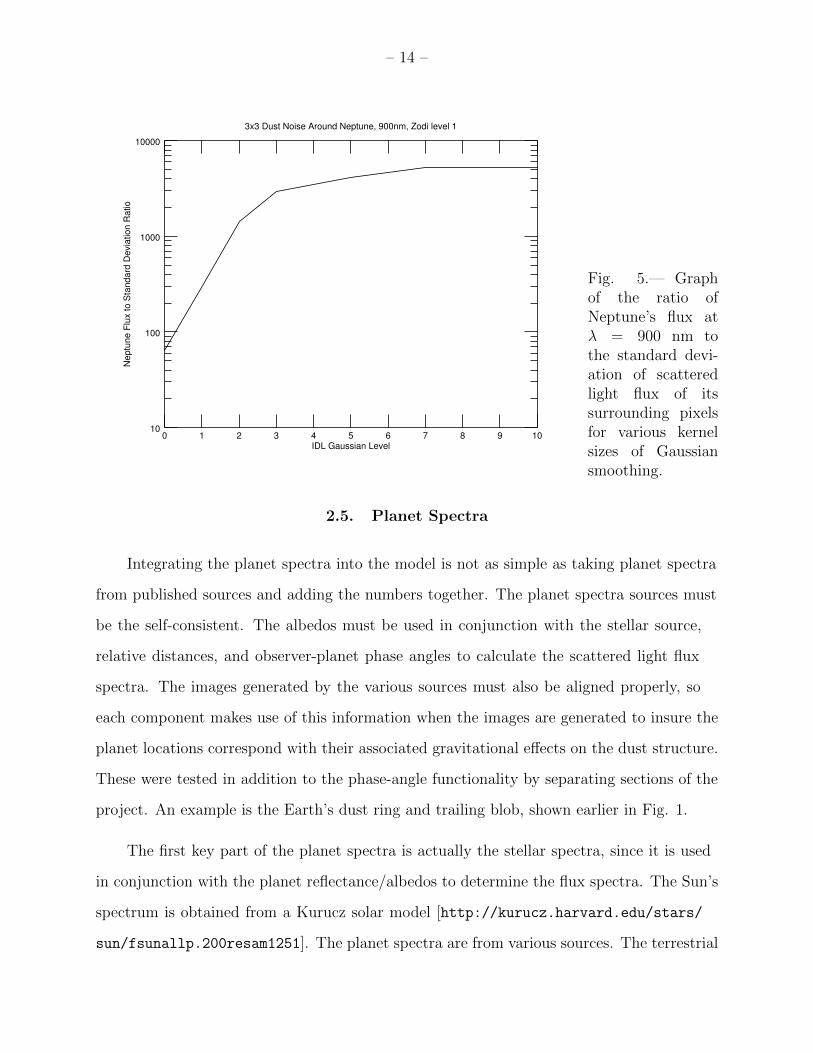
To determine the useful extent of smoothing, images were generated with various kernel

sizes (up to 10) and the smoothing around Neptune’s location was graphed. The planet’s

flux should be at least several times above the standard deviation of the surrounding dust

– 13 –

Fig. 4.— False color scattered light images of the Kuiper Belt-sourced dust in linear scaleviewed at 10 parsecs, λ = 550 nm, viewed face-on. Left image is before smoothing procedure;right image is after Gaussian smoothing using a kernel size of 8.

in order to be detected and distinguishable from the surrounding dust.

As shown in Fig. 5, there was a point of diminishing returns where larger Gaussian

kernel sizes did not result in any improvement in the image. A kernel size of 8 pixels

was chosen to provide for sufficient smoothness. This size was useful for image sizes of

1500x1500 pixels. Smaller images should use a smaller kernel. However, larger images will

not necessarily provide more detail due to the limited number of particles in the Kuiper

Belt model. If larger images are desired, it is more computationally efficient to generate

at the 1500x1500 resolution and enlarge the image. When large-resolution images (e.g.

10000x10000) were generated, there were insufficient particles to support the image size.

When smoothed to a reasonable degree, the image was no different in detail than the

1500x1500 image. For instrument simulator purposes, since the planets and Sun are point

sources, the resize must be executed on the disk portion and should preserve total flux, to

maintain consistent modeling. The dust flux can be enlarged using a command like IDL’s

REBIN. For this command, the image can be enlarged by the desired factor, and then the

pixel values should be divided by the total factor to maintain the same total flux.

– 14 –

3x3 Dust Noise Around Neptune, 900nm, Zodi level 1

0 1 2 3 4 5 6 7 8 9 10IDL Gaussian Level

10

100

1000

10000

Neptu

ne F

lux to S

tan

da

rd D

evia

tion R

atio

Fig. 5.— Graphof the ratio ofNeptune’s flux atλ = 900 nm tothe standard devi-ation of scatteredlight flux of itssurrounding pixelsfor various kernelsizes of Gaussiansmoothing.

2.5. Planet Spectra

Integrating the planet spectra into the model is not as simple as taking planet spectra

from published sources and adding the numbers together. The planet spectra sources must

be the self-consistent. The albedos must be used in conjunction with the stellar source,

relative distances, and observer-planet phase angles to calculate the scattered light flux

spectra. The images generated by the various sources must also be aligned properly, so

each component makes use of this information when the images are generated to insure the

planet locations correspond with their associated gravitational effects on the dust structure.

These were tested in addition to the phase-angle functionality by separating sections of the

project. An example is the Earth’s dust ring and trailing blob, shown earlier in Fig. 1.

The first key part of the planet spectra is actually the stellar spectra, since it is used

in conjunction with the planet reflectance/albedos to determine the flux spectra. The Sun’s

spectrum is obtained from a Kurucz solar model [http://kurucz.harvard.edu/stars/

sun/fsunallp.200resam1251]. The planet spectra are from various sources. The terrestrial

– 15 –

planet spectra are from the Virtual Planet Laboratory’s Spectral Mapping Atmospheric

Radiative Transfer (SMART) models (Meadows & Crisp 1996; Crisp 1997; Robinson 2014).

The model of the Earth was verified by EPOXI observations. The giant planet spectra

are from two observation-based sources: Karkoschka (1998) for 0.3 to 0.9 microns and the

NASA IRTF Spectral Library for 0.9 to 2.5 microns (Rayner et al. 2009). The different

sources of albedo are slightly different and required some adjustment to be consistent (this

work was completd by Dr. Roberge). The Haystacks code uses these normalized geometric

albedos, the solar Kurucz spectrum, and the orbital parameters to determine the actual

scattered light flux for the generated images. In particular, the scattered light flux depends

on distance between the planets and the Sun, their phase angle, and the distance to the

observer. Plotted spectra are shown in Fig. 6.

Solar System Planet Spectra

0.5 1.0 1.5 2.0 2.5

Wavelength (µm)

10−18

10−16

10−14

10−12

10−10

10−8

10−6

Flu

x (

Jy)

VenusEarthMars

Jupiter

SaturnUranus

Neptune

Fig. 6.— Combinedplanet spectra utilized inHaystacks Solar Systemmodel. Haystacks interpo-lates between wavelengthsto construct the spectralimage cube at the desiredwavelenghts between 0.3and 2.5 microns.

2.6. Programming Enhancements

The main Haystacks code runs in the Interactive Data Language (IDL). Computationally

intensive work executed by dustmap utilizes C code, which runs must faster than interpretive

– 16 –

languages. However, it is only written to run sequentially on one processor thread. Modern

computers, even laptops, typically utilize multiple processor cores. Since the four-hundred-

wavelength spectra image cube requires multiple independent executions of code, this lends

itself to multithreading. IDL is capable of calling child processing by launching another

code and then continuing with the main thread. Due to the tiered code wrappers in

this framework, multithreading logic was written into the main Haystacks code that runs

different wavelenghts in parallel. The Haystacks cubes were already separated into four

final files by wavelength due to memory constraints (the total size of the cube is over 4 GB).

Therefore, maximum performance was on a computer with four or more processor cores.

The Haystacks multithreading ran each of the four wavelength bins concurrently, then

utilized logic to wait until all four processes were completed and saved. Other IDL functions

make their own use of multithreading for sufficiently large datasets such as these. Functions

like the noise smoothing were run sequentially because IDL utilized all the processor cores.

Another enhancement was the additional option of constant scattered light flux

from the observer’s location in our own Solar System. The observer on Earth must look

out through the local zodiacal light, out of the Solar System, toward the system under

observation. Haystacks takes the scattered light flux from its own dust spectral image cube

at the Earth’s location to determine the effect at each wavelength. This is only a constant

value for each, but this represents another background source that astronomers face when

analyzing data and is included as an option in the Haystacks code framework to make

inputs as realistic as possible. This option is requested in a prompt when running the code.

From a development standpoint, it is much easier to view the disk in the ideal situation

without the local light, but will provide more realism when included in images that are

passed through instrument simulators and the subsequent data analysis pipeline.

– 17 –

2.7. Solar System Results

The primary initial result of the completed Haystacks framework is the integrated

spectral image model of the Solar System. This model can be viewed at any desired

inclination, with or without the Sun’s direct flux, and with or without the flux of light from

local dust. Specified in the wrappers is the location of Earth and Neptune to reside along

the x-axis. The model is also capable of choosing the orientation of the planets for a certain

point in time (from the reference epoch J2000). This is coded in the IDL wrappers and is

not an option when running the program.

As can be seen in the accompanying images, significant improvements were made to the

Haystacks models, bringing them from roughly developed to become smooth, self-consistent

models, with a complete set of planet spectra and architecture options. Once finalized,

these spectral image cubes will be published on a NASA website for download.

Additional features that have been mentioned were built into the programming code

to allow for a wider variety of images. The date since epoch J2000 can be specified, thereby

changing the locations of the planets (and azimuthal dust structures). This is especially

interesting when considering inclined cases and is important in analyzing the ability to

distinguish between different classes of planets at different phases.

The image output parameters are easily specified in the main program code.

Specifically, the image size and resolution can be specified near the program header.

Haystacks provides the dustmap and ZODIPIC programs with the requisite parameters to

generate the correct images. Since the purpose of these spectral image cubes are for use

with instrument simulators, generating the proper image size and resolution is important

to match the instrument simulator parameters.

– 18 –

Fig. 7.— False color scattered light images of the Kuiper Belt-sourced dust in logarithmicscale to show full depth of features, viewed at 10 parsecs, λ = 550 nm, from face-on. Leftimage is the state of the model with the inner Solar System image from ZODIPIC repacingthe inner 3 AU of the Kuiper Belt model and layers of cutoffs from 3 AU to 10 AU for thevarious Kuiper Belt sources (hot, cold, plutino); right image represents the final results usingthe full features of Haystacks.

3. PROBING AN EFFECT OF SCATTERING ANISOTROPY:

PSEUDO-ZODI EFFECT

I co-authored a paper (Stark, Kuchner, & Lincowski 2015), wherein we investigated the

strong forward-scattering effects for edge-on disks. This section summarizes a portion of

that work, but no part is taken directly from it. My primary contribution was in modifying

the Haystacks code parameters and framework to produce images used for analysis and

presentation in the paper. The images presented in this work are my own.

For observing exoplanets in planetary systems, a primary source of noise is the light

from the host star scattering from interplanetary dust. The degree of anisotropy in the

scattering of light is described by the scattering phase function (SPF). There are several

regimes in use, such as Rayleigh scattering, Mie Theory, Thomson scattering, and Compton

scattering, which all describe light scattering in certain wavelength regimes. The completed

– 19 –

Haystacks models utilized the Henyey-Greenstein SPF, described in section 2. The value

for the anisotropy chosen for the Solar System model was g = 0.1, which indicates a

mild amount of forward-scattering of light. As discussed, however, the bulk scattering

properties of light in the Solar System (or for many other systems) is unknown. Therefore,

it can be informative to probe the effects of forward scattering anisotropy, because this

can particularly affect the disks observed near edge-on. Fig. 8 shows solutions of the

Henyey-Greenstein SPF for various anisotropy values.

Fig. 8.— Henyey-Greenstein scattering phase function. Left figure in polar coordinates,right figure depicting as a function of angle.

The scattering phase function for real dust is difficult to predict, since real dust grains

may not be well-approximated as spheres. On average, however, a distribution of dust

grains may exhibit some average amount of anisotropy. Many properties are inferred

from images of these disks. Like any image, the data is two-dimensional but the object is

three-dimensional. This can lead to interesting effects. Consider dust that is very forward

scattering. Many planetary disks are observed near edge-on, which means light propagating

out from the central star must pass through the extended disk. However, light also scatters

off other parts of the disk, to either side, and this is how we see the entire disk. Mostly this

extended disk is cold dust. Another source of light is neglected from these models: direct

radiation from the dust. Since we are concerned with exoplanet observation and spectral

analysis for evidence of metabolic processes, we are most interested in near-infrared and

– 20 –

visible spectral sources. The cold dust of the outer regions of a planetary disk have little

emission in this wavelength band, so the dominant light source from these grains are the

scattered starlight. The inner dust cloud of a planetary disk, called exozodiacal dust, is

hot from its proximity to the star. These dust grains both scatter and emit radiation in

the near-infrared and optical wavelength bands. It is expected this inner system dust to

be brighter due to scattering more light per unit time but also due to its own radiation.

However, the exozodiacal cloud is much smaller than the entire disk, which in the case of

our Solar System can be 75-100 AU in radius, compared to the ∼3.28 AU radius of the

zodiacal cloud.

When observed edge-on, there is significantly more dust through which light from the

star must scattered. If there is strong forward-scattering, the light scattering forward from

the star through the disk will be favorably scattered forward toward the observer, while

light propagating obliquely will likewise continue away from the observer.

Since habitable planets are expected within the exozodiacal cloud (Absil et al.

2010), a complication that could be induced in exoplanet observations by the strong

forward-scattering of light is the cold disk can exhibit light scattering in excess of that

expected for isotropic light scattering, raising the measured temperature. This is mistaking

the source of flux to be from radiation rather than light scattering. This could impair

observing exoplanets due to an extended cold disk through which observations are made.

Table 1 gives the results of different forward scattering g-values, with results in Janskys

(10−26 W/m2/Hz). For small forward-scattering biases, the hot inner zodiacal cloud is

much brighter than the Kuiper Belt dust. At extreme cases (g & 0.9), the Kuiper Belt

dust is brighter than the brightest case of the inner zodiacal cloud (no forward-scattering

bias). This makes the inner zodiacal cloud appear brighter and hotter than its effective

temperature, thus this has been called “pseudo-zodi”. One concern is that for strongly

forward-scattering disks, the cold dust can make it even more difficult to observe a

potentially habitable exoplanet, since the Earth in this situation (at quadrature) would

– 21 –

Fig. 9.— Scattered light flux images (units of Janskys), logarithmic scale, at λ = 550 nm.The images are 5.12 AU in width (0.01 AU / pixel). The left pair are g = 0.1, the rightare g = 0.9. The first and third images were generated by ZODIPIC, computing basedon the Kelsall model from DIRBE data. The second and fourth images are modeled from adynamically-generated dust model of the Kuiper Belt with 1000-interval azimuthal averaging.

g Zodi (Jy) KB (Jy) KB excess (Jy)0.1 1.25E-11 2.93E-12 -9.61E-120.3 1.19E-11 3.50E-12 -8.35E-120.5 1.04E-11 5.00E-12 -5.39E-120.7 7.54E-12 9.97E-12 2.43E-120.8 5.34E-12 1.82E-11 1.28E-110.9 2.69E-12 4.67E-11 4.41E-11

0.95 1.31E-12 8.89E-11 8.76E-110.98 5.14E-13 1.03E-10 1.03E-10

Table 1: Flux of one pixel at 1 AU from the center of edge-on images generated modelingour Solar System, with a resolution of 0.01 AU per pixel, at λ = 550 nm. Flux is in unitsof Janskys. For g & 0.7, the scattered light flux from the cold dust of the Kuiper Beltoverwhelms the warmer light from the zodiacal dust of the inner Solar System.

appear with a brightness of 4.68× 10−9 Jy at 10 pc. One consideration for mission concepts

is whether the estimates of the number of habitable planet candidates estimated to be

discovered is overly optimistic, if the estimates fail to take into account the potential for

strongly forward-scattering disks.

Another issue encountered was the presence of Poisson noise from the finite particle

distribution, just as in the original development of the Solar System models. The effect is

aggravated due to the interest in a narrower field of view: of the 150-AU diameter disk, the

area of interest is in the habitable zone, which around a Sun-like star is being considered at

the point around 1 AU. This results in such noise that the difference in scattered light flux

– 22 –

between two adjacent pixels is orders of magnitude. Fig. 10 illustrates this issue.

Fig. 10.— Scattered light flux false color images of Solar System disk, edge-on. Width ofimage is 5.12 AU (0.01 AU / pixel). Units are flux in Janskys on a logarithmic scale, at λ =550 nm. On the left are two images with g = 0.1. On the right are g = 0.9. Of each set, theleft is the image at a single azimuthal angle. On the right of each pair is with an averageusing 1000 intervals of azimuthal angle.

In cases of significant (g & 0.7) forward scattering, for a planetary system like the

Solar System the cold dust of the outer debris disk (e.g. the Kuiper Belt), can appear

brighter than the hot dust, even in visible wavelengths. This is being termed “pseudo-zodi”

because it appears as exozodiacal dust corresponding to the inner planetary system, but in

fact results from the forward-scattering of light by the central star as the light propagates

through the cold dust of the debris disk between the star and the observer. The effect

for face-on observing is opposite: the disk can appear dimmer than for isotropic light

scattering, because the light is mostly scattered forward (radially), rather than up toward

the observer. This effect could result in fewer observable exoplanet discoveries from disks

seen closer to edge-on and interfere with spectroscopy of habitable-zone planet atmospheres.

These issues are discussed in depth by Stark et al. (2015).

4. NEW PLANETARY DISK ARCHITECTURES

Astronomical observing by NASA is primarily through space-based telescopes, which

have the advantage of being above the Earth’s atmosphere, which is effectively opaque

in large and important wavelength bands, especially infrared. Furthermore, space-based

instruments, if shielded from the Sun, can operate at a much lower temperature. The

– 23 –

radiation emitted by the instruments themselves interfere with infrared observing. A

primary drawback of space-based telescopes is the difficulty in servicing them or in restoring

consumables, such as coolant and fuel, in addition to the expense of launching them into

space and the cost of exotic materials to reduce the mass of the assemblies. Therefore, the

observing time is at a premium given the cost and lifespan of the instrument, as compared

to ground-based instruments.

An important aspect of determining the mass of an exoplanet is to eliminate classes

of planets that life is not believed to be able to form. Specifically, the elimination of gas

and ice giants in favor of the lower mass rocky planets. A possibility of constraining the

mass of the planet is the planet’s influence on the distribution of dust in the planetary

disk. For example, a gas giant of Jupiter’s mass (317 M⊕) substantially clears its orbital

neighborhood of dust in an entire ring around the star, with the exception of the “Trojan”

asteroids at the stable orbits of the L4 and L5 Lagrange points (Slyusarev & Belskaya

2014). On the other hand, even a planet of Earth’s mass affects the dust distribution near

its orbit, as evidenced by the dust structures measured by DIRBE (Kelsall et al. 1998). A

further complication is in differentiating a terrestrial-mass planet from intermediate mass

planets, which have received many labels, such as mini Neptunes, Super Earths, and gas

dwarfs (conservatively, all have M . 10M⊕). If a single image of the dust structure around

the disk could eliminate exoplanet candidates from consideration as potentially habitable,

valuable telescope time could be spent on better candidates.

To consider these questions, planetary disks different from the Solar System are

considered. Stark & Kuchner (2009) have several dynamically-generated dust distributions.

These include 1, 5, and 17.2 M⊕ (Neptune) planets at 1 and 5 AU. Unlike the Solar System

models described in section 2, the particles within a certain radius (3/8 AU) are removed

from the simulation as being outside the scope of the model’s physics. This region is

artificially missing dust, which must be replaced. I generated dust distributions for this

region. These dust “plugs” were generated by computing the average number density at

– 24 –

the inner edge of the disk over a small, finite radius (say, ∆r = 0.05 AU). I wrote code that

computed this density for each dust particle distribution for each disk architecture (there

is a dust distribution for each grain size, for each architecture). Then, a dust distribution

was generated in spherical coordinates to “plug” the hole in the disk architectures by the

following procedure:

r = rmin + (rmax − rmin)√χu (3)

φ = φmaxχu (4)

θ = θmin + (θmax − θmin)(1/2 + χn/3.65) (5)

where r is the radius, rmin is the minimum radius, the sublimation distance, rmax is the

maximum radius (3/8 AU), φ is the azimuthal angle (0 ≤ φ ≤ 2π), φmax = 2π, θ is the

polar coordinate (0 ≤ φ ≤ π), θmin and θmax are determined by the program, and the χ’s

are the random numbers, either uniformly distributed between 0 and 1 (χu) or a normal

distribution centered at zero with a standard deviation of 1 (χn). The effect of 1/2 is to

effectively shift the center of the distrubtion to the midplane of the disk (π/2) and the

effect of dividing the random number by 3.65 is to narrow the distribution such that three

standard deviations lie within θmax (3σ = 99.7% of data points).

Generating a uniform particle distribution is not as straight forward in spherical

coordinates as it is in Cartesian coordinates. The complication is due to a linear change

in azimuthal and polar angles as a function of radius. The distribution is not uniform if

one multiplies a random number by each coordinate, as it would be if the coordinates were

Cartesian. In spherical coordinates, multiplying the radial coordinate by a uniform random

number baises the distribution because a smaller fraction of the volume is within r/2, since

V ∝ r3, thus 1/8 of the volume contains fully 1/2 of the particles, which is not uniform. To

correct for this, the radial distribution must be a power of 1/2 as correction. In this way,

the higher values of radius are weighted stronger to account for the inward weighting by

uniform distribution of φ and θ.

– 25 –

The polar angle θ required more careful consideration, since this specifies the

“thickness” of the disk. The thickness does not go to zero as radius goes to zero, because

there is a sublimation radius, rsub, where the dust grains sublimate due to extreme

temperature in that region near the star. This is generally taken to be about 1500 K, or

roughly 0.05 AU from a Sun-like star (Vaidya et al. 2009). The difficulty in matching the

dust distribution in this center region to the remainder of the disk is in smoothly matching

the polar angle and number density. The outlined procedure matches the angle of the

disk. The dust distributions of the disk architectures had very uniform polar angles across

large sections of disk. The number density was calculated by determining the average

number density within a narrow range of radius (0.35 to 0.40 AU). The number of particles

was incorporated into the outlined procedure by array computation, where the number of

particles generated was the closest integer for N = nπr2max, where n is the number density.

This distribution provided for a nearly flawless matching of density between the “plug”

and the disk. The scattered light flux images were then generated by the dustmap program.

A selection of these architectures are shown in Fig. 11 and show no evidence of this “plug”.

The edges in the images result from the computed planetary influence.

Fig. 11.— Scattered light flux false color images of disks with a single planet at 1 AU seenface-on with 10-zodis of dust. Width of image is 5 AU (0.01 AU / pixel). Units are flux inJanskys on a logarithmic scale, at λ = 550 nm. The first image is 1 M⊕ (Earth-mass), thesecond is 5 M⊕, the third is 17.2 M⊕ (Neptune-mass). Note the edges seen in these dustdistributions are real edges, not artifacts of the plugged-in particle distribution. The centerplugs are seamless and occur at 3/8 AU.

– 26 –

As the figures show, there are real differences in the dust structures between an Earth,

SuperEarth/miniNeptune, and Neptune-class planet. The real question is whether current

and future instruments can detect these structures and tell the differences. It is encouraging

to see that there are marked differences between the 1 M⊕ and 5 M⊕ disks, which is the

mass scale where differentiation is most strongly desired.

5. Future Work

The spectral image cubes generated by the Haystacks code framework will be used

in conjunction with instrument simulators to evaluate the detectability of potentially

habiltable planets. The cubes will be made public for use by other scientists. NASA/JPL

has already expressed interest in hosting and utilizing these spectral image models.

Special thanks go to Dr. Aki Roberge, research astrophysicist at NASA/Goddard Space

Flight Center, who supervised the majority of this work. The NASA Science Innovation

Fund provided funding for this work. Thanks also are due to the rest of the Haystacks

Team, who provided many components of this work, especially Dr. Christopher Stark.

– 27 –

REFERENCES

Absil, O., Eiroa, C., Augereau, J.-C., et al. 2010, PASP, 430, 293, conference Series

Cassan, A., Kubas, D., Beaulieu, J. P., et al. 2012, Nature, 481, 167

Crisp, D. 1997, Geophys. Res. Lett., 24, 571

Debes, J. H., Weinberger, A. J., & Schneider, G. 2008, ApJ, 673, L191

Grun, E., Staubach, P., Baguhl, M., et al. 1997, Icarus, 129, 270

Hong, S. S. 1985, A&A, 146, 67

Karkoschka, E. 1998, Icarus, 133, 134

Kelsall, T., Weiland, J. L., Franz, B. A., et al. 1998, ApJ, 508, 44

Kuchner, M. J., & Stark, C. C. 2010, AJ, 140, 1007

Meadows, V. S., & Crisp, D. 1996, J. Geophys. Res., 101, 4595

Moran, S. M., Kuchner, M. J., & Holman, M. J. 2004, ApJ, 612, 1163

Munoz, O., Moreno, F., Guirado, D., et al. 2010, J. Quant. Spec. Radiat. Transf., 111, 187

Nesvorny, D., Jenniskens, P., Levison, H. F., et al. 2010, ApJ, 713, 816

Postman, M., Traub, W., Krist, J., et al. 2009, PASP, 430

Rayner, J. T., Cushing, M. C., & Vacca, W. D. 2009, ApJS, 185, 289, http://irtfweb.

ifa.hawaii.edu/~spex/IRTF_Spectral_Library/index_files/Planets.html

Roberge, A., Rizzo, M. J., Nesvold, E. R., et al. 2015, Finding the Needle in the Haystack:

A High-Fidelity Model of the Solar System for Simulating Exoplanet Observations,

in preparation

Robinson, T. 2014, Personal communication

– 28 –

Schneider, G., Silverstone, M. D., Hines, D. C., et al. 2006, ApJ, 650, 414

Slyusarev, I. G., & Belskaya, I. N. 2014, Solar System Research, 48, 139

Stark, C. C. 2011, AJ, 142, 123

Stark, C. C., & Kuchner, M. J. 2009, ApJ, 707, 543

Stark, C. C., Kuchner, M. J., & Lincowski, A. 2015, ApJ, accepted

Strubbe, L. E., & Chiang, E. I. 2006, ApJ, 648, 652

Vaidya, B., Fendt, C., & Beuther, H. 2009, ApJ, 702, 567

Weinberger, A. J., Becklin, E. E., Schneider, G., et al. 1999, ApJ, 525, L53

This manuscript was prepared with the AAS LATEX macros v5.2.