ORIGINAL PAPER

Above- and belowground treebiomass models for three mangrove species in Tanzania:a nonlinear mixed effects modelling approach

Marco Andrew Njana1 & Ole Martin Bollandsås2 & Tron Eid2& Eliakimu Zahabu1

&

Rogers Ernest Malimbwi1

Received: 23 April 2015 /Accepted: 18 September 2015 /Published online: 14 October 2015# INRA and Springer-Verlag France 2015

Abstract& Keymessage Tested on data fromTanzania, both existingspecies-specific and common biomass models developedelsewhere revealed statistically significant large predictionerrors. Species-specific and common above- and below-ground biomass models for three mangrove species weretherefore developed. The species-specific models fitted bet-ter to data than the common models. The former modelsare recommended for accurate estimation of biomassstored in mangrove forests of Tanzania.& Context Mangroves are essential for climate change mitiga-tion through carbon storage and sequestration. Biomassmodels are important tools for quantifying biomass and car-bon stock. While numerous aboveground biomass models

exist, very few studies have focused on belowground biomass,and among these, mangroves of Africa are hardly or notrepresented.& Aims The aims of the study were to develop above- andbelowground biomass models and to evaluate the predictiveaccuracy of existing aboveground biomass models developedfor mangroves in other regions and neighboring countrieswhen applied on data from Tanzania.& Methods Data was collected through destructive sam-pling of 120 trees (aboveground biomass), among these30 trees were sampled for belowground biomass. Thedata originated from four sites along the Tanzaniancoastline covering three dominant species: Avicenniamarina (Forssk.) Vierh, Sonneratia alba J. Smith, andRhizophora mucronata Lam. The biomass models weredeveloped through mixed modelling leading to fixedeffects/common models and random effects/species-specific models.& Results Both the above- and belowground biomass modelsimproved when random effects (species) were considered.Inclusion of total tree height as predictor variable, in additionto diameter at breast height alone, further improved the modelpredictive accuracy. The tests of existing models from otherregions on our data generally showed large and significantprediction errors for aboveground tree biomass.

Handling Editor: Shuqing Zhao

Contribution of co-authors: Njana: Took part in design of research,responsible for data collection and preparation, and for data analysisand manuscript development.O. M. Bollandsås: Supervising the work including providing technicalguidance on data analysis and commenting on the manuscript.T. Eid: Took part in design of the research, supervising the work,commenting, and manuscript development.E. Zahabu: Supervising the work and commenting on the manuscript.R. Malimbwi: Coordinating the design of research project andcommenting on the manuscript.

* Marco Andrew Njanamarconjana2002@yahoo.com

Ole Martin Bollandsåsole.martin.bollandsas@nmbu.no

Tron Eidtron.eid@nmbu.no

Eliakimu Zahabuzahabue@yahoo.com

Annals of Forest Science (2016) 73:353–369DOI 10.1007/s13595-015-0524-3

Rogers Ernest Malimbwiremalimbwi@yahoo.com

1 Department of Forest Mensuration and Management, SokoineUniversity of Agriculture, P.O. Box 3013, Morogoro, Tanzania

2 Department of Ecology and Natural Resources Management,Norwegian University of Life Sciences, Ås, Norway

& Conclusion Inclusion of random effects resulted intoimproved goodness of fit for both above- and below-ground biomass models. Species-specific models there-fore are recommended for accurate biomass estimationof mangrove forests in Tanzania for both managementand ecological applications. For belowground biomass(S. alba) however, the fixed effects/common model isrecommended.

Keywords Avicennia-Sonneratia-Rhizophora . Carbon .

Fixed and random effects

1 Introduction

Mangroves are forests found in the tropical and subtrop-ical coastlines between 30° south and north of equator(FAO 2007). In Africa, there are mangroves both at thewestern and eastern coasts. At the eastern coast ofAfrica, 14 mangrove species are growing naturally, and10 among these are found in Tanzania. Avicenniamarina (Forssk.) Vierh, Sonneratia alba J. Smith, andRhizophora mucronata Lam. are the three most domi-nant mangrove species in Tanzania (MNRT 1991; Luogaet al. 2004; Nshare et al. 2007).

Mangroves provide a range of goods and services ofbiological and economic importance. In addition, man-groves store large amounts of carbon per unit area(Donato et al. 2011; Murray et al. 2011) and are there-fore also important for climate change mitigation(UNEP 2014). Although mangroves in many countriesare legally protected, for example in Tanzania, Kenya,and South Africa (FAO 2007), mangroves suffer fromdeforestation and forest degradation (Wang et al. 2003).

A climate change mitigation strategy under theUnited Nations Framework Convention on ClimateChange (UNFCCC), aiming at Reducing CarbonEmissions from Deforestation and Forest Degradation(REDD+), offers an opportunity for conservation andmanagement of mangroves. Successful implementationof REDD+ relies on the capabilities of participatingcountries to routinely and reliably monitor changes ofcarbon stocks and associated greenhouse gas emissionsthrough establishment of a Monitoring, Reporting andVerification (MRV) system (Hewson et al. 2013). In linewith this, Tanzania has, under the National ForestryResources Monitoring and Assessment (NAFORMA)program, established a national grid of permanent sam-ple plots, which will be monitored for biomass and car-bon over time (URT 2010). For Tanzania to be able toreport carbon stocks at tier 2 or 3 (IPCC 2003), thedevelopment of country-specific biomass models istherefore imperative.

Biomass models, based on allometric theory, relatingeasily measurable tree variables such as diameter atbreast height (dbh) and total tree height (ht) to biomass,are considered to be the most efficient tools for tree levelbiomass prediction (Brown 1997; IPCC 2007; Chaveet al. 2014). The tree variables used as model input areobtained through forest inventories (Husch et al. 2003;URT 2010). Development of biomass models requiresdestructive sampling of trees. Above- and belowgroundfresh weights of the trees are measured in field, andsubsequently, dry weights are determined by using thedry to fresh weight ratio (DF ratio) derived from oven-dried subsamples. Aboveground biomass usually refers tostem, branch, and foliage, while belowground biomassrefers to all live roots down to 2 mm in diameter(IPCC 2006).

Many models for prediction of both above- and be-lowground biomass of mangrove forests have been de-veloped previously. A review by Komiyama et al.(2008) identified 13 species-specific and two common(i.e., multi-species) models for prediction of above-ground biomass of mangroves, while nine species-specific models and one common model were identifiedfor belowground biomass. Additional studies on man-groves that developed models for prediction of biomassnot present in this review also exist (e.g., Kairo et al.2009; Kauffman and Donato 2012; Sitoe et al. 2014).With the exception of the models developed by Kairoet al. (2009) in Kenya and Sitoe et al. (2014) inMozambique, most of the models have been developedfor mangroves in Asia. The relatively few existingmodels for belowground biomass may be associatedwith the labor-intensive nature of sampling belowgroundbiomass for mangrove tree species (Njana et al. 2015).

No biomass models have been developed for man-groves of Tanzania, yet numerous models have beendeveloped based on data from other regions and somefrom neighboring countries in Africa. If these modelsare applied to quantify biomass of mangroves inTanzania, they would be used beyond their spatial va-lidity. Since mangrove trees may respond differently todifferent environmental conditions, this could also resultinto morphological and architectural differences betweentrees originating from different sites. Furthermore, it isalso important that models are used within valid rangesin terms of species and tree size (dbh and ht). Modelscalibrated on data from other regions are more likely toviolate these requirements. For example, the above-ground model by Chave et al. (2005) is based on man-grove data from a limited geographical area (FrenchGuiana and Guadeloupe); thus, the model does not rep-resent mangroves found in Africa and it does not in-clude any dominant species found in Africa. Similarly,

354 M.A. Njana et al.

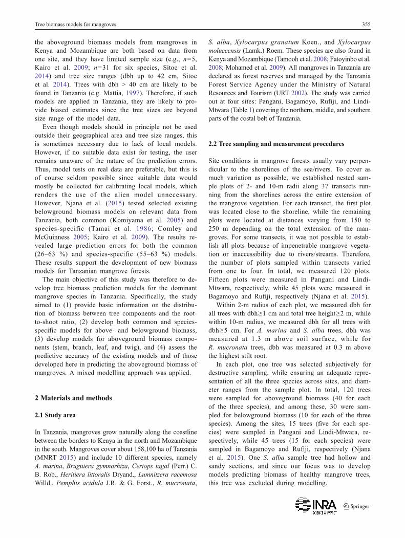
the aboveground biomass models from mangroves inKenya and Mozambique are both based on data fromone site, and they have limited sample size (e.g., n=5,Kairo et al. 2009; n=31 for six species, Sitoe et al.2014) and tree size ranges (dbh up to 42 cm, Sitoeet al. 2014). Trees with dbh > 40 cm are likely to befound in Tanzania (e.g. Mattia, 1997). Therefore, if suchmodels are applied in Tanzania, they are likely to pro-vide biased estimates since the tree sizes are beyondsize range of the model data.

Even though models should in principle not be usedoutside their geographical area and tree size ranges, thisis sometimes necessary due to lack of local models.However, if no suitable data exist for testing, the userremains unaware of the nature of the prediction errors.Thus, model tests on real data are preferable, but this isof course seldom possible since suitable data wouldmostly be collected for calibrating local models, whichrenders the use of the alien model unnecessary.However, Njana et al. (2015) tested selected existingbelowground biomass models on relevant data fromTanzania, both common (Komiyama et al. 2005) andspecies-specific (Tamai et al. 1986; Comley andMcGuinness 2005; Kairo et al. 2009). The results re-vealed large prediction errors for both the common(26–63 %) and species-specific (55–63 %) models.These results support the development of new biomassmodels for Tanzanian mangrove forests.

The main objective of this study was therefore to de-velop tree biomass prediction models for the dominantmangrove species in Tanzania. Specifically, the studyaimed to (1) provide basic information on the distribu-tion of biomass between tree components and the root-to-shoot ratio, (2) develop both common and species-specific models for above- and belowground biomass,(3) develop models for aboveground biomass compo-nents (stem, branch, leaf, and twig), and (4) assess thepredictive accuracy of the existing models and of thosedeveloped here in predicting the aboveground biomass ofmangroves. A mixed modelling approach was applied.

2 Materials and methods

2.1 Study area

In Tanzania, mangroves grow naturally along the coastlinebetween the borders to Kenya in the north and Mozambiquein the south. Mangroves cover about 158,100 ha of Tanzania(MNRT 2015) and include 10 different species, namelyA. marina, Bruguiera gymnorhiza, Ceriops tagal (Perr.) C.B. Rob., Heritiera littoralis Dryand., Lumnitzera racemosaWilld., Pemphis acidula J.R. & G. Forst., R. mucronata,

S. alba, Xylocarpus granatum Koen., and Xylocarpusmoluccensis (Lamk.) Roem. These species are also found inKenya andMozambique (Tamooh et al. 2008; Fatoyinbo et al.2008; Mohamed et al. 2009). All mangroves in Tanzania aredeclared as forest reserves and managed by the TanzaniaForest Service Agency under the Ministry of NaturalResources and Tourism (URT 2002). The study was carriedout at four sites: Pangani, Bagamoyo, Rufiji, and Lindi-Mtwara (Table 1) covering the northern, middle, and southernparts of the costal belt of Tanzania.

2.2 Tree sampling and measurement procedures

Site conditions in mangrove forests usually vary perpen-dicular to the shorelines of the sea/rivers. To cover asmuch variation as possible, we established nested sam-ple plots of 2- and 10-m radii along 37 transects run-ning from the shorelines across the entire extension ofthe mangrove vegetation. For each transect, the first plotwas located close to the shoreline, while the remainingplots were located at distances varying from 150 to250 m depending on the total extension of the man-groves. For some transects, it was not possible to estab-lish all plots because of impenetrable mangrove vegeta-tion or inaccessibility due to rivers/streams. Therefore,the number of plots sampled within transects variedfrom one to four. In total, we measured 120 plots.Fifteen plots were measured in Pangani and Lindi-Mtwara, respectively, while 45 plots were measured inBagamoyo and Rufiji, respectively (Njana et al. 2015).

Within 2-m radius of each plot, we measured dbh forall trees with dbh≥1 cm and total tree height≥2 m, whilewithin 10-m radius, we measured dbh for all trees withdbh≥5 cm. For A. marina and S. alba trees, dbh wasmeasured at 1.3 m above soil surface, while forR. mucronata trees, dbh was measured at 0.3 m abovethe highest stilt root.

In each plot, one tree was selected subjectively fordestructive sampling, while ensuring an adequate repre-sentation of all the three species across sites, and diam-eter ranges from the sample plot. In total, 120 treeswere sampled for aboveground biomass (40 for eachof the three species), and among these, 30 were sam-pled for belowground biomass (10 for each of the threespecies). Among the sites, 15 trees (five for each spe-cies) were sampled in Pangani and Lindi-Mtwara, re-spectively, while 45 trees (15 for each species) weresampled in Bagamoyo and Rufiji, respectively (Njanaet al. 2015). One S. alba sample tree had hollow andsandy sections, and since our focus was to developmodels predicting biomass of healthy mangrove trees,this tree was excluded during modelling.

Tree biomass models for mangroves 355

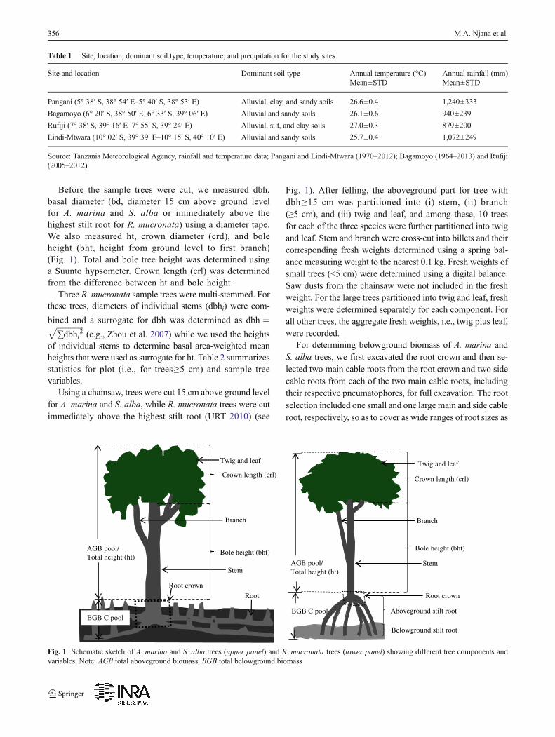
Before the sample trees were cut, we measured dbh,basal diameter (bd, diameter 15 cm above ground levelfor A. marina and S. alba or immediately above thehighest stilt root for R. mucronata) using a diameter tape.We also measured ht, crown diameter (crd), and boleheight (bht, height from ground level to first branch)(Fig. 1). Total and bole tree height was determined usinga Suunto hypsometer. Crown length (crl) was determinedfrom the difference between ht and bole height.

Three R. mucronata sample trees were multi-stemmed. Forthese trees, diameters of individual stems (dbhi) were com-

bined and a surrogate for dbh was determined as dbh ¼ffiffiffiffiffiffiffiffiffiffiffiffiffiffi∑dbhi2

p(e.g., Zhou et al. 2007) while we used the heights

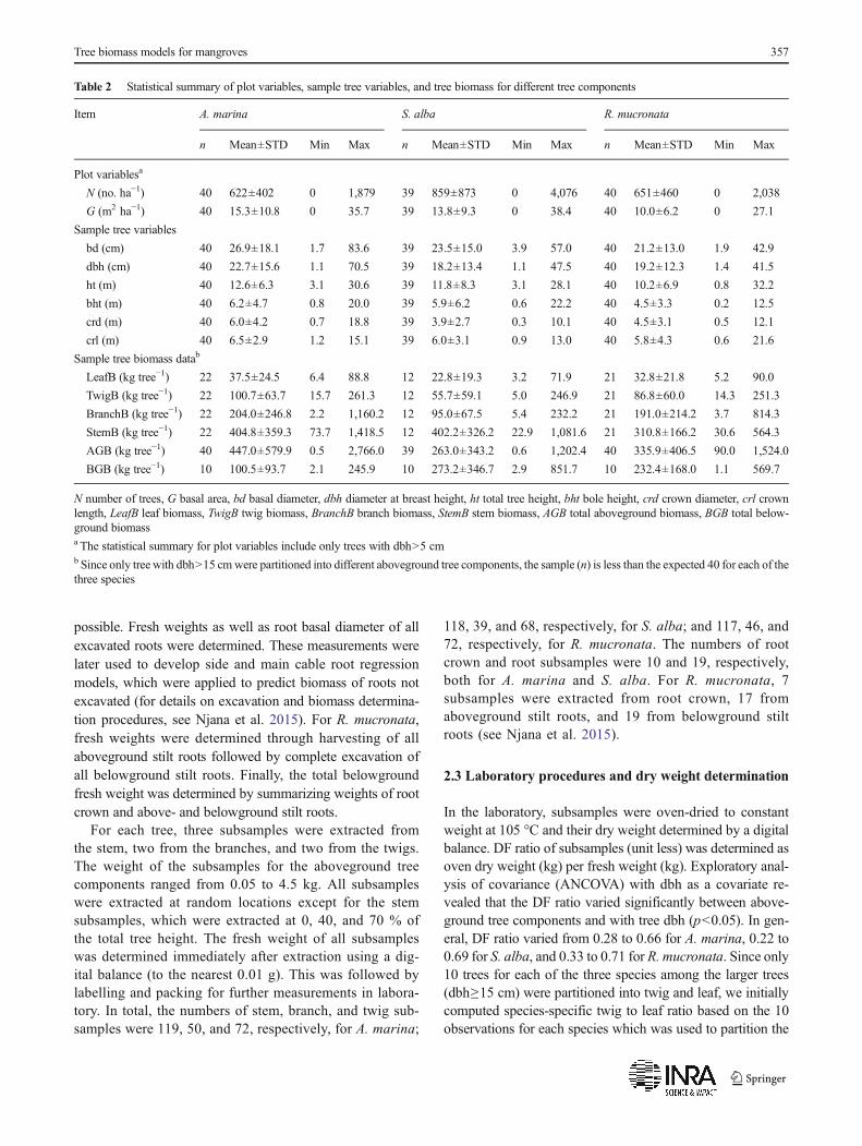
of individual stems to determine basal area-weighted meanheights that were used as surrogate for ht. Table 2 summarizesstatistics for plot (i.e., for trees≥5 cm) and sample treevariables.

Using a chainsaw, trees were cut 15 cm above ground levelfor A. marina and S. alba, while R. mucronata trees were cutimmediately above the highest stilt root (URT 2010) (see

Fig. 1). After felling, the aboveground part for tree withdbh≥15 cm was partitioned into (i) stem, (ii) branch(≥5 cm), and (iii) twig and leaf, and among these, 10 treesfor each of the three species were further partitioned into twigand leaf. Stem and branch were cross-cut into billets and theircorresponding fresh weights determined using a spring bal-ance measuring weight to the nearest 0.1 kg. Fresh weights ofsmall trees (<5 cm) were determined using a digital balance.Saw dusts from the chainsaw were not included in the freshweight. For the large trees partitioned into twig and leaf, freshweights were determined separately for each component. Forall other trees, the aggregate fresh weights, i.e., twig plus leaf,were recorded.

For determining belowground biomass of A. marina andS. alba trees, we first excavated the root crown and then se-lected two main cable roots from the root crown and two sidecable roots from each of the two main cable roots, includingtheir respective pneumatophores, for full excavation. The rootselection included one small and one largemain and side cableroot, respectively, so as to cover as wide ranges of root sizes as

AGB pool/Total height (ht)

BGB C pool

Crown length (crl)

Bole height (bht)

Twig and leaf

Stem

Branch

Root crown

Root

BGB C pool

Crown length (crl)

Bole height (bht)

Twig and leaf

Stem

Branch

Aboveground stilt root

Root crown

AGB pool/Total height (ht)

Belowground stilt root

Fig. 1 Schematic sketch of A. marina and S. alba trees (upper panel) and R. mucronata trees (lower panel) showing different tree components andvariables. Note: AGB total aboveground biomass, BGB total belowground biomass

Table 1 Site, location, dominant soil type, temperature, and precipitation for the study sites

Site and location Dominant soil type Annual temperature (°C) Annual rainfall (mm)Mean±STD Mean±STD

Pangani (5° 38′ S, 38° 54′ E–5° 40′ S, 38° 53′ E) Alluvial, clay, and sandy soils 26.6±0.4 1,240±333

Bagamoyo (6° 20′ S, 38° 50′ E–6° 33′ S, 39° 06′ E) Alluvial and sandy soils 26.1±0.6 940±239

Rufiji (7° 38′ S, 39° 16′ E–7° 55′ S, 39° 24′ E) Alluvial, silt, and clay soils 27.0±0.3 879±200

Lindi-Mtwara (10° 02′ S, 39° 39′ E–10° 15′ S, 40° 10′ E) Alluvial and sandy soils 25.7±0.4 1,072±249

Source: Tanzania Meteorological Agency, rainfall and temperature data; Pangani and Lindi-Mtwara (1970–2012); Bagamoyo (1964–2013) and Rufiji(2005–2012)

356 M.A. Njana et al.

possible. Fresh weights as well as root basal diameter of allexcavated roots were determined. These measurements werelater used to develop side and main cable root regressionmodels, which were applied to predict biomass of roots notexcavated (for details on excavation and biomass determina-tion procedures, see Njana et al. 2015). For R. mucronata,fresh weights were determined through harvesting of allaboveground stilt roots followed by complete excavation ofall belowground stilt roots. Finally, the total belowgroundfresh weight was determined by summarizing weights of rootcrown and above- and belowground stilt roots.

For each tree, three subsamples were extracted fromthe stem, two from the branches, and two from the twigs.The weight of the subsamples for the aboveground treecomponents ranged from 0.05 to 4.5 kg. All subsampleswere extracted at random locations except for the stemsubsamples, which were extracted at 0, 40, and 70 % ofthe total tree height. The fresh weight of all subsampleswas determined immediately after extraction using a dig-ital balance (to the nearest 0.01 g). This was followed bylabelling and packing for further measurements in labora-tory. In total, the numbers of stem, branch, and twig sub-samples were 119, 50, and 72, respectively, for A. marina;

118, 39, and 68, respectively, for S. alba; and 117, 46, and72, respectively, for R. mucronata. The numbers of rootcrown and root subsamples were 10 and 19, respectively,both for A. marina and S. alba. For R. mucronata, 7subsamples were extracted from root crown, 17 fromaboveground stilt roots, and 19 from belowground stiltroots (see Njana et al. 2015).

2.3 Laboratory procedures and dry weight determination

In the laboratory, subsamples were oven-dried to constantweight at 105 °C and their dry weight determined by a digitalbalance. DF ratio of subsamples (unit less) was determined asoven dry weight (kg) per fresh weight (kg). Exploratory anal-ysis of covariance (ANCOVA) with dbh as a covariate re-vealed that the DF ratio varied significantly between above-ground tree components and with tree dbh (p<0.05). In gen-eral, DF ratio varied from 0.28 to 0.66 for A. marina, 0.22 to0.69 for S. alba, and 0.33 to 0.71 for R. mucronata. Since only10 trees for each of the three species among the larger trees(dbh≥15 cm) were partitioned into twig and leaf, we initiallycomputed species-specific twig to leaf ratio based on the 10observations for each species which was used to partition the

Table 2 Statistical summary of plot variables, sample tree variables, and tree biomass for different tree components

Item A. marina S. alba R. mucronata

n Mean±STD Min Max n Mean±STD Min Max n Mean±STD Min Max

Plot variablesa

N (no. ha−1) 40 622±402 0 1,879 39 859±873 0 4,076 40 651±460 0 2,038

G (m2 ha−1) 40 15.3±10.8 0 35.7 39 13.8±9.3 0 38.4 40 10.0±6.2 0 27.1

Sample tree variables

bd (cm) 40 26.9±18.1 1.7 83.6 39 23.5±15.0 3.9 57.0 40 21.2±13.0 1.9 42.9

dbh (cm) 40 22.7±15.6 1.1 70.5 39 18.2±13.4 1.1 47.5 40 19.2±12.3 1.4 41.5

ht (m) 40 12.6±6.3 3.1 30.6 39 11.8±8.3 3.1 28.1 40 10.2±6.9 0.8 32.2

bht (m) 40 6.2±4.7 0.8 20.0 39 5.9±6.2 0.6 22.2 40 4.5±3.3 0.2 12.5

crd (m) 40 6.0±4.2 0.7 18.8 39 3.9±2.7 0.3 10.1 40 4.5±3.1 0.5 12.1

crl (m) 40 6.5±2.9 1.2 15.1 39 6.0±3.1 0.9 13.0 40 5.8±4.3 0.6 21.6

Sample tree biomass datab

LeafB (kg tree−1) 22 37.5±24.5 6.4 88.8 12 22.8±19.3 3.2 71.9 21 32.8±21.8 5.2 90.0

TwigB (kg tree−1) 22 100.7±63.7 15.7 261.3 12 55.7±59.1 5.0 246.9 21 86.8±60.0 14.3 251.3

BranchB (kg tree−1) 22 204.0±246.8 2.2 1,160.2 12 95.0±67.5 5.4 232.2 21 191.0±214.2 3.7 814.3

StemB (kg tree−1) 22 404.8±359.3 73.7 1,418.5 12 402.2±326.2 22.9 1,081.6 21 310.8±166.2 30.6 564.3

AGB (kg tree−1) 40 447.0±579.9 0.5 2,766.0 39 263.0±343.2 0.6 1,202.4 40 335.9±406.5 90.0 1,524.0

BGB (kg tree−1) 10 100.5±93.7 2.1 245.9 10 273.2±346.7 2.9 851.7 10 232.4±168.0 1.1 569.7

N number of trees, G basal area, bd basal diameter, dbh diameter at breast height, ht total tree height, bht bole height, crd crown diameter, crl crownlength, LeafB leaf biomass, TwigB twig biomass, BranchB branch biomass, StemB stem biomass, AGB total aboveground biomass, BGB total below-ground biomassa The statistical summary for plot variables include only trees with dbh>5 cmb Since only tree with dbh>15 cmwere partitioned into different aboveground tree components, the sample (n) is less than the expected 40 for each of thethree species

Tree biomass models for mangroves 357

aggregate twig and leaf component into twig and leaf for treesnot partitioned into that level. Then, total tree abovegroundbiomass was calculated as the product of tree- and component-specific fresh weight and DF ratio:

AGBh ¼Xis¼1

ns

FWhis � DFhsð Þ þXib¼1

nb

FWhib � DFhbð Þ

þXit¼1

nt

FWhit � DFhtð Þ þXil¼1

nl

FWhil � DFhlð Þ

where AGBh = observed total tree aboveground dry weight(kg) of the hth tree, n = total number of billets/twig bundles/leaf weights for a given aboveground tree component, s =stem, b = branch, t = twig, l = leaf, i = ith subsection, FWhis ,FWhib , FWhit , and FWhil are stem, branch, twig, and leaf freshweights (kg), respectively, and DFhs , DFhb , DFht , and DFhlare stem, branch, twig, and leaf DF ratios, respectively.

Belowground dry weight determination for A. marina andS. alba involved conversion of fresh weight of excavated rootcomponents using species-, tree-, and component-specific DFratios. From excavated sample root dry weight data, regres-sion models for prediction of dry weight of unexcavatedroots were developed and dry weights of unexcavatedroots were predicted (for details, see Njana et al. 2015).Therefore, total root dry weights comprised excavatedand unexcavated (i.e., predicted) root dry weights.Total tree belowground dry weight, i.e., belowgroundbiomass, was derived as the sum of root and root crowndry weight. For R. mucronata, tree belowground dryweight was obtained by converting total tree freshweight to dry weight using tree-specific DF ratios.This was the case because for this species, tree below-ground fresh weight was not distinguished into rootcomponents. Statistical summary for sample tree dryweights are presented in Table 2.

2.4 Model specification

Model specification involves selection of functionalform as well as selection of predictor variables.Initially, we tested various functional forms; however,power functional form was the best. Power functionshave been widely used to model biomass of mangrovetrees (e.g., Tamai et al. 1986; Komiyama et al. 2005;Kairo et al. 2009; Ray et al. 2011; Patil et al. 2014). Inthis study, two variants of power functions with anadditive error term (ɛi) were considered (model formsModel form 1 and Model form 2):

Bi ¼ β0 � dbhið Þβ1 þ εi ðModelform1Þ

Bi ¼ β0 � dbhið Þβ1 htið Þβ2 þ εi ðModelform2Þwhere i represent ith observation, and Bi representaboveground biomass, leaf biomass, twig biomass,branch biomass, or stem biomass. Model form Modelform 1 represents biomass as a function of dbhi, whilemodel form Model form 2 represents biomass as a func-tion of both dbhi and hti, while the betas (β) are modelparameters.

Diameter at breast height (dbhi) is highly correlatedwith biomass (Bi). However, also hti is highly correlatedwith biomass and could be a useful variable in biomassmodels to reflect that trees reach their maximum height atan earlier stage than maximum diameter. This means thatmodels depending on dbh only may overpredict biomassof large trees because the biomass increase per unit in-crease in diameter is reduced when trees approach maxi-mum height. Thus, hti represents additional informationnot reflected by dbhi (e.g., Chave et al. 2005).

2.5 Nonlinear mixed effects (NLME) modelling

2.5.1 Nonlinear mixed effects models

Three important assumptions for regression modelling arenormality, homoscedasticity (if residual variance increases asa function of dbh), and independency of residuals. Results andconclusions based on regression analysis are only reliable ifthese assumptions are met (Ritz and Streibig 2008; Zuur et al.2009). For biological data, however, such assumptions may bedifficult to meet. Non-normal residuals, for example, may bedue to outliers, while lack of independency of residuals mayoccur due to the structure of data itself (Zuur et al. 2009). Non-normal and heteroscedastic residuals may be dealt with bytransformation (Ritz and Streibig 2008; Zuur et al. 2009),although this leads into change of the original scale and intro-duces bias (O’Hara and Kotze 2010; Packard 2009).

NLME modelling is one way to confront challenges en-countered in conventional regression approaches since it re-laxes regression assumptions and take into account the com-plex nature of biological data (Pinheiro and Bates 2000; Zuuret al. 2009). Within the mixed effects model framework, pa-rameters may also be allowed to vary by grouping variables(s)(i.e., random variables(s)) (Ritz and Streibig 2008). NLMEmodels may generally be expressed as follows (Lindstromand Bates 1990; Vonesh and Chinchilli 1997; Pinheiro andBates 1998):

yi j ¼ f xi j;λ j;β;α j

� �þ εi j

where i = ith observation, j = jth random-effect variable, yij =response variable for observation i and random-effect variablej, xij = predictor variable for observation i and random-effect

358 M.A. Njana et al.

variable j, λj = random-effect variable for j, β = fixed effectsparameters, αj = random effects parameters, and ɛij = errorterm, which is assumed normally distributed with a mean ofzero.

Our data originated from four different sites and comprisedthree different species, where one tree was destructively sam-pled from each sample plot spatially distributed along tran-sects. Since our data structure is hierarchical and the biomass–dbh relationship is nonlinear (Fig. 2), tree biomass wasmodelled using the NLME modelling approach in order topreserve the original scale.

Biomass models based on mixed effects modellingframeworks have also previously been developed (e.g.,Moore 2010; Li et al. 2011; Xu et al. 2014). The mixedeffects modelling provides a statistical capability wherefixed- (i.e., populations average) and random effects(i.e., group specific) parameters may be estimated simul-taneously (West et al. 2007). Under the mixed effectsmodelling framework, models including fixed effects pa-rameters may therefore be regarded as common ormulti-species models, while those including random ef-fects may be regarded as species-specific models.

2.5.2 Modelling procedures

Model development was carried out using the R software ver-sion 3.1.2 (R Core Team 2014) using the NLME function in

the NLME package (Pinheiro et al. 2015). In order to specifywhich parameter to be treated as solely fixed effects and whichone as both fixed and random effects, we initially tested eachparameter as both fixed and random effects parameters againstprospective random effects variables. Prospective random ef-fects variables included species (j) and site (k). The influenceof random effects variable(s), individually or in combinationon a given parameter, was evaluated using Akaike informationcriteria (AIC). Accordingly, β0 (model forms 1 and 2) and β2(model form 2) were considered as solely a fixed effects pa-rameter, while β1 was considered as both fixed and randomeffects parameters. Model forms 1 and 2 were then re-specified to include a random effects parameter (αjk) (modelforms Model form 3 and Model form 4):

Bi jk ¼ β0 � dbhi jk� �β1þα jk þ εi jk ðModelform3Þ

Bi jk ¼ β0 � dbhi jk� �β1þα jk hti jk

� �β2 þ εi jk ðModelform4Þ

Site did not result into significant random parameters(β1), so relevant parameters estimated were not reported.Three sets of biomass models were developed: (i) above-ground biomass models, (ii) belowground biomassmodels, and (iii) aboveground tree component (leaf, twig,branch, and stem) biomass models. Both model forms 3and 4 were fitted for total aboveground biomass, whileonly model form 3 was fitted for belowground biomassand aboveground tree component biomass. Model form 4was not considered for belowground and abovegroundtree components due to limited number of observations(Harrell 2001; Roxburgh et al. 2015).

During explorative data analysis, we observed that residualvariances (σ2 (ɛijk)) were heteroscedastic. Consequently, we as-sumed heteroscedasticity, and residual variances were modelledas a function of dbh using varPower function in R (Pinheiro andBates 2000; Ritz and Streibig 2008; Zuur et al. 2009);

σ2 εi jk� � ¼ σ2 � dbhi jk

�� ��2ϕwhere ϕ = variance function coefficient. We initially also testedother functions in R (varExp, varIdent, varConstPower, andvarComb). However, the varPower function appeared to bethe best.

The effects of the variance function were evaluatedusing AIC. The variance function is implicitly part ofthe mixed effects model but is not explicitly stated; there-fore, the variance functions are not reported in the results(Smith et al. 2014; de Miguel et al. 2014). Since one treewas sampled from each plot and the distance betweenplots ranged from 150 to 250 m, observations betweenplots were considered spatially independent; thus, no cor-relation structure was assumed.

During tests for random and variance function ef-fects, model parameterization was done by using

0 20 40 60

050

015

0025

00

AGB across species

0 20 40 60

050

015

0025

00

AGB across sites

0 10 20 30 40

020

040

060

080

0

BGB across species

0 10 20 30 40

020

060

010

00

BGB across sites

dbh (cm)

Tre

e bi

omas

s (k

g)

Fig. 2 Above- and belowground tree biomass over dbh across speciesand sites. Symbols black up-pointing triangle, gray up-pointing triangle,and white up-pointing triangle, respectively, represent A. marina, S. alba,and R. mucronata tree species, while black circle, white circle, gray plussign, and black plus sign, respectively, represent trees from Pangani,Bagamoyo, Rufiji, and Lindi-Mtwara. Note: AGB = total abovegroundbiomass, BGB = total belowground biomass

Tree biomass models for mangroves 359

maximum likelihood (ML), while we for the finalmodels used restricted ML (REML) (Lindstrom andBates 1990; Pinheiro and Bates 2000). The models wereevaluated using root mean squared error (RMSE (%))and mean prediction error (MPE (%)) (Chai andDraxler 2014; Walther and Moore 2005) as measuresof goodness of fit while model selection was done usingAIC:

RMSE %ð Þ ¼

ffiffiffiffiffiffiffiffiffiffiffiffiffiffiffiffiffiffiffiffiffiffiffiffiffiffiffiXei jk

2� �.

n

r

MBobs

0BB@

1CCA� 100

MPE %ð Þ ¼X

ei jk� �.

n

MBobs

0@

1A� 100

AIC ¼ n� ln

Xei jk

2� �n

0@

1A

0@

1Aþ 2� pþ 1ð Þ þ C

where eijk = residuals, i.e., difference between predicted andobserved tree biomass (kg), n = sample size, MBobs = meanobserved tree biomass (kg), ln = natural logarithm, p = numberof parameters, and C = constant.

RMSE (%) represents a measure of accuracy and MPE (%)a measure of bias. A model with lower RMSE (%) than thereference model implied the model to be more accurate thanthe referencemodel and vice versa. Similarly, MPE (%) valuessignificantly different from zero implied biased abovegroundbiomass predictions, i.e., under- or overpredictions; otherwise,they implied unbiased aboveground biomass predictions. Thecommonly used model selection criterion R2 was not consid-ered since its use has been criticized (e.g., Johnson andOmland 2004; Sileshi 2014).

2.6 Evaluation of predictive accuracy of existing biomassmodels

Based on a literature review, relevant existing above-ground biomass models were selected and tested onour data to determine their predictive accuracy. The se-lected models ensured representation of various regionsand included four common and eight species-specificbiomass models (Table 3). RMSE (%), MPE (%), andAIC served as model evaluation criteria. After compu-tation of these criteria, the existing models were rankedin descending order based on AIC. The existing modelswere ranked without stratification into model type orpredictor variable included since AIC as a model selec-tion criteria is capable of detecting such differences(Burnham et al. 2011).

3 Results

3.1 Distribution of biomass into different tree parts

The three mangrove species considered in this study storedbetween 49 % (R. mucronata) and 72 % (S. alba) of above-ground biomass in the stem, while the rest in descending orderwas stored in branch, twig, and leaf (Fig. 3). On average,about 41 % of the total tree biomass is stored in the rootsystem (Fig. 4). Figures 3 and 4 show that S. alba had rela-tively higher stem biomass and higher root biomass comparedto the other species. The root-to-shoot ratios for A. marina,S. alba, and R. mucronata were 0.38, 1.29, and 0.62, respec-tively, with an overall mean of 0.70. Generally, the root-to-shoot ratio depicted a decreasing trend from lower to higherdbh classes.

3.2 Biomass models

All parameter estimates for the above- and belowground bio-mass models were statistically significant (Table 4). For theaboveground biomass fixed effects models (FE1, FE2), inclu-sion of ht as a predictor variable was important since RMSEdecreased from 42.6 to 38.4 %, which is equivalent to a de-cline of about 10 %. Based on AIC as model selection criteri-on, the fixed effects model FE2 is better than model FE1. Forthe aboveground biomass random effects models, inclusion ofht resulted in lower RMSE (%) and MPE (%) values forA. marina (models RE1 and RE4) and S. alba (models RE2and RE5), while mixed results were observed forR. mucronata (models RE3 and RE6).

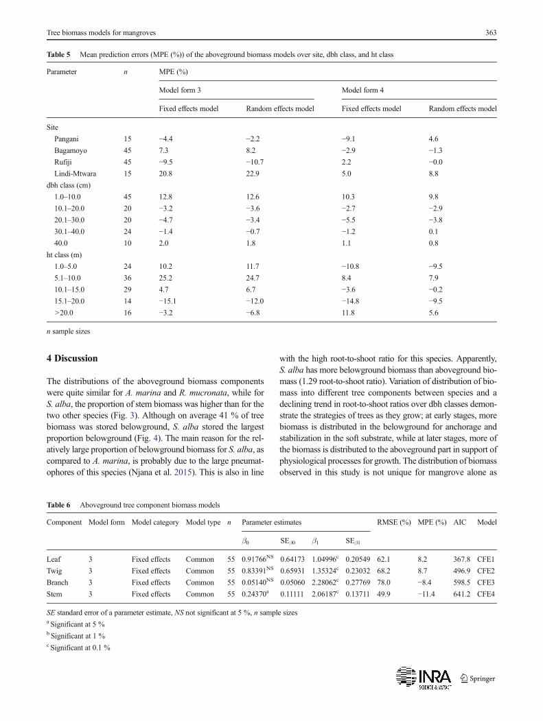
The evaluation of the aboveground biomass models(Table 5) showed that inclusion of ht as predictor variable(model form 4) generally improved predictive accuracy, i.e.,provided lower MPE values. The results also showed that therandom effects models with ht as a predictor variable weremore accurate than the fixed effects models.

For the belowground biomass models (Table 4), the good-ness of fit statistics, i.e., RMSE (%) and MPE (%), improvedwhen using random effects for A. marina (model RE7) andR. mucronata (model RE9) compared to the fixed effectsmodel (model FE3), while the opposite was observed forS. alba (model RE8).

The β0 parameter estimates of the aboveground tree com-ponents biomass models were statistically non-significant(p>0.05) except for the stem biomass model (Table 6). Allother parameter estimates were statistically significant(p<0.05). MPEs were slightly lower than 10 % for the leaf,twig, and branch biomass models, while MPE was slightlyhigher than 10% for the stemmodel. The stem biomass modelhad lower RMSE (%) values compared to all the other com-ponent models.

360 M.A. Njana et al.

Using paired t test, comparisons of observed totaltree aboveground biomass with total tree abovegroundbiomass predicted the tree components common/fixedeffects models showed that the prediction errors were

non-significant for A. marina (n=23, MPE=−6.5 %,p>0.05) and S. alba (n=17, MPE=3.9 %, p>0.05),while they were significant for R. mucronata (n=21,MPE=16.0 %, p<0.05).

Am Sa Rm Overall

LeafTwigBranchStem

020

4060

8010

0

Cum

mul

ativ

e pe

rcen

tage

Fig. 3 Distribution of biomass between aboveground tree components.Am = A. marina (n=23), Sa = S. alba (n=17), and Rm = R. mucronata(n=21)

Am Sa Rm Overall

AGBBGB

020

4060

8010

0

Cum

mul

ativ

e pe

rcen

tage

Fig. 4 Distribution between above- and belowground biomass. Am =A. marina (n=10), Sa = S. alba (n=10), and Rm = R. mucronata (n=10). Note: AGB = total aboveground biomass, BGB = total belowgroundbiomass

Table 3 Existing aboveground biomass mangrove models selected for evaluation of prediction accuracy

Model type Model n R2 RMSE dbh (cm) Location Author

Common AGB=3.254×exp(0.065×dbh) 31 0.89 4.244 0.5–42 Sofala bay,Mozambique

Sitoe et al. (2014)

Common AGB=1.3799×dbh0.955×ht0.687 100 0.98 – – India Ray et al. (2011)

Common AGB=0.0509×ρ(dbh2×ht) 84 0.96 – dbhmax=42 French Guiana andGuadeloupe

Chave et al. (2005)

Common AGB=0.251×ρ×dbh2.46 104 0.98 0.085 5.0–48.9 Thailand and Indonesia Komiyama et al. (2005)

A. marina

Species-specific

AGB=0.3404×dbh2.0273 110 0.94 – – Mumbai, India Patil et al. (2014)

Species-specific

AGB=exp(0.2540+0.9140×log(dbh)) 10 0.31 1.340 8a Gazi Bay, Kenya Kairo et al. (2009)

Species-specific

AGB=0.1036×dbh2+0.5402×dbh+(−1.5674) – 0.94 – 2.1–12.1 Taiwan Kuei (2008)

Species-specific

AGB=0.308×dbh2.11 22 0.97 0.023 dbhmax=35 Darwin, Australia Comley andMcGuinness(2005)

S. alba

Species-specific

AGB=0.0825×ρ×(dbh2×ht)0.89966 345 0.95 – dbhmax=323 Palau Kauffman and Donato(2012)

Species-specific

AGB=exp(0.6715+0.1473×log(dbh)) 10 0.01 0.580 10a Gazi Bay, Kenya Kairo et al. (2009)

R. mucronata

Species-specific

AGB=0.0311×ρ×(dbh2×ht)1.00741 73 0.95 – dbhmax=39.5 Palau Kauffman and Donato(2012)

Species-specific

AGB=exp(−0.1811+0.6590×log(dbh)) 5 0.83 1.050 5a Gazi Bay, Kenya Kairo et al. (2009)

Units of measurement: total aboveground biomass, kilogram; diameter at breast height, centimeter; total height (ht), meter; basic density, gram per cubiccentimeter

AGB total aboveground biomass, dbh diameter at breast height, ht total height, ρ basic density, n sample sizesa The figure refer to the fixed age of planted mangrove trees which is surrogate to dbh

Tree biomass models for mangroves 361

3.3 Evaluation of predictive accuracy of existingaboveground biomass models

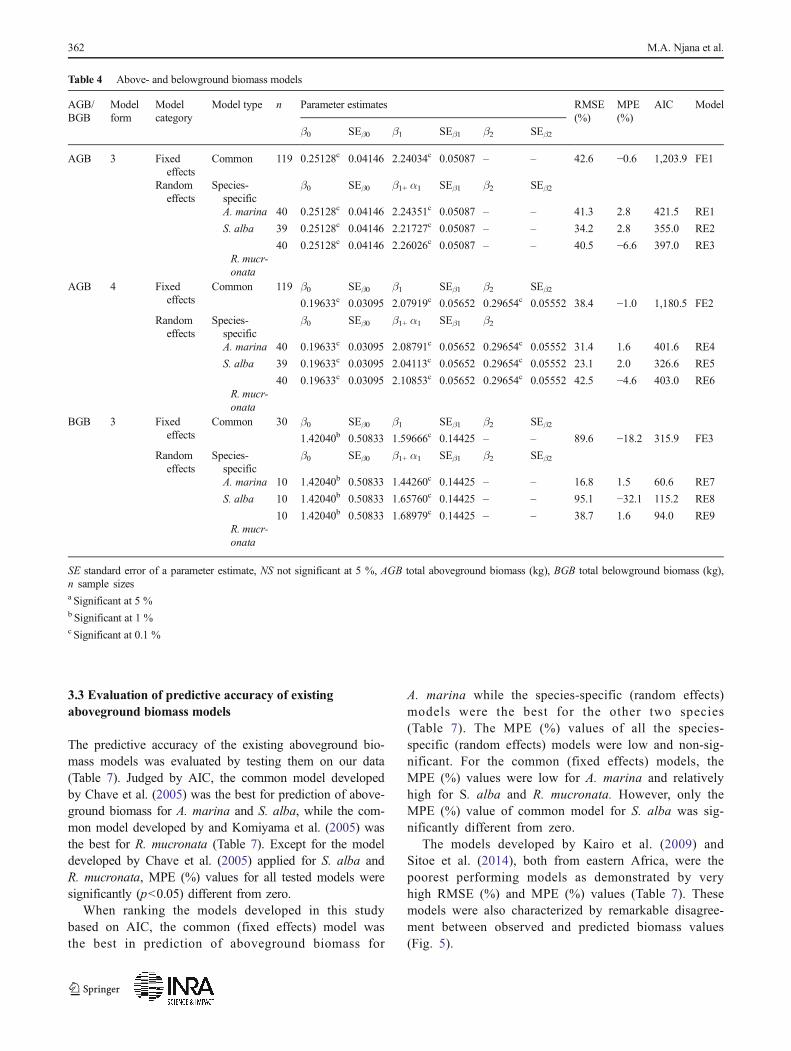
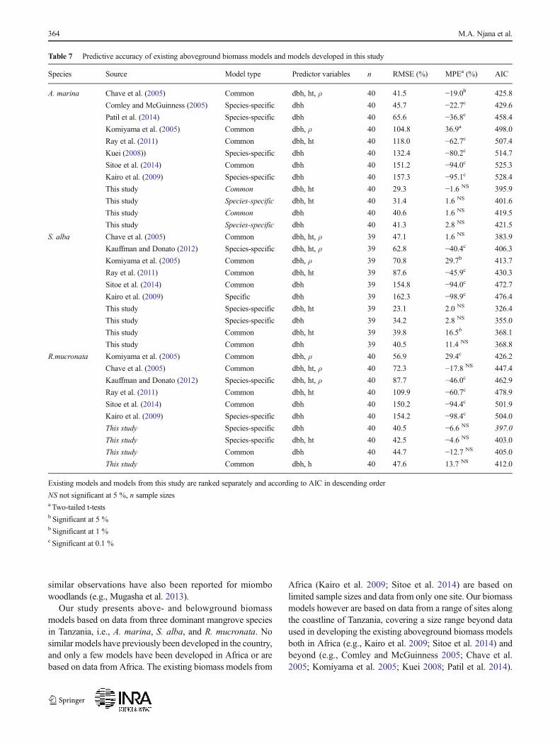
The predictive accuracy of the existing aboveground bio-mass models was evaluated by testing them on our data(Table 7). Judged by AIC, the common model developedby Chave et al. (2005) was the best for prediction of above-ground biomass for A. marina and S. alba, while the com-mon model developed by and Komiyama et al. (2005) wasthe best for R. mucronata (Table 7). Except for the modeldeveloped by Chave et al. (2005) applied for S. alba andR. mucronata, MPE (%) values for all tested models weresignificantly (p<0.05) different from zero.

When ranking the models developed in this studybased on AIC, the common (fixed effects) model wasthe best in prediction of aboveground biomass for

A. marina while the species-specific (random effects)models were the best for the other two species(Table 7). The MPE (%) values of all the species-specific (random effects) models were low and non-sig-nificant. For the common (fixed effects) models, theMPE (%) values were low for A. marina and relativelyhigh for S. alba and R. mucronata. However, only theMPE (%) value of common model for S. alba was sig-nificantly different from zero.

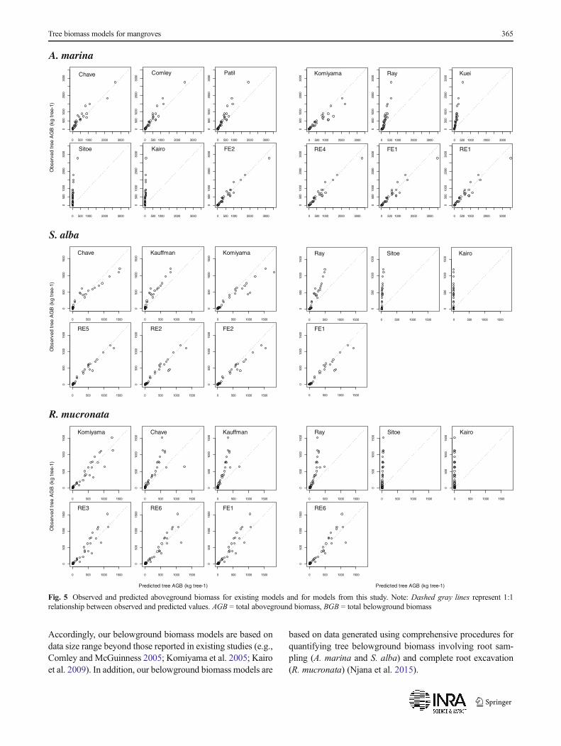
The models developed by Kairo et al. (2009) andSitoe et al. (2014), both from eastern Africa, were thepoorest performing models as demonstrated by veryhigh RMSE (%) and MPE (%) values (Table 7). Thesemodels were also characterized by remarkable disagree-ment between observed and predicted biomass values(Fig. 5).

Table 4 Above- and belowground biomass models

AGB/BGB

Modelform

Modelcategory

Model type n Parameter estimates RMSE(%)

MPE(%)

AIC Model

β0 SEβ0 β1 SEβ1 β2 SEβ2

AGB 3 Fixedeffects

Common 119 0.25128c 0.04146 2.24034c 0.05087 – – 42.6 −0.6 1,203.9 FE1

Randomeffects

Species-specific

β0 SEβ0 β1+ α1 SEβ1 β2 SEβ2

A. marina 40 0.25128c 0.04146 2.24351c 0.05087 – – 41.3 2.8 421.5 RE1

S. alba 39 0.25128c 0.04146 2.21727c 0.05087 – – 34.2 2.8 355.0 RE2

R. mucr-onata

40 0.25128c 0.04146 2.26026c 0.05087 – – 40.5 −6.6 397.0 RE3

AGB 4 Fixedeffects

Common 119 β0 SEβ0 β1 SEβ1 β2 SEβ2

0.19633c 0.03095 2.07919c 0.05652 0.29654c 0.05552 38.4 −1.0 1,180.5 FE2

Randomeffects

Species-specific

β0 SEβ0 β1+ α1 SEβ1 β2

A. marina 40 0.19633c 0.03095 2.08791c 0.05652 0.29654c 0.05552 31.4 1.6 401.6 RE4

S. alba 39 0.19633c 0.03095 2.04113c 0.05652 0.29654c 0.05552 23.1 2.0 326.6 RE5

R. mucr-onata

40 0.19633c 0.03095 2.10853c 0.05652 0.29654c 0.05552 42.5 −4.6 403.0 RE6

BGB 3 Fixedeffects

Common 30 β0 SEβ0 β1 SEβ1 β2 SEβ2

1.42040b 0.50833 1.59666c 0.14425 – – 89.6 −18.2 315.9 FE3

Randomeffects

Species-specific

β0 SEβ0 β1+ α1 SEβ1 β2 SEβ2

A. marina 10 1.42040b 0.50833 1.44260c 0.14425 – – 16.8 1.5 60.6 RE7

S. alba 10 1.42040b 0.50833 1.65760c 0.14425 – – 95.1 −32.1 115.2 RE8

R. mucr-onata

10 1.42040b 0.50833 1.68979c 0.14425 – – 38.7 1.6 94.0 RE9

SE standard error of a parameter estimate, NS not significant at 5 %, AGB total aboveground biomass (kg), BGB total belowground biomass (kg),n sample sizesa Significant at 5 %b Significant at 1 %c Significant at 0.1 %

362 M.A. Njana et al.

4 Discussion

The distributions of the aboveground biomass componentswere quite similar for A. marina and R. mucronata, while forS. alba, the proportion of stem biomass was higher than for thetwo other species (Fig. 3). Although on average 41 % of treebiomass was stored belowground, S. alba stored the largestproportion belowground (Fig. 4). The main reason for the rel-atively large proportion of belowground biomass for S. alba, ascompared to A. marina, is probably due to the large pneumat-ophores of this species (Njana et al. 2015). This is also in line

with the high root-to-shoot ratio for this species. Apparently,S. alba has more belowground biomass than aboveground bio-mass (1.29 root-to-shoot ratio). Variation of distribution of bio-mass into different tree components between species and adeclining trend in root-to-shoot ratios over dbh classes demon-strate the strategies of trees as they grow; at early stages, morebiomass is distributed in the belowground for anchorage andstabilization in the soft substrate, while at later stages, more ofthe biomass is distributed to the aboveground part in support ofphysiological processes for growth. The distribution of biomassobserved in this study is not unique for mangrove alone as

Table 5 Mean prediction errors (MPE (%)) of the aboveground biomass models over site, dbh class, and ht class

Parameter n MPE (%)

Model form 3 Model form 4

Fixed effects model Random effects model Fixed effects model Random effects model

Site

Pangani 15 −4.4 −2.2 −9.1 4.6

Bagamoyo 45 7.3 8.2 −2.9 −1.3Rufiji 45 −9.5 −10.7 2.2 −0.0Lindi-Mtwara 15 20.8 22.9 5.0 8.8

dbh class (cm)

1.0–10.0 45 12.8 12.6 10.3 9.8

10.1–20.0 20 −3.2 −3.6 −2.7 −2.920.1–30.0 20 −4.7 −3.4 −5.5 −3.830.1–40.0 24 −1.4 −0.7 −1.2 0.1

40.0 10 2.0 1.8 1.1 0.8

ht class (m)

1.0–5.0 24 10.2 11.7 −10.8 −9.55.1–10.0 36 25.2 24.7 8.4 7.9

10.1–15.0 29 4.7 6.7 −3.6 −0.215.1–20.0 14 −15.1 −12.0 −14.8 −9.5>20.0 16 −3.2 −6.8 11.8 5.6

n sample sizes

Table 6 Aboveground tree component biomass models

Component Model form Model category Model type n Parameter estimates RMSE (%) MPE (%) AIC Model

β0 SEβ0 β1 SEβ1

Leaf 3 Fixed effects Common 55 0.91766NS 0.64173 1.04996c 0.20549 62.1 8.2 367.8 CFE1

Twig 3 Fixed effects Common 55 0.83391NS 0.65931 1.35324c 0.23032 68.2 8.7 496.9 CFE2

Branch 3 Fixed effects Common 55 0.05140NS 0.05060 2.28062c 0.27769 78.0 −8.4 598.5 CFE3

Stem 3 Fixed effects Common 55 0.24370a 0.11111 2.06187c 0.13711 49.9 −11.4 641.2 CFE4

SE standard error of a parameter estimate, NS not significant at 5 %, n sample sizesa Significant at 5 %b Significant at 1 %c Significant at 0.1 %

Tree biomass models for mangroves 363

similar observations have also been reported for miombowoodlands (e.g., Mugasha et al. 2013).

Our study presents above- and belowground biomassmodels based on data from three dominant mangrove speciesin Tanzania, i.e., A. marina, S. alba, and R. mucronata. Nosimilar models have previously been developed in the country,and only a few models have been developed in Africa or arebased on data from Africa. The existing biomass models from

Africa (Kairo et al. 2009; Sitoe et al. 2014) are based onlimited sample sizes and data from only one site. Our biomassmodels however are based on data from a range of sites alongthe coastline of Tanzania, covering a size range beyond dataused in developing the existing aboveground biomass modelsboth in Africa (e.g., Kairo et al. 2009; Sitoe et al. 2014) andbeyond (e.g., Comley and McGuinness 2005; Chave et al.2005; Komiyama et al. 2005; Kuei 2008; Patil et al. 2014).

Table 7 Predictive accuracy of existing aboveground biomass models and models developed in this study

Species Source Model type Predictor variables n RMSE (%) MPEa (%) AIC

A. marina Chave et al. (2005) Common dbh, ht, ρ 40 41.5 −19.0b 425.8

Comley and McGuinness (2005) Species-specific dbh 40 45.7 −22.7c 429.6

Patil et al. (2014) Species-specific dbh 40 65.6 −36.8c 458.4

Komiyama et al. (2005) Common dbh, ρ 40 104.8 36.9a 498.0

Ray et al. (2011) Common dbh, ht 40 118.0 −62.7c 507.4

Kuei (2008)) Species-specific dbh 40 132.4 −80.2c 514.7

Sitoe et al. (2014) Common dbh 40 151.2 −94.0c 525.3

Kairo et al. (2009) Species-specific dbh 40 157.3 −95.1c 528.4

This study Common dbh, ht 40 29.3 −1.6 NS 395.9

This study Species-specific dbh, ht 40 31.4 1.6 NS 401.6

This study Common dbh 40 40.6 1.6 NS 419.5

This study Species-specific dbh 40 41.3 2.8 NS 421.5

S. alba Chave et al. (2005) Common dbh, ht, ρ 39 47.1 1.6 NS 383.9

Kauffman and Donato (2012) Species-specific dbh, ht, ρ 39 62.8 −40.4c 406.3

Komiyama et al. (2005) Common dbh, ρ 39 70.8 29.7b 413.7

Ray et al. (2011) Common dbh, ht 39 87.6 −45.9c 430.3

Sitoe et al. (2014) Common dbh 39 154.8 −94.0c 472.7

Kairo et al. (2009) Specific dbh 39 162.3 −98.9c 476.4

This study Species-specific dbh, ht 39 23.1 2.0 NS 326.4

This study Species-specific dbh 39 34.2 2.8 NS 355.0

This study Common dbh, ht 39 39.8 16.5b 368.1

This study Common dbh 39 40.5 11.4 NS 368.8

R.mucronata Komiyama et al. (2005) Common dbh, ρ 40 56.9 29.4c 426.2

Chave et al. (2005) Common dbh, ht, ρ 40 72.3 −17.8 NS 447.4

Kauffman and Donato (2012) Species-specific dbh, ht, ρ 40 87.7 −46.0c 462.9

Ray et al. (2011) Common dbh, ht 40 109.9 −60.7c 478.9

Sitoe et al. (2014) Common dbh 40 150.2 −94.4c 501.9

Kairo et al. (2009) Species-specific dbh 40 154.2 −98.4c 504.0

This study Species-specific dbh 40 40.5 −6.6 NS 397.0

This study Species-specific dbh, ht 40 42.5 −4.6 NS 403.0

This study Common dbh 40 44.7 −12.7 NS 405.0

This study Common dbh, h 40 47.6 13.7 NS 412.0

Existing models and models from this study are ranked separately and according to AIC in descending order

NS not significant at 5 %, n sample sizesa Two-tailed t-testsb Significant at 5 %b Significant at 1 %c Significant at 0.1 %

364 M.A. Njana et al.

Accordingly, our belowground biomass models are based ondata size range beyond those reported in existing studies (e.g.,Comley and McGuinness 2005; Komiyama et al. 2005; Kairoet al. 2009). In addition, our belowground biomass models are

based on data generated using comprehensive procedures forquantifying tree belowground biomass involving root sam-pling (A. marina and S. alba) and complete root excavation(R. mucronata) (Njana et al. 2015).

A. marina

S. alba

R. mucronata

0 500 1000 2000 3000

050

010

0020

0030

00

Chave

0 500 1000 2000 3000

050

010

0020

0030

00

Comley

0 500 1000 2000 3000

050

010

0020

0030

00

Patil

0 500 1000 2000 3000

050

010

0020

0030

00

Sitoe

0 500 1000 2000 3000

050

010

0020

0030

00

Kairo

0 500 1000 2000 3000

050

010

0020

0030

00

FE2

Obs

erve

d tr

ee A

GB

(kg

tre

e-1)

0 500 1000 2000 3000

050

010

0020

0030

00

Komiyama

0 500 1000 2000 3000

050

010

0020

0030

00

Ray

0 500 1000 2000 3000

050

010

0020

0030

00

Kuei

0 500 1000 2000 3000

050

010

0020

0030

00

RE4

0 500 1000 2000 3000

050

010

0020

0030

00

FE1

0 500 1000 2000 3000

050

010

0020

0030

00

RE1

0 500 1000 1500

050

010

0015

00

Chave

0 500 1000 1500

050

010

0015

00

Kauffman

0 500 1000 1500

050

010

0015

00

Komiyama

0 500 1000 1500

050

010

0015

00

RE5

0 500 1000 1500

050

010

0015

00

RE2

0 500 1000 1500

050

010

0015

00

FE2

Obs

erve

d tr

ee A

GB

(kg

tre

e-1)

0 500 1000 1500

050

010

0015

00

Ray

0 500 1000 1500

050

010

0015

00

Sitoe

0 500 1000 1500

050

010

0015

00

Kairo

0 500 1000 1500

050

010

0015

00

FE1

0 500 1000 1500

050

010

0015

00

Komiyama

0 500 1000 1500

050

010

0015

00

Chave

0 500 1000 1500

050

010

0015

00

Kauffman

0 500 1000 1500

050

010

0015

00

RE3

0 500 1000 1500

050

010

0015

00

RE6

0 500 1000 1500

050

010

0015

00

FE1

Predicted tree AGB (kg tree-1)

Obs

erve

d tr

ee A

GB

(kg

tre

e-1)

0 500 1000 1500

050

010

0015

00

Ray

0 500 1000 1500

050

010

0015

00

Sitoe

0 500 1000 1500

050

010

0015

00

Kairo

0 500 1000 1500

050

010

0015

00

RE6

Predicted tree AGB (kg tree-1)

Fig. 5 Observed and predicted aboveground biomass for existing models and for models from this study. Note: Dashed gray lines represent 1:1relationship between observed and predicted values. AGB = total aboveground biomass, BGB = total belowground biomass

Tree biomass models for mangroves 365

Our models are based on a nonlinear mixed-modelling ap-proach. Ordinary nonlinear regression is commonly used todevelop biomass models. Such models, however, may violateregression assumptions of homoscedast ici ty andindependence of residuals, which are difficult to meet forbiological data. Sampling for biomass model developmentoften results in hierarchical data. Chave et al. (2005) andKomiyama et al. (2005) for example developed common bio-mass models using data originating from more than one site,such data form hierarchical data structure stratified by site andspecies. Observations originating from the same species andor site are likely to be more correlated hence lack of indepen-dence. A model based on non-independent observations ischaracterized by autocorrelated errors and therefore violatekey assumptions of independence in regression (Ritz andStreibig 2008). Ignoring lack of independence tends to giveimprecise parameter estimates (ibid.). The mixed effectsmodelling comprising both fixed and random effects that weapplied in this study is a useful statistical tool in modellinghierarchical data (Ritz and Streibig 2008; Zuur et al. 2009).

Our study showed that the aboveground biomass modelsimproved when random effects modelling was applied andwhen ht as an additional predictor variable was considered(Tables 4 and 5). In model development, it is important thatmodels are properly specified and that the structure of the datais taken into account. Our study illustrate that common modelincluding ht generally performed well across study site, spe-cies, dbh, and ht classes by resulting into decline in MPE (%)and that their corresponding random effects/species-specificfurther improved predictive accuracy (Table 5). This supportsthe role of random effects in explaining unexplained sourcesof variation which is only possible within the mixed model-ling framework. In line with our results, Chave et al. (2005)reported that the inclusion of ht into a common mangrovebiomass model reduced the standard error of abovegroundbiomass from 19.5 to 12.5 % for mangrove trees, while otherauthors reported that random effects improved predictivepower of biomass models for non-mangrove trees (e.g., Fuet al. 2014; Xu et al. 2014).

Despite models including ht being better, in most forestinventories, due to many reasons such as costs, trees are notfrequently measured for ht. In such cases, users are obligedeither to use models including dbh as the only predictor var-iable or initially estimate ht using relevant models and subse-quently apply biomass models based on both dbh and ht aspredictor variables. However, ht prediction models for man-groves are lacking in Tanzania and the rest of Africa.

Basic density (BD) is another predictor variable whichcould have potentially improved predictive accuracy particu-larly for the common biomass model (Komiyama et al. 2005;Chave et al. 2005). However, our models did not include BDas an additional predictor variable for two reasons; firstly, BDmay vary between species and between species-specific tree

components and between tree size. Therefore, applying BDdetermined based on comprehensive sampling in modellingtree biomass may improve model predictive accuracy. SinceBD is never determined in forest inventories however and thatno BD prediction models exist for mangrove species, suchbiomass models would be better yet with limited application.Secondly, for common biomass models, BD serves as speciesdistinguishing factor whereby species mean BD values maybe used as opposed to the use of species- and tree-specific BDvalues. The mixed modelling approach used in this study isrobust in distinguishing species.

The tests of existing models on our data generally showedlarge and significant underpredictions for aboveground bio-mass (Table 7). The underpredictions were as large as 90 %for some of the models (Kairo et al. 2009; Sitoe et al. 2014).Generally, predicted and observed biomass agreed quite wellfor small tree sizes, while the underpredictions increased withtree size (Fig. 5). Similar tests on belowground biomass formangroves in Tanzania (Njana et al. 2015) showed predictionerrors (underprediction) as high as 60 % when models byKomiyama et al. (2005) (common model), Comley andMcGuinness (2005) (species-specific model), and Kairoet al. (2009) (species-specific model) were applied. Plausibleexplanations for the observed prediction errors could be theapplication of the models beyond data ranges (size), geo-graphical locations, and differences in forest structure andarchitecture. For the belowground biomass, an additional ex-planation could also be inadequate excavation procedures ap-plied when some of these models were developed (see Njanaet al. 2015). Any application of the already existing above-and belowground biomass models to mangroves of Tanzaniais therefore not recommended.

In the modelling, we applied species as random effects,which resulted into improved predictive accuracy of both theabove- and the belowground biomass models, except for be-lowground biomass for S. alba where the models did not fitwell to data (Table 4). This may be due to higher variances ofBGB for this species (see Fig. 2). The contribution of randomeffects in improved predictive accuracy suggests that the bio-mass allometry varies by species. Therefore, the randomeffects/species-specific models should be applied since theyare superior to the fixed effects/common models. For S. alba,however, the fixed effects model is recommended for below-ground biomass. Since both the above- and the belowgroundbiomass models performed fairly well across sites, the modelsmay be applied across sites in Tanzania. However, the use ofthe models beyond species considered in this study is notrecommended.

Aboveground tree component biomass estimates derivedusing models may be essential in describing forest structure(e.g., Camacho et al. 2011), determining forest productivity(e.g., Cox and Allen 1999; Kairo et al. 2008), and understand-ing ecosystem functions through quantification of carbon

366 M.A. Njana et al.

stocks and sequestration (e.g., Chen et al. 2012; Pandey andPandey 2013) which are potentially relevant for climatechange mitigation strategies. For example, the leaf biomassestimated from relevant models may provide useful informa-tion on nutrient cycling while the above- and belowgroundbiomass models may be applied to generate tier 3 carbon stockestimates for carbon monitoring, reporting, and verification inREDD+ programs. The models may also be applied to theNAFORMA data for basic scientific ecological studies andfor management decision-making. Since biomass estimatesare essential for both ecological and management applica-tions, the models (total AGB, BGB, and tree componentmodels) from this study are expected to provide ecologistswith the needed information and to support management ofmangroves in Tanzania and elsewhere as deemed relevant.The aboveground tree component biomass models that wedeveloped generally gave low prediction errors (<10 %)(Table 6). In addition, estimates based on tree componentswere additive (in agreement with the direct tree abovegroundestimates). Therefore, we recommend the use of the developedaboveground tree component common models in derivingaboveground component-specific biomass estimates for utili-zation and ecological purposes, and the individual estimatesmay safely be added up.

5 Conclusions

The biomass models reported in this study are based on com-prehensive data and modelling approach. The above- and be-lowground biomass models improved when random effectswere considered. Therefore, random effects/species-specificmodels are generally recommended. For estimation of below-ground biomass for S. alba however, the fixed effects/common model is recommended. Based on our results, wediscourage species-specific or site-specific model develop-ment for data entailing more than one species or site, insteadwe encourage the use of a mixed modelling approach which isrobust for such data sets. The aboveground tree componentbiomass models may also be applied since they yield unbiasedand additive estimates. Based on goodness of fit statistics,both the above- and the belowground biomass models devel-oped in this study are the best available and provide an im-portant tool for accurate estimation of biomass and carbonstock stored in mangrove forest in Tanzania for both manage-ment and ecological applications. Our models should be usedwithin the range of data from which they were developed, andtheir use outside this data range should be done with caution.

Acknowledgments We thank the Tanzania Forest Service (TFS) fieldofficers D. Mnyagi (Pangani), S. K. Nyabange (Bagamoyo), H. Mallya(Rufiji), andM. C. Mbago (Mtwara) for facilitation and logistical supportduring field work. We appreciate field assistants and the boat driver for

their enthusiasm, hard work, courage, and encouragement during an in-tensive and risky fieldwork. The authors also would like to thank Tanza-nia Forest Service for permitting destructive sampling of mangrove treesfor this study.

Funding We gratefully acknowledge financial support from theClimate Change Impacts and Adaptation Mitigation (CCIAM)Programme. The financial support from research projects, Impact of cli-mate change on mangrove ecosystems and associated fishery resourcesalong the Tanzanian coast and enhancing the Measuring, Reporting andVerification (MRV) of forests in Tanzania, is also appreciated.We are alsoindebted to CCIAM Programme for a PhD scholarship to the first author.

References

Brown S (1997) Estimating biomass change of tropical forests: primer,FAO Forestry Paper 134, Rome, Italy

Burnham KP, Anderson DR, Huyvaert KP (2011) AIC model selectionand multi-model inference in behavioural ecology: some back-ground, observations, and comparisons. Behav Ecol Sociol Biol65:23–35

Camacho LD, GevañaDT, Carandang AP, Camacho SC, Combalicer AE,Rebugio LL, Youn Y (2011) Tree biomass and carbon stock of acommunity‐managedmangrove forest in Bohol, Philippines. For SciTechnol 7:161–167

Chai T, Draxler RR (2014) Root mean square error (RMSE) or meanabsolute error (MAE)?—arguments against avoiding RMSE in theliterature. Geosci Model Dev 7:1247–1250

Chave J, Andalo C, Brown S, Cairns MA, Chambers JQ, Eamus D,Fölster H, Fromard F, Higuchi N, Kira T, Lescure JP, Nelson B,Ogawa H, Puig H, Riéra B, Yamakura T (2005) Tree allometryand improved estimation of carbon stocks and balance in tropicalforests. Oecologia 145:87–99

Chave J, Rejou-MechainM, Burquez A, Chidumayo E, ColganMS, DelittiWBC, Duque A, Eid T, Fearnside PM, Goodman RC, Henry M,Martinez-Yrizar A, Mugasha W, Muller-Landau HC, MencucciniM, Nelson BW, Ngomanda A, Nogueira EM, Ortiz-Malavassi E,Pelissier R, Ploton P, Ryan CM, Saldarrriaga JG, Vieilledent (2014)Improved allometric models to estimate the aboveground biomass oftropical trees. Glob Chang Biol 10:3177–3190

Chen L, Zeng X, Tam NFY, Lu W, Luo Z, Du X, Wang J (2012)Comparing carbon sequestration and stand structure of monocultureand mixed mangrove plantations of Sonneratia caseolaris andS. apetala in Southern China. For Ecol Manag 284:222–229

Comley BWT, McGuinness KA (2005) Above- and below-ground bio-mass, and allometry of four common northern Australian man-groves. Aust J Bot 53:431–436

R Core Team (2014) R: a language and environment for statistical com-puting. R Foundation for Statistical Computing, Vienna, Austria.http://cran.r-project.org/bin/windows/base/ Accessed 20 Nov 2014

Cox EF, Allen JA (1999) Stand structure and productivity of the intro-duced Rhizophora mangle in Hawaii. Estuaries 22:276–284

de Miguel S, Pukkala T, Assaf N, Shater Z (2014) Intra-specific differ-ences in allometric equations for aboveground biomass of EasternMediterranean Pinus brutia. Ann For Sci 71:101–112

Donato DC, Kauffman JB, Murdiyarso D, Kurnianto S, Stidham M,Kanninen M (2011) Mangroves among the most carbon-rich forestsin the tropics. Nat Geosci 4:293–297

FAO (2007) The world’s mangroves 1980-2005. FAO Forestry Paper153, Rome, FAO

Fatoyinbo TE, Simard M, Washington-Allen RA, Shugart H (2008)Landscape-scale extent, height, biomass, and carbon estimation of

Tree biomass models for mangroves 367

Mozambique’s mangrove forests with Landsat ETM+ and ShuttleRadar Topography Mission elevation data. Geophys Res 113:1–14

Fu L, Zeng W, Zhang H, Wang G, Lei Y, Tang S (2014) Generic linearmixed-effects individual-tree biomass models for Pinus massonianain Southern China. South For 76:47–56

Harrell FE (2001) Regression modelling strategies: with application tolinear models, logistic regression and survival analysis. Springer,New York

Hewson J, Steininger M, Pesmajoglou S (2013) REDD+ Measurement,Reporting and Verification (MRV)manual. USAID-supported forestcarbon. Markets and Communities Program, Washington, DC

Husch B, Beers TW, Kershaw JA (2003) Forest mensuration, 4th edn.Wiley and Sons, Inc., Canada

IPCC (2003) IPCC good practice guidance for LULUCF. Institute forGlobal Environmental Strategies (IGES) for the IPCC. Kanagawa,Japan, p 590

IPCC (2006) Guidelines for national greenhouse gas inventories. IGES,Japan

IPCC (2007) Fourth assessment report: climate change 2007 (AR4)<http://www.ipcc.ch/publications_and_data/publications_and_data_reports.htm#1>

Johnson JB, Omland KS (2004) Model selection in ecology and evolu-tion. Trends Ecol Evol 19:101–108

Kairo JG, Lang’at JKS, Dahdouh-Guebas F, Bosire J, Karachi M (2008)Structural development and productivity of replanted mangroveplantations in Kenya. For Ecol Manag 255:2670–2677

Kairo JG, Bosire J, Langat J, Kirui B, Koedam N (2009) Allometry andbiomass distribution in replanted mangrove plantations at Gazi Bay,Kenya. Aquat Conserv 19:S63–S69

Kauffman JB, Donato DC (2012) Protocols for the measurement, moni-toring and reporting of structure, biomass and carbon stocks in man-grove forests. Working Paper 86. CIFOR, Bogor, Indonesia

Komiyama A, Poungparn S, Kato S (2005) Common allometric equationsfor estimating the tree weight of mangroves. J Trop Ecol 21:471–477

Komiyama A, Ong JE, Poungparn S (2008) Allometry, biomass, andproductivity of mangrove forests: a review. Aquat Bot 89:128–137

Kuei CF (2008) Population structure, allometry and above-ground bio-mass of Avicennia marina forest at the Chishui River Estuary,Tainan County, Taiwan. J For Res 30:1–16

Li Y, Jiang L, Liu M (2011) A nonlinear mixed-effects model to predictstem cumulative biomass of standing trees. Procedia Environ Sci 10:215–221

Lindstrom MJ, Bates DM (1990) Nonlinear mixed effects models forrepeated measures data. Biometrics 46:673–687

Luoga EJ, Malimbwi RE, Kajembe GC, Zahabu E, Shemwetta DTK,Lyimo-Macha J, Mtakwa P, Mwaipopo CS (2004) Tree speciescomposition and structures of Jasini Mwajuni Mangrove forest atPangani, Tanzania. J TAF10:42–47

MNRT (Ministry of Natural Resources and Tourism) (1991)Management plan for the mangrove ecosystem of Rufiji District,mainland Tanzania, vol 7. Ministry of Tourism, Natural Resourcesand Environment (MTNRE), Forestry and Beekeeping Division,Catchment Forestry Project, Dar es Salaam

MNRT (Ministry of Natural Resources and Tourism) (2015) NAFORMA(National Forest Monitoring and Assessments of Tanzania) mainresults. Dar es Salaam

MohamedMOS, Neukermans G, Kairo JG, Dahdouh-Guebas F, KoedamN (2009) Mangrove forests in a peri-urban setting: the case ofMombasa (Kenya). Wetl Ecol Manag 17:243–255

Moore JR (2010) Allometric equations to predict the total above-groundbiomass of radiata pine trees. Ann For Sci 67:806–817

Mattia SB (1997) Species and structural composition of natural mangroveforests: a case study of the Rufiji delta, Tanzania. Dissertation foraward of MSc. Degree at Sokoine University of Agriculture,Morogoro, Tanzania

Mugasha WA, Eid T, Bollandsås OM, Malimbwi RE, Chamshama SAO,Zahabu E, Katani JZ (2013) Allometric models for prediction ofabove- and belowground biomass of trees in the miombowoodlandsof Tanzania. For Ecol Manag 310:87–101

Murray B, Pendleton L, JenkinsWA, Sifleet S (2011) Green payments forblue carbon economic incentives for protecting threatened coastalhabitats, report NI 11 04. Institute for Environmental PolicySolutions, Nicholas

Njana MA, Eid T, Zahabu E, Malimbwi R (2015) Procedures for quanti-fication of belowground biomass of three mangrove tree species.Wetl Ecol Manag 23:749–764

Nshare JS, Chitiki A, Malimbwi RE, Kinana BM, Zahabu E (2007) Thecurrent status of the mangrove forest along seashore at Salendabridge, Dar es Salaam, Tanzania. J TAF 11:172–179

O’Hara RB, Kotze DJ (2010) Do not log-transform count data. MethodsEcol Evol 1:118–122

Packard GC (2009) On the use of logarithmic transformations in allome-tric analyses. J Theor Biol 257:515–518

Pandey CN, Pandey R (2013) Carbon sequestration by mangroves ofGujarat. India Int Jof Bot 3:57–70

Patil V, Singh A, Naik N, Unnikrishnan S (2014) Estimation of carbonstocks in Avicennia marina stand using allometry, CHN analysis,and GIS methods. Wetlands 34:379–391

Pinheiro J, Bates DM (1998) Model building for nonlinear mixed effectsmodel. Department of Statistics University of Wisconsin, Madison

Pinheiro J, Bates D (2000) Mixed effects models in S and S-PLUS.Springer, New York

Pinheiro J, Bates D, DebRoy S, Sarkar D, R Core Team (2015) nlme:linear and nonlinear mixed effects models. R package version 3.1-119, http://CRAN.R-project.org/package=nlme

Ray R, Ganguly D, Chowdhury C, Dey M, Das S, Dutta MK, MandalSK, Majumder N, De TK, Mukhopadhyay JTK (2011) Carbon se-questration and annual increase of carbon stock in mangrove forest.Atmos Environ 45:5016–5024

Ritz C, Streibig JC (2008) Nonlinear regression with R. Springer, New YorkRoxburgh SH, Paul KI, Clifford D, England JR, Raison RJ (2015)

Guidelines for constructing allometric models for the prediction ofwoody biomass: how many individuals to harvest? Ecosphere 6:38.doi:10.1890/ES14-00251.1

Sileshi GW (2014) A critical review of forest biomass estimation models,common mistakes and corrective measures. For Ecol Manag 329:237–254

Sitoe AA, Mandlate LJC, Guedes BS (2014) Biomass and carbon stocksof Sofala bay mangrove forests. Forests 5:1967–1981

Smith A, Granhus A, Astrup R, Bollandsås OM, Petersson H (2014)Functions for estimating aboveground biomass of birch inNorway. Scand J For Res 29:565–578

Tamai S, Nakasuga T, Tabuchi R, Ogino K (1986) Standing biomass ofmangrove forests in Southern Thailand. J Jpn For Soc 68:384–388

Tamooh F, Huxhamd M, Karachi M, Mencuccini M, Kairo JG, Kirui B(2008) Below-ground root yield and distribution in natural andreplanted mangrove forests at Gazi Bay, Kenya. For Ecol Manag256:1290–1297

UNEP (UnitedNations Environment Programme) (2014) The importanceof mangroves to people: a call to action. van Bochove, J., Sullivan,E., Nakamura, T. (Eds). United Nations Environment ProgrammeWorld Conservation Monitoring Centre, Cambridge. 128 pp

URT (United Republic of Tanzania) (2002) The Forest Act No. 14.Forestry and Beekeeping Division, Ministry of Natural Resourcesand Tourism. Dar es Salaam, Tanzania. 281 pp

URT (United Republic of Tanzania) (2010) National Forest ResourcesMonitoring and Assessment of Tanzania (NAFORMA). Field man-ual. Biophysical survey. NAFORMA document M01–2010, p. 108

Vonesh EF, Chinchilli VM (1997) Linear and nonlinear models for theanalysis of repeated measurements. Marcel Dekker, Inc., New York

368 M.A. Njana et al.

Walther BA, Moore JL (2005) The concepts of bias, precision and accu-racy, and their use in testing the performance of species richnessestimators, with a literature review of estimator performance.Ecography 28:815–829

Wang Y, Bonynge G, Nugranad J, TraberM, Ngusaru A, Tobey J, Hale L,Bowen R, Makota V (2003) Remote sensing of mangrove changealong the Tanzania coast. Mar Geod 26:1–14

West BT,Welch KB, Gałecki AT (2007) Linear mixed models: a practicalguide using statistical software. Taylor and Francis Group, LLC,New York

Xu H, Sun Y, Wang X, Fu Y, Dong Y (2014) Nonlinear mixed-effects(NLME) diameter growth models for individual China-fir(Cunninghamia lanceolata) trees in Southeast China. PLoS ONE9:e104012. doi:10.1371/journal.pone.0104012

Zhou X, Brandle JR, Schoeneberger MM, Awada T (2007) Developingabove-ground woody biomass equations for open-grown, multiple-stemmed tree species: shelterbelt-grown Russian-olive. Ecol Model202:311–323

Zuur A, Ieno EN, Walker NJ, Saveliev AA, Smith GM (2009) Mixedeffects models and extensions in ecology with R. Springer, New York

Tree biomass models for mangroves 369