APS/123-QED

A wireless interrogation system exploiting narrowband acoustic

resonator for remote physical quantity measurement

J.-M Friedt

SENSeOR

32, avenue de l’Observatoire,

25044 Besancon FRANCE∗

C. Droit, G. Martin, and S. Ballandras

FEMTO-ST, Time & frequency department

32, avenue de l’Observatoire, 25044 Besancon FRANCE

(Dated: October 29, 2009)

Abstract

Monitoring physical quantities using acoustic wave devices can be advantageously achieved us-

ing the wave characteristic dependence to various parametric perturbations (temperature, stress,

pressure). Surface Acoustic Wave (SAW) resonators are particularly well suited to such applica-

tions as their resonance frequency is directly influenced by these perturbations, modifying both

the phase velocity and resonance conditions. Moreover, the intrinsic radiofrequency (RF) nature

of these devices make them ideal for wireless applications, mainly exploiting antennas reciprocity

and piezoelectric reversibility. In this paper, we present a wireless SAW sensor interrogation unit

operating in the 434 MHz centered ISM band – selected as a tradeoff between antenna dimensions

and electromagnetic wave penetration in dielectric media – based on the principles of a frequency

sweep network analyzer. We particularly focus on the compliance with the ISM standard which re-

veals complicated by the need for switching from emission to reception modes similarly to RADAR

operation.

In this matter, we propose a fully digital RF synthesis chain to develop various interrogation

strategies to overcome the corresponding difficulties and comply with the above-mentioned stan-

dard. We finally assess the reader interrogation range, accuracy and dynamics.

PACS numbers: 43.60.Qv

Keywords: Surface acoustic wave, sensor, wireless, interrogation unit

1

I. BASIC PRINCIPLES

Continuous or periodic monitoring of the physical properties of industrial tools, build-

ings, environmental equipment etc ... provide the basic informations to replace preventive

maintenance with predictive maintenance reacting to any abnormal behavior of parts of the

system being monitored. However, maintenance of aging devices means embedding sensors

with life expectancies longer than that of the observed system. Furthermore, the parts of in-

terest are usually subject to harsh environmental conditions – corrosive environment, strong

magnetic field associated with high current densities or high voltages for instance – or mobile

or rotating parts. Hence, wired sensors are unsuitable since the connections are often the

weak point making the packaging fragile and unreliable on the long term. Battery powered

wireless silicon based sensors1 provide one solution with increasing life expectancy as lower

power sensors, microcontrolers and wireless communication interfaces are developed2,3. Yet,

this lifetime is still finite and limited by the available battery power. Environmental preser-

vation however claims for battery-less systems capable to limit pollution issues. Passive

CMOS sensors based on RFID technology provide short interrogation distance and poorer

temperature measurement range than those presented in this document4,5.

We here propose an alternative mean of monitoring chemical6,7 and physical properties8,9

(temperature10–14, pressure15–18, strain19, torque20, moisture level21,22) using passive sensors

(no embedded battery source) probed using a wireless RF link. The basic sensor principle

is based on disturbing the resonance frequency of a RF resonator23. We actually use surface

acoustic wave (SAW) devices made of a piezoelectric substrate – quartz in all the examples

described here – patterned with electrodes for receiving and emitting electromagnetic waves

converted to acoustic waves through the piezoelectric effect24.

We are interested on the one hand in operating a low frequency device due to the better

penetration of electromagnetic waves in dielectric substrates such as the ones the parts being

monitored are made of, as well as to the ease of the fabrication of the sensors made of larger

patterns when operating at lower frequency. On the other hand, high frequency provides

the means for reducing the sensor and antenna sizes.

Since we aim at complying with radiofrequency (RF) emission regulations, two main

frequency bands are usable in Europe: 434 MHz and 2450 MHz. The latter frequency band

is wide enough for the operation of acoustic reflective delay lines (so-called SAW tags25–32),

2

but the penetration depth of the electromagnetic wave is too poor to embed the sensor in

most dielectric substrates such as soil or polymers. We are hence interested in the 434 MHz

band, which however only provides a 1.7 MHz bandwidth, insufficient for interrogating delay

lines with dimensions smaller than 10 mm but allowing for SAW-resonator-based sensor

exploitation33–36.

Hence, we focus on an interrogation unit37 allowing the identification of the resonance

frequency of narrowband acoustic devices: resonators. Since we will focus on the interroga-

tion instrument, we will assume the availability of resonators with acoustic modes operating

within the 434 MHz band, with quality factors in the 10000±2000 range: our objective is

the identification of these resonance frequencies using means compatible with a wireless link,

and the conversion of these frequencies to the physical parameter affecting the resonator.

The strategy we have first selected for interrogating narrowband devices is a slow sweep

of a frequency source with a spectral response narrower than that of the resonator. This

strategy is similar to that used by network analyzers, although the wireless link induces an

additional constraint, namely the alternating emission and reception phases, similar to that

used in RADAR systems. The basic components we need are hence a versatile frequency

source, a radiofrequency power reception circuit, and switches for activating and deactivating

emission and reception phases during the interrogation cycles. We have selected a fully

software-controled strategy in which a central ARM738 microcontroler synchronizes all the

interrogation steps, from the frequency generation to the digitization of the RF power level

and post-processing of the spectra for identifying the resonance frequencies.

II. SENSOR DESIGN

Piezoelectric sensors provide an efficient means of storing energy transferred through a RF

link. Being intrinsically RF components, SAW resonators are compact and do not require

additional components for converting the measured quantity to a RF signal, even though

such schemes have been demonstrated with, for example, resonance frequency pulling by a

capacitive sensor34,39.

SAW resonators built on single crystal piezoelectric substrates exhibit parametric sen-

sitivities varying along the substrate’s crystal orientation and are hence suitable for the

design of temperature or stress sensors (and associated pressure and torque sensors). In

3

order to reduce the sensitivity of SAW to unwanted parameters, and to reduce requirements

on the local reference oscillator (section III A), we exploit a differential design in which the

frequencies of a reference resonator and a sensing resonator are both monitored40,41. This

particular sensor provides usable signals in the -20 oC to 150 oC range while keeping all

resonances within the 1.7 MHz ISM band range : the typical first order Temperature Co-

efficient of Frequency (TCF) is thus of the order of 10 kHz/oC (23 ppm/K). This TCF is

practically reduced to 2.5 kHz/oC (6 ppm/K) to account for the differential measurement

which is performed under the assumption of the ISM band division in two equal parts and

including manufacturing variability: this value will be used throughout this article.

This simple dual-resonator design however lacks the ability to identify the sensor: both

resonances are used for the measurement, and optimum resolution is achieved by using all the

available radiofrequency band for the measurement. Adding a resonance for an identification

step would strongly reduce the measurement accuracy: in all the following discussion, the

interrogation unit is only associated to a single sensor at any given measurement time.

III. FREQUENCY GENERATION

Generating RF signals with continuously tunable frequency is commonly performed by

two major techniques: frequency multiplication using a phase locked loop, and mixing42.

Both methods are compatible with a software control of the emitted frequency using a quartz-

controlled direct digital synthesizer (DDS). A 32-bit frequency control word generating a

34 MHz signal to be mixed with a 400 MHz reference provides sub-Hz accuracy, below the

long term stability of the local reference oscillator.

In order to reduce the number of components and the possible noise sources, we select

a DDS (Analog Devices AD9954) strategy in which the core clock fCK is naturally added

to the output frequency fout due to the basic principle of DDS components. This output is

band-pass filtered using a SAW filter, and amplified to reach the maximum allowed output

power of 10 dBm as measured during continuous emission. The need for mixing is hence

eliminated and the major phase noise source – the 400 MHz signal – is eliminated so that

the only phase noise source remains the oscillator powering the DDS (Fig. 2).

The phase noise of such a synthesis was measured at 435 MHz and provided the best

performance in the frequency range of interest - 100 Hz to 10 kHz from the carrier frequency

4

– when compared to a mixing strategy (400 MHz PLL output mixed with 35 MHz DDS

output) or a PLL multiplication strategy (54.375 MHz DDS output multiplied by 8).

A. Local oscillator stability issue

All timing signals are synthesized from a unique quartz crystal resonator. Typical crystal

oscillators provide ±10 to ±50 ppm stability over the industrial temperature range (-40 to

85oC), i.e. 0.2 to 0.8 ppm/K. In a single resonator configuration, the resonance frequency

change of the sensor is smaller than this reference oscillator noise: a temperature sensor

working over a 170 K range and complying with the 434 MHz-band ISM regulations dis-

plays a linear coefficient of 23 ppm/K, so that a 0.1 K accuracy requires a local oscillator

accuracy better than 3 ppm/K. Below such stability, the drift of the reference oscillator can-

not be distinguished from the frequency shift of the sensor due to a temperature variation

during a measurement: common reference oscillator drift is not negligible with respect to

the measured frequency variation associated with the physical quantity measurement.

One aspect of dual resonators including a reference is that the local oscillator drift affects

the measurement of both resonance frequencies: although the available ISM band frequency

range is halved, the frequency shift to be measured is now in the MHz range (half of the

available ISM band) rather than close to 434 MHz. The requirements on the local oscillator

stability are hence reduced to about 670 ppm over the temperature range, easily met by any

commercially available resonator. Furthermore, aging is assumed to affect in a similar trend

both resonators so that the difference frequency is harldy affected, while a single resonator

measurement requires periodic recalibration to assess aging associated drift.

On the other hand, if a single resonator scheme is selected, means of long term stabiliza-

tion of the local oscillator (GPS 1 PPS signal43,44, NTP timing protocols over the internet45)

are necessary to preserve the measurements accuracy over long time periods. Furthermore,

we have observed46 that frequency pulling due to antenna impedance variations associated

with the interrogation unit environment changes significantly affects a single resonance,

while under the assumption that in a two resonator setup both resonators exhibit the same

impedance, such pulling is eliminated during the differential measurement step.

5

IV. RADIO FREQUENCY POWER RECEPTION

A. Power reception

Wideband Identity/Quadrature (I/Q) demodulators and power detectors are commer-

cially available with cutoff frequencies well above 434 MHz. We use such detectors – for

example Analog Devices AD8362 – for direct power measurement after filtering and amplify-

ing the signal received by the antenna, switched towards the reception circuit. The bandpass

filtering is performed by a bandpass SAW filter so as to reject any signal outside the ISM

band. However, integrating the total power within the whole ISM band makes the detector

sensitive to unwanted signals, since unwanted emitters in the ISM band, which provide a

signal as strong as the returned signal from the loaded resonator, mask the wanted signal.

Furthermore, the RF receiver noise level increases with increasing reception frequency band-

width. We have nevertheless observed that the 60 dB dynamic range is enough to reach an

interrogation range of several meters (typically 3 m, 11 m at best) in free space.

An alternative scheme providing efficient demodulation and improved resistance to un-

wanted emitters, yet keeping the 60 dB dynamic range, is the use of I/Q demodulators, such

as Analog Devices AD8302.

The output of either magnitude signal from the I/Q demodulator or power detector is fed

to a fast, rail to rail operational amplifier configured as amplifier and subtractor for remov-

ing any offset generated by the RF stage. The output of the operational amplifier is directly

connected to the fast analog to digital converter of the microcontroler (1 Msamples/s). The

control of all sequences by this same processor guarantees the best synchronization of the

switch commutation followed by a fast sampling of the received power: the resulting magni-

tude is associated with the frequency that was programmed in the DDS during this same se-

quence. No frequency uncertainty between a slowly, continuously, varying voltage controlled

oscillator (VCO) and the sampling time is introduced with this scheme. A 1 Msamples/s

analog to digital converter is fast enough to process the power detector output of a 434 MHz

resonator with a quality factor Q of 10000 since the decay time after loading the resonator

is Q/π periods, equal to about 6 µs. This scheme is however no longer applicable to higher

frequency resonators (with lower Q-factor assuming a constant Q × f product) since the

decay duration scales with the square of the resonance frequency f . The 1 µs threshold

6

occurs at 1 GHz, above which a fast sample and hold amplifier is necessary, again triggered

by the same microcontroller in charge of controlling the whole measurement process.

B. Interrogation range improvement

Including a 1 to 32 dB programmable attenuator in the emission chain (before the power

amplifier and the duplexer to which the antenna is connected) increases the range dynamics

close to the interrogation unit by avoiding signal saturation on the receiver stage as would

occur when emitting at full power. This aspect is fundamental since most applications

require the interrogation unit to probe the SAW sensor at distances ranging from a few

centimeters to a meter at most.

A digital automatic-gain-control providing a command to the attenuator proportional to

the received signal strength has revealed robust to most environments in which the sensor

is continuously viewed by the interrogation unit.

Improved resistance to unwanted emitters is provided by a listen-before-talk mechanism:

before emitting a new pulse towards the SAW sensor, the power received by the interrogation

unit is compared with an upper threshold, above which we consider that an unwanted emitter

is occupying the required frequency band.

V. SIGNAL PROCESSING TECHNIQUES

Reduced frequency sweep durations require a limited number of sampling frequencies. A

tradeoff has to be found between fast sampling (the response at few frequencies are sampled)

and the resolution with which the resonance frequency is identified (requiring the response

at many frequencies for high resolution). Here, a different approach is used to improve the

resolution of the resonance frequency identification: using digital signal processing – and

more specifically polynomial fit of the resonance shape – is used to improve the precision of

the resonance frequency location28. We describe here a criterion for selecting the frequency

step based solely on the quality factor of the resonator, and we deduce the corresponding

resolution improvement. Furthermore, the algorithmic simplicity of the scheme is compatible

with any low grade 32-bit central processing unit (CPU) since only two arithmetic operations

(one division and one multiplication) are needed.

7

The sampling of the interrogation signal frequency is set accounting for the resonance Q

to ensure that at least 3 frequencies are within the bandpass of the resonator. For resonators

centered around f ' 434 MHz and Q = 10000, the frequency step is 14.5 kHz: the whole

1.7 MHz wide ISM band requires 117 sampling frequencies interrogation sequences according

to the above criterion.

As the emission pulses must be narrower than the spectral width of the resonator, each

emission pulse must exhibit a bandwidth close to f/Q = 40 kHz: each pulse must last at

least 25 µs. Considering that the processing time, data storage and programming of the

next DDS frequency step takes another 30 µs, each interrogation (i.e. frequency sampling)

lasts 60 µs and an ISM-band sweep requires about 7.5 ms.

117-points accuracy over the whole range is a sensor whose resolution can be considered

as 7-bit accurate, and in this case the temperature of the sensor is identified with a 1.5 K

resolution: we wish to improve this resolution by using a resonance frequency determination

exploiting the whole envelope of the resonance shape rather than simply the maximum

for instance. As a reference, we wish to improve the resolution beyond that of Maxim’s

DS1621, a 9-bit digital temperature sensor working over a similar temperature range, based

on a similar concept of comparing the frequencies of two resonators with different TCF47.

By using a second order polynomial fit of the resonance, using not only the frequency

of the maximum returned signal but also its two neighbors, we provide a computationally

efficient algorithm for improving the accuracy of the resonance frequency estimation by a

factor equal to the signal to noise ratio of the detected signal, as will be now demonstrated.

A. Resonant frequency identification improvement

Once the returned signal has been sampled for all frequencies in the ISM band with a

constant frequency step ∆f , the response thus acquired is processed for the identification

of the resonance frequency: rather than selecting the point for which the returned signal is

maximum, we will apply a parabolic fit on the point of maximum returned signal (frequency

f2 for which the maximum returned signal is s2) and its two neighbors (f1, s1) and (f3, s3)

with f1 = f2−∆f , f3 = f2 +∆f , and s1 < s2, s3 < s2 (Fig. 3). This parabolic fit is justified

as a second order Taylor development of the “true” returned signal shape, which includes

the Butterworth-van Dyke (BvD48,49) response of the resonator associated with parasitic

8

elements of the packaging and radiofrequency link.

The position f0 of the maximum of the parabola running through these three points

(f1, s1), (f2, s2) and (f3, s3) is then given, by computing the abscissa at which the derivate

of the polynom becomes 0, by

f0 = f2 +∆f

2× s1 − s3

s1 + s3 − 2× s2

.

An uncertainty analysis on this formula, developed by assuming ∆f and f2 perfectly

known (no error on the sampled frequencies generated by the DDS), states that the uncer-

tainty on the resonance frequency correction d(f0 − f2) is dependent upon the noise on the

received signal measurement and the height difference between the sampled amplitudes:

d(f0 − f2) =∆f

(u+ v)2× (|v|du+ |u|dv)

where u = s1 − s2 and v = s3 − s2 (Fig. 3) and du, dv the uncertainties on these two

quantities.

In the case where u ' v and du ' dv (the case u 6= v is discussed in Fig. 5), then this

formula simplifies to

d(f0 − f2) 'du

2|u|∆f

Hence, an optimum value of ∆f is established as a trade-off between maximizing s3 − s2

and s2 − s1, i.e. using a large ∆f , and keeping the parabolic approximation accurate, i.e.

keeping ∆f small enough (as defined later) to keep f1 and f3 close to the true resonance

frequency f0 for the second order Taylor development to be valid. Numerical simulation on

a BvD model of the resonator response shows that the error between a polynomial fit of the

conductance and the true resonance shape differ by less than ±1% if ∆f ≤ f0

3×Q(Fig. 4):

this value will be used throughout the remaining discussion. Considering the signal to noise

ratio of the magnitude measurements of the signal reflected by the resonator, improvements

by a factor du2|u| ≥ 16 is commonly observed, yielding a sensor with 12-bit accuracy over the

whole measurement range.

B. Influence of the parabolic approximation of the resonance shape

We analyze now the influence of the second order Taylor development of the resonance

shape, and especially the effect of the position of f2 with respect to f0. When the resonator

9

is probed with a frequency comb at f2±N∆f , N integer, the assumption that u ' v is only

correct if f2 = f0, while it becomes inaccurate when s1 ' s2 or s3 ' s2 which happens when

f0 ' f2 ± ∆f/2. Since we use a fixed frequency comb, while f0 continuously shifts with

the varying physical quantity, each case mentioned above will occur during an experiment.

We must hence identify the error induced by the parabolic fit approximation when f0 moves

from f2 −∆f/2 to f2 + ∆f/2: this analysis is performed numerically.

We consider that the returned signal as a function of frequency follows a BvD shape (Fig.

5, whose caption provides the parameter used for the simulations). We perform simulations

in which a uniformly distributed random noise is added to the returned signal (equivalent

to the noise associated with du and dv in the previous discussion, section V A), and run the

parabolic fit analysis mentioned previously on these noisy data. We iterate multiple times

(100 times) this simulation procedure and compute the average and standard deviation on

the estimates of f0. Our reference for comparison is the value of f0 identified by sampling

with 1 Hz step the modelled BvD admittance response.

Simulations (Fig. 5) confirm experimental observations (Fig. 6) that the standard de-

viation of the resonance frequency estimate is dependent on the position of the comb with

respect to the resonance: if one frequency of the comb is located on f0, the lowest stan-

dard deviation is observed, while the maximum standard deviation is observed when f0 is

located at the middle between two frequencies of the comb, namely f2±∆f/2 (Fig. 5). The

bias between the true resonance frequency (f0 estimated by extracting the maximum of the

conductance from the BvD model) and fitted frequency is at most 800 Hz or, with classical

temperature coefficients of the resonator, an equivalent temperature bias of 0.32oC.

Temperature accuracies better than this value can be achieved by moving the frequency

comb so that one of its frequencies (f2) matches the true resonant frequency f0 of the sensor

estimated from the last measurement. The digital control of the whole RF synthesis chain

allows for such dynamic feedback algorithm to be used with minimal computational power

requirements as will be explained in the next section.

C. Frequency tracking strategy

Since each frequency is generated by the DDS independently of the previous one, versatile

strategies can be adapted. For example, we have demonstrated numerically that the lower

10

noise level and bias is observed when one frequency of the spectral comb probing the sensor

coincides with the resonance frequency of the resonator (i.e. where the assumption u '

v is verified). Adapting the frequency comb position is thus mandatory for a maximum

accuracy of the resonance frequency evaluation. Furthermore, when the sensor is always

visible from the interrogation unit, faster (as defined later) strategies focusing only on the

frequencies close to the last identified resonance position have been implemented: although

providing greater information update rates since only 6 frequencies are probed (f0 and f0±

∆f for both the reference and measurement resonators) instead of 117 (hence an information

update rate improved 117/6'20 times), loss of signal will render this algorithm inefficient

since a full sweep of the ISM range is needed to re-assess f0. This frequency tracking

strategy has appeared less robust in most practical situations where external radiofrequency

perturbations or signal loss occur (see Appendix for further details).

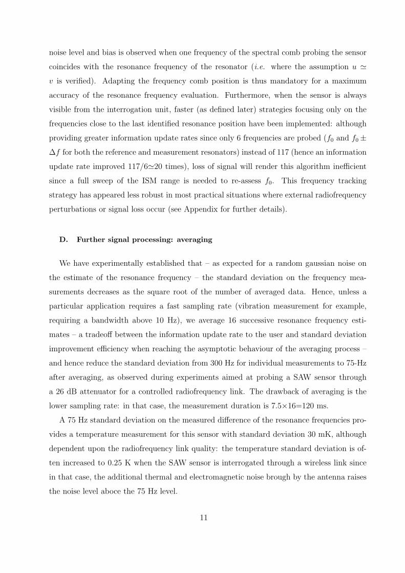
D. Further signal processing: averaging

We have experimentally established that – as expected for a random gaussian noise on

the estimate of the resonance frequency – the standard deviation on the frequency mea-

surements decreases as the square root of the number of averaged data. Hence, unless a

particular application requires a fast sampling rate (vibration measurement for example,

requiring a bandwidth above 10 Hz), we average 16 successive resonance frequency esti-

mates – a tradeoff between the information update rate to the user and standard deviation

improvement efficiency when reaching the asymptotic behaviour of the averaging process –

and hence reduce the standard deviation from 300 Hz for individual measurements to 75-Hz

after averaging, as observed during experiments aimed at probing a SAW sensor through

a 26 dB attenuator for a controlled radiofrequency link. The drawback of averaging is the

lower sampling rate: in that case, the measurement duration is 7.5×16=120 ms.

A 75 Hz standard deviation on the measured difference of the resonance frequencies pro-

vides a temperature measurement for this sensor with standard deviation 30 mK, although

dependent upon the radiofrequency link quality: the temperature standard deviation is of-

ten increased to 0.25 K when the SAW sensor is interrogated through a wireless link since

in that case, the additional thermal and electromagnetic noise brough by the antenna raises

the noise level aboce the 75 Hz level.

11

VI. RESULTS AND APPLICATIONS EXAMPLES

We assess experimentally the strategy described so far by interrogating a SAW sensor

designed for the measurement of temperature. The TCF of this dual resonator sensor is

2500 Hz/K (6 ppm/K) as defined earlier (see section II). The two aims of these measurements

are

• the estimation on a static sensor of the resolution of the measurement, i.e. the assess-

ment of the various causes of noise and bias on the resonance frequency measurements

as the sensor is constantly seen by the interrogation unit

• the estimation of the minimum duration during which a sensor must be visible from

the interrogation unit to perform a measurement, and hence the maximum speed at

which a mobile object supporting the sensor might move with respect to the static

interrogation electronics. In that case, we assume that the sensor is periodically visible

from the interrogation unit in order to perform successive averages even though the

sensor is not constantly accessible via the RF link(as is the case on a rotating object

such as a motor axis or a wheel).

The current implementation of the strategies described so far has been implemented with

sampling the ISM frequency range with 128 points (more than the required 117 points for

digital computation efficiency), with frequency steps of 13.3 kHz. The emission duration is

selected so that the corresponding power spectrum is narrower than the resonator resonance:

with an experimental Q at 434 MHz around 10000, we select an emission duration of 30 µs.

The signal processing duration and DDS programming step require another 30 µs, for a

total ISM sweep 7.5 ms long. As explained previously, we perform 16 averages to reduce the

frequency detection standard deviation below 200 Hz, so the physical quantity measurement

is updated every 120 ms. The samples of the average do not need to be contiguous: we

accumulate samples until either the wanted number of samples is reached, or a timeout is

reached. The resulting algorithm is stable even with sensors only intermittently visible to

the interrogation antenna. The requirement is that the sensor is seen by the interrogation

antenna at least 7.5 ms: this condition is met on a 30 cm radius wheel rotating at 37 Hz

(2600 rpm or 300 km/h driving speed) when the visibility angle is 120o. The antenna hence

is of utmost importance when interrogating sensors located on a rotating object: the greater

12

the angular coverage of the interrogation and sensor antennas, the higher the speed at which

the rotating sensor will be usable.

The influence of the number of sampled frequencies within the ISM band on the measure-

ment accuracy is experimentally assessed as illustrated in Fig. 6. Although a small number

of sampled frequencies is suitable to increase the measurement rate (and hence reduce the

needed visibility duration of the sensor, or increase the motion velocity of the sensor with

respect to the fixed interrogation antenna), too small a number n (n 1.7 MHz 3Qf0

) yields

a bias on the measurement associated with the non-parabolic shape of the resonance. This

bias is experimentally observed and defines the minimum number of sampled frequencies:

we typically sample 128 frequencies within the 434-MHz ISM band (13,3 kHz steps).

VII. CONCLUSION

We have demonstrated the use of a versatile system for the wireless interrogation of pas-

sive surface acoustic wave sensors in the 434-MHz frequency range inspired from RADAR

techniques. A full software control of all interrogation steps – from the emitted signal fre-

quency to duplexer switching between emission and reception stages and RF power magni-

tude sampling – provides the means to implement various strategies for probing the resonant

frequency of resonating sensors. Signal processing strategies such as the interrogation scheme

presented here reduce the number of sampled frequencies so that the interrogation steps are

compatible with a sensor visible by the interrogation unit for less than 10 ms, as is typically

seen on rotating objects such as wheels or rotating axis in industrial applications. These

signal processing steps, if not properly modeled and understood, might yield unwanted mea-

surement artifacts as was demonstrated theoretically and experimentally. Finally, it turns

out that a simple versatile interrogation electronics reveals particulary adapted for testing

various strategies and RF link protocols able to improve wireless sensing system features.

Different approaches will be further tested in that matter.

13

Acknowledgments

The authors acknowledge fruitful discussions with L. Fagot-Revurat (MFPM, France).

∗ Electronic address: jmfriedt@femto-st.fr

1 T. Liu, C. Sadler, P. Zhang, and M. Martonosi, in MobiSYS’04 (2004).

2 L. Krishnamurthy, R. Adler, P. Buonadonna, J. Chhabra, M. Flanigan, N. Kushalnagar,

L. Nachman, and M. Yarvis, in 3rd international conference on embedded networked sensor

systems (2005), pp. 64–75.

3 X. Conghui, G. Peijun, C. Wenyi, T. Xi, Y. Na, and M. Hao, Journal of Semiconductors 30,

045003 (2009).

4 N. Cho, S.-J. Song, S. Kim, S. Kim, and H.-J. Yoo, in Proc. of the 31st Solid-State Circuits

Conference (2005), pp. 279–282.

5 P. Pursula, J. Marjonen, H. Ronkainen, and K. Jaakkola, in Transducers & Eurosensors’07

(2007), pp. 73–76.

6 T. Nomura, A. Saitoh, and H. Tokuyama, in WCU (2003), pp. 935–938.

7 Y. Dong, W. Cheng, S. Wang, Y. Li, and G. Feng, Sensors and Actuators B 76, 130 (2001).

8 G. Scholl, F. Schmidt, T. Ostertag, L. Reindl, H. Scherr, and U. Wolff, in IEEE International

frequency control symposium (1998), pp. 595–601.

9 A. Springer, R. Weigel, A. Pohl, and F. Seifert, Mechatronics 9, 745 (1999).

10 F. Schmidt, O. Sczesny, L. Reindl, and V. Mhgori, in IEEE Ultrasonics Symposium (1994), pp.

589–592.

11 G. Bruckner, R. Hauser, A. Stelzer, L. Maurer, L. Reindl, R. Teichmann, and J. Biniasch, in

Proceedings of the 2003 IEEE International Frequency Control Symposium and PDA Exhibition,

Jointly with the 17th European Frequency and Time Forum (2003), pp. 942–947.

12 W. Bulst, G. Fischerauer, and L. Reindl, IEEE Transactions on Industrial Electronics 48, 265

(2001).

13 L. Reindl and I. Shrena, IEEE transactions on utrasonics, ferroelectrics, and frequency control

51, 1457 (2004).

14 S. Schuster, S. Scheiblhofer, L. Reindl, and A. Stelzer, IEEE transactions on utrasonics, ferro-

14

electrics, and frequency control 53, 1177 (2006).

15 H. Scherr, G. Scholl, F. Seifert, and R. Weige, in IEEE Ultrasonics Symposium (1996), pp.

347–350.

16 A. Pohl, G. Ostermayer, L. Reindl, and F. Seifert, in IEEE Ultrasonics Symposium (1997).

17 A. Pohl and L. Reindl, in Advanced Microsystems for Automotive Applications Conference

(1998), pp. 250–262.

18 H. Oh, W. Wang, K. Lee, I. Park, and S. Yang, International journal on smart sensing and

intelligent systems 1, 940 (2008).

19 A. Pohl, R. Steindl, and L. Reindl, IEEE transactions on instrumentation and measurement

48, 1041 (1999).

20 J. Beckley, V. Kalinin, M. Lee, and K. Voliansky, in IEEE International Frequency Control

Symposium and PDA Exhibition (2002), pp. 202–213.

21 M. Dierkes and U. Hilleringmann, Advances in Radio Science 1, 131 (2003).

22 A. Stelzer, G. Schimetta, L. Reindl, A. Springer, and R. Weigel, in SPIE Proceedings – Subsur-

face ans Surface Sensing Technologies and Applications III (2001), vol. 4491, pp. 358–366.

23 J. H. Kuypers, M. Esashi, D. A. Eisele, and L. M. Reindl, in IEEE Ultrasonics Symposium

(2006), pp. 1453–1458.

24 R. White and F. Voltmer, Applied Physics Letters 7, 314 (1965).

25 A.Pohll, F.Seifert, L.Reind, G.Scholl, T. Ostertag, and W.Pietschl, in IEEE Ultrasonics Sym-

posium (1994), pp. 195–198.

26 L. Reindl, G. Scholl, T. Ostertag, C. Ruppel, W.-E. Bulst, and F. Seifert, in IEEE Ultrasonics

Symposium (1996), pp. 363–367.

27 R. Brocato, Sandia Report pp. 1–20 (2006).

28 L. Reindl, 2nd Int. Symp. Acoustic Wave Devices for Future Mobile Communication Systems

pp. 1–15 (2004).

29 X. Q. Bao, W. B. an V.V. Varadan, and V. Varadan, in IEEE Ultrasonics Symposium (1987),

pp. 583–585.

30 C. Hartmann, in Proceedings of 2002 IEEE Ultrasonics Symposium (2002).

31 C. S. Hartmann, P. Brown, , and J. Bellamy, in Proceedings of the Second International Sym-

posium on Acoustic Wave Devices for Future Mobile Communication Systems (2004).

32 P. Hartmann, in IEEE International Conference on RFID (2009), pp. 291–297.

15

33 W. Buff, F. Plath, . Schmeckebier, M. Rusko, T. Vandahl, H. Luck, F. Moller, and D. Malocha,

in IEEE Ultrasonics Symposium (1994), pp. 585–588.

34 T. Osterag and S. Kunzmann, IQ-mobil Gmbh pp. 1–9 (2003).

35 A. Pohl, G. Ostermayer, and F. Seifert, IEEE transactions on ultrasonics, ferroelectrics, and

frequency control 45, 1061 (1998).

36 Y. Wen, P. Li, J. Yang, and M. Zheng, IEEE sensors journal 4 (2004).

37 A. Stelzer, R. Hauser, L. Reindl, and R. Teichmann, in XVII IMEKO World Congress (2003),

pp. 672–675.

38 S. Segars, K. Clarke, and L. Gourdge, IEEE Micro pp. 22–30 (1995).

39 R. Matsuzakia and A. Todoroki, Sensors and Actuators A 119, 323 (2005).

40 W. Buff, S. Klett, M. Rusko, J. Ehrenpfordt, and M. Goroli, IEEE transactions on ultrasonics,

ferroelectrics, and frequency control 45, 1388 (1998).

41 W. Buff, M. Rusko, M. Goroll, J. Ehrenpfordt, and T. Vandahl, in IEEE Ultrasonics Symposium

(1997), pp. 359–362.

42 A. Stelzer, S. Schuster, and S. Scheiblhofer, in International Workshop on SiP/SoC Integration

of MEMS and Passive Components with RF-ICs (2004).

43 F. Cordara and V. Pettiti, in Proceedings of the 27th Precise Time and Time Interval (PTTI)

Applications and Planning Meeting (1995), pp. 113–124.

44 W. Lewandowski, P. Moussay, P. Guerin, F. Meyer, and M. Vincent, in 11th European and

Time Forum (EFTF) (1997), pp. 493–497.

45 K. Kalliomaki, T. Mansten, and A. Rautiainen, in Joint IEEE International Frequency Control

Symposium with the 21st European Frequency and Time Forum (2007), pp. 865–867.

46 G. Martin, P. Berthelot, J. Masson, W. Daniau, V. Blondeau-Patissier, B. Guichardaz, S. Bal-

landras, and A. Lamber, in IEEE Ultrasonics Symposium (2005), vol. 4, pp. 2089–2092.

47 in Maxim Application Note 127 (2001).

48 D. Dye, Proc. Phys. Soc. London 38, 399 (1925).

49 K. V. Dyke, Phys. Rev. 25, 895 (1925).

16

Appendix

One aspect associated with digital signal processing and the bias induced by the parabolic

fit of the received signals is to identify the origin of the bias and whether a better processing

technique might remove it.

Here we are modelling the parabolic fit on noisy data generated from a three points

along a parabola y = −x2 (x = x0;x0 + 1;x0 + 2 and x0 ∈ [−1.5 : −0.5]) to which a

uniformly distributed noise in the [−0.5 : 0.5] range is added. We then plot the position of

the estimated parabola maximum as a function of two processing algorithms:

1. first fitting the noisy data with a parabolic fit, identifying the position of the maximum

of this fitted parabola, and after accumulating 16 estimates, averaging the estimates

to deduce the resonance position

2. averaging multiple (16) noisy measurements for averaging, and performing a single

parabolic fit on the averaged data

Not only is the second strategy more efficient in terms of computational power (only

one multiplication is needed instead of the 16 multiplications for each iteration of the first

algorithm), but Fig. 7 shows that the standard deviation on 1500 simulations is lower or

equal for the second algorithm compared to the first one, but most significantly that the

bias is strongly reduced by first averaging the raw measurements followed by the parabolic

fit instead of averaging the results of the fits.

One interesting aspect of Fig. 7 is that the bias of the estimated resonance frequency

to the true frequency is not associated with the approximation due ti the second order

Taylor development of the resonance shape but is intrinsic to fitting noisy measurements

along the parabola and averaging multiple maxima position estimates. This theoretical

result is confirmed by experimental measurements 8: in this experiment, a dual resonator

is connected throught a 23 dB attenuator to the RF output of the interrogation unit. The

resonance frequency of both resonance and measurement modes are monitored using either

an averaging (16 values) of each resonance position estimated following a polynomial fit

(i.e. average of the frequency position), or a single parabolic on the average of the returned

signals.

The first algorithm is nevertheless used for mobile sensor probing since each measurement

17

is individually validated for incorporation in the average following a threshold criterion: this

identification of the presence of the sensor in view of the interrogation unit is not possible

when all ISM frequency sweep results are accumulated for later parabolic fitting analysis.

Figures

amplification

and band−pass

filtering

switchesfrequency

synthesis

duplexer

amplification

and band−pass

filtering

power

detector

low frequency

amplification

+ offset

removal

antenna

A/D conversion

sampling

ARM7 CPU

frequency

programming

analog &

digital outputs

FIG. 1: General strategy of the narrowband wireless acoustic sensor interrogation unit.

-120

-110

-100

-90

-80

-70

-60

10 100 1000 10000 100000 1000000

phas

e no

ise

(dB

c/H

z)

frequency offset (Hz)

mixer 400+35 MHzDDS only 435 MHz

clockfrequency fckfrequency f

output

f+fck

f−fck

(a) (b)

(a) (b)

18

FIG. 2: (a) Comparison of the phase noises of 435 MHz signals obtained by mixing a 400 MHz

signal resulting of a PLL multiplication of a 20 MHz source and a 35 MHz output of a DDS

clocked by this same 20 MHz source internally multiplied to 400 MHz ; and by the band-pass

filtered 435 MHz output of this same DDS resulting from the intrinsic generation of a signal at

a frequency which is the sum of the clock and output signal frequencies. (b) Raw output of the

AD9954 DDS clocked at fck = 400 MHz and programmed to output a frequency f = 33 MHz.

The 400+33 MHz output is bandpass filtered using two SAW filters and amplified to 0 dBm for

generating the radiofrequency probe pulse.

(f0, s0)

(f3, s3)(f2, s2)

(f1, s1)

∆ffrequency (a.u.)

∆f

u

v

rece

ived

sign

alst

rengt

h(a

.u.)

FIG. 3: Three measurements of the received signal magnitude s1, s2 and s3 at three probe fre-

quencies f1, f2 and f3 respectively are fitted using a second order polynom in order to identify the

true resonance frequency f0.

19

0.0050.01

0.0150.02

0.0250.03

0.0350.04

0.0450.05

433.55 433.6 433.65 433.7 433.75 433.8

Y11

(m

hos)

frequency (MHz)

BvD model (Q=10000)parabolic fit

-0.5

0

0.5

1

1.5

433.66 433.665 433.67 433.675 433.68 433.685 433.69

para

bolic

app

roxi

mat

ion

erro

r (%

)

frequency (MHz)

FIG. 4: Top: comparison of a BvD model (L1 = 72.8 µH, C1 = 1.85 fF, R1 = 21 Ω, C0 = 3.3 pF)

and the parabolic fit around resonance f0, in the frequency domain in the range f0 ±∆f0/(3Q).

Bottom: zoom on this same frequency region, with the display of the error between the model and

the parabolic approximation in %.

100200300400500600700800900

1000

-15000 -10000 -5000 0 5000 10000 15000

Fre

quen

cy e

stim

ate

stan

dard

dev

iatio

n (H

z)

Frequency comb offset (Hz)

16 averages

SNR=5SNR=15SNR=25SNR=50

-800-600-400-200

0200400600800

-15000 -10000 -5000 0 5000 10000 15000Fre

q. e

stim

ate

offs

et (

Hz)

Frequency comb offset (Hz)

16 average

SNR=5SNR=15SNR=25SNR=50

20

FIG. 5: Monte Carlo simulations of noisy reflected signal magnitude following a Butterworth van

Dyke model (L1=72.8 µH, C1=1.85 fF, R1=21 Ω and C0=3.3 pF yielding a theoretical resonance

frequency of 433674982 Hz and a quality factor around 9500, consistent with available sensor

characteristics. With these values, ∆f = 15.3 kHz. The standard deviation and bias of the

estimated frequency f0 to the true resonance frequency are maximum when the resonance frequency

is in the middle of two frequencies of the comb, and are minimum when one frequency of the

comb matches the resonance frequency. In this simulation, the frequency comb was centered on

433679185 Hz, i.e. an offset of 4202 Hz to the true resonance frequency of the device.

250000

300000

350000

400000

450000

500000

0 500 1000 1500 2000 2500

freq

uenc

y di

ffere

nce

[Hz]

time [a.u.]

48 points64 points

128 points

-15000

-10000

-5000

0

5000

10000

15000

0 500 1000 1500 2000 2500b

ias(6

4 v

.s 1

28

) [H

z]

time [a.u.]

-15000

-10000

-5000

0

5000

10000

15000

20000

0 500 1000 1500 2000 2500

bia

s(4

8 v

.s 1

28

) [H

z]

time [a.u.]

300

450

(a) (b)

FIG. 6: Bias on the estimated resonance frequency difference experimentally observed during a

sensor heating and cooling experiment (top): the ISM band was scanned with 48, 64 and 128 steps.

Although the general trend and the average value are independent of the number of sampled

frequencies in the ISM band, the bias associated with the parabolic shape are clearly observed, and

magnified on the bottom curve by subtracting the curve with highest sampling rate (128, assumed

to be representative of the actual heating and cooling kinetic) from the two other curves (64 and

48 sampled frequencies). Note that the distance between the first two bias maxima are separated

by a distance scaling with the number of sampled frequencies : 450/300=64/48, in agreement with

our interpretation of the origin of the bias associated with the spacing between the frequencies of

the comb.

21

0.06

0.05

0.04

0.03

0.5st

anda

rd d

ev0

offset

-0.5

16 averages, 1500 experiments

0.05

0

-0.05

0.50-0.5

offset

bias

FIG. 7: Standard deviation and bias of the estimated parabola maximum as a function of the

position of f1, f2 and f3 with respect to the true maximum f0 = 0. Here ∆f = 1.

4.3369e+08

4.337e+08

4.3371e+08

4.3372e+08

4.3373e+08

4.3374e+08

4.3375e+08

4.3376e+08

0 200 400 600 800 1000 1200 1400 1600

tem

pera

ture

dep

ende

nt m

ode

reso

nant

freq

uenc

y (H

z)

time (a.u.)

0

100

200

300

400

500

0 10000 20000 30000 40000 50000 60000 70000

freq

. sta

ndar

d de

viat

ion

[Hz]

resonance frequency shift and frequency comb position (Hz)

-1000

-500

0

500

1000

0 10000 20000 30000 40000 50000 60000 70000

fit o

f ave

rage

s -

aver

age

of fi

ts (

Hz)

resonance frequency shift and frequency comb position (Hz)

(a) (b)

22

FIG. 8: (a) Time evolution of a temperature sensitive resonance as the sensor is heated by a

2 A current running through a 1 Ω resistor. (b) Top: experimental measurement of the difference

between the resonance position maximum estimated by averaging 16 parabola maxima measured on

noisy data on the one hand, and estimating from a single parabola fit on 16 measurement averages

on the second hand. The red lines are spaced by a frequency comb spacing (∆f = 17.74 kHz in this

example) and show that indeed the maximum noise level is observed with such a periodicity. (b)

Bottom: experimental measurement of the standard deviation of the 16 frequencies accumulated

for computing each sample in the parabola maxima averaging strategy. The red lines are spaced by

a frequency comb spacing (∆f = 17.74 kHz in this example) and show that indeed the maximum

noise level is observed with such a periodicity.

23