Embed Size (px)
Citation preview
A Vector Error Correction Almost Ideal Demand Model for Organic Milk in the USA
Ye Su
University of Missouri
324 Mumford Hall
Columbia, MO 65211
Michael L. Cook
University of Missouri
125C Mumford Hall
Selected Paper prepared for presentation at the 2015 Agricultural & Applied
Economics Association and Western Agricultural Economics Association Annual
Meeting, San Francisco, CA, July 26-28
Copyright 2015 by Ye Su, and Michael L. Cook. All rights reserved. Readers may make
verbatim copies of this document for noncommercial purposes by any means, provided
that this copyright notice appears on all such copies.
1
Abstract
The objective of this study is to develop an econometric model for the demand analysis of
organic and conventional milk in the USA by applying time series techniques. The results
of the study can shed lights for policy making, marketing and production of organic and
conventional dairy sections. The monthly aggregate organic and conventional fluid milk
data from 2006 to 2013 are used for the analysis. A vector error correction almost ideal
demand model with habit persistence is adopted to model the short and long run effects of
consumer demand for milk. Price and expenditure endogeneity are also explored by
introducing instrumental variables. The results show that the time series data are non-
stationary at the level, but stationary at the first difference. The budget share, price and
expenditure are cointegrated and the error correction terms are significant in the dynamic
model. The prices are exogenous, but the group expenditure is endogenous. Therefore, the
dynamic model with cointegration framework is a better model for the demand analysis.
The price and expenditure elasticities estimated from three different models are compared
and contrasted. The results show organic milk is more price elastic than conventional milk,
but is still price inelastic. Organic milk is expenditure elastic, but the conventional milk is
expenditure inelastic.
2
1 Introduction
The total organic food sales were $35.9 billion in 2014, up 11% from 2013 (Organic
Trade Association 2015). The organic dairy sales were $5.46 billion in 2014 and 15.2% of
the organic food sales, and also had 11% growth from previous year. The organic dairy is
the second largest group after organic fruits and vegetables. Compared with conventional
fluid milk, organic fluid milk sales have grown at a rate of more than 10% per year since
2006 vs. flat or declining conventional milk sales1. There is little published work on organic
milk demand and factors affecting the demand in the U.S. Current available studies use
household survey or retail scanner data, which exclude away from home and school
consumption. The household data representing one year cannot provide time varying
variables such as income and consumer preference and taste. A few articles used retail
scanner time-series data, but no studies considered time series properties (Chang et al. 2011,
Li, Peterson, and Tian 2012).
The majority of studies in the U.S. about organic milk demand model use Neilsen
homescan data. Two of them use the 2004 data (Alviola and Capps 2010, Chikasada 2008).
The USDA National Organic Program was enforced in October 2002. As of 2004, organic
milk consumers were still relatively new to the new labeling and regulation. Two national
organic milk brands totaled 80% of the market share in 2004 (Dimitri and Venezia 2007).
Since then, private label organic milk sales have been increasing dramatically2. More than
100 local, regional, and store brands of organic milk have emerged3. Organic food is now
1 Calculated with AMS-USDA, Federal Milk Market Order statistics, www.ams.usda.gov. 2 http://www.nodpa.com/payprice_update_02062013.shtml 3 Organic Dairy Report - Cornucopia Institute,
http://www.cornucopia.org/dairysurvey/Ratings_Alphabetical.html
3
sold in almost all of the traditional venues. The variety of organic milk also has increased.
Flavored organic milk and DHA fortified organic milk are two examples. The market for
organic milk is maturing. Consumers’ preference and taste change along with the organic
milk market. These factors can have profound effects on consumer purchasing behavior.
The most recent data of organic milk demand studies are from 2010 (Li, Peterson, and Tian
2012). Therefore, it is necessary to provide an update on the status of consumer demand
for organic milk. This study is aimed to fill this gap.
Three studies (Chang et al. 2011, Glaser and Thompson 2000, Li, Peterson, and Tian
2012) have used time series data to consider habit formation, but they have not considered
time series properties and possible non-stationary property of the data. Although the
ordinary least square (OLS) estimator of time series data is consistent, the inference of the
estimation will be invalid if the data are not cointegrated. This is because the OLS
technique requires that the error term are variance covariance stationary and
autocovariance are finite and constant over time. Non-stationary time series data do not
meet the requirements for OLS regression. Cointegration provides a framework for non-
stationary time series data, which is explored in this study.
The objective of this study is to consider both long-run and short-run relationship
among consumer demand, price, and expenditure and provide information for organic and
conventional milk demand in the USA by using time series techniques. The article is
organized as follows: section 2 and 3 introduce the almost ideal demand system (AIDS)
and vector error correction (VEC) AIDS, section 4, 5, and 6 give introduction about the
data, endogeneity of price and income, section 7 and 8 present time series analyses, section
4
9 provides the analysis of organic and conventional milk demand results, and the last
section summarizes and concludes the paper.
2 Almost Ideal Demand System
Even though there are many demand models available, AIDS (Deaton and
Muellbauer 1980) is the most popular one since it was published because it satisfies all the
requirements of consumer theory. AIDS starts from a first order approximation of a cost
function and derived through utility maximization. A few assumptions are made in the
model: prices and income are exogenous, and the interested goods are weakly separable
from other goods. Two-stage budget process is also assumed. In the first stage, the
expenditure is assigned to different groups of goods. In the second stage, the expenditure
is allocated within each group. The primary concern of this study focuses on the second
stage. The AIDS is defined as follow:
𝑤𝑖𝑡 = 𝑎𝑖 + ∑ 𝑟𝑖𝑗𝑙𝑜𝑔𝑝𝑗𝑡 + 𝛽𝑖 log (𝑥𝑡
𝑃𝑡) + 휀𝑖𝑡
𝑛
𝑗=1
𝑖, 𝑗 = 1 𝑡𝑜 𝑛 represent the number of interested goods in the model and equals three in this
paper. Where 𝑤𝑖𝑡 is the budget share of subcategory i in total milk expenditure at time t, 𝑎𝑖
is intercept, pjt is the price of j subcategory at time t. 𝑥𝑡 is the total expenditure on the
interested goods, 𝑃𝑡 is a translog price index, and 𝑥𝑡
𝑃𝑡 is considered as the real expenditure.
𝛽𝑖 reflects the effect of real expenditure on budget share holding the price constant. Positive
𝛽𝑖 means luxury goods and negative means necessary goods. The price index 𝑃𝑡 is defined
by the following formula and is nonlinear:
5
𝑙𝑜𝑔𝑃𝑡 = ∑ 𝑙𝑜𝑔𝑃𝑖𝑡 + 0.5 ∑ ∑ 𝑟𝑖𝑗
𝑗𝑖
log 𝑃𝑖𝑡𝑙𝑜𝑔𝑃𝑗𝑡
𝑛
𝑖=1
The nonlinear price index is difficult to estimate in empirical study. Deaton and Muellbauer
proposed a linear approximate of the price index by using Stone Price index and is known
as linear AIDS (LAIDS), where
𝑙𝑜𝑔𝑃𝑡∗ = ∑ 𝑤𝑖𝑡𝑙𝑜𝑔𝑃𝑖𝑡
𝑛
𝑖=1
In order to meet the choice theory, a few constraints need to be met. The adding up
conditions are automatically satisfied if:
∑ 𝑎𝑖 = 1,𝑖 ∑ 𝑟𝑖𝑗 = ∑ 𝛽𝑖 = 0𝑖𝑖
Homogeneity and symmetry conditions are imposed by satisfying the following constrains:
∑ 𝑟𝑖𝑗 = 0 𝑎𝑛𝑑 𝑟𝑖𝑗 = 𝑟𝑗𝑖 , ∀𝑖, 𝑗 𝑖 ≠ 𝑗
𝑗
In practice, one of the equations is dropped in the estimation to meet the adding up
constraint. This makes the homogeneity and adding up condition automatically met.
Uncompensated price elasticity for LAIDS is calculated by the formula:
휀𝑖𝑗𝑀 = −𝛿𝑖𝑗 +
𝑟𝑖𝑗
𝑤𝑖− 𝛽𝑖
𝑤𝑗
𝑤𝑖,
𝛿𝑖𝑗 is the Kronecker delta =1 for i=j and = 0 otherwise. 𝑤𝑖 is the mean expenditure share
across the sample for good i. Compensated price elasticity formula is:
휀𝑖𝑗𝐻 = 휀𝑖𝑗
𝑀+𝛽𝑖𝑤𝑗 = = −𝛿𝑖𝑗 +𝑟𝑖𝑗
𝑤𝑖+ 𝑤𝑗
Expenditure elasticity is calculated by this formula: 𝜂𝑖 = 1 + (𝛽𝑖
𝑤𝑖)
6
3 Vector Error Correction (VEC) AIDS
The original AIDS model assumes that the error terms are uncorrelated and
normally distributed. This assumption can be a problem in time series data because of the
non-stationarity of the series, i.e., the covariance of a series changes over time. In fact,
many time series data are first difference covariance stationary instead of level stationary.
The first difference covariance stationary series is called integrated at order one, I(1)
process. One popular method to regress non-stationary data is to use the first difference.
However, if the time series are cointegrated, the simply first difference will misspecify the
model. Two variables are cointegrated if each is an I(1) process but a linear combination
of them is an I(0) process. For example:
𝑦𝑡 = 𝑎 + 𝑥𝑡 + 𝜇𝑡, 𝑦𝑡 𝑎𝑛𝑑 𝑥𝑡 𝑎𝑟𝑒 I(1) processes
𝜇𝑡 = 𝑦𝑡 − 𝑎 − 𝑥𝑡, if 𝜇𝑡 is a I(0) process, 𝑦𝑡 𝑎𝑛𝑑 𝑥𝑡 are cointegrated.
In addition, the regular AIDS model only considers the static aspect or long run
relationship of the demand system. Vector Error Correction model (VECM) adds short run
dynamic aspect to the long run equilibrium relationship. By including an error correction
term in the model, VECM incorporates the mechanism of short run adjustment of
consumption to move the short run disequilibrium back to the long run equilibrium. This
model includes unit root test, cointegration test and then VECM modelling. There are a
number of unit root test methods available. Augmented Dickey Fuller test (ADF) is used
in this study. The estimated regression of ADF is specified as:
∆𝑌𝑡 = 𝛼 + 𝛿𝑡 + 𝜌𝑌𝑡−1 + ∑ 𝜑𝑖∆𝑌𝑡−𝑖 + 𝑢𝑖
𝑝
𝑖=1

7
𝑌𝑡 is a random variable with no zero mean, 𝛼 is constant, t is a time trend, and µ is
the error term with iid (0, 𝜎2) distribution. The null hypothesis is that the time series is
non-stationary and 𝜌 = 1. The alternative hypothesis is the time series is stationary. Under
the null hypothesis, the test statistics has Dickey Fuller distribution. Non-stationary time
series is differenced until they are stationary and the degree of integration is determined by
the times of difference.
If the time series are integrated at the same degree, Johansens’ maximum likelihood
cointegration test is used to test the cointegration of the series. The cointegration represents
the long term relationship among price, expenditure and budget share of the demand model.
The null hypothesis is that the series are not cointegrated.
Traditional almost ideal demand system uses simultaneous price and expenditure
data with budget share. This is considered as long term effects. In the long run, there is an
equilibrium among price, expenditure and budget share. In the short run, due to asymmetric
information, transaction costs, consumption pattern, and preference consistent, there is a
period of adjustment of consumption to the price and income change, or there is a delay of
adjustment to price and income change. The delay of adjustment makes the consumption
deviate from the long run equilibrium. This is called short-run disequilibrium. The static
model does not include the dynamic adjustment in the specification. The dynamic model
solves this problem by including the short-run adjustment in the model using the vector
error correction model (VECM). A vector error correction model is specified as:
∆𝑌𝑡 = 𝑐 + 𝛼′𝛽(𝑌𝑡−1) + ∑ ∅𝑗 ∆𝑌𝑡−𝑗
𝑗
+ 휀𝑡
8
𝛽 is the cointegrating vector, c is constant, α and ∅ are coefficients. 휀𝑡 is the error
term with identical and independent distribution. 𝛽(𝑌𝑡−1) is the error correction term and
is estimated by the lagged residual of the OLS regression of the static demand equations.
Due to the nonlinear property of AIDS, LAIDS is used in the VECM model. The VEC
LAIDS is defined as:
∆𝑤𝑖 = 𝛼 + 𝛿′𝜗(𝑤𝑖𝑡−1) + ∑ 𝑟𝑖𝑗 ∆𝑙𝑛𝑝𝑗
𝑖
+ 𝛽𝑖∆ log (𝑥
𝑃∗) + 휀𝑖
Or
∆𝑤𝑖 = 𝛼 + 𝜃∆𝑤𝑖𝑡−𝑘 + 𝛿′(𝜇𝑖𝑡−1) + ∑ 𝑟𝑖𝑗 ∆𝑙𝑛𝑝𝑗
𝑖
+ 𝛽𝑖∆ log (𝑥
𝑃∗) + 휀𝑖
Lagged budget share is included in the dynamic equation to reflect the persistence
of consumption habit and the delay of consumer response to the price and income change.
The error correction term 𝜇𝑖𝑡−1 is a disequilibrium error from the long run equilibrium. The
coefficient of the error correction term is expected to be negative and reflects the
adjustment to return back to the long run relationship. The lower the coefficient, the slower
the correction goes back to the long run equilibrium and the stronger is the habit effect. 𝜃
and 𝛿 represent short run dynamic of the demand system. The model is estimated using an
iterated seemingly unrelated regression procedure in Stata version 13.
4 Data
This study focuses on organic and conventional fluid milk consumption in the U.S.,
because the majority of organic milk is consumed as fluid milk (about 70%). The data used
in this study is aggregate monthly sales and price for organic milk as a whole and
conventional whole and reduced fat milk (2%, 1%, and skim) over the period 2006-2013.
9
The reason for combining the organic milk as a whole is the prices of organic whole and
organic reduced fat milk are almost the same in the studied period. The choice of milk is
not affected by the price, but by the consumer preference. Totally there are 96 observations.
The data are available from Agricultural Marketing Service (AMS) of the USDA. The
monthly U.S. population data are downloaded from the U.S. Census Bureau. The per capita
consumption data are calculated by the total sales divided by population. The prices are
average across the U.S. The expenditure on each type of milk is calculated by the retail
price multiplied by quantity consumed. The budget share is calculated by the expenditure
on each goods divided by the total expenditure on all milk. The descriptive statistics of the
data are provided in Table 1.
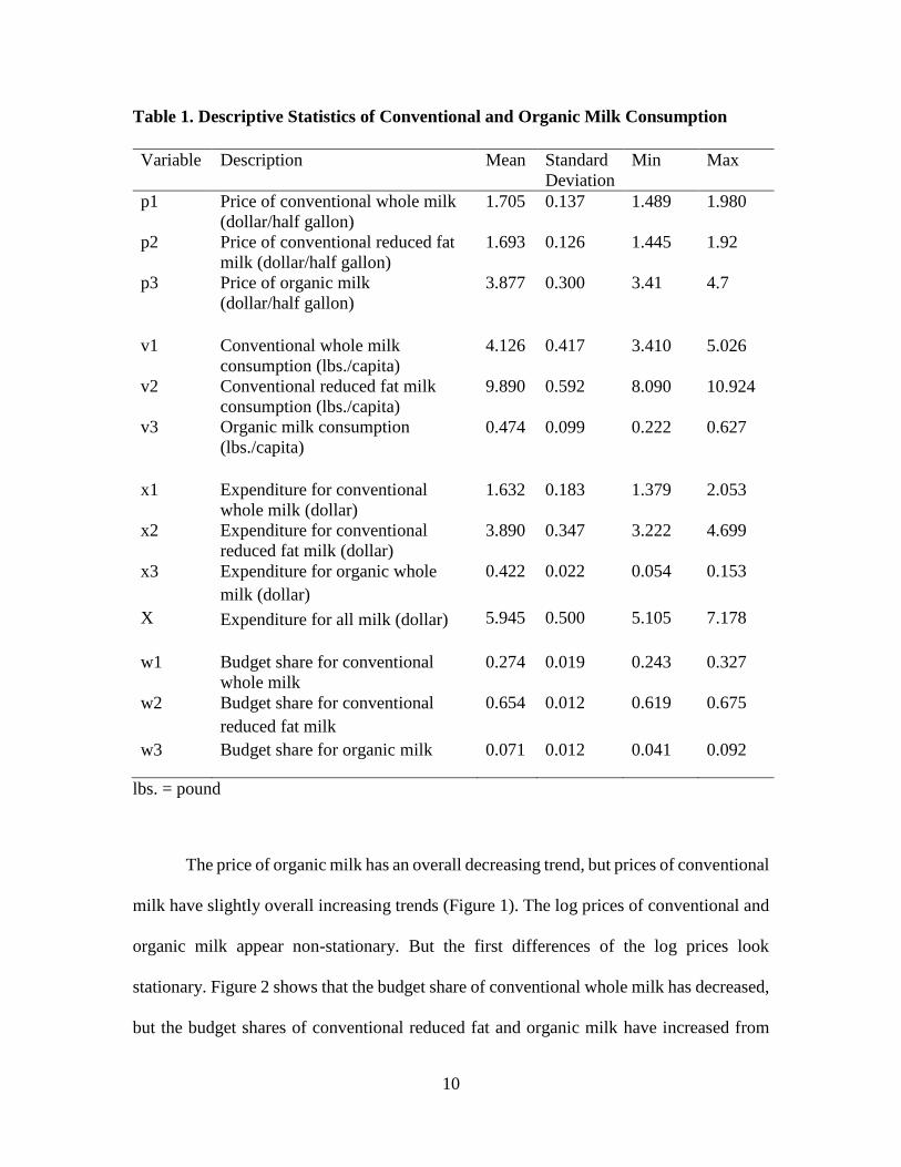
The descriptive statistics (Table 1) indicate that the price of organic milk is more
than two times of the conventional milk in the studied period. The prices of conventional
whole and reduced fat milk are close to each other (1.705, 1.693/half gallon). The
consumption of organic milk is very low, only 3.3% of total fluid milk. The consumption
of reduced fat conventional milk is the highest and is up to 68% of total milk consumption.
Regarding to the budget share, organic milk is about 7% of total expenditure, while the
conventional milk accounts for the rest 93%. The average total monthly milk consumption
is 14 pounds (1.68 gallon; one gallon milk is equal to 8.6 pounds) per capita, which cost
about six dollars on average.
10
Table 1. Descriptive Statistics of Conventional and Organic Milk Consumption
lbs. = pound
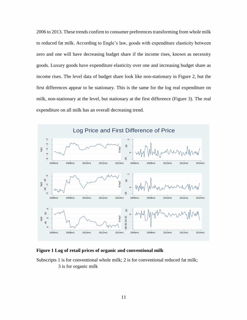
The price of organic milk has an overall decreasing trend, but prices of conventional
milk have slightly overall increasing trends (Figure 1). The log prices of conventional and
organic milk appear non-stationary. But the first differences of the log prices look
stationary. Figure 2 shows that the budget share of conventional whole milk has decreased,
but the budget shares of conventional reduced fat and organic milk have increased from
Variable Description Mean Standard
Deviation
Min Max
p1 Price of conventional whole milk
(dollar/half gallon)
1.705 0.137 1.489 1.980
p2 Price of conventional reduced fat
milk (dollar/half gallon)
1.693 0.126 1.445 1.92
p3 Price of organic milk
(dollar/half gallon)
3.877 0.300 3.41 4.7
v1 Conventional whole milk
consumption (lbs./capita)
4.126 0.417 3.410 5.026
v2 Conventional reduced fat milk
consumption (lbs./capita)
9.890 0.592 8.090 10.924
v3 Organic milk consumption
(lbs./capita)
0.474 0.099 0.222 0.627
x1 Expenditure for conventional
whole milk (dollar)
1.632 0.183 1.379 2.053
x2 Expenditure for conventional
reduced fat milk (dollar)
3.890 0.347 3.222 4.699
x3 Expenditure for organic whole
milk (dollar)
0.422 0.022 0.054 0.153
X Expenditure for all milk (dollar) 5.945 0.500 5.105 7.178
w1 Budget share for conventional
whole milk
0.274 0.019 0.243 0.327
w2 Budget share for conventional
reduced fat milk
0.654 0.012 0.619 0.675
w3 Budget share for organic milk 0.071 0.012 0.041 0.092
11
2006 to 2013. These trends confirm to consumer preferences transforming from whole milk
to reduced fat milk. According to Engle’s law, goods with expenditure elasticity between
zero and one will have decreasing budget share if the income rises, known as necessity
goods. Luxury goods have expenditure elasticity over one and increasing budget share as
income rises. The level data of budget share look like non-stationary in Figure 2, but the
first differences appear to be stationary. This is the same for the log real expenditure on
milk, non-stationary at the level, but stationary at the first difference (Figure 3). The real
expenditure on all milk has an overall decreasing trend.
Figure 1 Log of retail prices of organic and conventional milk
Subscripts 1 is for conventional whole milk; 2 is for conventional reduced fat milk;
3 is for organic milk
-.6
-.5
-.4
-.3
-.2
lnp
1
2006m1 2008m1 2010m1 2012m1 2014m1
-.0
5
0
.05
.1
D.ln
p1
2006m1 2008m1 2010m1 2012m1 2014m1
-.5
-.4
5-.
4-.
35
-.3
lnp
2
2006m1 2008m1 2010m1 2012m1 2014m1
-.0
5
0
.05
.1
D.ln
p2
2006m1 2008m1 2010m1 2012m1 2014m1
.4.4
5.5
.55
.6
lnp
3
2006m1 2008m1 2010m1 2012m1 2014m1
-.0
8-.0
6-.0
4-.0
2
0
.02
D.ln
p3
2006m1 2008m1 2010m1 2012m1 2014m1
Log Price and First Difference of Price

12
Figure 2 Budget shares of conventional and organic milk
Subscripts 1 is for conventional whole milk;
2 is for conventional reduced fat milk;
3 is for organic milk
Figure 3 Log expenditure on all milk
Left is the level data and right is the first difference
.24
.26
.28
.3.3
2w
1
2006m1 2008m1 2010m1 2012m1 2014m1
-.02-
.01
0
.01
.02
.03
D.w
1
2006m1 2008m1 2010m1 2012m1 2014m1
.62
.64
.66
.68
w2
2006m1 2008m1 2010m1 2012m1 2014m1
-.02-.
01
0
.01
.02
D.w
2
2006m1 2008m1 2010m1 2012m1 2014m1
.04
.05
.06
.07
.08
.09
w3
2006m1 2008m1 2010m1 2012m1 2014m1
-.01-.
00
5
0
.005
.01
D.w
3
2006m1 2008m1 2010m1 2012m1 2014m1
Budget Share and First Difference of Budget Share
11.1
1.21.3
lnX
2006m1 2008m1 2010m1 2012m1 2014m1
-.1-.05
0
.05.1
D.lnX
2006m1 2008m1 2010m1 2012m1 2014m1
Log Real Expenditure and its First Difference
13
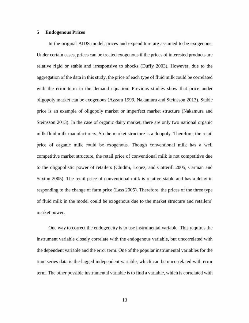
5 Endogenous Prices
In the original AIDS model, prices and expenditure are assumed to be exogenous.
Under certain cases, prices can be treated exogenous if the prices of interested products are
relative rigid or stable and irresponsive to shocks (Duffy 2003). However, due to the
aggregation of the data in this study, the price of each type of fluid milk could be correlated
with the error term in the demand equation. Previous studies show that price under
oligopoly market can be exogenous (Azzam 1999, Nakamura and Steinsson 2013). Stable
price is an example of oligopoly market or imperfect market structure (Nakamura and
Steinsson 2013). In the case of organic dairy market, there are only two national organic
milk fluid milk manufacturers. So the market structure is a duopoly. Therefore, the retail
price of organic milk could be exogenous. Though conventional milk has a well
competitive market structure, the retail price of conventional milk is not competitive due
to the oligopolistic power of retailers (Chidmi, Lopez, and Cotterill 2005, Carman and
Sexton 2005). The retail price of conventional milk is relative stable and has a delay in
responding to the change of farm price (Lass 2005). Therefore, the prices of the three type
of fluid milk in the model could be exogenous due to the market structure and retailers’
market power.
One way to correct the endogeneity is to use instrumental variable. This requires the
instrument variable closely correlate with the endogenous variable, but uncorrelated with
the dependent variable and the error term. One of the popular instrumental variables for the
time series data is the lagged independent variable, which can be uncorrelated with error
term. The other possible instrumental variable is to find a variable, which is correlated with
14
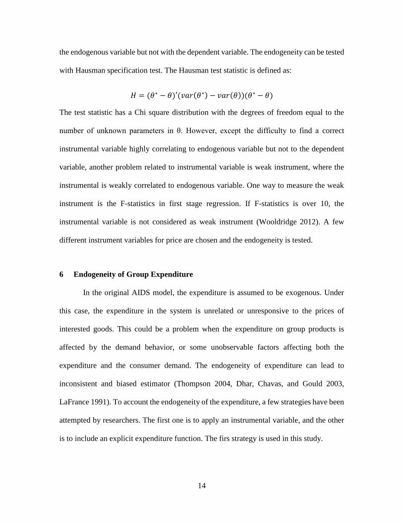
the endogenous variable but not with the dependent variable. The endogeneity can be tested
with Hausman specification test. The Hausman test statistic is defined as:
𝐻 = (𝜃∗ − 𝜃)′(𝑣𝑎𝑟(𝜃∗) − 𝑣𝑎𝑟(𝜃))(𝜃∗ − 𝜃)
The test statistic has a Chi square distribution with the degrees of freedom equal to the
number of unknown parameters in θ. However, except the difficulty to find a correct
instrumental variable highly correlating to endogenous variable but not to the dependent
variable, another problem related to instrumental variable is weak instrument, where the
instrumental is weakly correlated to endogenous variable. One way to measure the weak
instrument is the F-statistics in first stage regression. If F-statistics is over 10, the
instrumental variable is not considered as weak instrument (Wooldridge 2012). A few
different instrument variables for price are chosen and the endogeneity is tested.
6 Endogeneity of Group Expenditure
In the original AIDS model, the expenditure is assumed to be exogenous. Under
this case, the expenditure in the system is unrelated or unresponsive to the prices of
interested goods. This could be a problem when the expenditure on group products is
affected by the demand behavior, or some unobservable factors affecting both the
expenditure and the consumer demand. The endogeneity of expenditure can lead to
inconsistent and biased estimator (Thompson 2004, Dhar, Chavas, and Gould 2003,
LaFrance 1991). To account the endogeneity of the expenditure, a few strategies have been
attempted by researchers. The first one is to apply an instrumental variable, and the other
is to include an explicit expenditure function. The firs strategy is used in this study.

15
7 Unit Root Test Results
Augmented Dickey Fuller (ADF) test is used for the unit root test. Constant and
trend are included in the test. The results show that all series are non-stationary at level but
stationary at the first difference (Table 2 and Table 3). So the next step is to test the
cointegration of the series with Johansen test.
Table 2 Unit Root Test Results for Budget Shares, Prices and Total Expenditure
Variables Label Test
statistics
lag p value Unit
root
Dependent variable
w1 Budget share for conventional whole
milk
-2.8 3 0.188 Yes
w2 Budget share for conventional reduced
fat milk
-3.1 3 0.103 Yes
w3 budget share for organic milk -3.05 2 0.117 Yes
Independent variable
Lnp1 Log price of conventional whole milk -2.23 2 0.471 Yes
Lnp2 Log price of conventional reduced fat
milk
-2.36 2 0.398 Yes
Lnp3 Log price of organic milk -2.75 1 0.214 Yes
LnX Log expenditure of all milk -2.33 2 0.417 Yes
The critical values are -4.055 for 1% and -3.457 for 5% and -3.154 for 10% significant
levels with trend and constant.
16
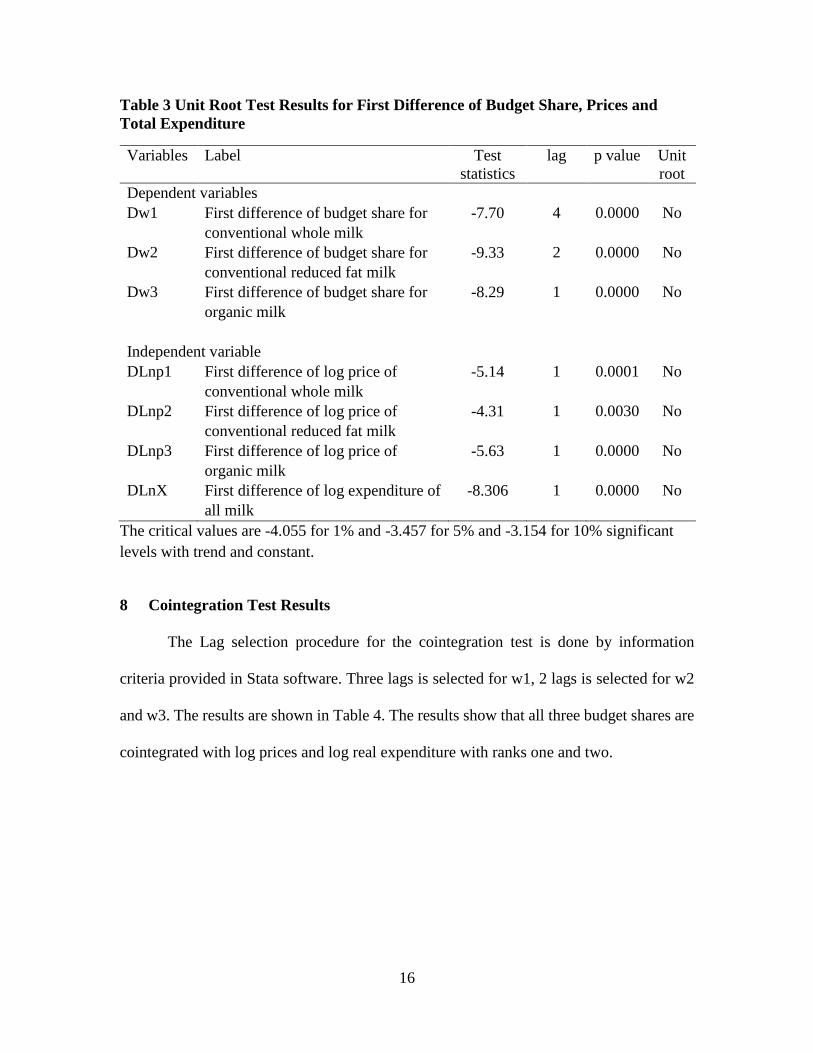
Table 3 Unit Root Test Results for First Difference of Budget Share, Prices and
Total Expenditure
Variables Label Test
statistics
lag p value Unit
root
Dependent variables
Dw1 First difference of budget share for
conventional whole milk
-7.70 4 0.0000 No
Dw2 First difference of budget share for
conventional reduced fat milk
-9.33 2 0.0000 No
Dw3 First difference of budget share for
organic milk
-8.29 1 0.0000 No
Independent variable
DLnp1 First difference of log price of
conventional whole milk
-5.14 1 0.0001 No
DLnp2 First difference of log price of
conventional reduced fat milk
-4.31 1 0.0030 No
DLnp3 First difference of log price of
organic milk
-5.63 1 0.0000 No
DLnX First difference of log expenditure of
all milk
-8.306 1 0.0000 No
The critical values are -4.055 for 1% and -3.457 for 5% and -3.154 for 10% significant
levels with trend and constant.
8 Cointegration Test Results
The Lag selection procedure for the cointegration test is done by information
criteria provided in Stata software. Three lags is selected for w1, 2 lags is selected for w2
and w3. The results are shown in Table 4. The results show that all three budget shares are
cointegrated with log prices and log real expenditure with ranks one and two.
17
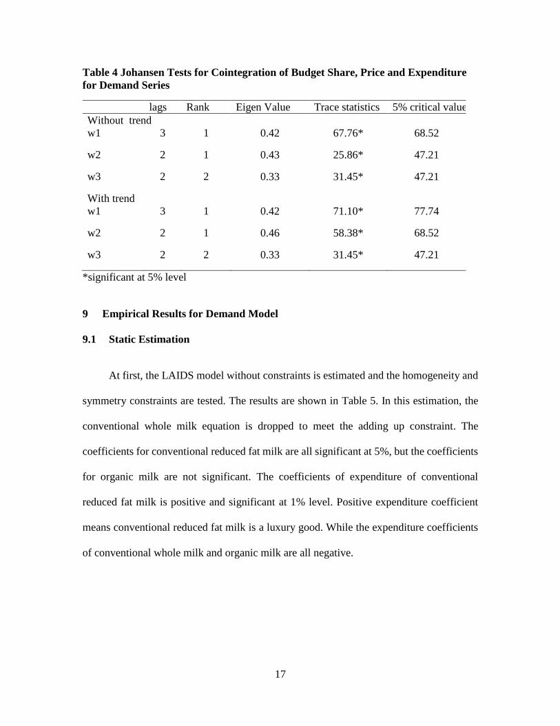
Table 4 Johansen Tests for Cointegration of Budget Share, Price and Expenditure
for Demand Series
lags Rank Eigen Value Trace statistics 5% critical value
Without trend
w1 3 1 0.42 67.76* 68.52
w2 2 1 0.43 25.86* 47.21
w3 2 2 0.33 31.45* 47.21
With trend
w1 3 1 0.42 71.10* 77.74
w2 2 1 0.46 58.38* 68.52
w3 2 2 0.33 31.45* 47.21
*significant at 5% level
9 Empirical Results for Demand Model
9.1 Static Estimation
At first, the LAIDS model without constraints is estimated and the homogeneity and
symmetry constraints are tested. The results are shown in Table 5. In this estimation, the
conventional whole milk equation is dropped to meet the adding up constraint. The
coefficients for conventional reduced fat milk are all significant at 5%, but the coefficients
for organic milk are not significant. The coefficients of expenditure of conventional
reduced fat milk is positive and significant at 1% level. Positive expenditure coefficient
means conventional reduced fat milk is a luxury good. While the expenditure coefficients
of conventional whole milk and organic milk are all negative.
18
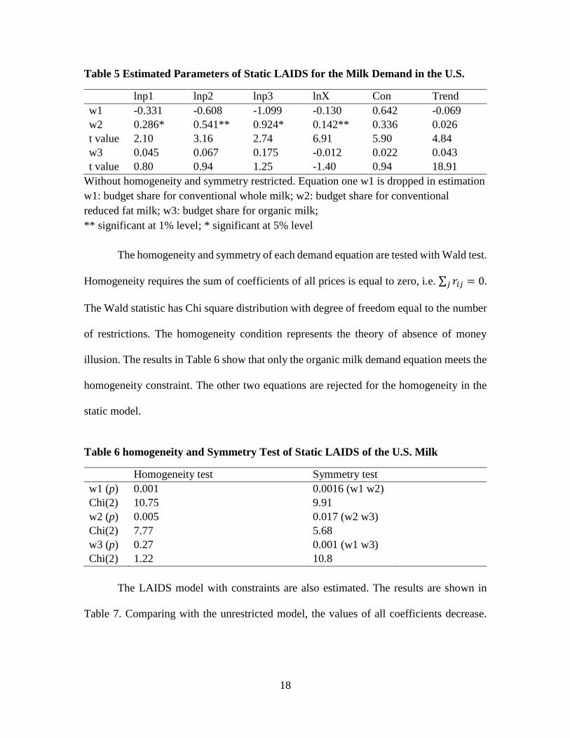
Table 5 Estimated Parameters of Static LAIDS for the Milk Demand in the U.S.
lnp1 lnp2 lnp3 lnX Con Trend
w1 -0.331 -0.608 -1.099 -0.130 0.642 -0.069
w2 0.286* 0.541** 0.924* 0.142** 0.336 0.026
t value 2.10 3.16 2.74 6.91 5.90 4.84
w3 0.045 0.067 0.175 -0.012 0.022 0.043
t value 0.80 0.94 1.25 -1.40 0.94 18.91
Without homogeneity and symmetry restricted. Equation one w1 is dropped in estimation
w1: budget share for conventional whole milk; w2: budget share for conventional
reduced fat milk; w3: budget share for organic milk;
** significant at 1% level; * significant at 5% level
The homogeneity and symmetry of each demand equation are tested with Wald test.
Homogeneity requires the sum of coefficients of all prices is equal to zero, i.e. ∑ 𝑟𝑖𝑗 = 0.𝑗
The Wald statistic has Chi square distribution with degree of freedom equal to the number
of restrictions. The homogeneity condition represents the theory of absence of money
illusion. The results in Table 6 show that only the organic milk demand equation meets the
homogeneity constraint. The other two equations are rejected for the homogeneity in the
static model.
Table 6 homogeneity and Symmetry Test of Static LAIDS of the U.S. Milk
Homogeneity test Symmetry test
w1 (p) 0.001 0.0016 (w1 w2)
Chi(2) 10.75 9.91
w2 (p) 0.005 0.017 (w2 w3)
Chi(2) 7.77 5.68
w3 (p) 0.27 0.001 (w1 w3)
Chi(2) 1.22 10.8
The LAIDS model with constraints are also estimated. The results are shown in
Table 7. Comparing with the unrestricted model, the values of all coefficients decrease.

19
Only two parameters, organic milk price in organic milk budget share and real expenditure
of reduced fat milk are statistically significant at the 5% level.
Table 7 Estimated Parameters of Static LAIDS for the Milk Demand in the U.S.
lnp1 lnp2 lnp3 lnX Con Trend
w1 0.077 - -0.139 0.484 -0.075
w2 -0.069 0.084 0.150** 0.472 0.032
t value -1.43 1.54 7.07 5.80 6.18
w3 -0.007 -0.014 0.022** -0.011 0.045 0.044
t value -0.68 -0.36 4.24 -1.26 3.80 20.27
With homogeneity and symmetry restricted. Equation one is dropped for estimation
** significant at 1% level
9.2 Dynamic Estimation with Vector Error Correction Model
Time plays important factor in demand analysis since consumer preference, price
and income (expenditure on milk) subject to change with time. The homogeneity and
symmetry are rejected in the static model. Deaton and Muellbauer (1980) and Duffy (2003)
state that the rejection of the constraints is due to the misspecification of a dynamic model
in a static one. So, the next step is to build a dynamic model to incorporate long and short-
run effects. In the dynamic model, two lagged budget shares are included to represent the
habit persistence (the number of lags is determined by the information criteria in Stata).
The error correction term is estimated from the lagged residual of OLS regression of the
static demand system, because the coefficients of OLS are consistent. At the first, the
unrestricted dynamic model is estimated and the results are shown in Table 8. The
coefficients of lagged dependent variable and error correct term in conventional reduced
fat milk and error correct term of organic milk are significant at 1% or 5% level in the
unrestricted dynamic model. Both error correction terms of organic milk and conventional
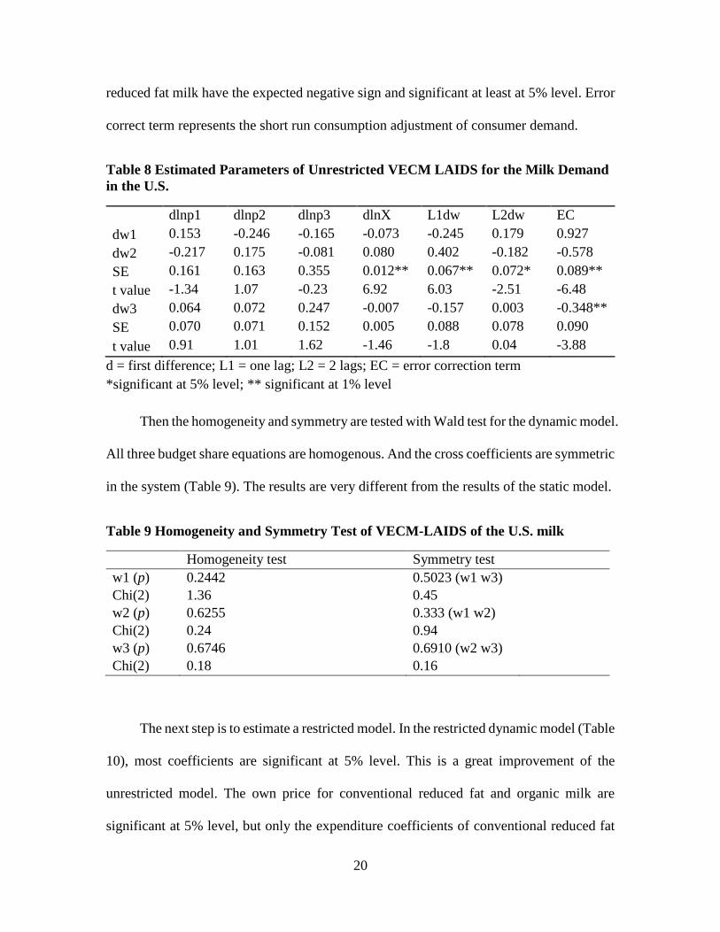
20
reduced fat milk have the expected negative sign and significant at least at 5% level. Error
correct term represents the short run consumption adjustment of consumer demand.
Table 8 Estimated Parameters of Unrestricted VECM LAIDS for the Milk Demand
in the U.S.
dlnp1 dlnp2 dlnp3 dlnX L1dw L2dw EC
dw1 0.153 -0.246 -0.165 -0.073 -0.245 0.179 0.927
dw2 -0.217 0.175 -0.081 0.080 0.402 -0.182 -0.578
SE 0.161 0.163 0.355 0.012** 0.067** 0.072* 0.089**
t value -1.34 1.07 -0.23 6.92 6.03 -2.51 -6.48
dw3 0.064 0.072 0.247 -0.007 -0.157 0.003 -0.348**
SE 0.070 0.071 0.152 0.005 0.088 0.078 0.090
t value 0.91 1.01 1.62 -1.46 -1.8 0.04 -3.88
d = first difference; L1 = one lag; L2 = 2 lags; EC = error correction term
*significant at 5% level; ** significant at 1% level
Then the homogeneity and symmetry are tested with Wald test for the dynamic model.
All three budget share equations are homogenous. And the cross coefficients are symmetric
in the system (Table 9). The results are very different from the results of the static model.
Table 9 Homogeneity and Symmetry Test of VECM-LAIDS of the U.S. milk
Homogeneity test Symmetry test
w1 (p) 0.2442 0.5023 (w1 w3)
Chi(2) 1.36 0.45
w2 (p) 0.6255 0.333 (w1 w2)
Chi(2) 0.24 0.94
w3 (p) 0.6746 0.6910 (w2 w3)
Chi(2) 0.18 0.16
The next step is to estimate a restricted model. In the restricted dynamic model (Table
10), most coefficients are significant at 5% level. This is a great improvement of the
unrestricted model. The own price for conventional reduced fat and organic milk are
significant at 5% level, but only the expenditure coefficients of conventional reduced fat
21
milk is significant at 1% level. The first lags of budget shares are significant. The error
correction terms in organic milk and conventional reduced fat milk demand equations have
expected negative sign and statistically significant. The conventional whole milk has
positive sign for error correction term. This is due to the adding up constraints. The signs
of the own prices in all three equations are as expected positive. Comparing with the static
model, the own prices have the same sign, but the coefficients in the dynamic model are
larger than the ones in the static model.
9.3 Dynamic Model with Instrument Variables
The lagged prices are first adopted as an instrument for endogenous prices. The
Hausman-Wu test fails to reject the null hypothesis that three prices are exogenous. The
partial R2 of the lagged endogenous variables in the first stage regression is around 50%,
and the partial F statistics is about 25 (F-statistics is over 10 for the standard). So this is not
a weak instrument.
The second possible instrument variable for organic milk price is the price of organic
feed, which is closely related to retail price, but not related to consumer demand. However,
the data are not available. Therefore, the organic egg retail price is adopted for the organic
milk price, because organic egg is a subsector of organic dairy. The Hausman-Wu test
shows that the hypothesis that organic milk price is exogenous is rejected at 1% level. The
F-statistic for the first stage is 15 and the first stage partial R2 is 14%, which is relative
small. The instrumental variable only weakly correlates with the endogenous variable. The
instrument variables used for conventional milk are U.S. monthly feed corn price and
sorghum price. However, these two instrumental variables have very low correlation with
22
the endogenous variables and are weak instruments. Weak instrumental variables also can
lead to inconsistent and biased estimator. Based on the last two tests, the exogenous prices
are assumed in the study.
In the test of endogeneity of group expenditure, the real disposable income is selected
as an instrumental variable. The results show that the null hypothesis, the expenditure is
exogenous is rejected, and the null hypothesis that instruments are weak also is rejected.
The partial F-statistic is 22 and significant at 5% level. Therefore, the income deflated with
price index is used as an instrument for group expenditure.
The right side of Table 10 shows the regression results of dynamic model with
instrument variable for expenditure. In this model, almost all coefficients decreased from
the left side dynamic model without instrument. One big difference from the model without
instrument is that the signs of expenditure change to opposite. In the conventional reduced
fat milk equation, the coefficient of expenditure changes from significant positive to
insignificant negative. In the organic milk equation, the coefficient of expenditure changes
from insignificant negative to significant positive. From this model organic milk is a
luxury goods and conventional reduced fat is a necessary goods. This confirms with our
perception. However, last month consumption difference has negative effect on budget
share of organic milk but positive for conventional reduced fat milk. The coefficients of
error correction terms in organic and conventional reduced fat milk have the expected
negative sign, and have little change (-0.329 to -0.340) in organic milk equation from the
model without instrument.

23
Table 10 Estimated Parameters of Restricted VECM LAIDS for the Milk Demand in the U.S.
VECM-AIDS VECM-AIDS with instrument
dlnp1 dlnp2 dlnp3 dlnX L1dw L2dw EC dlnp1 dlnp2 dlnp3 dlnX L1dw L2dw EC
dw1 0.213 -0.186 -0.027 -0.072 -0.223 0.194 0.901 0.254 -0.215 -0.039 -0.017 -0.150 0.253 0.778
dw2 -0.186* 0.203** -0.017 0.080** 0.404** -0.183* -0.572* -0.215* 0.202* 0.014 -0.055 0.315** -0.244* -0.439**
SE 0.046 0.053 0.016 0.012 0.065 0.072 0.088 0.074 0.093 0.029 0.102 0.078 0.088 0.106
t value -4.04 3.87 -1.03 6.92 6.22 -2.54 -6.52 -2.92 2.18 0.47 -0.54 4.05 -2.78 -4.16
dw3 -0.027* -0.017 0.044** -0.007 -0.181* -0.011 -0.329* -0.039 0.014 0.026* 0.073* -0.165* -0.009 -0.340**
SE 0.014 0.016 0.008 0.005 0.086 0.078 0.089 0.021 0.029 0.013 0.037 0.085 0.075 0.087*
t value -1.96 -1.03 5.13 -1.5 -2.12 -0.14 -3.68 -1.86 0.47 2.02 1.93 -1.94 -0.13 -3.89
* Equation with w1 was dropped in estimation.
24
9.4 Elasticity
9.4.1 Price Elasticity from the Static Model
Price elasticities calculated with unconstrained static model do not have expected
signs (not shown here). Therefore, the price and expenditure elasticities are calculated with
coefficients from the restricted model. The uncompensated elasticities on the left of Table
11 for all three types of milk have expected negative signs. However, the elasticity of
conventional reduced fat milk is even higher than the one of organic milk, which is not as
expected. Both organic and conventional whole milk have elasticities less than one, but the
conventional reduced fat milk has elasticity close to one. The cross price elasticity between
conventional whole milk and conventional reduced milk shows that they are complements.
Organic milk and reduced fat conventional milk are also complements.
Comparing with the uncompensated elasticity, the compensated elasticity (Table
12) of conventional reduced fat decreases significantly from -1.022 to -0.218, smaller than
the elasticities of conventional whole milk and organic milk. The changes of elasticities of
conventional whole and organic milk are small relative to conventional reduced fat milk.
This is because of the large budget share of conventional reduced fat milk (the budget share
in the formula of compensated elasticity). Organic milk has the largest compensated price
elasticity, but still less than one and inelastic.
9.4.2 Price Elasticity from Dynamic Models
The uncompensated and compensated elasticities of all three goods in the dynamic
model are shown in Table 11 and Table 12. The uncompensated price elasticities in the
dynamic model without instrument are smaller than the values in the static model. The
25
dynamic model with instrument has largest absolute own price elasticity for organic milk
-0.714 vs -0.382 and -0.628 in dynamic model with no instrument and static model. The
own price elasticity of conventional reduced fat milk in dynamic model is the largest in all
three models, but close to the value in the dynamic model with instrument. This is because
the coefficients in the two dynamic models are close.
Regarding to the compensated price elasticities, the absolute values are smaller than
the corresponding uncompensated elasticities in all three models. In the dynamic model,
the consumption of conventional whole and reduced fat milk almost have no response to
the price change (0.052, 0.037 elasticities for conventional whole and reduced fat milk
respectively), and organic milk has somewhat response (-0.318 in dynamic with no
instrument, and -0.517 in dynamic with instrument), but all elasticities are inelastic. In the
dynamic models, three types of milk are complements, because the cross price elasticities
are negative.
26
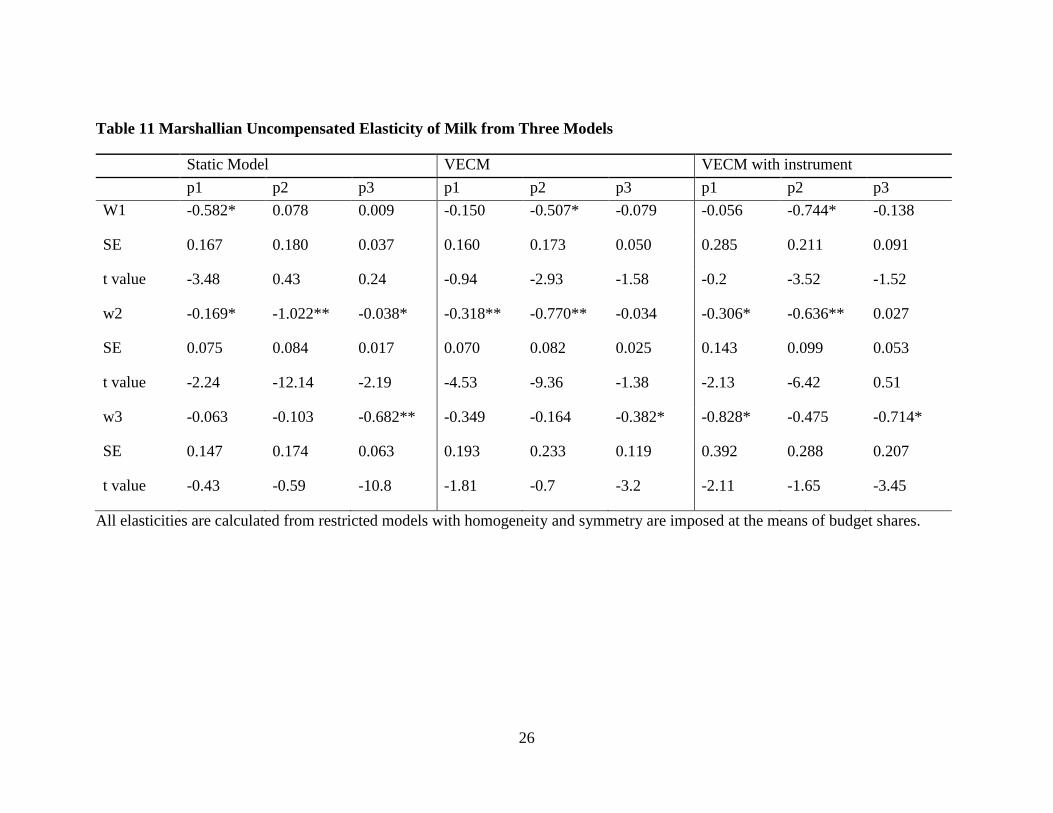
Table 11 Marshallian Uncompensated Elasticity of Milk from Three Models
All elasticities are calculated from restricted models with homogeneity and symmetry are imposed at the means of budget shares.
Static Model VECM VECM with instrument
p1 p2 p3 p1 p2 p3 p1 p2 p3
W1 -0.582* 0.078 0.009 -0.150 -0.507* -0.079 -0.056 -0.744* -0.138
SE 0.167 0.180 0.037 0.160 0.173 0.050 0.285 0.211 0.091
t value -3.48 0.43 0.24 -0.94 -2.93 -1.58 -0.2 -3.52 -1.52
w2 -0.169* -1.022** -0.038* -0.318** -0.770** -0.034 -0.306* -0.636** 0.027
SE 0.075 0.084 0.017 0.070 0.082 0.025 0.143 0.099 0.053
t value -2.24 -12.14 -2.19 -4.53 -9.36 -1.38 -2.13 -6.42 0.51
w3 -0.063 -0.103 -0.682** -0.349 -0.164 -0.382* -0.828* -0.475 -0.714*
SE 0.147 0.174 0.063 0.193 0.233 0.119 0.392 0.288 0.207
t value -0.43 -0.59 -10.8 -1.81 -0.7 -3.2 -2.11 -1.65 -3.45

27
Table 12 Hickman Compensated Elasticity for Milk from Three Models
Static model VECM-AIDS VECM with instrument
p1 p2 p3 p1 p2 p3 p1 p2 p3
w1 -0.446* 0.402* 0.044 0.052 -0.025 -0.027 0.201 -0.130 -0.071
SE 0.164 0.177 0.037 0.161 0.168 0.050 0.231 0.269 0.076
t value -2.72 2.28 1.2 0.32 -0.15 -0.54 0.87 -0.49 -0.93
w2 0.169* -0.218* 0.049* -0.010 -0.036 0.046 -0.055 -0.037 0.092*
SE 0.074 0.083 0.017 0.071 0.080 0.025 0.113 0.141 0.044
t value 2.28 -2.63 2.85 -0.15 -0.44 1.87 -0.49 -0.26 2.08
w3 0.170 0.452* -0.622** -0.104 0.422 -0.318* -0.274 0.844* -0.571*
SE 0.141 0.159 0.063 0.193 0.226 0.119 0.294 0.406 0.177
t value 1.2 2.85 -9.9 -0.54 1.87 -2.67 -0.93 2.08 -3.22
All elasticities are calculated from restricted models with homogeneity and symmetry are imposed at the means of budget shares.

28
9.4.3 Expenditure Elasticity
The expenditure elasticities for all milk are significant at 1% level in all three
models (Table 13). Conventional reduced fat has the highest expenditure elasticity and
greater than one in the models of static and dynamic model without instrument. In the
instrumented dynamic model, the organic milk is expenditure elastic and conventional milk
has almost unit expenditure elasticity. For organic milk, 1% increase in total milk
expenditure will increase organic milk consumption by 2%. This confirms organic milk is
a luxury good.
Table 13 Estimated Expenditure Elasticities from Three Models
9.5 Habit Formation
There are different ways to model the dynamic time effect in a model. One of the
methods is to use lagged consumption quantity in the model, and the other is to use lagged
dependent variable, budget share. In the dynamic model, the coefficients of lagged budget
shares of conventional reduced fat milk and organic milk are significant at the 5% level. In
conventional reduced fat model, previous two periods consumptions have different effects
on the current consumption. Immediate past consumption has positive effect on current
effect, but consumption of two months ago has negative effect on current consumption. For
Static model VECM Instrument VECM
w1 w2 w3 w1 w2 w3 w1 w2 w3
Elasticity 0.495 1.229 0.848 0.737 1.122 0.895 0.937 0.915 2.017
SE 0.077 0.032 0.119 0.039 0.018 0.070 0.303 0.157 0.526
t value 6.4 38.01 7.15 18.88 63.69 12.77 3.1 5.84 3.84

29
organic milk, consumptions in previous two months have negative effects on current
consumption.
10 Summary and Conclusion
The objective of this study is to incorporate the time series property of the data and
develop a VEC-LAIDS model for conventional whole, reduced fat milk and organic milk.
This is the first paper to apply time series techniques in the demand analysis of organic
milk. In addition, the study updates the organic milk consumption data to 2013, while most
recent study was done with data in 2010 or before.
Organic milk consumption is still a small portion of the entire fluid milk
consumption, 3% of volume and 7% of expenditure. The retail price of organic milk is two
times of conventional milk. The consumption of the organic milk and reduced fat
conventional milk have increased in the period, but the consumption of conventional whole
milk has decreased.
The time series data are non-stationary and integrated at the degree one. The budget
shares are cointegrated with log price and log expenditure. The estimated coefficients from
the static and dynamic models have large differences, especially for the price elasticity.
The results in both models show that conventional and organic milk are price inelastic, and
the expenditure elasticities of conventional milk are close to unit, but organic milk could
be up to 2.0 in the instrumented dynamic model. In the dynamic model, the demand of
conventional milk is almost irresponsive to the price change. The dynamic model shows
that the consumption pattern does affect the demand of milk or the persistence of
consumption. Comparing with the static model, the dynamic model meets both
30
homogeneity and symmetry constraints, while the static model does not meet these
constraints.
In both static and dynamic models, the compensated price elasticity has large
difference from uncompensated elasticity. The results show organic milk has larger own
price elasticity than conventional milk, but it is still inelastic, -0.714. This could be true to
the committed organic milk consumers, or consumers who only consume organic milk.
This elasticity is the lowest comparing with all current studies of organic milk demand
(Alviola and Capps 2010, Chang et al. 2011, Choi, Wohlgenant, and Zheng 2013, Glaser
and Thompson 2000, Li, Peterson, and Tian 2012, Chikasada 2008, Dhar and Foltz 2005).
The closest elasticity is -0.802 in Chang (2011). The highest elasticity is -9.7 in Glaser and
Thompson (2000), who found the price elasticity decreased with time. The most recent
data set is from Li, Peterson and Tian (2012), in which supermarket weekly scanner data
from 2008-2010 were used. In this study, the elasticities for organic milk with different fat
contents are from -1.046 to -1.598, and organic whole milk has the lowest own price
elasticity among all organic milk. However, time series property is not considered in this
study.
The compensated own price elasticities of the conventional milk (-0.021 for
conventional whole, and -0.037 for conventional reduced fat in dynamic model with
instrument) are lower than the elasticities in all current studies. The low compensated
elasticity means that with income compensated, the price has no effects on consumer
demand of conventional milk. This is in line with consumption pattern of milk.

31
In the dynamic model without instrument, the expenditure elasticities of organic
milk and conventional whole milk are inelastic, and the expenditure elasticity of
conventional reduced fat is over one, 1.122. The expenditure elasticity of organic milk
(0.895) is in the range of elasticities of current studies (from -8.6 to 0.871). This elasticity
is close to the study of Li, Peterson and Tian (2012), 0.871, while the elasticity of organic
milk in the dynamic model with instrument is 2.0 and elastic.
Demand analysis especially the price elasticity is important for the marketing and
pricing strategy. Conventional and organic milk manufacturers and retailers can use the
price elasticity information to direct their production, sales and marketing. Milk retailers
also can use the price elasticity to set up their pricing strategy to increase their sales and
revenue. Since organic milk is price inelastic overall for the aggregated data, retailers can
increase the price of organic milk for high revenue as of conventional milk, especially
when the consumers are committed organic milk drinkers. On the other hand, organic milk
is expenditure elastic. High income consumers may purchase more organic milk than the
consumers with relative lower income. Retailers may target their sales to different types of
consumers for organic and conventional milk.
Other factors such as demographic variables, forecast and simulation need to be
considered in the demand model. These will be investigated in the future research.
11 Reference
Alviola, Pedro A., and Oral Capps. 2010. "Household demand analysis of organic and
conventional fluid milk in the United States based on the 2004 Nielsen Homescan
panel." Agribusiness 26 (3):369-388. doi: 10.1002/agr.20227.
Azzam, Azzeddine M. 1999. "Asymmetry and rigidity in farm-retail price transmission."
American journal of agricultural economics 81 (3):525-533.
32
Carman, Hoy F, and Richard J Sexton. 2005. "Supermarket fluid milk pricing practices in
the Western United States." Agribusiness 21 (4):509-530.
Chang, Ching-Hsing, Neal H. Hooker, Eugene Jones, and Abdoul Sam. 2011. "Organic
and conventional milk purchase behaviors in Central Ohio." Agribusiness 27
(3):311-326. doi: 10.1002/agr.20269.
Chidmi, Benaissa, Rigoberto A Lopez, and Ronald W Cotterill. 2005. "Retail oligopoly
power, dairy compact, and Boston milk prices." Agribusiness 21 (4):477-491.
Chikasada, Mitsuko. 2008. "Three essays on demand for organic milk in the U.S.,
environment and economic growth in Japan, and life expectancy at birth and socio-
economic factors in Japan." 3441052 Ph.D., The Pennsylvania State University.
Choi, Hee-Jung, Michael K. Wohlgenant, and Xiaoyong Zheng. 2013. "Household-Level
Welfare Effects of Organic Milk Introduction." American Journal of Agricultural
Economics 95 (4):1009-1028.
Davis, Christopher, Donald Blayney, Joseph Cooper, and Steven Yen. 2009. "An Analysis
of Demand Elasticities for Fluid Milk Products in the US." International
Association of Agricultural Economists Meeting, August.
Deaton, Angus, and John Muellbauer. 1980. "An almost ideal demand system." The
American economic review 70 (3):312-326.
Dhar, Tirtha, Jean-Paul Chavas, and Brian W Gould. 2003. "An empirical assessment of
endogeneity issues in demand analysis for differentiated products." American
Journal of Agricultural Economics 85 (3):605-617.
Dhar, Tirtha, and Jeremy D Foltz. 2005. "Milk by any other name… consumer benefits
from labeled milk." American Journal of Agricultural Economics 87 (1):214-228.
Dimitri, Carolyn, and Kathryn M. Venezia. 2007. "Retail and consumer aspects of the
organic milk market [electronic resource] / Carolyn Dimitri and Kathryn M.
Venezia." In.: [Washington, D.C.] : U.S. Dept. of Agriculture, Economic Research
Service, [2007].
Duffy, Martyn. 2003. "Advertising and food, drink and tobacco consumption in the United
Kingdom: a dynamic demand system." Agricultural Economics 28 (1):51-70.
Gardner, Bruce L. 1975. "The farm-retail price spread in a competitive food industry."
American Journal of Agricultural Economics 57 (3):399-409.
Glaser, Lewrene K, and Gary D Thompson. 2000. "Demand for organic and conventional
beverage milk." Selected Paper presented at Annual Meeting of the Western
Agricultural Economics Association, Vancouver, British Columbia.
LaFrance, Jeffrey T. 1991. "When is expenditure" exogenous" in separable demand
models?" Western Journal of Agricultural Economics:49-62.
Lass, Daniel A. 2005. "Asymmetric response of retail milk prices in the northeast
revisited." Agribusiness 21 (4):493-508.
Li, Xianghong, H. H. Peterson, and Xia Tian. 2012. "U.S. consumer demand for organic
fluid milk by fat content." Journal of Food Distribution Research 43 (1):50-58.
Nakamura, Emi, and Jón Steinsson. 2013. Price rigidity: Microeconomic evidence and
macroeconomic implications. National Bureau of Economic Research.
Organic Trade Association. 2012. "Consumer-driven U.S. organic market surpasses $31
billion in 2011."
http://www.organicnewsroom.com/2012/04/us_consumerdriven_organic_mark.ht
ml.
33
Schrimper, Ronald A. 1995. "Subtleties Associated With Derived Demand Relationships."
Agricultural and Resource Economics Review 24:241-246.
Siemon, George L. 2010. "Organic Dairy Market also Hurt by Low Prices." Rural
Cooperatives (January/Februrary):15,-38.
Thompson, Wyatt. 2004. "Using Elasticities from an Almost Ideal Demand System? Watch
Out for Group Expenditure!" American Journal of Agricultural Economics 86
(4):1108-1116. doi: 10.1111/j.0002-9092.2004.00656.x.
Wooldridge, Jeffrey. 2012. Introductory econometrics: A modern approach: Cengage
Learning.
Duffy, M. (2003). "On the estimation of an advertising-augmented, cointegrating demand
system." Economic Modelling 20(1): 181-206.