Embed Size (px)
Citation preview

Statistica Sinica 21 (2011), 1145-1170
A TWO-STAGE ESTIMATION METHOD FOR RANDOM
COEFFICIENT DIFFERENTIAL EQUATION MODELS
WITH APPLICATION TO LONGITUDINAL
HIV DYNAMIC DATA
Yun Fang, Hulin Wu and Li-Xing Zhu
Shanghai Normal University, University of Rochesterand Hong Kong Baptist University
Abstract: We propose a two-stage estimation method for random coefficient ordi-
nary differential equation (ODE) models. A maximum pseudo-likelihood estimator
(MPLE) is derived based on a mixed-effects modeling approach and its asymptotic
properties for population parameters are established. The proposed method does
not require repeatedly solving ODEs, and is computationally efficient although it
does pay a price with the loss of some estimation efficiency. However, the method
does offer an alternative approach when the exact likelihood approach fails due to
model complexity and high-dimensional parameter space, and it can also serve as a
method to obtain the starting estimates for more accurate estimation methods. In
addition, the proposed method does not need to specify the initial values of state
variables and preserves all the advantages of the mixed-effects modeling approach.
The finite sample properties of the proposed estimator are studied via Monte Carlo
simulations and the methodology is also illustrated with application to an AIDS
clinical data set.
Key words and phrases: AIDS/HIV data, local polynomial kernel smoothing, lon-
gitudinal data, mixed-effects models, ordinary differential equation, pseudo likeli-
hood, viral dynamics.
1. Introduction
Ordinary differential equation (ODE) models are widely used in such scien-tific fields as engineering, physics, econometrics, and, recently, biomedical sci-ences. ODE models have been applied to quantify HIV viral dynamics and haveled to many important findings for AIDS pathogenesis in the past two decades(Ho et al. (1995), Perelson et al. (1996), Perelson et al. (1997), Perelson andNelson (1999), Wu et al. (1999), Wu and Ding (1999), Nowak and May (2000),Tan and Wu (2005), and Wu (2005)).
In this paper, we use a two-stage method to estimate the random coefficientparameters in ODE models for longitudinal data. In the first stage, we estimate

1146 YUN FANG, HULIN WU AND LI-XING ZHU
the state variables and time-varying covariates, as well as their derivatives, by us-ing local polynomial smoothing for the nonparametric mixed effects models (Wuand Zhang (2002)). In the second stage, a maximum pseudo-likelihood (MPL)estimation is developed to estimate the unknown parameters, including both thepopulation and individual coefficients in a random coefficient ODE model. Theasymptotic properties of the proposed estimator for population parameters areestablished. The spirit of two-stage method was initiated by Varah (1982) whoused a cubic spline to smooth the data in the first stage, and employed the leastsquares method for parameter estimation in the second stage. Ellner, Seifu, andSmith (2002) fitted the dynamic models to time series data using the local poly-nomial regression. Liang and Wu (2008) established the theoretical propertiesof the method for ODE models by applying the local polynomial smoothing inthe first stage. They proved that the two-step estimator has strong consistencyand asymptotic normality. Brunel (2008) obtained similar asymptotic results byusing regression splines. Chen and Wu (2008a,b) adopted a similar two-stagemethod for ODE models with time-varying coefficients and also obtained theasymptotic results for the proposed estimators. However, this literature dealsonly with cross-section iid data.
Longitudinal dynamic systems (random coefficient ODE models) have beensuggested by Putter et al. (2002), Huang and Wu (2006), and Huang, Liu, and Wu(2006), in which the hierarchical Bayesian approach was used to estimate dynamicparameters in HIV dynamic models from longitudinal clinical data. Lahiri (2003)proposed a spline-enhanced population model to study pharmacokinetics using arandom time-varying coefficient ODE model. Guedj, Thiebaut, and Commenges(2007) used the maximum likelihood approach directly to estimate unknownparameters in random coefficient ODE models.
In this paper, we extend the two-step estimation method (Varah (1982),Liang and Wu (2008)) to longitudinal dynamic systems by adopting the mixed-effects modeling approach. The extension is not trivial. When the nonparametricmixed-effects (NPME) modeling approach is used in the first step, we need toresort to asymptotic independence and a pseudo-likelihood idea to derive theparameter estimates in the second step. The asymptotic theories for the proposedpseudo-likelihood estimator are established. We also demonstrate, via MonteCarlo simulations, that the NPME modeling approach in the first step providesa good estimate for the state variables and their derivatives. Thus, the proposedmethod preserves the advantages of both the mixed-effects modeling approachand the two-step estimation method for ODE models: it avoids repeatedly solvingthe ODE numerically so that it is computationally efficient; it does not require

A TWO-STAGE ESTIMATION METHOD 1147
initial values of state variables; and implementation is easy compared to the exactmaximum likelihood method for ODE models.
The remainder of this paper is organized as follows. The two-stage esti-mation procedure is described in Section 2. The theoretical properties for thepopulation estimates are established in Section 3. In Section 4, we fit a viraldynamic model to a longitudinal HIV dynamic data from an AIDS clinical studyto further illustrate the usefulness of the proposed method. In Section 5, we con-duct simulation studies to evaluate the performance of the proposed estimates.We conclude our paper with some discussion in Section 6. The proofs of thetheoretical results are provided in the Appendix.
2. Estimation Procedure
The proposed method is motivated by a HIV dynamic study with a popularODE model:
d
dtTU (t) = λ − ρTU (t) − η(t)TU (t)V (t),
d
dtTI(t) = η(t)TU (t)V (t) − δTI(t), (2.1)
d
dtV (t) = NδTI(t) − cV (t),
where TU (t) is the concentration of uninfected target T cells, TI(t) is the con-centration of infected cells, and V (t) is the concentration of plasma virus (viralload) at time t. The functions V (t), TU (t), and TI(t) are called state variables.Parameter λ represents the rate at which new T cells are continuously generated,ρ is the death rate of uninfected T cells, η(t) is the time-varying infection rate ofT cells, δ is the death rate of infected cells, c is the clearance rate of free virus,and N is the average number of virus produced from each infected cell.
In the dynamic system (2.1), viral load V (t) and total CD4+ T cell countsT (t) = TU (t)+TI(t) can be measured in AIDS clinical studies. Using some simplealgebra, Liang and Wu (2008) transformed the system (2.1) into a single ODEmodel:
V ′(t) = α0 + α1T (t) + α2T′(t) − cV (t), (2.2)
where V ′(t) = dV (t)/dt and T ′(t) = dT (t)/dt, and parameters α0 = −Nδλ/(ρ−δ), α1 = −Nδρ/(ρ − δ) and α2 = Nδ/(ρ − δ). Model (2.2) can be extended intoa random coefficient ODE model as
V ′i (tij) = α0i + α1iTi(tij) + α2iT
′i (tij) − ciVi(tij), (2.3)

1148 YUN FANG, HULIN WU AND LI-XING ZHU
with subject index i = 1, . . . , n and the measurement index for the ith subjectj = 1, . . . , ni. In general, model (2.3) can be written as
X ′i(tij) = F (Xi(tij), Zi(tij), Z ′
i(tij), θi)τ , i = 1, . . . , n, j = 1, . . . , ni, (2.4)
where Xi is a vector of state variables for the ith subject. The vector Zi(tij) =(Zi1(tij), . . . , Zik(tij))τ is a k×1 vector of input variables (covariates) and Z ′
i(tij)denotes its derivative (the notation “τ” stands for transposition). F (·) = (F1(·),. . . , Fq(·))τ is a known linear or nonlinear function vector. The random coefficient(unknown parameter) vector can be written as θi = θ + bθ,i, where θ (q × 1)is the population parameter vector and bθ,i’s are random components of theparameters that are independent and identically distributed (i.i.d.) with mean0 and covariance matrix Dθ. For simplicity, we only consider the case that Xi
is a univariate state variable and the ODE model (2.4) is linear for unknownparameters θi, i.e., the linear mixed-effects ODE model
X ′i(tij) = F (Xi(tij), Zi(tij), Z ′
i(tij))τθi, i = 1, . . . , n, j = 1, . . . , ni. (2.5)
Note that (2.5) has no closed-form solution in general. Although the theoret-ical results are difficult to establish and the computation is more costly, ourmethodologies are applicable to general nonlinear mixed-effects ODE models(models with nonlinear for unknown parameters). In this paper, for simplicity,our methodology and theoretical development focus on model (2.5).
In model (2.5), the state variable Xi(t) and input variables Zil(t), for 1 ≤l ≤ k, are observed longitudinally, i.e., for i = 1, . . . , n, j = 1, . . . , ni,
Yi(tij) = Xi(tij) + εi(tij), Xi(tij) = u(tij) + vi(tij), (2.6)
Sil(tij) = Zil(tij) + εil(tij), Zil(tij) = ul(tij) + vil(tij), (2.7)
where u(t) and ul(t) are the population mean (fixed-effect) functions of the lon-gitudinal data; vi(t) and vil(t), which are the subject-specific effects or random-effect functions, model the departure of the i-th individual effect from the pop-ulation mean functions u(t) and ul(t), respectively, and εi(t) and εil(t) are themeasurement error functions, respectively. Models (2.6) and (2.7) can be con-sidered as nonparametric mixed-effects (NPME) models (Shi, Weiss, and Taylor(1996), Rice and Wu (2001), and Wu and Zhang (2002, 2006)).
In the following subsections, we introduce the two-stage estimation procedurefor the random coefficient ODE model (2.5). The basic idea is to apply a non-parametric smoothing approach to (2.6) and (2.7) to estimate the time-varyingstate variables and input variables (covariates) as well as their derivatives in thefirst stage, and then substitute the estimates from the first stage to model (2.5)to form a parametric regression model to estimate unknown parameters in thesecond stage.

A TWO-STAGE ESTIMATION METHOD 1149
2.1. Stage I: nonparametric estimation of state variables and theirderivatives
In the first stage, we fit the NPME model (2.6) and (2.7) to obtain theestimates of the time-varying state variables, Xi(t), and the input variables, Zi(t),as well as their derivatives for each individual subject using the local polynomialapproach (Wu and Zhang (2002)). Here we only present the results for the statevariable Xi(t), it is the same for the input variable Zi(t). For convenience, weassume that the unobserved random-effect functions vi(t) are i.i.d. samplingtrajectories of the underlying Gaussian process (GP) with mean function 0 anda covariance function γ(s, t). We also assume that the measurement errors εi(t)are i.i.d. copies of a GP ε(t) with mean 0 and a covariance function γε(s, t) =σ2(t)I(s = t), where I(·) is an index function. For i = 1, . . . , n, we have
vi ∼ GP (0, γ), εi ∼ GP (0, γε). (2.8)
Let tij , j = 1, . . . , ni be the design time points for the ith individual subject.The model (2.6) can be rewritten as
Yij = u(tij) + vi(tij) + εi(tij), i = 1, . . . , n, j = 1, . . . , ni. (2.9)
Assume that u(t) and vi(t) are smooth functions and have up to (p + 1)-ordercontinuous derivatives at each time point within some interval of interest, v
(r)i (t)
with covariance function γr(t, s), for each r = 1, . . . , p. Then, for each tij , u(tij)and vi(tij) can be approximated by p-th degree polynomials within a neighbor-hood of t0, i.e.,
u(tij) ≈ u(t0) + u′(t0)(tij − t0) + . . . +u(p)(t0)
p!(tij − t0)p = Hτ
ij,p(t0)β, (2.10)
vi(tij) ≈ vi(t0) + v′i(t0)(tij − t0) + . . . +v
(p)i (t0)
p!(tij − t0)p = Hτ
ij,p(t0)bi, (2.11)
where Hij,p(t0) = (1, (tij − t0), . . . , (tij − t0)p)τ , and
β =[u(t0), u′(t0), . . . ,
u(p)(t0)p!
]τ, bi =
[vi(t0), v′i(t0), . . . ,
v(p)i (t0)
p!
]τ. (2.12)
Thus, within a neighborhood of t0, the NPME model (2.9) can be approximatedby a LME model
Yij = Hτij,p(t0)β + Hτ
ij,p(t0)bi + εij , i = 1, . . . , n, j = 1, . . . , ni, (2.13)
where εij include the measurement and approximation errors, and bi are therandom effects. Let Kh(·) = K(·/h)/h, K a kernel function and h denoting

1150 YUN FANG, HULIN WU AND LI-XING ZHU
bandwidth. For model (2.13), Wu and Zhang (2002) used a local likelihoodmethod to give the estimator of β and predictor of bi. Also they pointed out thattheir method is equivalent to fitting the standard LME model
Yij = Hτij(t0)β + Hτ
ij(t0)bi + εij , i = 1, . . . , n, j = 1, . . . , ni, (2.14)
where Yij = K1/2h (tij − t0)Yij is the response variable, Hij,p(t0) = K
1/2h (tij −
t0)Hij,p(t0) are fixed-effects and random-effects covariates. Standard statisticalsoftware packages such as the R lme function or SAS procedure PROC MIXEDcan be used to fit (2.14).
Denote the final estimation of the state variable for individual subjects asXi(t) = u(t) + vi(t) and its derivative as X ′
i(t) = u′(t) + v′i(t). By Proposition 1in Wu and Zhang (2002), we have
u(t) = eτ1{
∑ni=1(I + GiD)−1G−1
i }−1 ×∑n
i=1(I + GiD)−1ψi,
u′(t) = eτ2{
∑ni=1(I + GiD)−1G−1
i }−1 ×∑n
i=1(I + GiD)−1ψi,
vi(t) = eτ1D(I + GiD)−1gi,
v′i(t) = eτ2D(I + GiD)−1gi,
(2.15)
where eτk is a (p + 1) vector with 1 at the kth element and 0 otherwise;
Gi =
si,0 si,1 · · · si,p
si,1 si,2 · · · si,p+1...
.... . .
...si,p+1 si,p+2 · · · si,2p
, ψi =
ψi,0
ψi,1...
ψi,p
,gi =
gi,0
gi,1...
gi,p
; (2.16)
si,r =ni∑
j=1
Kh(tij − t)(tij − t)r
σ2(tij), r = 0, . . . , 2p; (2.17)
ψi,r =ni∑
j=1
Kh(tij − t)(tij − t)rYij
σ2(tij), r = 0, . . . , p; (2.18)
gi,r =ni∑
j=1
Kh(tij − t)(tij − t)r[Yij − Hτ
ij,r(t)β]σ2(tij)
, r = 0, . . . , p. (2.19)
Here we use local linear smoothing (p = 1) to estimate the curve functions u(t)and vi(t) and local quadratic kernel (p = 2) to estimate the derivative functionsu′(t) and v′i(t). Similarly we can obtain the estimates of the input variable andits derivative, Zi(t) and Z ′
i(t).

A TWO-STAGE ESTIMATION METHOD 1151
For bandwidth selection, there are the criteria of leave-one-subject-out crossvalidation (SCV, Rice and Silverman (1991)) and leave-one-point-out cross vali-dation (PCV). Wu and Zhang (2002) compared four bandwidth selection strate-gies. They concluded that when estimating the individual curve, the best methodis the bias-corrected hybrid bandwidth (BCHB) and the second best is the hybridbandwidth (HB) method, i.e., using SCV for population curve estimate and PCVfor random-effects curve estimate. Readers are referred to Wu and Zhang (2002)for details. Due to the heavy computational burden of BCHB, we prefer the HBmethod here. That is, we select h01 for u(t) by SCV and choose h02, the band-width for the random effects curves vi(t), by PCV. The consistency of SCV hasbeen proved by Hart and Wehrly (1993). Thus the h01 is of order N−1/5 whereN =
∑n1 ni, and h02 is of order n
−1/5i . However, our asymptotic theories in Sec-
tion 3 (Condition C8) requires the bandwidth to be of order Op(n−1/4an), wherean is a sequence going to 0 with a slower rate than log−1(n). Thus, to meet thisrequirement, we need to use modified bandwidths, h01 = h01 × n−1/20 × m1/5an
and h02 = h02 × n−1/4 × m1/5an, where m = n/∑n
i=1(1/ni), which is at thesame order as ni, and an = log−ς(n) with ς being a positive number less than1. Since the constants in the limiting bandwidths are unknown, the asymptoticorder of the bandwidths just provides us with a rough guideline for determin-ing the practical bandwidths. Besides, for estimation of derivatives of a curveunder the framework of a nonparametric mixed-effects model, the issue of band-width selection is not well resolved. It is an interesting research topic worthyof more attention in the future. We adopt an ad hoc approach: apply the localquadratic polynomial approach to fit the NPME model, and use the SCV andPCV method to choose the bandwidths, say h11 and h12, to optimize the esti-mates of u(t) and vi(t). Then, to satisfy condition (C8), we use the modifiedbandwidths, h11 = h11 × n−1/20 × m1/5an and h12 = h12 × n−1/4 × m1/5an to es-timate u′(t) and v′i(t). Similar ideas of partially data-driven bandwidth selectionwere also used in Carroll et al. (1997) and Stute and Zhu (2005) for cross-sectioniid data.
2.2. Stage II: ODE parameter estimation
The idea for ODE parameter estimation in the second stage is simple. Wesubstitute the estimates of Xi(t), X ′
i(t), Zi(t), and Z ′i(t) from the first stage
into the ODE model, say model (2.5), to formulate a regression-like model forunknown parameters, and then apply regression approaches to obtain the param-eter estimates. However, the justification for the estimator may not be trivialsince the formulated regression models are not standard, instead both sides of themodels are functions of the nonparametric estimates from the first stage ratherthan the measurement data. The theoretical properties for the final estimator

1152 YUN FANG, HULIN WU AND LI-XING ZHU
need to be rigorously established. In this subsection, we derive the maximumpseudo-likelihood estimation (MPLE) method.
First we employ the linear mixed-effects regression approach (Davidian andGiltinan (1995), Vonesh and Chinchilli (1996)) to derive the parameter estimatesfor model (2.5). We assume that the X ′
i(tij) are obtained by the local polynomialmixed-effects (LP-MIX) approach from the first stage, as introduced in the lastsubsection. We substitute X ′
i(tij) into (2.5) and it follows that
X ′i(tij) = F (Xi(tij), Zi(tij), Z ′
i(tij))τθi + ∆i(tij), i = 1, . . . , n, j = 1, . . . , ni,
(2.20)where θi = θ + bθ,i; we assume that bθ,i ∼ N(0, Dθ). By (2.15), the error term is
∆i(tij) = X ′i(tij) − X ′
i(tij)
= eτ2{
n∑i=1
(I + GiD)−1G−1i }−1
×n∑
i=1
(I + GiD)−1ψi + eτ2D(I + GiD)−1gi − u′(tij) − v′i(tij). (2.21)
In order to derive the estimates of the unknown parameters in model (2.20),we need to study the properties of the error term ∆i(t). Let D = {tij , i =1, . . . , n, j = 1, . . . , ni} denote the collection of design time points. Let B(K) =∫
K(t)t2dt, V (K) =∫
K2(t)dt, E(K) =∫
K(t)t4dt, C(K) =∫
K2(t)t2dt. Weprove the following lemma in the Appendix.
Lemma 2.1. Under conditions (C1) to (C9) in Section 3, we have
E[∆i(t)|D] =h2
11u(3)(t)E(K)3!B(K)
+ op(h211), (2.22)
Var [∆i(t)|D] =τ2(t)C(K)
nih312B
2(K)f(t)+ op[(nih
312)
−1], (2.23)
where h11 and h12 denote the bandwidths for estimating the derivatives u′(t) andv′i(t), respectively.
Let τ2(t) = γ(t, t)+σ2(t). Note that the vi(t)’s and εi(t)’s are mutually inde-pendent Gaussian processes. The random vector (Y11, . . . , Y1n1 , . . . , Yn1, . . . , Ynni ,
v′i(tij))τ is normally distributed. Let ∆i = (∆i(ti1), . . . , ∆i(tini))
τ , by (2.21) a lin-ear transformation of (Y11, . . . , Y1n1 , . . . , Yn1, . . . , Ynni , v
′i(tij)
τ , so ∆i is normallydistributed. For i 6= j, ∆i and ∆j are not independent, but are asymptoticallyindependent, defined as follows (Lahiri (2003), Hurlimann (2004), Draisma et al.(2004)).

A TWO-STAGE ESTIMATION METHOD 1153
Definition 2.1. Two sequences of random vectors {Un} in Rp and {Wn} in Rq,defined on a common probability space, are asymptotically independent if thereexist constants ln > 0, sn > 0, and vectors µn ∈ Rp and ωn ∈ Rq such thatthe random vector (ln[Un−µn]τ , sn[Wn−ωn]τ ) converges in distribution to somerandom vector (U,W ), and U and W are independent.
Lemma 2.2. Under the observation design D and conditions (C1) to (C9) inSection 3, ∆i and ∆j are asymptotically independent for i 6= j.
By Lemmas 2.1 and 2.2, {∆i, i = 1, . . . , n} are normal vectors which aremutually and asymptotically independent with asymptotic mean 0. Let Xi =(Xi(ti1), . . . , Xi(tini))
τ , Fi = {F (Xi(ti1), Zi(ti1), Z ′i(ti1)), . . . , F (Xi(tini), Zi(tini),
Z ′i(tini))}τ , Zi = (Zi(ti1), . . . , Zi(tini))
τ , and Z′i = (Z ′
i(ti1), . . . , Z′i(tini))
τ . Since{∆i, i = 1, . . . , n} are asymptotically independent, we define the pseudo-likeli-hood for model (2.20) as the product of the likelihoods for ∆i’s:
PL(∆i, bθ,i|X′i)
= (2π)−nn∏
i=1
|Ri|−1/2n∏
i=1
exp{−1
2[X′
i − Fiθ − Fibθ,i]τR−1i [X′
i − Fiθ − Fibθ,i]}
|Dθ|−n/2n∏
i=1
exp(− 1
2bτθ,iD
−1θ bθ,i
), (2.24)
where Dθ = Var (bθ,i) and Ri = Var (∆i). The pseudo-likelihood idea has beenused under different frameworks by others (Besag (1974, 1977), Troxel, Lipsitz,and Harrington (1998)), in which the correlations among dependent variables areignored.
If Xi, Zi, and Z′i are exactly known, the estimate of θ and the predictor of
bθ,i are the maximizers of (2.24), that can be obtained as
θ =( n∑
i=1
Fτi V
−1i Fi
)−1n∑
i=1
Fτi V
−1i X′
i, (2.25)
bθ,i = DθFτi V
−1i (X′
i − Fiθ). (2.26)
However, in the above expressions, the Xi, Zi, and Z′i are not exactly known
but measured with error. Then we can substitute their estimates from the firststage, Xi, Zi and Z′
i into (2.25) and (2.26). The final maximum pseudo-likelihoodestimates (MPLE) are
θ =( n∑
i=1
Fτi V
−1i Fi
)−1n∑
i=1
Fτi V
−1i X′
i, (2.27)
bθ,i = DθFτi V
−1i (X′
i − Fiθ), (2.28)

1154 YUN FANG, HULIN WU AND LI-XING ZHU
where Fi = {F (Xi(ti1), Zi(ti1), Z ′i(ti1)), . . . , F (Xi(tini), Zi(tini), Z
′i(tini))}τ and
Vi = FiDθFτi +Ri. This plug-in approach for unknown state variables and their
derivatives is similar to the estimation procedure in Gong and Samaniego (1981),Liang, Wu, and Carroll (2003), Wu and Liang (2004), and Liang and Wu (2008).
The computation procedure is the same as that to obtain θ and bθ,i as themaximum likelihood estimation for the standard LME model. For implementa-tion, we can directly use R function lme or SAS procedure PROC MIXED forthe model
X′i = Fiθ + Fibθ,i + ∆i, i = 1, . . . , n. (2.29)
Note that we call our estimate the maximum pseudo-likelihood estimate(MPLE). The word “pseudo” has a two-layer meaning here: the likelihood func-tion is formulated using the concept of asymptotic independence instead of exactindependence; the unknown time-varying functions are replaced by their non-parametric estimates.
3. Asymptotic Properties
In this section, we study the asymptotic properties of the MPLE of thepopulation parameters. For notational simplicity, we ignore the input or covariatevariables Zi(t) in the theoretical development, i.e., we consider the model
X ′i(tij) = F (Xi(tij))τ (θ + bθ,i). (3.1)
Results still hold and the proofs are similar when the model contains the inputor covariate variables Zi(tij) and their derivatives Z ′
i(tij). First we introduce thefollowing conditions.
C1 The design points tij , j = 1, . . . , ni, i = 1, . . . , n are i.i.d. variables with adensity function f(t).
C2 The time point t is in the interior of f where f(t) 6= 0 and f ′(t) exists.
C3 The curves of the fixed and random effects u(t) and vi(t), i = 1, . . . , n, havethird order continuous derivatives at t.
C4 The covariance functions γ(s, t) of vi(t) and γ1(s, t) of v′i(t) have twice-continuous derivatives in s and t.
C5 The variance function of the measurement error σ2(t) is continuous at t.
C6 The kernel function K is a bounded symmetric density function with sup-port [−1, 1] satisfying
∫ 1−1 K(t)dt = 1,
∫ 1−1 tK(t)dt = 0. If B(K) =
∫K(t)t2dt,
V (K) =∫
K2(t)dt, E(K) =∫
K(t)t4dt, C(K) =∫
K2(t)t2dt, then B(K),V (K), C(K) and E(K) < +∞.
C7 As n → +∞, ni → +∞, nih312 → +∞, nih02 → +∞.
A TWO-STAGE ESTIMATION METHOD 1155
C8 The bandwidths h01, h02, h11, and h12 are of order Op(n−1/4an) for theLP-MIX estimate in Stage I, where an is a sequence tending to 0 at a rateslower than log−1(n).
C9 D is a diagonal matrix, say D = diag(d21(t), d
22(t)) when p = 1 and D =
diag(d21(t), d
22(t), d
23(t)) when p = 2, with d2
r(t) > 0 for r = 1, 2, 3.
C10 The matrices Fi and Fi are of full rank in column. The first and secondderivatives of the function F , ∂F (x)/∂x and ∂2F (x)/∂x2 exist and arecontinuous for x in its domain χ. There exists a positive constant M , forx ∈ χ, with
supx∈χ
∣∣∣∣∂F (x)∂x
∣∣∣∣ ≤ M.
The conditions (C1) to (C6) and (C10) are commonly used. Conditions (C7)and (C8) guarantee the asymptotic normality of θ in Theorem 3.2. Condition(C9) is set for technical convenience. By (C7) and (C8), we can see that if wehave ni = O(nω), then ω > 3/4.
Lemma 3.1. For the LP-MIX estimator in the first stage, under (C1) to (C9)we have
E[Λi(t)|D]=h2
01u(2)(t)B(K)
2+op(h2
01), Var [Λi(t)|D]=τ2(t)V (K)nih02f(t)
+op[(nih02)−1],
where τ2(t) = γ(t, t) + σ2(t) and Λi(t) = Xi(t) − Xi(t).
The proofs of next results are in the Appendix.
Theorem 3.1. Under the conditions (C1) to (C10), the population parameterestimator θ is a consistent estimator of the parameter θ.
Theorem 3.2. Under the conditions (C1) to (C10),
√n(θ − θ) d−→ N(0, Dθ), (3.2)
where Dθ = Var (bθ,i).
Remark 3.1. The convergence rate of the proposed MPL estimator in Theorem3.2 is the standard root-n, where n is the number of subjects or clusters inthe longitudinal study. This rate is the same as that of the standard LMEmodel (Vonesh and Chinchilli (1996)), but here we assume that the number ofmeasurements for each individual subject or cluster → ∞. This, combined withour model feature of the same covariate for both population parameters and

1156 YUN FANG, HULIN WU AND LI-XING ZHU
random components of the parameters, results in a simpler asymptotic variance-covariance matrix compared to that of the standard LME model (see details ofthe proof in Appendix). Theorem 3.2 indicates that the asymptotic variance ofthe proposed MPL estimator of the population parameters only depends on thebetween-subject variation of the longitudinal data.
Remark 3.2. Note that if additional input variables or covariates, Zi(tij) andZ ′
i(tij) exist as in model (2.5), the above results still hold. We only need tomake similar assumptions to (C3) and (C4) for Zi(tij), and obtain the estimatesof Zi(t) and Z ′
i(t) by using the LP-MIX with bandwidths of order n−1/4an asspecified in the condition (C8). The proofs of the consistency and asymptoticnormality of the parameter estimates are similar.
4. Data Analysis
We fit the random coefficient ODE model (2.3) to an AIDS clinical data setto further illustrate the usefulness of the proposed methods. The viral load andnumbers of CD4+ T cells from four patients were frequently measured in thisstudy after initiating an antiretroviral regimen. Viral load was measured at 13time points during the first day, 14 measurements from day 2 to week 2, and thenone measurement at each of every four weeks, for all subjects. The measurementsof total CD4+ T cell counts were also scheduled at week 2 and every four weeks.Note that the observed viral load and concentration of CD4+ T cells are modeledby Vi(tij) and Ti(tij) with
Vi(tij) = V (tij) + V ∗i (tij) + ε1i(tij), Ti(tij) = T (tij) + T ∗
i (tij) + ε2i(tij), (4.1)
for i = 1, . . . , n and j = 1, . . . , ni, where V (t) and T (t) model population-specificmean functions, V ∗
i (t) and T ∗i (t) model subject-specific variations from the mean
curve functions, and ε1i(t) and ε2i(t) are measurement errors.In order to estimate the dynamic parameters in the original model (2.1), we
first apply the nonlinear regression approach and the model suggested in Perelsonet al. (1996) to estimate the parameters δi and ci for all subjects. Then we assumethat these two parameters are known and we focus on the estimation of param-eters λ, ρ, and N in model (2.3). Assume that the underlying decomposition ofrandom coefficients α0i, α1i, and α2i, are, respectively,
α0i = α0 + b0i, α1i = α1 + b1i, α2i = α2 + b2i, (4.2)
where α0, α2, and α2 are fixed effects, and b0i, b1i, and b2i are random effects.From (2.3), we first estimate the population parameters α0, α1, and α2 andindividual parameters α0i, α1i, and α2i using the proposed MPL method. Then
A TWO-STAGE ESTIMATION METHOD 1157
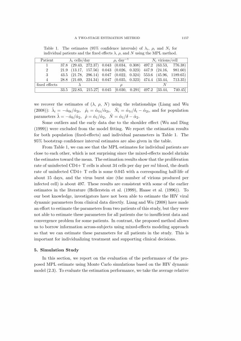
Table 1. The estimates (95% confidence intervals) of λi, ρi and Ni forindividual patients and the fixed effects λ, ρ, and N using the MPL method.
Patient λi cells/day ρi day−1 Ni virions/cell1 37.8 (29.43, 272.37) 0.043 (0.034, 0.308) 497.2 (63.53, 776.38)2 21.9 (13.17, 157.56) 0.043 (0.026, 0.323) 447.9 (24.16, 981.60)3 43.5 (21.78, 296.14) 0.047 (0.022, 0.324) 553.6 (45.96, 1189.65)4 28.8 (21.69, 224.34) 0.047 (0.035, 0.323) 474.4 (33.44, 713.35)
fixed effects λ ρ N33.5 [22.83, 215.27] 0.045 [0.030, 0.291] 497.2 [33.44, 740.45]
we recover the estimates of (λ, ρ, N) using the relationships (Liang and Wu(2008)): λi = −α0i/α2i, ρi = α1i/α2i, Ni = α1i/δi − α2i, and for populationparameters λ = −α0/α2, ρ = α1/α2, N = α1/δ − α2.
Some outliers and the early data due to the shoulder effect (Wu and Ding(1999)) were excluded from the model fitting. We report the estimation resultsfor both population (fixed-effects) and individual parameters in Table 1. The95% bootstrap confidence interval estimates are also given in the table.
From Table 1, we can see that the MPL estimates for individual patients areclose to each other, which is not surprising since the mixed-effects model shrinksthe estimates toward the mean. The estimation results show that the proliferationrate of uninfected CD4+ T cells is about 34 cells per day per ml blood, the deathrate of uninfected CD4+ T cells is some 0.045 with a corresponding half-life ofabout 15 days, and the virus burst size (the number of virions produced perinfected cell) is about 497. These results are consistent with some of the earlierestimates in the literature (Hellerstein et al. (1999), Haase et al. (1996)). Toour best knowledge, investigators have not been able to estimate the HIV viraldynamic parameters from clinical data directly. Liang and Wu (2008) have madean effort to estimate the parameters from two patients of this study, but they werenot able to estimate these parameters for all patients due to insufficient data andconvergence problem for some patients. In contrast, the proposed method allowsus to borrow information across-subjects using mixed-effects modeling approachso that we can estimate these parameters for all patients in the study. This isimportant for individualizing treatment and supporting clinical decisions.
5. Simulation Study
In this section, we report on the evaluation of the performance of the pro-posed MPL estimate using Monte Carlo simulations based on the HIV dynamicmodel (2.3). To evaluate the estimation performance, we take the average relative

1158 YUN FANG, HULIN WU AND LI-XING ZHU
Table 2. The AREs (%) of the MPL estimates for individual parametersα0i, α1i, α2i and fixed effects α0, α1, α2 for the first simulation scheme inSection 5. (n = 4, ni = 36).
γ∗1 γ∗
2 α0i α1i α2i α0 α1 α2
100 10 5.68 34.17 22.93 4.81 32.17 22.84400 10 5.61 34.12 22.99 4.89 32.73 22.89100 20 6.37 35.22 22.36 5.74 34.43 22.62400 20 6.30 35.18 22.42 5.67 34.80 22.32
estimation error (ARE) of θ as
ARE =1
Ns
Ns∑i=1
|θ − θ||θ|
× 100%,
where θ is the estimate of θ and Ns is the number of simulation runs. Twosimulation schemes were designed as suggested by the referee.
Simulation Scheme 1. To get the performance of the proposed MPLestimate in the application in Section 4, the first simulation experiment mimicsthe study. We used the estimated parameters and the estimated initial valuesVi(0) and Ti(0) for individual subjects in Section 4 to generate data. Since we canonly estimate Ti(0), we assumed that the ratio of TUi(0) and TIi(0) is 1 : 10 toobtain the initial values for TUi(0) and TIi(0). The time varying infection rate η(t)of T cells was set at 9×10⁻⁵(1−0.9 cos(πt/100)). The measurement errors ε1i(t)and ε2i(t) were independently generated from normal distributions with meanszero and variances γε1(t, t) = 400 and 100 and γε2(t, t) = 20 and 10, respectively.We generated our data by numerically solving the ODE system (2.1) via thefourth-order Runge-Kutta algorithm, and then measurement errors were addedto the simulated data Vi(t) and Ti(t). For simplicity, we took 36 measurements foreach of the four patients as designed by this application study. We simulated 500data sets and applied the proposed MPL estimation method to these simulateddata sets. Note that the Epanechnikov kernel K(u) = (3/4)(1 − u2)I(|u| ≤ 1)and the bandwidth selection method proposed in Section 2.1 were used in theestimation. The fixed-effect parameters α0, α1, α2 and the individual parametersα0i, α1i, α2i in (4.2) were estimated and their ARE’s are reported in Table 2.
From Table 2, we can see that the AREs of the MPL estimates for fixedeffects and individual parameters, ranging from 5% to 35%, are quite reasonable.This suggests that our estimates of these kinetic parameters for these patientsare reliable.
Simulation Scheme 2. To further illustrate the performance for differentsample sizes, we designed the second simulation scheme as follows. First we

A TWO-STAGE ESTIMATION METHOD 1159
chose the fixed-effect parameters as (α0, α1, α2) = (45,918, -138, -1,276), thenthe random effects of parameters (b0i, b1i, b2i) were generated independently froma multivariate normal distribution with mean 0 and variance diag(104, 4, 36),based on the data analysis results in Section 4. Thus the parameters α0i, α1i,α2i, and ci for individual subjects in model (2.3) were obtained by adding thefixed effects and random effects, together as in (4.2) . Secondly, we calculatedthe parameters λi, ρi, and Ni for the i-th individual in original ODE model(2.1) based on their relationships with α0i, α1i, α2i and ci (see Section 4). Thefixed effects of initial values for the state variables (TU (0), TI(0), V (0)) were setas (30, 600, 105). The random effects of initial values (bUi(0), bIi(0), bV i(0)) wereindependently generated from a multivariate normal distribution with mean 0and variance diag(4, 40, 106). The time-varying infection rate of T cells for eachindividual was ηi(t) = 9×10⁻⁵(1−0.9 cos(πt/1, 000)). The death rate of infectedCD4+ T cells is fixed as δi = 0.5/day and the clearance rate of virus is fixed asci = 3 based on the estimates from the literature (Perelson et al. (1996)). Themeasurement errors ε1i(t) and ε2i(t) are independently generated from normaldistributions with means zero and variances γε1(t, t) = γ∗
1 [1 + 0.75 cos(t/40)] andγε2(t, t) = γ∗
1 [1+0.1 sin(t/80)] with γ∗1 = (50, 200) and γ∗
2 = (10, 40), respectively.Finally, we simulated our data by numerically solving the ODE system (2.1) viathe fourth-order Runge-Kutta algorithm, and then the measurement errors wereadded to the simulated data Vi(t) and Ti(t).
We chose three different sample sizes for the simulated data: a) n = 8,ni = 30+Poisson(8); b) n = 8, ni = 60+Poisson(16); and c) n = 16, ni =30+Poisson(8), where a Poisson distribution was used to mimic the unbalanceddata for individual subjects. The observation time points were equally-spacedfor simplicity: tij = 0.1 × j with j = 1, 2, . . . , ni. We carried out Ns = 500 sim-ulation runs. Similarly, we used the proposed MPL to estimate the fixed-effectparameters (α0, α1, α2) and individual parameters (α0i, α1i, α2i). We report theARE’s of these estimates in Table 3. From Table 3, we can see that the overallperformance for both population parameter estimates and individual parame-ter estimates were reasonably good for the proposed MPL method. For largersample sizes, the performance of the estimator of fixed effects was better. Also,with ni larger, the ARE’s of the MPL estimator for both fixed and individualparameters are smaller, which suggests the importance of the sample size forindividual subjects for the proposed method, since it is necessary to obtain goodnonparametric estimates for the state variables in the first stage. The ARE’sof individual parameter estimates are generally larger than those of fixed effectsestimates, as expected. Additional simulations were performed for the data with
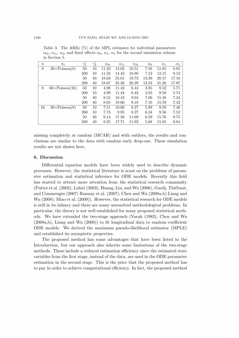
1160 YUN FANG, HULIN WU AND LI-XING ZHU
Table 3. The AREs (%) of the MPL estimates for individual parametersα0i, α1i, α2i and fixed effects α0, α1, α2 for the second simulation schemein Section 5.
n ni γ∗1 γ∗
2 α0i α1i α2i α0 α1 α2
8 30+Poisson(8) 50 10 11.23 14.03 10.51 7.56 11.85 8.85200 10 11.33 14.43 10.80 7.53 12.15 9.1250 40 18.63 25.01 19.73 13.39 20.57 17.10200 40 18.67 25.26 20.29 13.53 21.26 17.97
8 60+Poisson(16) 50 10 4.98 11.43 6.44 3.85 9.52 5.71200 10 4.99 11.44 6.43 3.83 9.58 5.7450 40 8.55 18.43 9.04 7.06 15.48 7.34200 40 8.65 18.66 9.18 7.16 15.59 7.42
16 30+Poisson(8) 50 10 7.51 10.00 8.27 5.99 9.59 7.46200 10 7.73 9.95 8.27 6.34 9.56 7.5250 40 9.14 17.38 11.69 6.59 15.76 9.75200 40 9.25 17.71 11.93 5.68 15.85 9.64
missing completely at random (MCAR) and with outliers, the results and con-clusions are similar to the data with random early drop-out. These simulationresults are not shown here.
6. Discussion
Differential equation models have been widely used to describe dynamicprocesses. However, the statistical literature is scant on the problems of param-eter estimation and statistical inference for ODE models. Recently this fieldhas started to attract more attention from the statistical research community(Putter et al. (2002), Lahiri (2003), Huang, Liu, and Wu (2006), Guedj, Thiebaut,and Commenges (2007) Ramsay et al. (2007), Chen and Wu (2008a,b) Liang andWu (2008); Miao et al. (2009)). However, the statistical research for ODE modelsis still in its infancy and there are many unresolved methodological problems. Inparticular, the theory is not well established for many proposed statistical meth-ods. We have extended the two-stage approach (Varah (1982), Chen and Wu(2008a,b), Liang and Wu (2008)) to fit longitudinal data to random coefficientODE models. We derived the maximum pseudo-likelihood estimator (MPLE)and established its asymptotic properties.
The proposed method has some advantages that have been listed in theIntroduction, but our approach also inherits some limitations of the two-stagemethods. These include a reduced estimation efficiency since the estimated statevariables from the first stage, instead of the data, are used in the ODE parameterestimation in the second stage. This is the price that the proposed method hasto pay in order to achieve computational efficiency. In fact, the proposed method

A TWO-STAGE ESTIMATION METHOD 1161
can be combined with the exact maximum likelihood approach (Guedj, Thiebaut,and Commenges (2007)) to improve the estimation efficiency, which is a worthytopic for future research.
We have worked under the assumption that the second stage parametricmodel is linear in unknown parameters so that the linear mixed-effects (LME)model can be used. However, the proposed estimation procedure is applicable toa general nonlinear model in the second stage. In this case, however, the nonlin-ear mixed-effects model (Davidian and Giltinan (1993), Davidian and Giltinan(1995), Vonesh and Chinchilli (1996)) instead of LME model, should be fitted inthe second stage. The theoretical development is also more tedious in the nonlin-ear model case. We considered a single ODE model for notational simplicity andcomputational convenience, but our method can be generalized to multivariateODE models. It is still an open question how to use the two-stage approachto deal with latent (unmeasurable) state variables. In this paper, we employedthe local polynomial nonparametric approach in the first stage. In fact, manyother nonparametric smoothing methods such as regression splines, smoothingsplines, and penalized splines (Wu and Zhang (2006)) can be used to fit the non-parametric mixed-effects model in the first stage. Also note that the standardregression estimation for each individual subject, instead of a mixed-effects re-gression model, can be used to estimate the unknown parameters in the secondstage, though this may fail if the data from some individual subjects are toosparse. Our methodological development is motivated by HIV dynamic studies,but we also expect that our method can be applied to other ODE models withlongitudinal data.
Acknowledgement
Fang was supported by a NSF grant from the National Natural ScienceFoundation of China (No. 10701035), ChenGuang project of Shanghai Educa-tion Development Foundation (No. 2007CG33); Wu was partially supported byUSA NIH grants AI055290, AI50020, AI078498, AI078842, and AI087135; andZhu was supported by a grant (HKU 2030/07P) from the Research Grants Coun-cil of Hong Kong and a FRG grant from Hong Kong Baptist University, HongKong. This paper was completed while the first author was visiting the Depart-ment of Biostatistics & Computational Biology, University of Rochester Schoolof Medicine and Dentistry as a visiting PhD student under the supervision of thesecond author and she appreciates the hospitality and support from the Depart-ment. The authors are also grateful to Drs. Hua Liang and Hongqi Xue for theirhelpful discussions on the proofs of the theoretical results. The authors thank anAE and a referee for their constructive comments and suggestions.

1162 YUN FANG, HULIN WU AND LI-XING ZHU
Appendix
Proof of Lemma 2.1. For estimating the derivatives u′(t) and v′i(t), a localquadratic (p = 2) linear mixed-effects (LME) model is used, i.e.,
Gi =
si,0 si,1 si,2
si,1 si,2 si,3
si,2 si,3 si,4
=f(t)σ2(t)
ni 0 nih2B(K)
0 nih2B(K) 0
nih2B(K) 0 nih
4E(K)
×[1 + Op((nih)−1/2)]. (A.1)
Since (C9), D = diag(d21(t), d
22(t), d
23(t)), it follows that
G−1i D−1 =
σ2(t)f(t)
E(K)d2
1(t)ni(E(K)−B2(K))
0 nih2B(K)
0 d22(t)
nih2B(K)0
nih2B(K) 0 d2
3(t)nih4(E(K)−B2(K))
×[1 + Op((nih)−1/2)]. (A.2)
When different bandwidths, h11 and h12, are used to estimate u′(t) and v′i(t), theh in (A.1) and (A.2) can be replaced by h11 and h12. We prove the lemma in thefollowing three steps.Step 1. By the proof of Theorem 1 in Wu and Zhang (2002), we have
eτ2{
n∑k=1
(I + GkD)−1G−1k }−1 × (I + GiD)−1Gi =
1n
[1 + Op(n−1i )]eτ
2 . (A.3)
Recall the expression for u(t) in (2.15). We have
u′(t) − u′(t)
=:
{n−1
n∑i=1
ni∑j=1
eτ2G
−1i Hij,2(t)
Kh,11(tij − t)σ2(t)
×[u(tij) − u(t) − (tij − t)u′(t) − (tij − t)2
2u(2)(t)
]+n−1
n∑i=1
ni∑j=1
eτ2G
−1i Hij,2(t)
Kh,11(tij − t)σ2(t)
[vi(tij) + ei(tij)]
}[1 + op(1)]
=:
[h2
11u(3)(t)E(K)3!B(K)
+ n−1n∑
i=1
ξ1i(t)
][1 + op(1)]. (A.4)
The {ξ1i(t), i = 1, . . . , n} are independent. Here Hij,2(t) = (1, (tij − t), (tij − t)2)τ
and Kh,11(·) = h−111 K(·/h11).

A TWO-STAGE ESTIMATION METHOD 1163
Step 2. By the proof of Theorem 1 in Wu and Zhang (2002), we have eτ2D(I +
GiD)−1Gi = eτ2 + op(1). Then, based on v′(t) given in (2.15) in Section 2, we
obtain that
v′i(t) =ni∑
j=1
eτ2G
−1i Hij,2(t)
Kh,12(tij − t)σ2(tij)
×
{Yij − Hτ
ij,2(t)1n
n∑i=1
ni∑l=1
eτ2G
−1i Hij,2(t)
Kh,12(til − t)σ2(til)
Yij
}
=
{ni∑
j=1
eτ2G
−1i Hij,2(t)
Kh,12(tij − t)σ2(tij)
[vi(tij) + ei(tij)]
−n−1n∑
i=1
ni∑j=1
eτ2G
−1i Hij,2(t)
Kh,12(tij − t)σ2(t)
[vi(tij)+ei(tij)]
}[1+Op(m−1)]
=:[ξ2i(t) −
1n
n∑i=1
ξ2i(t)][1 + op(1)].
Step 3. In summary,
∆i(t) =
[h2
11u(3)(t)E(K)3!B(K)
+ξ2i(t)−v′i(t)+n−1n∑
i=1
ξ1i(t) −1n
n∑i=1
ξ2i(t)
][1+op(1)],
where {ξ1i(t), i = 1, . . . , n} and {ξ2i(t), i = 1, . . . , n} are series of i.i.d. randomvariables with mean 0. We have
Var (ξ2i(t)|D) = d22(t) +
τ2(t)C(K)nih3
12B2(K)f(t)
+ op[(nih312)
−1]. (A.5)
Consequently, Var (n−1∑n
i=1 ξ2i(t)−n−1∑n
i=1 ξ2i(t)|D) = Op[(nnih3)−1]. Under
(C7), similarly, n−1∑n
i=1 ξ2i(t) − n−1∑n
i=1 ξ2i(t) = Op[(nnih3)−1/2]. On the
other hand,
Var (ξ2i(t) − v′i(t|D) =τ2(t)C(K)
nih312B
2(K)f(t)+ op[(nih
312)
−1/2]. (A.6)
Therefore, by (C7), n−1∑n
i=1 ξ1i(t) − n−1∑n
i=1 ξ2i(t) is of higher order thanξ2i(t) − v′i(t). Finally,
∆i(t) =h2
11u(3)(t)E(K)3!B(K)
+ ξ2i(t) − v′i(t) + op[h211 + (nih
312)
−1/2], (A.7)

1164 YUN FANG, HULIN WU AND LI-XING ZHU
By (A.7) and (A.6), we conclude that
E[∆i(t)|D] =h2
11u(3)(t)E(K)3!B(K)
+ op(h211),
Var [∆i(t)|D] =τ2(t)C(K)
nih312B
2(K)f(t)+ op[(nih
312)
−1/2].(A.8)
This completes the proof of Lemma 2.1.
Proof of Lemma 2.2. By (A.7) in the proof of Lemma 2.1, it is easy to de-rive that Cov(∆i(t1),∆j(t2)|D) = op[(nih
312)
−1]. Let µ(t) = (3!B(K)−1)h211E(K)
u(3)(t). Note that ∆i(t1) and ∆j(t2) are normal vectors. Thus(√nih3
12[∆i(t1) − µ(t1)],√
njh312[∆j(t2) − µ(t2)]|D
)d−→ N
(0,
C(K)B2(K)
diag
(τ2(t1)f(t1)
,τ2(t2)f(t2)
)).
By Definition 2.1, under the design D, ∆i(t1) and ∆j(t2) are asymptoticallyindependent for i 6= j. Then it is obvious that the vectors ∆i and ∆j areasymptotically conditionally independent.
Proof of Lemma 3.1. Let Hij,1(t) = (1, tij − t)τ . Similar to proof of Lemma2.1, we have
Λi(t) =
{1n
n∑i=1
ni∑j=1
eτ2G
−1i Hij,1(t)
Kh,01(tij − t)σ2(t)
[u(tij) − u(t) − (tij − t)u′(t)
]
+ξ3i(t) − vi(t)
}[1 + op(1)]
=
[h2
01u(2)(t)B(K)
2+ ξ3i(t) − vi(t)
][1 + op(1)],
where
ξ3i(t) =ni∑
j=1
eτ1G
−1i Hij,1(t)
Kh,02(tij − t)σ2(tij)
[vi(tij) + ei(tij)].
Obviously E(ξ3i(t)|D) = 0, and the conditional variance of ξ3i(t) is
Var (ξ3i(t) − vi(t)|D) =τ2(t)V (K)nih02f(t)
+ op[(nih02)−1].
So in summary, we find
E(Λi(t)|D) =h2
01u(2)(t)B(K)
2+ op(h2
01),

A TWO-STAGE ESTIMATION METHOD 1165
V ar(Λi(t)|D) =τ2(t)V (K)nih02f(t)
+ op[(nih02)−1].
The proof of Lemma 3.1 is completed.
Proof of Theorem 3.1. Note that θ = [∑n
i=1 Fτi V
−1i Fi]−1[
∑ni=1 Fτ
i V−1i X′
i] in(2.27), where Fi = (F (Xi(ti1)), . . . , F (Xi(tini)))
τ , Vi = FiDθFτi + Ri. First, for
the matrix, V−1i , we have
V−1i = R−1
i − R−1i Fi(D−1
θ + Fτi R
−1i Fi)−1Fτ
i R−1i . (A.9)
Then
Fτi V
−1i Fi
= Fτi R
−1i Fi − Fτ
i R−1i Fi
{D−1
θ + Fτi R
−1i Fi
}−1Fτ
i R−1i Fi
= Fτi R
−1i Fi − (Fτ
i R−1i Fi)1/2
×{
(Fτi R
−1i Fi)−1/2D
−1/2θ D
−1/2θ (Fτ
i R−1i Fi)−1/2 + I
}−1(Fτ
i R−1i Fi)1/2,(A.10)
and furthermore,{(Fτ
i R−1i Fi)−1/2D
−1/2θ D
−1/2θ (Fτ
i R−1i Fi)−1/2 + I
}−1
= I − (Fτi R
−1i Fi)−1/2D
−1/2θ
[I + D
−1/2θ (Fτ
i R−1i Fi)−1D
−1/2θ
]−1
×D−1/2θ (Fτ
i R−1i Fi)−1/2. (A.11)
Substitute (A.11) into (A.10). Note that Ri is the variance-covariance matrix of∆i and each element of Ri is op(1). F is a ni × q matrix. So each element of(Fτ
i R−1i Fi)−1 goes to +∞ as ni → +∞. With (Fτ
i R−1i Fi)−1 = op(1), we have
Fτi V
−1i Fi = D
−1/2θ
[I + D
−1/2θ (Fτ
i R−1i Fi)−1D
−1/2θ
]−1D
−1/2θ
= D−1/2θ [I + op(1)]−1D
−1/2θ = D−1
θ + op(1). (A.12)
Similarly, Fτi V
−1i Fi = D−1
θ + op(1). So we have∑n
i=1 Fτi V
−1i Fi = nD−1
θ + op(n).For notation simplicity, we use bi to represent the random component of θi.Moreover, we have
n∑i=1
Fτi V
−1i X′
i =∑i=1
Fτi V
−1i [Fiθ + Fibi + ∆i]
= [nD−1θ θ + D−1
θ
n∑i=1
bi +n∑
i=1
Fτi V
−1i ∆i][1 + op(1)].

1166 YUN FANG, HULIN WU AND LI-XING ZHU
Consequently, it is obvious that
θ ={D−1
θ + op(1)}−1
×
{D−1
θ θ + D−1θ
1n
n∑i=1
bi +1n
n∑i=1
Fτi V
−1i ∆i
}[1 + op(1)]. (A.13)
By a similar procedure from (A.10) to (A.12),
1n
n∑i=1
Fτi V
−1i ∆i =
1n
n∑i=1
D−1θ (FiR−1
i Fi)−1FiR−1i ∆i[1 + op(1)].
By Lemma 2.1, E(∆i|D) = Op(h212), one has
E(1n
n∑i=1
D−1θ (FiR−1
i Fi)−1FiR−1i ∆i|D) = Op(h2
12). (A.14)
By Lemma 2.2, ∆i and ∆j are asymptotically independent. Since (Fτi R
−1i Fi)−1
= op(1),
V ar( 1
n
n∑i=1
D−1θ (Fτ
i R−1i Fi)−1Fτ
i R−1i ∆i|D
)=
1n2
n∑i=1
D−1θ (Fτ
i R−1i Fi)−1D−1
θ
= op(n−1). (A.15)
Then based on (A.14) and (A.15),
1n
n∑i=1
Fτi V
−1i ∆i = Op(h2
11) + op(n−1/2). (A.16)
On the other hand, n−1∑n
i=1 bi = Op(n−1/2). Then by (A.13), θ = θ + op(1),and θ is a consistent estimator of θ.
Proof of Theorem 3.2. First, we can rewrite θ = [n−1∑n
i=1 Fτi V
−1i Fi]−1
[n−1∑n
i=1 Fτi V
−1i X′
i]. By (A.12), we have
θ − θ (A.17)
= [n−1n∑
i=1
Fτi V
−1i Fi]−1[n−1
n∑i=1
Fτi V
−1i X′
i − n−1n∑
i=1
Fτi V
−1i Fiθ]
= [D−1θ + op(1)]−1[n−1
n∑i=1
Fτi V
−1i (Fi − Fi)θ + n−1
n∑i=1
Fτi V
−1i ∆i
+n−1n∑
i=1
Fτi V
−1i Fibi]

A TWO-STAGE ESTIMATION METHOD 1167
= n−1n∑
i=1
bi + op(n−1/2) + Dθ
[1n
n∑i=1
Fτi V
−1i ∆i −
1n
n∑i=1
FiV−1i ΛiF∗′
i θ
]×[1 + op(1)], (A.18)
where F∗i = (F (Xi(ti1) + φi1 ∗ Λi(ti1)), . . . , F (Xi(tini) + φini ∗ Λi(tini)))
τ , F∗′i
denotes the derivative of F∗i , and {φi1, . . . , φini} is a series of numbers between
0 and 1. Λi = diag(Λi(ti1)), . . . , Λi(tini))). Then by (A.16), we can obtain that
1n
n∑i=1
DθFτi V
−1i ∆i = Op(h2
11) + op(n−1/2).
Similarly, we find
1n
n∑i=1
DθFiV−1i ΛiF∗′
i θ = Op(h201) + op(n−1/2).
Under condition (C8), h01 = op(n−1/4), h11 = op(n−1/4), so
1n
n∑i=1
DθFτi V
−1i ∆i = op(n−1/2),
1n
n∑i=1
DθFiV−1i ΛiF∗′
i θ = op(n−1/2).
Thus, under (C8) and based on (A.18), we represent θ − θ as
θ − θ =1n
n∑i=1
bi + op(n−1/2).
It is assumed that {bi, i = 1, . . . , n} are i.i.d. random vectors with mean 0 andvariance matrix Dθ. By Central Limit Theorem, we get
√n(θ−θ) d−→ N(0, Dθ),
the conclusion of Theorem 3.2.
References
Besag, J. (1974). Spatial interaction and the statistical analysis of lattice systems. J. Roy.
Statist. Soc. Ser. B 36, 192-236.
Besag, J. (1977). Efficiency of pseudolikelihood estimation for simple Gaussian fields.
Biometrika 64, 616-618.
Brunel, N. (2008). Parameter estimation of ODE’s via nonparametric estimators. Electronic J.
Statist. 2, 1242-1267.
Carroll, R. J., Fan, J., Gijbels, I. and Wand, M. P. (1997). Generalized partially linear single-
index models. J. Amer. Statist. Assoc. 92, 477-489.
Chen, J. and Wu, H. (2008a). Efficient local estimation for time-varying coefficients in deter-
ministic dynamic models with applications to HIV-1 dynamics. J. Amer. Statist. Assoc.
103, 369-384.

1168 YUN FANG, HULIN WU AND LI-XING ZHU
Chen, J. and Wu, H. (2008b). Estimation of time-varying parameters in deterministic dynamic
models. Statist. Sinica 18, 987-1006.
Davidian, M. and Giltinan, D. M. (1993). Some general estimation methods for nonlinear mixed
effects models. J. Biopharmaceutical Statist. 3, 23-55.
Davidian, M. and Giltinan, D. M. (1995). Nonlinear Models for Repeated Measurement Data.
Chapman & Hall, London.
Draisma, G., Dree, H., Ferreira, A. and Hann, L. D. (2004). Bivariate tail estimation: depen-
dence in asymptotic independence. Bernoulli 10, 251-280.
Ellner, S., Seifu, Y. and Smith, R. H. (2002). Fitting population dynamic models to time-series
data by gradient matching. Ecology 83, 2256-2270.
Gong, G. and Samaniego, F. J. (1981). Pseudo maximum likelihood estimation: theory and
application. Ann. Statist. 9, 861-869.
Guedj, J., Thiebaut, R. and Commenges, D.(2007). Maximum likelihood estimation in dynam-
ical models of HIV. Biometrics 63, 1198-1206.
Haase, A. T., Henry, K., Zupancic, M., Sedgewick, G., Faust, R. A., Melroe, H., Cavert, W.,
Gebhard, K., Staskus, K., Zhang, Z.-Q., Dailey, P. J., Balfour Jr., H. H., Erice, A. and
Perelson, A. S. (1996). Quantitative image analysis of HIV-1 infection in lymphoid tissue.
Science 274, 985-989.
Hart, J. D. and Wehrly, T. E. (1993). Consistency of cross-validation when the data are curves.
Stochastic Process. Appl. 45, 351-361.
Hellerstein, M., Hanley, M. B., Cesar, D., Siler, S., Papageorgopoulos, C., Wieder, E., Schmidt,
D., Hoh, R., Neese, R., Macallan, D., Deeks, S. and McCune, J. M. (1999). Directly
measured kinetics of circulating T lymphocytes in normal and HIV-1-infected humans.
Nature Medicine 5, 83-89.
Ho, D. D., Neumann, A. U., Perelson, A. S., Chen, W., Leonard, J. M. and Markowitz, M.
(1995). Rapid turnover of plasma virions and CD4 lymphocytes in HIV-1 infection. Nature
373, 123-126.
Huang, Y., Liu, D. and Wu, H. (2006). Hierarchical Bayesian methods for estimation of param-
eters in a longitudinal HIV dynamic system. Biometrics 62, 413-423.
Huang, Y. and Wu, H. (2006). A Bayesian approach for estimating antiviral efficacy in HIV
dynamic models. J. Appl. Statist. 33, 155-174.
Hurlimann, W. (2004). On the rate of convergence to asymptotic independence between order
statistics. Statist. Probab. Lett. 66, 355-362.
Lahiri, S. N. (2003). A necessary and sufficient condition for asymptotic independence of discrete
fourier transforms under short-and long-range dependence. Ann. Statist. 31, 613-641.
Liang, H., Wu, H. and Carroll, R.J. (2003). The relationship between virologic and immunologic
responses in AIDS clinical research using mixed-effects varying-coefficient semiparametric
models with Measurement Error. Biostatistics 4, 297-312.
Liang, H. and Wu, H. (2008). Parameter estimation for differential equation models using a
framework of measurement error in regression. J. Amer. Statist. Assoc. 103, 1570-1583.
Miao, H., Dykes, C., Demeter, L. M. and Wu, H. (2009). Differential equation modeling of HIV
viral fitness experiments: model identification, model Selection, and multi-model inference.
Biometrics 65, 292-300.
Nowak, M. A. and May, W. H. (2000). Virus Dynamics: Mathematical Principles of Immunology
and Virology. Oxford University Press, Oxford.

A TWO-STAGE ESTIMATION METHOD 1169
Perelson, A. S., Essunger, P., Cao, Y. Z., Vesanen, M., Hurley, A., Saksela, K., Markowitz,
M. and Ho, D. D. (1997). Decay characteristics of HIV-1-infected compartments during
combination therapy. Nature 387, 181-191.
Perelson, A. S., Neumann, A. U., Markowitz, M., Leonard, J. M. and Ho, D. D. (1996). HIV-1
dynamics in vivo: virion clearance rate, infected cell life-span, and viral generation time.
Science 271, 1582-1586.
Perelson, A. S. and Nelson, P. W. (1999). Mathematical analysis of HIV-1 dynamics in vivo.
SIAM Rev. 41, 3-44.
Putter, H., Heisterkamp, S. H., Lange, J. M. and De Wolf, F. (2002). A Bayesian approach to
parameter estimation in HIV dynamical models. Stat. Med. 21, 2199-2214.
Ramsay, J. O., Hooker, G., Campbell, D. and Cao, J. (2007). Parameter estimation for differ-
ential equations: a generalized smoothing approach (with discussion). J. Roy. Statist. Soc.
Ser. B 69, 741-796.
Rice, J. A. and Silverman, B. W. (1991). Estimating the mean and covariance structure non-
parametrically when the data are curves. J. Roy. Statist. Soc. Ser. B 53, 233-243.
Rice, J. A. and Wu, C. O. (2001). Nonparametric mixed effects models for unequally sampled
noisy curves. Biometrics 57, 253-259.
Shi, M., Weiss, R. E. and Taylor, J. M. (1996). An analysis of pediatric CD4 counts for acquired
immune deficiency syndrome using flexible random curves. Appl. Statist. 45, 151-163.
Stute, W. and Zhu, L. X. (2005). Nonparametric checks for single-index models. Ann. Statist.
33, 1048-1083.
Tan, W. Y. and Wu, H. (2005). Deterministic and Stochastic Models of AIDS Epidemics and
HIV Infections with Intervention. World Scientific, Singapore.
Troxel, A. B., Lipsitz, T. R. and Harrington, D. P. (1998). Marginal models for the analysis of
longitudinal measurements with nonignorable non-monotone missing data. Biometrika 85,
661-672.
Varah, J. M. (1982). A spline least squares method for numerical parameter estimation in
differential equations. SIAM J. Sci. Comput. 3, 28-46.
Vonesh, E. F. and Chinchilli, V. M. (1996). Linear and Nonlinear Models for the Analysis of
Repeated Measurements. Marcel Dekker, New York.
Wu, H. (2005). Statistical methods for HIV dynamic studies in AIDS clinical trials. Statist.
Meth. Medical Res. 14, 171-192.
Wu, H. and Ding, A. (1999). Population HIV-1 dynamics in vivo: applicable models and infer-
ential tools for virological data from AIDS clinical trials. Biometrics 55, 410-418.
Wu, H. and Liang, H. (2004). Backfitting random varying-coefficient models with time-
dependent smoothing covariates. Scan. J. Statist. 31, 3-19.
Wu, H., Kuritzkes, D. R., McClernon, D. R., Kessler, H., Connick, E., Landay, A., Spear, G.,
Heath-Chiozzi, M., Rousseau, F., Fox, L., Spritzler, J., Leonard, J. M. and Lederman,
M. M. (1999). Characterization of viral dynamics in human immunodeficiency virus type
1-infected patients treated with combination antiretroviral therapy: Relationships to host
factors, cellular restoration, and virologic end points. J. Infectious Diseases 179, 799-807.
Wu, H. and Zhang, J. T. (2002). Local polynomial mixed-effects models for longitudinal data.
J. Amer. Statist. Assoc. 97, 883-897.
Wu, H. and Zhang, J. T. (2006). Nonparametric regression methods for longitudinal data anal-
ysis. Wiley, New Jersey.

1170 YUN FANG, HULIN WU AND LI-XING ZHU
Mathematics and Science College, Shanghai Normal University, Shanghai, China.
E-mail: [email protected]
Department of Biostatistics and Computational Biology, University of Rochester School of
Medicine and Dentistry, Rochester, NY 14642 , U.S.A.
E-mail: [email protected]
Department of Biostatistics and Department of Mathematics, Hong Kong Baptist University,
HK, China.
E-mail: [email protected]
(Received June 2009; accepted March 2010)