lable at ScienceDirect

Environmental Modelling & Software 62 (2014) 1e15

Contents lists avai

Environmental Modelling & Software

journal homepage: www.elsevier .com/locate/envsoft

A tightly coupled GIS and distributed hydrologic modeling framework

Gopal Bhatt*, Mukesh Kumar, Christopher J. DuffyDepartment of Civil and Environmental Engineering, The Pennsylvania State University, 212 Sackett Building, University Park, PA 16802, USA

a r t i c l e i n f o

Article history:Received 1 September 2013Received in revised form4 August 2014Accepted 5 August 2014Available online xxx

Keywords:Distributed hydrologic modelGISPIHMPIHMgisShared geodata model

* Corresponding author.E-mail address: gopal.bhatt@psu.edu (G. Bhatt).

http://dx.doi.org/10.1016/j.envsoft.2014.08.0031364-8152/© 2014 Elsevier Ltd. All rights reserved.

a b s t r a c t

Distributed, physics-based hydrologic models require spatially explicit specification of parametersrelated to climate, geology, land-cover, soil, and topography. Extracting these parameters from nationalgeodatabases requires intensive data processing. Furthermore, mapping these parameters to model meshelements necessitates development of data access tools that can handle both spatial and temporaldatasets. This paper presents an open-source, platform independent, tightly coupled GIS and distributedhydrologic modeling framework, PIHMgis (www.pihm.psu.edu), to improve model-data integration.Tight coupling is achieved through the development of an integrated user interface with an underlyingshared geodata model, which improves data flow between the PIHMgis data processing components. Thecapability and effectiveness of the PIHMgis framework in providing functionalities for watersheddelineation, domain decomposition, parameter assignment, simulation, visualization and analyses, isdemonstrated through prototyping of a model simulation. The framework and the approach are appli-cable for watersheds of varied sizes, and offer a template for future GIS-Model integration efforts.

© 2014 Elsevier Ltd. All rights reserved.

Software availability

PIHMgisDevelopers: Gopal Bhatt, Mukesh KumarContact Address: Department of Civil & Environmental

Engineering, 212 Sackett Building, University Park, PA16802, USA

Email: gopal.bhatt@psu.edu, mukesh.kumar@duke.eduYear First Available: 2006Hardware Required: Desktop/Laptop with 2 GHz CPU, 2 GB RAM or

moreOperating System Required: Macintosh OSX 10.4 or newer;

Windows XP or newer; LinuxLibraries Required: SUNDIALS, Qt4, GDAL, SQLite, GEOS, GSL, Expat,

and PostgreSQLAvailability: http://www.pihm.psu.eduCost: FreeSource Code: http://sourceforge.net/projects/pihmgis/Program Language: C/Cþþ

1. Introduction

Physics based, fully coupled distributed hydrologic models suchas FIHM/PIHM3D (Kumar et al., 2009a), InHM (VanderKwaak,

1999), MIKE-SHE (Abbott et al., 1986a,b; DHI, 2005), MODFLOW-SURFACT (McDonald and Harbaugh, 1988; Panday and Huyakorn,2008), ParFlow (Kollet and Maxwell, 2006), Penn State IntegratedHydrologic Model (PIHM) (Qu and Duffy, 2007; Kumar 2009),PREVAH (Viviroli et al., 2009), WASH123D (Yeh and Huang, 2003),and WATFLOOD (Kouwen, 1988), simulate spatially explicit hydro-logic response. These models also capture the heterogeneities inhydrogeologic and meteorological parameters within the water-shed at finer spatial resolutions (Freeze and Harlan, 1969; Clark,1998; Singh and Fiorentino, 1996; Entekhabi and Eagleson, 1989;Haverkamp et al., 2005; Pitman et al., 1990; Kollet and Maxwell,2006; Kumar et al., 2009b), and have been demonstrated toenhance understanding and prediction of hydrologic processes(Refsgaard, 1997; Boyle et al., 2003; Meixner et al., 2003; Kirchner,2006; Shrestha and Rode, 2008; Lu et al., 2009; Kumar et al., 2013).One of the key challenges in application of distributed, physicsbased models is the lack of a framework for efficient prototyping ofmodel simulations, evaluation of a-priori parameters, and forsimulation, analysis and visualization (Goodchild, 1992; DeVantierand Feldman, 1993; Nyerges, 1993; McDonnell, 1996; Moore, 1996;Sui and Maggio, 1999; Duffy et al., 2011).

Distributed hydrologic models require assignment of watershedparameters related to geology, soil, topography, land use, landcover, initial conditions, precipitation, and meteorological condi-tions, to all mesh elements within the model domain. Because ofthe inherent heterogeneity in geospatial data sets, the process ofassigning parameters to large number of mesh elements is an error

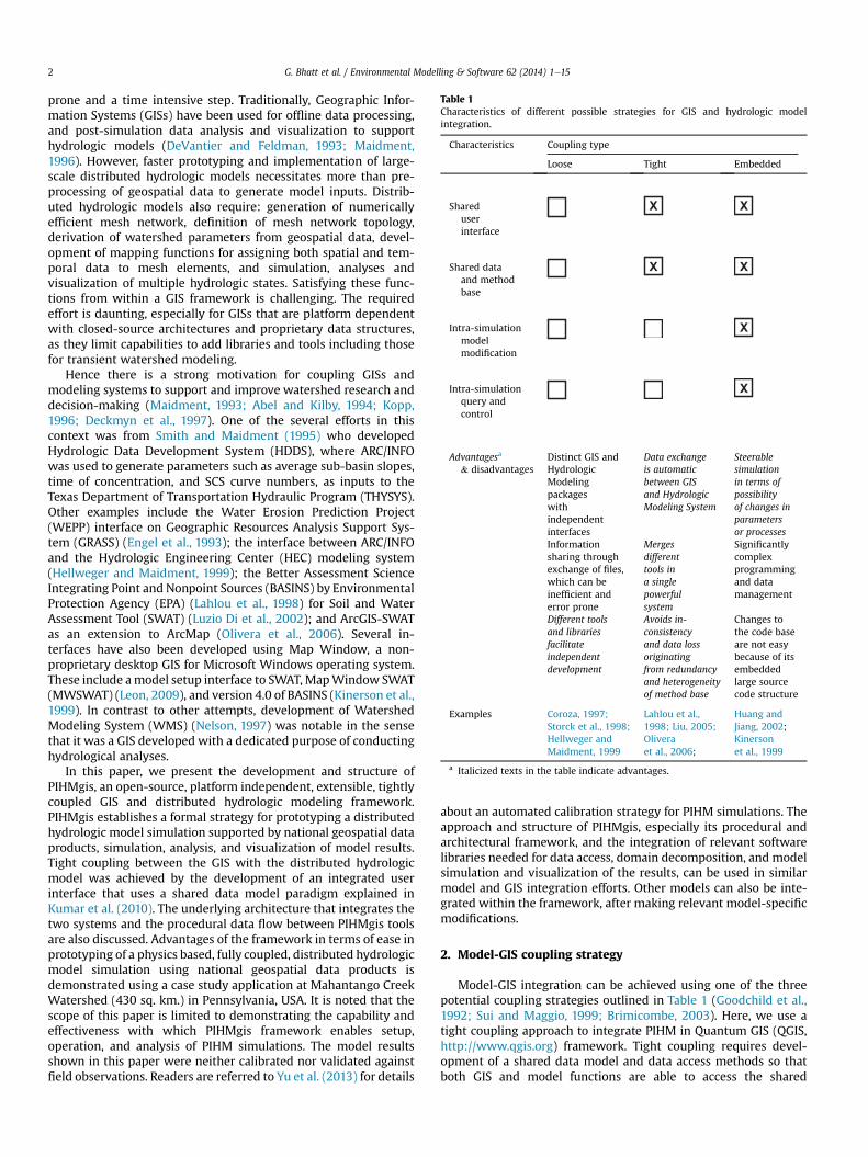
Table 1Characteristics of different possible strategies for GIS and hydrologic modelintegration.

Characteristics Coupling type

Loose Tight Embedded

Shareduserinterface

Shared dataand methodbase

Intra-simulationmodelmodification

Intra-simulationquery andcontrol

Advantagesa

& disadvantagesDistinct GIS andHydrologicModelingpackageswithindependentinterfaces

Data exchangeis automaticbetween GISand HydrologicModeling System

Steerablesimulationin terms ofpossibilityof changes inparametersor processes

Informationsharing throughexchange of files,which can beinefficient anderror prone

Mergesdifferenttools ina singlepowerfulsystem

Significantlycomplexprogrammingand datamanagement

Different toolsand librariesfacilitateindependentdevelopment

Avoids in-consistencyand data lossoriginatingfrom redundancyand heterogeneityof method base

Changes tothe code baseare not easybecause of itsembeddedlarge sourcecode structure

Examples Coroza, 1997;Storck et al., 1998;Hellweger andMaidment, 1999

Lahlou et al.,1998; Liu, 2005;Oliveraet al., 2006;

Huang andJiang, 2002;Kinersonet al., 1999

a Italicized texts in the table indicate advantages.

G. Bhatt et al. / Environmental Modelling & Software 62 (2014) 1e152

prone and a time intensive step. Traditionally, Geographic Infor-mation Systems (GISs) have been used for offline data processing,and post-simulation data analysis and visualization to supporthydrologic models (DeVantier and Feldman, 1993; Maidment,1996). However, faster prototyping and implementation of large-scale distributed hydrologic models necessitates more than pre-processing of geospatial data to generate model inputs. Distrib-uted hydrologic models also require: generation of numericallyefficient mesh network, definition of mesh network topology,derivation of watershed parameters from geospatial data, devel-opment of mapping functions for assigning both spatial and tem-poral data to mesh elements, and simulation, analyses andvisualization of multiple hydrologic states. Satisfying these func-tions from within a GIS framework is challenging. The requiredeffort is daunting, especially for GISs that are platform dependentwith closed-source architectures and proprietary data structures,as they limit capabilities to add libraries and tools including thosefor transient watershed modeling.

Hence there is a strong motivation for coupling GISs andmodeling systems to support and improve watershed research anddecision-making (Maidment, 1993; Abel and Kilby, 1994; Kopp,1996; Deckmyn et al., 1997). One of the several efforts in thiscontext was from Smith and Maidment (1995) who developedHydrologic Data Development System (HDDS), where ARC/INFOwas used to generate parameters such as average sub-basin slopes,time of concentration, and SCS curve numbers, as inputs to theTexas Department of Transportation Hydraulic Program (THYSYS).Other examples include the Water Erosion Prediction Project(WEPP) interface on Geographic Resources Analysis Support Sys-tem (GRASS) (Engel et al., 1993); the interface between ARC/INFOand the Hydrologic Engineering Center (HEC) modeling system(Hellweger and Maidment, 1999); the Better Assessment ScienceIntegrating Point and Nonpoint Sources (BASINS) by EnvironmentalProtection Agency (EPA) (Lahlou et al., 1998) for Soil and WaterAssessment Tool (SWAT) (Luzio Di et al., 2002); and ArcGIS-SWATas an extension to ArcMap (Olivera et al., 2006). Several in-terfaces have also been developed using Map Window, a non-proprietary desktop GIS for Microsoft Windows operating system.These include amodel setup interface to SWAT,MapWindow SWAT(MWSWAT) (Leon, 2009), and version 4.0 of BASINS (Kinerson et al.,1999). In contrast to other attempts, development of WatershedModeling System (WMS) (Nelson, 1997) was notable in the sensethat it was a GIS developed with a dedicated purpose of conductinghydrological analyses.

In this paper, we present the development and structure ofPIHMgis, an open-source, platform independent, extensible, tightlycoupled GIS and distributed hydrologic modeling framework.PIHMgis establishes a formal strategy for prototyping a distributedhydrologic model simulation supported by national geospatial dataproducts, simulation, analysis, and visualization of model results.Tight coupling between the GIS with the distributed hydrologicmodel was achieved by the development of an integrated userinterface that uses a shared data model paradigm explained inKumar et al. (2010). The underlying architecture that integrates thetwo systems and the procedural data flow between PIHMgis toolsare also discussed. Advantages of the framework in terms of ease inprototyping of a physics based, fully coupled, distributed hydrologicmodel simulation using national geospatial data products isdemonstrated using a case study application at Mahantango CreekWatershed (430 sq. km.) in Pennsylvania, USA. It is noted that thescope of this paper is limited to demonstrating the capability andeffectiveness with which PIHMgis framework enables setup,operation, and analysis of PIHM simulations. The model resultsshown in this paper were neither calibrated nor validated againstfield observations. Readers are referred to Yu et al. (2013) for details

about an automated calibration strategy for PIHM simulations. Theapproach and structure of PIHMgis, especially its procedural andarchitectural framework, and the integration of relevant softwarelibraries needed for data access, domain decomposition, and modelsimulation and visualization of the results, can be used in similarmodel and GIS integration efforts. Other models can also be inte-grated within the framework, after making relevant model-specificmodifications.

2. Model-GIS coupling strategy

Model-GIS integration can be achieved using one of the threepotential coupling strategies outlined in Table 1 (Goodchild et al.,1992; Sui and Maggio, 1999; Brimicombe, 2003). Here, we use atight coupling approach to integrate PIHM in Quantum GIS (QGIS,http://www.qgis.org) framework. Tight coupling requires devel-opment of a shared data model and data access methods so thatboth GIS and model functions are able to access the shared

G. Bhatt et al. / Environmental Modelling & Software 62 (2014) 1e15 3

geodatabase. Shared data model concept has been previously usedin ArcHydro (Maidment, 2002) to process and develop geospatialdata that can be henceforth used in hydraulic and hydrologic an-alyses. The tight coupling strategy has the advantage of indepen-dent development of both GIS and the hydrologic model, as is thecharacteristic of loosely coupled systems, while also allowingshared geospatial data access between the GIS and hydrologicmodel. The two systems are linked through object oriented toolsthat mimicmany of the advantages of an embedded system, such asproviding access to model parameters.

2.1. GIS framework

QGIS was used as the GIS platform to perform GIS-Model inte-gration. The selection of QGIS was based on multiple factorsincluding: its compatibility with multiple operating systems(Microsoft Windows, Macintosh, Linux etc.), an uncluttered userfriendly interface, easy plugin-development functionality, supportof wide range of data formats, an active developer community tosupport state-of-the-art software and hardware developments, andfinally its open-source structure that allow function calls to models,data and numerical libraries. QGIS has been developed in Cþþ andextensively uses Qt (http://trolltech.com/products/qt) and Pythonlibraries. It is comprised of four major subsystems: (1) input/cap-ture; (2) management; (3) manipulation/analysis; and (4) output/display. The data input/capture subsystem, provides operationalfunctions for reading, collecting, capturing, and querying geospatialdata. The data management subsystem organizes and stores spatialdata and their attributes to enable efficient query and quickretrieval for display, processing, and analysis. It also manages themodification and update of existing databases through editingtools. The manipulation and analysis subsystem executes thetransformation of data from one form to another depending onmodel applications. The data display subsystem provides visualaids for quick interpretation of geospatial data in the form of dia-grams, maps, or tables as well as data output providing access to theanalyzed data in one of the several supported file formats.

The data management subsystem of QGIS offers an easy linkpoint for integration with the hydrologic model through develop-ment of shared data structures that define both GIS feature objectsand hydrologic features in the model. The data model for a GISincludes constructs for spatial data, topological data, and attributedata (Nyerges, 1987). In contrast, data structure of hydrologic fea-tures is determined by the topological relations between physio-graphic prototypes and coupling between processes. Open-sourceaccess to a QGIS facilitates the development and use of native QGISclasses and functions, which offer the interface and linkagesnecessary for supporting data structures of both GIS and hydrologicfeature objects.

2.2. Hydrologic modeling framework

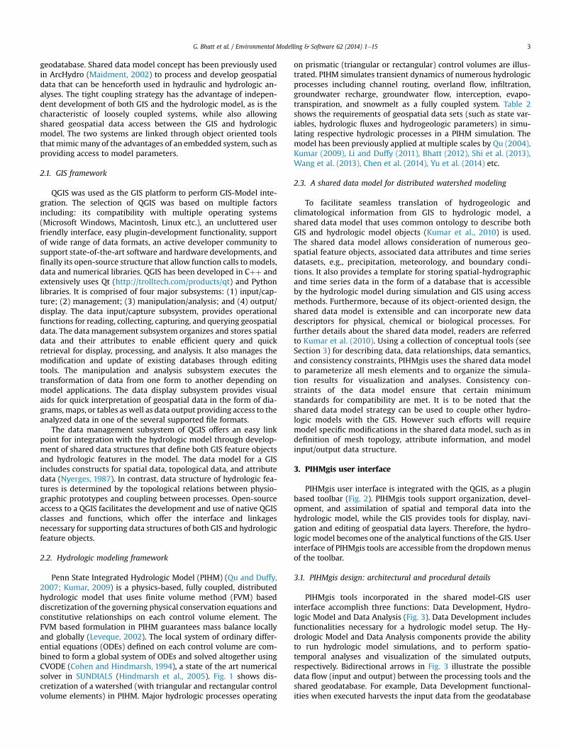
Penn State Integrated Hydrologic Model (PIHM) (Qu and Duffy,2007; Kumar, 2009) is a physics-based, fully coupled, distributedhydrologic model that uses finite volume method (FVM) baseddiscretization of the governing physical conservation equations andconstitutive relationships on each control volume element. TheFVM based formulation in PIHM guarantees mass balance locallyand globally (Leveque, 2002). The local system of ordinary differ-ential equations (ODEs) defined on each control volume are com-bined to form a global system of ODEs and solved altogether usingCVODE (Cohen and Hindmarsh, 1994), a state of the art numericalsolver in SUNDIALS (Hindmarsh et al., 2005). Fig. 1 shows dis-cretization of a watershed (with triangular and rectangular controlvolume elements) in PIHM. Major hydrologic processes operating

on prismatic (triangular or rectangular) control volumes are illus-trated. PIHM simulates transient dynamics of numerous hydrologicprocesses including channel routing, overland flow, infiltration,groundwater recharge, groundwater flow, interception, evapo-transpiration, and snowmelt as a fully coupled system. Table 2shows the requirements of geospatial data sets (such as state var-iables, hydrologic fluxes and hydrogeologic parameters) in simu-lating respective hydrologic processes in a PIHM simulation. Themodel has been previously applied at multiple scales by Qu (2004),Kumar (2009), Li and Duffy (2011), Bhatt (2012), Shi et al. (2013),Wang et al. (2013), Chen et al. (2014), Yu et al. (2014) etc.

2.3. A shared data model for distributed watershed modeling

To facilitate seamless translation of hydrogeologic andclimatological information from GIS to hydrologic model, ashared data model that uses common ontology to describe bothGIS and hydrologic model objects (Kumar et al., 2010) is used.The shared data model allows consideration of numerous geo-spatial feature objects, associated data attributes and time seriesdatasets, e.g., precipitation, meteorology, and boundary condi-tions. It also provides a template for storing spatial-hydrographicand time series data in the form of a database that is accessibleby the hydrologic model during simulation and GIS using accessmethods. Furthermore, because of its object-oriented design, theshared data model is extensible and can incorporate new datadescriptors for physical, chemical or biological processes. Forfurther details about the shared data model, readers are referredto Kumar et al. (2010). Using a collection of conceptual tools (seeSection 3) for describing data, data relationships, data semantics,and consistency constraints, PIHMgis uses the shared data modelto parameterize all mesh elements and to organize the simula-tion results for visualization and analyses. Consistency con-straints of the data model ensure that certain minimumstandards for compatibility are met. It is to be noted that theshared data model strategy can be used to couple other hydro-logic models with the GIS. However such efforts will requiremodel specific modifications in the shared data model, such as indefinition of mesh topology, attribute information, and modelinput/output data structure.

3. PIHMgis user interface

PIHMgis user interface is integrated with the QGIS, as a pluginbased toolbar (Fig. 2). PIHMgis tools support organization, devel-opment, and assimilation of spatial and temporal data into thehydrologic model, while the GIS provides tools for display, navi-gation and editing of geospatial data layers. Therefore, the hydro-logic model becomes one of the analytical functions of the GIS. Userinterface of PIHMgis tools are accessible from the dropdownmenusof the toolbar.

3.1. PIHMgis design: architectural and procedural details

PIHMgis tools incorporated in the shared model-GIS userinterface accomplish three functions: Data Development, Hydro-logic Model and Data Analysis (Fig. 3). Data Development includesfunctionalities necessary for a hydrologic model setup. The Hy-drologic Model and Data Analysis components provide the abilityto run hydrologic model simulations, and to perform spatio-temporal analyses and visualization of the simulated outputs,respectively. Bidirectional arrows in Fig. 3 illustrate the possibledata flow (input and output) between the processing tools and theshared geodatabase. For example, Data Development functional-ities when executed harvests the input data from the geodatabase

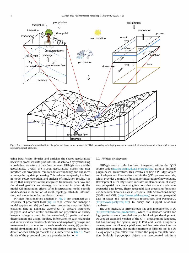
Fig. 1. Discretization of a watershed into triangular and linear mesh elements in PIHM. Interacting hydrologic processes are coupled within each control volume and betweenneighboring mesh elements.

G. Bhatt et al. / Environmental Modelling & Software 62 (2014) 1e154

using Data Access libraries and enriches the shared geodatabasebackwith processed data products. This is achieved by synthesizinga predefined structure of data flow between PIHMgis tools and thegeodatabase. Overall the shared geodatabase makes the userinterface less error prone, removes data redundancy, and enhancesaccuracy during data processing. This reduces complexity involvedin model setup, operation, and analysis of simulation results. It isnoted that subsystems of the integrated framework, data flow andthe shared geodatabase strategy can be used in other similarmodel-GIS integration efforts, after incorporating model-specificmodifications in definition of mesh topology, attribute informa-tion, and model input/output data structure.

PIHMgis functionalities detailed in Fig. 3 are organized as asequence of procedural tools (Fig. 4) to (a) create and manage amodel application; (b) perform raster processing steps on digitalelevation data to delineate watershed; (c) prepare watershedpolygons and other vector constraints for generation of qualityirregular triangular mesh for the watershed; (d) perform domaindiscretization and assign topology information to each triangularand linear mesh elements; (e) estimate andmap hydrogeologic andmeteorological parameters to each mesh elements; (f) performmodel simulation; and (g) analyze simulation outputs. Functionaldetails of each PIHMgis toolsets are summarized in Table 3. Moredetails of the procedural tools are provided in Section 4.

3.2. PIHMgis development

PIHMgis source code has been integrated within the QGISsource code (http://download.qgis.org/qgis/src/) using an internalplugin-based architecture. This involves calling a PIHMgis objectand its dependent libraries fromwithin the QGIS open-source code,which provides a template function for integration of new plugins.Development of PIHMgis tools includes implementation of manynew geospatial data processing functions that can read and creategeospatial data layers. These geospatial data processing functionsuse dependent libraries such as Geospatial Data Abstraction Library(GDAL) and OGR (http://www.gdal.org/ogr/) to access geospatialdata in raster and vector formats respectively, and PostgreSQL(http://www.postgresql.org) to query and support relationaldatabases.

The user interface of PIHMgis tools has been implemented in Qt(http://trolltech.com/products/qt), which is a standard toolkit forhigh performance, cross-platform graphical widget development.Qt uses an extended version of the Cþþ programming language,but has bindings for Python, Ruby, C, Perl, and Pascal. It supportsdevelopment on all major platforms, and has extensive interna-tionalization support. The graphic interface of PIHMgis tool is a Qtdialog object, again called from within the plugin template func-tion. Multiple input/output objects are incorporated within a

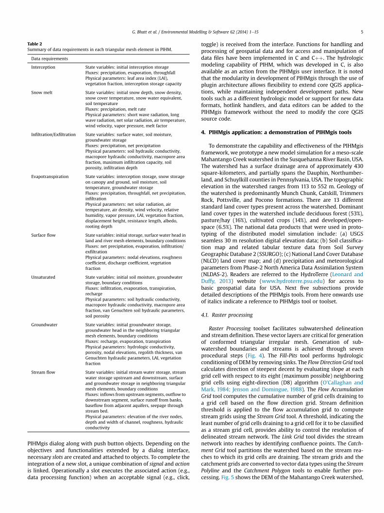
Table 2Summary of data requirements in each triangular mesh element in PIHM.

Data requirements

Interception State variables: initial interception storageFluxes: precipitation, evaporation, throughfallPhysical parameters: leaf area index (LAI),vegetation fraction, interception storage capacity

Snow melt State variables: initial snow depth, snow density,snow cover temperature, snow water equivalent,soil temperatureFluxes: precipitation, melt ratePhysical parameters: short wave radiation, longwave radiation, net solar radiation, air temperature,wind velocity, vapor pressure, melt factor

Infiltration/Exfiltration State variables: surface water, soil moisture,groundwater storageFluxes: precipitation, net precipitationPhysical parameters: soil hydraulic conductivity,macropore hydraulic conductivity, macropore areafraction, maximum infiltration capacity, soilporosity, infiltration depth

Evapotranspiration State variables: interception storage, snow storageon canopy and ground, soil moisture, soiltemperature, groundwater storageFluxes: precipitation, throughfall, net precipitation,infiltrationPhysical parameters: net solar radiation, airtemperature, air density, wind velocity, relativehumidity, vapor pressure, LAI, vegetation fraction,displacement height, resistance length, albedo,rooting depth

Surface flow State variables: initial storage, surface water head inland and river mesh elements, boundary conditionsFluxes: net precipitation, evaporation, infiltration/exfiltrationPhysical parameters: nodal elevations, roughnesscoefficient, discharge coefficient, vegetationfraction

Unsaturated State variables: initial soil moisture, groundwaterstorage, boundary conditionsFluxes: infiltration, evaporation, transpiration,rechargePhysical parameters: soil hydraulic conductivity,macropore hydraulic conductivity, macropore areafraction, van Genuchten soil hydraulic parameters,soil porosity

Groundwater State variables: initial groundwater storage,groundwater head in the neighboring triangularmesh elements, boundary conditionsFluxes: recharge, evaporation, transpirationPhysical parameters: hydrologic conductivity,porosity, nodal elevations, regolith thickness, vanGenuchten hydraulic parameters, LAI, vegetationfraction

Stream flow State variables: initial stream water storage, streamwater storage upstream and downstream, surfaceand groundwater storage in neighboring triangularmesh elements, boundary conditionsFluxes: inflows from upstream segments, outflow todownstream segment, surface runoff from banks,baseflow from adjacent aquifers, seepage throughstream bed.Physical parameters: elevation of the river nodes,depth and width of channel, roughness, hydraulicconductivity

G. Bhatt et al. / Environmental Modelling & Software 62 (2014) 1e15 5

PIHMgis dialog along with push button objects. Depending on theobjectives and functionalities extended by a dialog interface,necessary slots are created and attached to objects. To complete theintegration of a new slot, a unique combination of signal and actionis linked. Operationally a slot executes the associated action (e.g.,data processing function) when an acceptable signal (e.g., click,

toggle) is received from the interface. Functions for handling andprocessing of geospatial data and for access and manipulation ofdata files have been implemented in C and Cþþ. The hydrologicmodeling capability of PIHM, which was developed in C, is alsoavailable as an action from the PIHMgis user interface. It is notedthat the modularity in development of PIHMgis through the use ofplugin architecture allows flexibility to extend core QGIS applica-tions, while maintaining independent development paths. Newtools such as a different hydrologic model or support for new dataformats, hotlink handlers, and data editors can be added to thePIHMgis framework without the need to modify the core QGISsource code.

4. PIHMgis application: a demonstration of PIHMgis tools

To demonstrate the capability and effectiveness of the PIHMgisframework, we prototype a newmodel simulation for a meso-scaleMahantango Creekwatershed in the Susquehanna River Basin, USA.The watershed has a surface drainage area of approximately 430square-kilometers, and partially spans the Dauphin, Northumber-land, and Schuylkill counties in Pennsylvania, USA. The topographicelevation in the watershed ranges from 113 to 552 m. Geology ofthe watershed is predominantly Munch Chunk, Catskill, TrimmersRock, Pottsville, and Pocono formations. There are 13 differentstandard land cover types present across the watershed. Dominantland cover types in the watershed include deciduous forest (53%),pasture/hay (16%), cultivated crops (14%), and developed/open-space (6.5%). The national data products that were used in proto-typing of the distributed model simulation include: (a) USGSseamless 30 m resolution digital elevation data; (b) Soil classifica-tion map and related tabular texture data from Soil SurveyGeographic Database 2 (SSURGO); (c) National Land Cover Database(NLCD) land cover map; and (d) precipitation and meteorologicalparameters from Phase-2 North America Data Assimilation System(NLDAS-2). Readers are referred to the HydroTerre (Leonard andDuffy, 2013) website (www.hydroterre.psu.edu) for access tobasic geospatial data for USA. Next five subsections providedetailed descriptions of the PIHMgis tools. From here onwards useof italics indicate a reference to PIHMgis tool or toolset.

4.1. Raster processing

Raster Processing toolset facilitates subwatershed delineationand stream definition. These vector layers are critical for generationof conformed triangular irregular mesh. Generation of sub-watershed boundaries and streams is achieved through sevenprocedural steps (Fig. 4). The Fill-Pits tool performs hydrologicconditioning of DEMby removing sinks. The FlowDirection Grid toolcalculates direction of steepest decent by evaluating slope at eachgrid cell with respect to its eight (maximum possible) neighboringgrid cells using eight-direction (D8) algorithm (O'Callaghan andMark, 1984; Jenson and Domingue, 1988). The Flow AccumulationGrid tool computes the cumulative number of grid cells draining toa grid cell based on the flow direction grid. Stream definitionthreshold is applied to the flow accumulation grid to computestream grids using the Stream Grid tool. A threshold, indicating theleast number of grid cells draining to a grid cell for it to be classifiedas a stream grid cell, provides ability to control the resolution ofdelineated stream network. The Link Grid tool divides the streamnetwork into reaches by identifying confluence points. The Catch-ment Grid tool partitions the watershed based on the stream rea-ches to which its grid cells are draining. The stream grids and thecatchment grids are converted to vector data types using the StreamPolyline and the Catchment Polygon tools to enable further pro-cessing. Fig. 5 shows the DEM of the Mahantango Creek watershed,

Fig. 2. The PIHMgis user interface within QGIS. (a) PIHMgis toolbar includes data processing and modeling system components. (b) The data frame displays raster/vector geospatialdatasets. Shown in the data frame are stream network, watershed boundary, and triangular irregular mesh for Mahantango Creek watershed.

G. Bhatt et al. / Environmental Modelling & Software 62 (2014) 1e156

which is the only input required in Raster Processing apart from thestreams definition threshold. Fig. 5 shows the catchment boundaryand stream network obtained from digital elevation dataset usingRaster Processing toolset. Here, the stream grids were generatedusing 4000 grid cells (equivalent to a drainage area of 3.6 sq. km.) asthe threshold. RunAll combines all of the procedural data process-ing steps of Raster Processing into a single tool.

4.2. Vector processing

Vector Processing provides tools to condition and consolidatemultiple hydrologic features into one vector layer, so that they canbe used for generating quality triangular mesh. Consolidation in-cludes merging of watershed boundary, stream network, and otherrelevant vector objects such as nodes (stream gauge, groundwaterobservation well locations), polygons (soil classification, land use,political boundaries) and polylines (artificial channels or drainagenetworks). Data processing steps involved in the Vector Processingare illustrated in Fig. 4. The Dissolve Polygon is an optional dataprocessing tool that may be used to remove the internal (e.g.,subwatershed) boundaries, if needed. The Polygon to Polyline toolconverts the input polygon watershed features, which are polygonvector objects, to their polyline equivalents. This step is neededbecause a simplification operation only works on watershed

features that are polylines. The Polygon to Polyline tool preservesthe external boundaries of polygons as polyline equivalents. TheSimplify Line tool removes unwanted irregularities from a polylineby removing unnecessary nodes (Douglas and Peucker, 1973) basedon specified simplification tolerance length as shown in Fig. 6a. Thereduction in number of nodes for representation of polylines de-creases the number of generated mesh elements around it. It is tobe noted that simplification tolerance is selected such thatsemblance of the constraining polyline is maintained. For illustra-tion purposes a qualitative comparison between unsimplified andsimplified watershed features has been shown in Fig. 6b. Theillustration shows that the aliasing effects that are introduced inwatershed boundary and stream features during the Raster Pro-cessing are overcome by simplification. This results in significantdecrease in the number of triangular elements in generated meshas compared to one generated using unsimplified watershed fea-tures (Fig. 6b). Next, polylines are split into lines by separating themat the vertices through the Split Line tool. The Vector Merge toolcombines all feature objects into a single vector layer. Fig. 7 showssimplified and consolidated output from Vector Processing for theMahantango Creek watershed. Here, only the external catchmentboundary and stream network were considered as constraints.Streams and watershed boundary were preferentially simplifiedusing a tolerance length of 50 m and 100 m respectively.

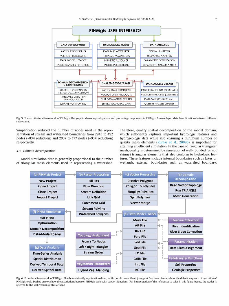
Fig. 3. The architectural framework of PIHMgis. The graphic shows key subsystems and processing components in PIHMgis. Arrows depict data flow directions between differentsubsystems.

G. Bhatt et al. / Environmental Modelling & Software 62 (2014) 1e15 7

Simplification reduced the number of nodes used in the repre-sentation of stream and watershed boundaries from 2945 to 492nodes (~83% reduction) and 2937 to 177 nodes (~93% reduction)respectively.

4.3. Domain decomposition

Model simulation time is generally proportional to the numberof triangular mesh elements used in representing a watershed.

Fig. 4. Procedural framework of PIHMgis. Blue boxes identify key functionalities, while purpPIHMgis tools. Dashed arrows show the associations between PIHMgis tools with support fureferred to the web version of this article.)

Therefore, quality spatial decomposition of the model domain,which sufficiently captures important hydrologic features andhydrogeologic data while also ensuring a minimum number ofquality mesh elements (Kumar et al., 2009b), is important forattaining an efficient simulation. In the case of irregular triangularmesh, quality is determined by generation of well-rounded (or notskinny) triangular elements that also conform to hydrologic fea-tures. These features include internal boundaries such as lakes orwetlands, external boundaries such as watershed boundary,

le boxes identify support functions. Arrows show the default sequence of execution ofnctions. (For interpretation of the references to color in this figure legend, the reader is

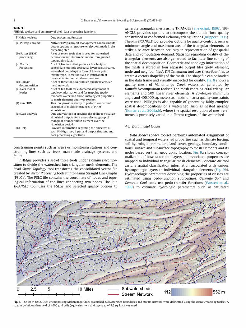
Table 3PIHMgis toolsets and summary of their data processing functions.

PIHMgis toolsets Data processing function

(a) PIHMgis project Native PIHMgis project management handles input/output options in response to selectionsmade in thepreceding step.

(b) Raster (DEM)processing

A set of seven tools that is used for watersheddelineation and stream definition from griddedtopographic data.

(c) VectorProcessing

A set of five tools that provides flexibility toconsolidate multiple geospatial layers (e.g., streams,watershed boundary) in form of line or pointfeature type. These tools aid in generation ofconstraints for domain decomposition.

(d) Domaindecomposition

A set of three tools to produce quality triangularmesh network.

(e) Data modelloader

A set of ten tools for automated assignment oftopology information and for mapping spatio-temporal watershed and climatological propertiesto mesh elements and river reaches.

(f) Run PIHM This tool provides ability to perform concurrentexecution of multiple instances of PIHMsimulations.

(g) Data analysis Data analysis toolset provides the ability to visualizesimulated outputs for a user-selected group oftriangular or linear mesh element over thesimulation period.

(h) Help Provides information regarding the objective ofeach PIHMgis tool, input and output datasets, anddata processing algorithms.

G. Bhatt et al. / Environmental Modelling & Software 62 (2014) 1e158

constraining points such as weirs or monitoring stations and con-straining lines such as rivers, man made drainage systems, andfaults.

PIHMgis provides a set of three tools under Domain Decompo-sition to divide the watershed into triangular mesh elements. TheRead Shape Topology tool transforms the consolidated vector filecreated by Vector Processing toolset into Planar Straight Line Graphs(PSLGs). The PSLG file contains the coordinate of nodes and topo-logical information of the lines connecting two nodes. The RunTRIANGLE tool uses the PSLGs and selected quality options to

Fig. 5. The 30-m USGS DEM encompassing Mahantango Creek watershed. Subwatershed bstream definition threshold of 4000 grid cells (equivalent to a drainage area of 3.6 sq. km.)

generate triangular mesh using TRIANGLE (Shewchuk, 1996). TRI-ANGLE provides options to decompose the domain into qualityconstrained or conformed Delaunay triangulations (Ruppert, 1995).The RunTRIANGLE tool provides options for quality controls, such asminimum angle and maximum area of the triangular elements, tostrike a balance between accuracy in representation of geospatialdata and computation demand. Statistics regarding quality of thetriangular elements are also generated to facilitate fine-tuning ofthe spatial decomposition. Geometric and topology information ofthe mesh is stored in four separate output files (poly, element,node, and neighbor files). TIN Generation tool uses these four files tocreate a vector (shapefile) of the mesh. The shapefile can be loadedin the data frame and visually inspected for quality. Fig. 8 shows aquality mesh of Mahantango Creek watershed generated byDomain Decomposition toolset. The mesh contains 2606 triangularelements and 509 linear river elements. A 20-degree minimumangle and 400,000 sq. meters as maximum area quality constraintswere used. PIHMgis is also capable of generating fairly complexspatial decompositions of a watershed such as nested meshes(Kumar et al., 2009a,b), where the spatial resolution of mesh ele-ments is purposely varied in different regions of the watershed.

4.4. Data model loader

Data Model Loader toolset performs automated assignment ofspatial and temporal watershed properties such as climate forcing,soil hydrologic parameters, land cover, geology, boundary condi-tions, surface and subsurface topography to mesh elements and itsnodes based on their geographic location. Fig. 9a shows concep-tualization of how raster data layers and associated properties aremapped to individual triangular mesh elements. Generate Att toolassigns spatial classification information associated with varioushydrogeologic layers to individual triangular elements (Fig. 9b).Hydrogeologic parameters describing the properties of classes areestimated using pedo-function subroutines. Generate Soil andGenerate Geol tools use pedo-transfer functions (Wosten et al.,1999) to estimate hydrologic parameters such as saturated

oundaries and stream network were delineated using the Raster Processing toolset. Awas used.

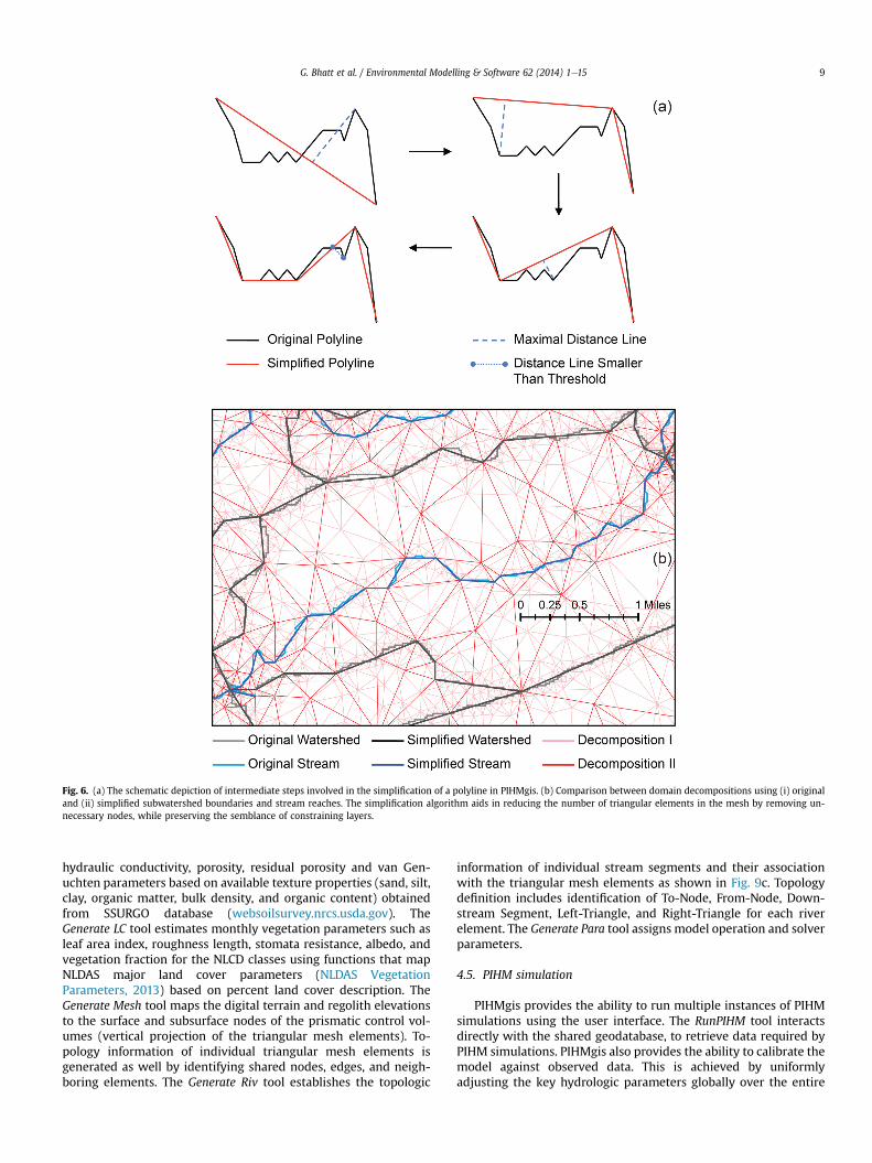
Fig. 6. (a) The schematic depiction of intermediate steps involved in the simplification of a polyline in PIHMgis. (b) Comparison between domain decompositions using (i) originaland (ii) simplified subwatershed boundaries and stream reaches. The simplification algorithm aids in reducing the number of triangular elements in the mesh by removing un-necessary nodes, while preserving the semblance of constraining layers.

G. Bhatt et al. / Environmental Modelling & Software 62 (2014) 1e15 9

hydraulic conductivity, porosity, residual porosity and van Gen-uchten parameters based on available texture properties (sand, silt,clay, organic matter, bulk density, and organic content) obtainedfrom SSURGO database (websoilsurvey.nrcs.usda.gov). TheGenerate LC tool estimates monthly vegetation parameters such asleaf area index, roughness length, stomata resistance, albedo, andvegetation fraction for the NLCD classes using functions that mapNLDAS major land cover parameters (NLDAS VegetationParameters, 2013) based on percent land cover description. TheGenerate Mesh tool maps the digital terrain and regolith elevationsto the surface and subsurface nodes of the prismatic control vol-umes (vertical projection of the triangular mesh elements). To-pology information of individual triangular mesh elements isgenerated as well by identifying shared nodes, edges, and neigh-boring elements. The Generate Riv tool establishes the topologic

information of individual stream segments and their associationwith the triangular mesh elements as shown in Fig. 9c. Topologydefinition includes identification of To-Node, From-Node, Down-stream Segment, Left-Triangle, and Right-Triangle for each riverelement. The Generate Para tool assigns model operation and solverparameters.

4.5. PIHM simulation

PIHMgis provides the ability to run multiple instances of PIHMsimulations using the user interface. The RunPIHM tool interactsdirectly with the shared geodatabase, to retrieve data required byPIHM simulations. PIHMgis also provides the ability to calibrate themodel against observed data. This is achieved by uniformlyadjusting the key hydrologic parameters globally over the entire

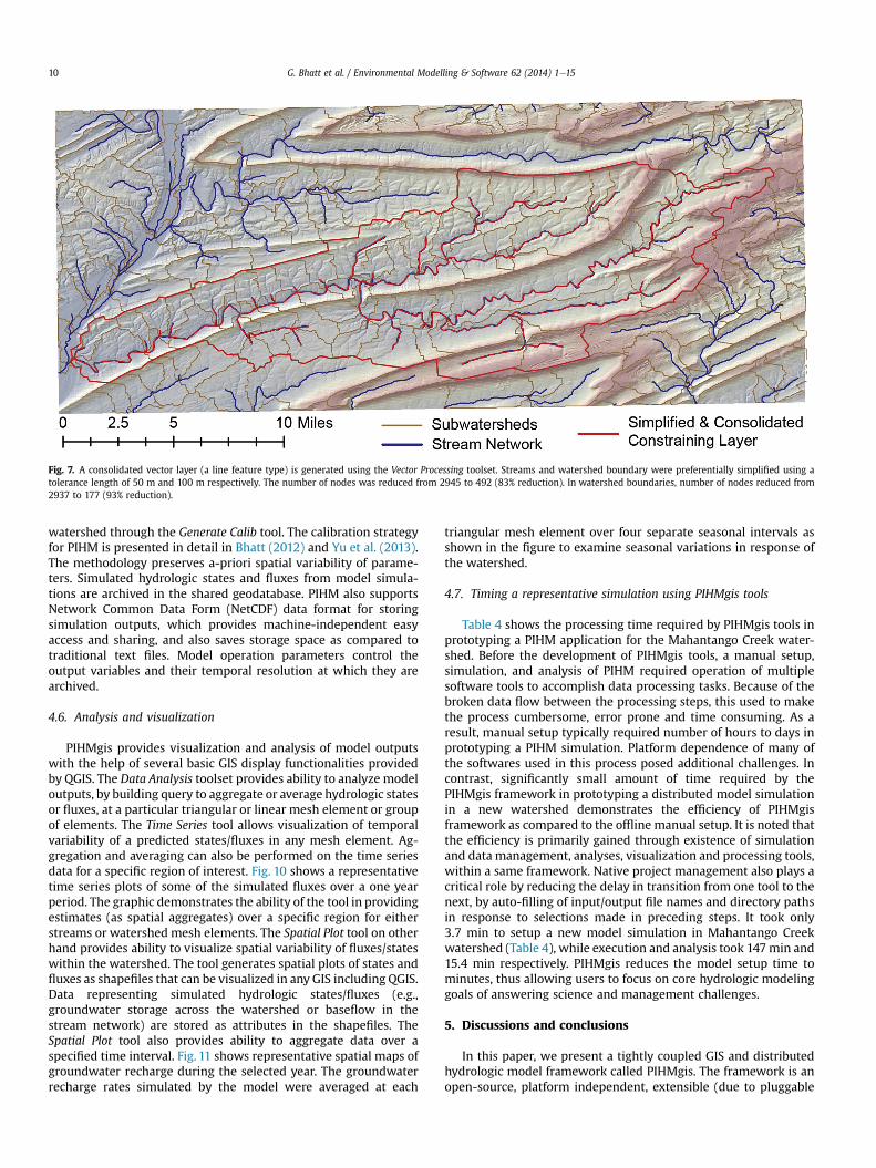
Fig. 7. A consolidated vector layer (a line feature type) is generated using the Vector Processing toolset. Streams and watershed boundary were preferentially simplified using atolerance length of 50 m and 100 m respectively. The number of nodes was reduced from 2945 to 492 (83% reduction). In watershed boundaries, number of nodes reduced from2937 to 177 (93% reduction).

G. Bhatt et al. / Environmental Modelling & Software 62 (2014) 1e1510

watershed through the Generate Calib tool. The calibration strategyfor PIHM is presented in detail in Bhatt (2012) and Yu et al. (2013).The methodology preserves a-priori spatial variability of parame-ters. Simulated hydrologic states and fluxes from model simula-tions are archived in the shared geodatabase. PIHM also supportsNetwork Common Data Form (NetCDF) data format for storingsimulation outputs, which provides machine-independent easyaccess and sharing, and also saves storage space as compared totraditional text files. Model operation parameters control theoutput variables and their temporal resolution at which they arearchived.

4.6. Analysis and visualization

PIHMgis provides visualization and analysis of model outputswith the help of several basic GIS display functionalities providedby QGIS. The Data Analysis toolset provides ability to analyze modeloutputs, by building query to aggregate or average hydrologic statesor fluxes, at a particular triangular or linear mesh element or groupof elements. The Time Series tool allows visualization of temporalvariability of a predicted states/fluxes in any mesh element. Ag-gregation and averaging can also be performed on the time seriesdata for a specific region of interest. Fig. 10 shows a representativetime series plots of some of the simulated fluxes over a one yearperiod. The graphic demonstrates the ability of the tool in providingestimates (as spatial aggregates) over a specific region for eitherstreams or watershed mesh elements. The Spatial Plot tool on otherhand provides ability to visualize spatial variability of fluxes/stateswithin the watershed. The tool generates spatial plots of states andfluxes as shapefiles that can be visualized in any GIS including QGIS.Data representing simulated hydrologic states/fluxes (e.g.,groundwater storage across the watershed or baseflow in thestream network) are stored as attributes in the shapefiles. TheSpatial Plot tool also provides ability to aggregate data over aspecified time interval. Fig. 11 shows representative spatial maps ofgroundwater recharge during the selected year. The groundwaterrecharge rates simulated by the model were averaged at each

triangular mesh element over four separate seasonal intervals asshown in the figure to examine seasonal variations in response ofthe watershed.

4.7. Timing a representative simulation using PIHMgis tools

Table 4 shows the processing time required by PIHMgis tools inprototyping a PIHM application for the Mahantango Creek water-shed. Before the development of PIHMgis tools, a manual setup,simulation, and analysis of PIHM required operation of multiplesoftware tools to accomplish data processing tasks. Because of thebroken data flow between the processing steps, this used to makethe process cumbersome, error prone and time consuming. As aresult, manual setup typically required number of hours to days inprototyping a PIHM simulation. Platform dependence of many ofthe softwares used in this process posed additional challenges. Incontrast, significantly small amount of time required by thePIHMgis framework in prototyping a distributed model simulationin a new watershed demonstrates the efficiency of PIHMgisframework as compared to the offline manual setup. It is noted thatthe efficiency is primarily gained through existence of simulationand data management, analyses, visualization and processing tools,within a same framework. Native project management also plays acritical role by reducing the delay in transition from one tool to thenext, by auto-filling of input/output file names and directory pathsin response to selections made in preceding steps. It took only3.7 min to setup a new model simulation in Mahantango Creekwatershed (Table 4), while execution and analysis took 147min and15.4 min respectively. PIHMgis reduces the model setup time tominutes, thus allowing users to focus on core hydrologic modelinggoals of answering science and management challenges.

5. Discussions and conclusions

In this paper, we present a tightly coupled GIS and distributedhydrologic model framework called PIHMgis. The framework is anopen-source, platform independent, extensible (due to pluggable

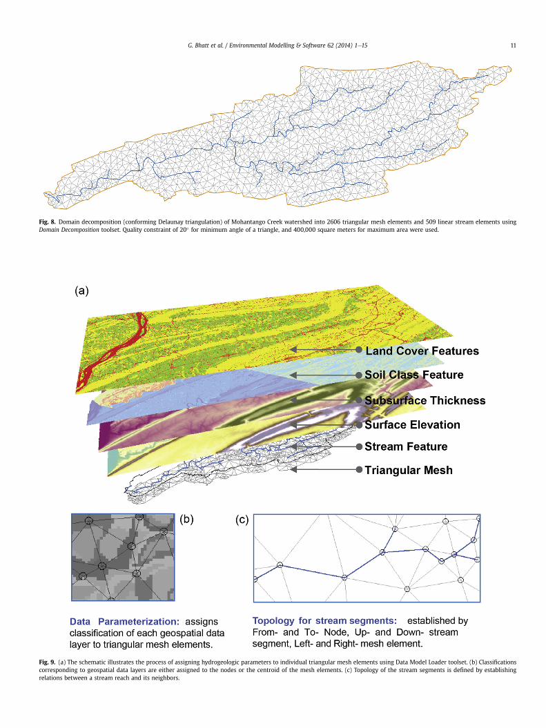
Fig. 8. Domain decomposition (conforming Delaunay triangulation) of Mohantango Creek watershed into 2606 triangular mesh elements and 509 linear stream elements usingDomain Decomposition toolset. Quality constraint of 20� for minimum angle of a triangle, and 400,000 square meters for maximum area were used.

Fig. 9. (a) The schematic illustrates the process of assigning hydrogeologic parameters to individual triangular mesh elements using Data Model Loader toolset. (b) Classificationscorresponding to geospatial data layers are either assigned to the nodes or the centroid of the mesh elements. (c) Topology of the stream segments is defined by establishingrelations between a stream reach and its neighbors.

G. Bhatt et al. / Environmental Modelling & Software 62 (2014) 1e15 11

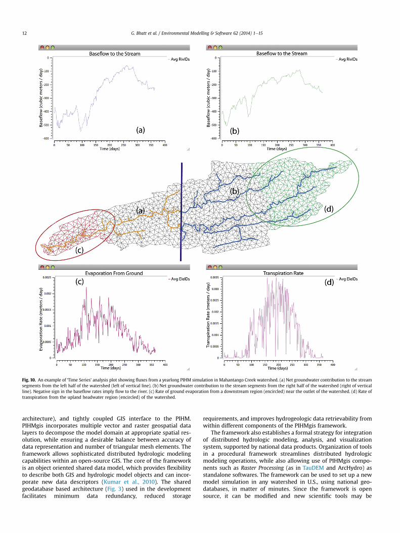
Fig. 10. An example of ‘Time Series’ analysis plot showing fluxes from a yearlong PIHM simulation in Mahantango Creek watershed. (a) Net groundwater contribution to the streamsegments from the left half of the watershed (left of vertical line). (b) Net groundwater contribution to the stream segments from the right half of the watershed (right of verticalline). Negative sign in the baseflow rates imply flow to the river. (c) Rate of ground evaporation from a downstream region (encircled) near the outlet of the watershed. (d) Rate oftranspiration from the upland headwater region (encircled) of the watershed.

G. Bhatt et al. / Environmental Modelling & Software 62 (2014) 1e1512

architecture), and tightly coupled GIS interface to the PIHM.PIHMgis incorporates multiple vector and raster geospatial datalayers to decompose the model domain at appropriate spatial res-olution, while ensuring a desirable balance between accuracy ofdata representation and number of triangular mesh elements. Theframework allows sophisticated distributed hydrologic modelingcapabilities within an open-source GIS. The core of the frameworkis an object oriented shared data model, which provides flexibilityto describe both GIS and hydrologic model objects and can incor-porate new data descriptors (Kumar et al., 2010). The sharedgeodatabase based architecture (Fig. 3) used in the developmentfacilitates minimum data redundancy, reduced storage

requirements, and improves hydrogeologic data retrievability fromwithin different components of the PIHMgis framework.

The framework also establishes a formal strategy for integrationof distributed hydrologic modeling, analysis, and visualizationsystem, supported by national data products. Organization of toolsin a procedural framework streamlines distributed hydrologicmodeling operations, while also allowing use of PIHMgis compo-nents such as Raster Processing (as in TauDEM and ArcHydro) asstandalone softwares. The framework can be used to set up a newmodel simulation in any watershed in U.S., using national geo-databases, in matter of minutes. Since the framework is opensource, it can be modified and new scientific tools may be

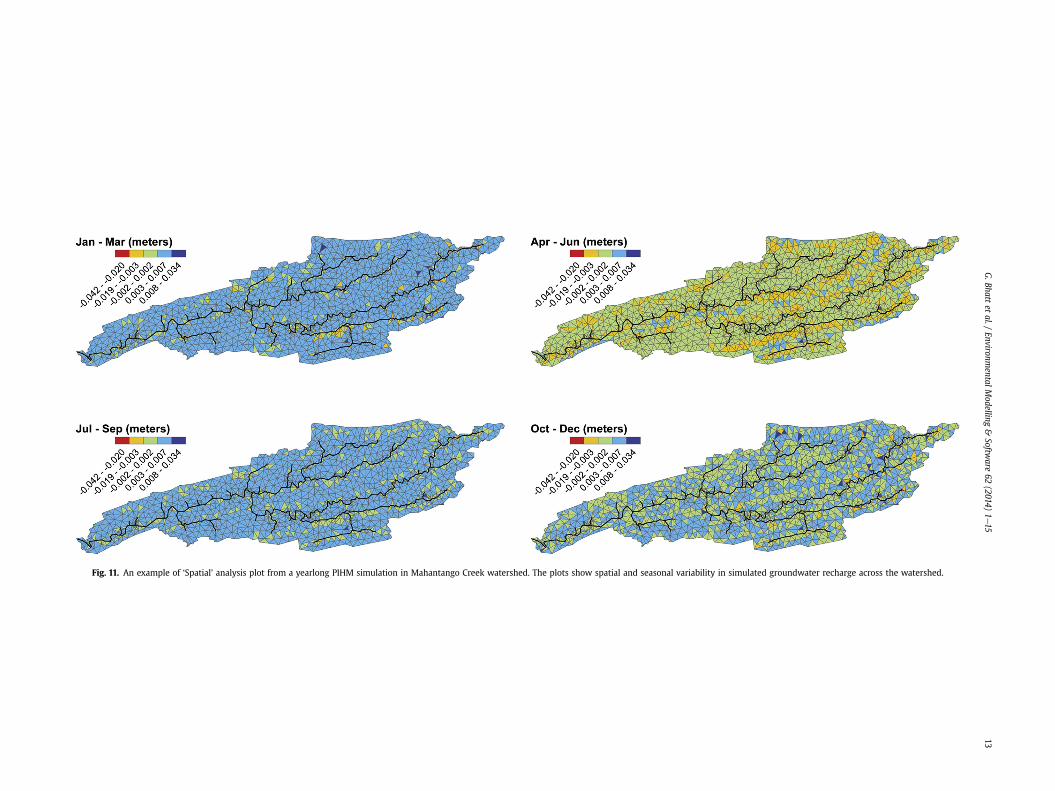
Fig. 11. An example of ‘Spatial’ analysis plot from a yearlong PIHM simulation in Mahantango Creek watershed. The plots show spatial and seasonal variability in simulated groundwater recharge across the watershed.

G.Bhatt

etal./

EnvironmentalM

odelling&

Software

62(2014)

1e15

13

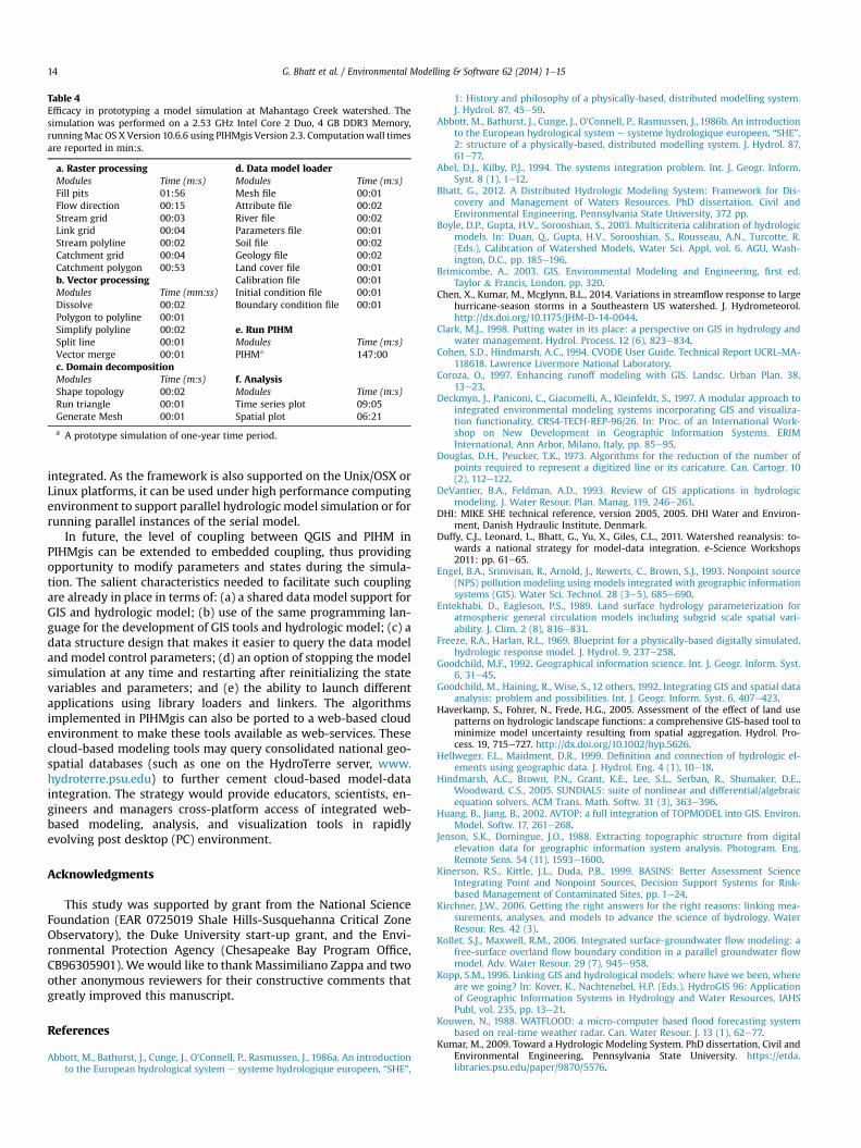
Table 4Efficacy in prototyping a model simulation at Mahantago Creek watershed. Thesimulation was performed on a 2.53 GHz Intel Core 2 Duo, 4 GB DDR3 Memory,runningMac OS X Version 10.6.6 using PIHMgis Version 2.3. Computationwall timesare reported in min:s.

a. Raster processing d. Data model loaderModules Time (m:s) Modules Time (m:s)Fill pits 01:56 Mesh file 00:01Flow direction 00:15 Attribute file 00:02Stream grid 00:03 River file 00:02Link grid 00:04 Parameters file 00:01Stream polyline 00:02 Soil file 00:02Catchment grid 00:04 Geology file 00:02Catchment polygon 00:53 Land cover file 00:01b. Vector processing Calibration file 00:01Modules Time (mm:ss) Initial condition file 00:01Dissolve 00:02 Boundary condition file 00:01Polygon to polyline 00:01Simplify polyline 00:02 e. Run PIHMSplit line 00:01 Modules Time (m:s)Vector merge 00:01 PIHMa 147:00c. Domain decompositionModules Time (m:s) f. AnalysisShape topology 00:02 Modules Time (m:s)Run triangle 00:01 Time series plot 09:05Generate Mesh 00:01 Spatial plot 06:21

a A prototype simulation of one-year time period.

G. Bhatt et al. / Environmental Modelling & Software 62 (2014) 1e1514

integrated. As the framework is also supported on the Unix/OSX orLinux platforms, it can be used under high performance computingenvironment to support parallel hydrologic model simulation or forrunning parallel instances of the serial model.

In future, the level of coupling between QGIS and PIHM inPIHMgis can be extended to embedded coupling, thus providingopportunity to modify parameters and states during the simula-tion. The salient characteristics needed to facilitate such couplingare already in place in terms of: (a) a shared data model support forGIS and hydrologic model; (b) use of the same programming lan-guage for the development of GIS tools and hydrologic model; (c) adata structure design that makes it easier to query the data modeland model control parameters; (d) an option of stopping the modelsimulation at any time and restarting after reinitializing the statevariables and parameters; and (e) the ability to launch differentapplications using library loaders and linkers. The algorithmsimplemented in PIHMgis can also be ported to a web-based cloudenvironment to make these tools available as web-services. Thesecloud-based modeling tools may query consolidated national geo-spatial databases (such as one on the HydroTerre server, www.hydroterre.psu.edu) to further cement cloud-based model-dataintegration. The strategy would provide educators, scientists, en-gineers and managers cross-platform access of integrated web-based modeling, analysis, and visualization tools in rapidlyevolving post desktop (PC) environment.

Acknowledgments

This study was supported by grant from the National ScienceFoundation (EAR 0725019 Shale Hills-Susquehanna Critical ZoneObservatory), the Duke University start-up grant, and the Envi-ronmental Protection Agency (Chesapeake Bay Program Office,CB96305901). We would like to thank Massimiliano Zappa and twoother anonymous reviewers for their constructive comments thatgreatly improved this manuscript.

References

Abbott, M., Bathurst, J., Cunge, J., O'Connell, P., Rasmussen, J., 1986a. An introductionto the European hydrological system e systeme hydrologique europeen, “SHE”,

1: History and philosophy of a physically-based, distributed modelling system.J. Hydrol. 87, 45e59.

Abbott, M., Bathurst, J., Cunge, J., O'Connell, P., Rasmussen, J., 1986b. An introductionto the European hydrological system e systeme hydrologique europeen, “SHE”,2: structure of a physically-based, distributed modelling system. J. Hydrol. 87,61e77.

Abel, D.J., Kilby, P.J., 1994. The systems integration problem. Int. J. Geogr. Inform.Syst. 8 (1), 1e12.

Bhatt, G., 2012. A Distributed Hydrologic Modeling System: Framework for Dis-covery and Management of Waters Resources. PhD dissertation. Civil andEnvironmental Engineering, Pennsylvania State University, 372 pp.

Boyle, D.P., Gupta, H.V., Sorooshian, S., 2003. Multicriteria calibration of hydrologicmodels. In: Duan, Q., Gupta, H.V., Sorooshian, S., Rousseau, A.N., Turcotte, R.(Eds.), Calibration of Watershed Models, Water Sci. Appl, vol. 6. AGU, Wash-ington, D.C., pp. 185e196.

Brimicombe, A., 2003. GIS, Environmental Modeling and Engineering, first ed.Taylor & Francis, London. pp. 320.

Chen, X., Kumar, M., Mcglynn, B.L., 2014. Variations in streamflow response to largehurricane-season storms in a Southeastern US watershed. J. Hydrometeorol.http://dx.doi.org/10.1175/JHM-D-14-0044.

Clark, M.J., 1998. Putting water in its place: a perspective on GIS in hydrology andwater management. Hydrol. Process. 12 (6), 823e834.

Cohen, S.D., Hindmarsh, A.C., 1994. CVODE User Guide. Technical Report UCRL-MA-118618. Lawrence Livermore National Laboratory.

Coroza, O., 1997. Enhancing runoff modeling with GIS. Landsc. Urban Plan. 38,13e23.

Deckmyn, J., Paniconi, C., Giacomelli, A., Kleinfeldt, S., 1997. A modular approach tointegrated environmental modeling systems incorporating GIS and visualiza-tion functionality, CRS4-TECH-REP-96/26. In: Proc. of an International Work-shop on New Development in Geographic Information Systems. ERIMInternational, Ann Arbor, Milano, Italy, pp. 85e95.

Douglas, D.H., Peucker, T.K., 1973. Algorithms for the reduction of the number ofpoints required to represent a digitized line or its caricature. Can. Cartogr. 10(2), 112e122.

DeVantier, B.A., Feldman, A.D., 1993. Review of GIS applications in hydrologicmodeling. J. Water Resour. Plan. Manag. 119, 246e261.

DHI: MIKE SHE technical reference, version 2005, 2005. DHI Water and Environ-ment, Danish Hydraulic Institute, Denmark.

Duffy, C.J., Leonard, L., Bhatt, G., Yu, X., Giles, C.L., 2011. Watershed reanalysis: to-wards a national strategy for model-data integration. e-Science Workshops2011: pp. 61e65.

Engel, B.A., Srinivisan, R., Arnold, J., Rewerts, C., Brown, S.J., 1993. Nonpoint source(NPS) pollution modeling using models integrated with geographic informationsystems (GIS). Water Sci. Technol. 28 (3e5), 685e690.

Entekhabi, D., Eagleson, P.S., 1989. Land surface hydrology parameterization foratmospheric general circulation models including subgrid scale spatial vari-ability. J. Clim. 2 (8), 816e831.

Freeze, R.A., Harlan, R.L., 1969. Blueprint for a physically-based digitally simulated,hydrologic response model. J. Hydrol. 9, 237e258.

Goodchild, M.F., 1992. Geographical information science. Int. J. Geogr. Inform. Syst.6, 31e45.

Goodchild, M., Haining, R., Wise, S., 12 others, 1992. Integrating GIS and spatial dataanalysis: problem and possibilities. Int. J. Geogr. Inform. Syst. 6, 407e423.

Haverkamp, S., Fohrer, N., Frede, H.G., 2005. Assessment of the effect of land usepatterns on hydrologic landscape functions: a comprehensive GIS-based tool tominimize model uncertainty resulting from spatial aggregation. Hydrol. Pro-cess. 19, 715e727. http://dx.doi.org/10.1002/hyp.5626.

Hellweger, F.L., Maidment, D.R., 1999. Definition and connection of hydrologic el-ements using geographic data. J. Hydrol. Eng. 4 (1), 10e18.

Hindmarsh, A.C., Brown, P.N., Grant, K.E., Lee, S.L., Serban, R., Shumaker, D.E.,Woodward, C.S., 2005. SUNDIALS: suite of nonlinear and differential/algebraicequation solvers. ACM Trans. Math. Softw. 31 (3), 363e396.

Huang, B., Jiang, B., 2002. AVTOP: a full integration of TOPMODEL into GIS. Environ.Model. Softw. 17, 261e268.

Jenson, S.K., Domingue, J.O., 1988. Extracting topographic structure from digitalelevation data for geographic information system analysis. Photogram. Eng.Remote Sens. 54 (11), 1593e1600.

Kinerson, R.S., Kittle, J.L., Duda, P.B., 1999. BASINS: Better Assessment ScienceIntegrating Point and Nonpoint Sources, Decision Support Systems for Risk-based Management of Contaminated Sites, pp. 1e24.

Kirchner, J.W., 2006. Getting the right answers for the right reasons: linking mea-surements, analyses, and models to advance the science of hydrology. WaterResour. Res. 42 (3).

Kollet, S.J., Maxwell, R.M., 2006. Integrated surface-groundwater flow modeling: afree-surface overland flow boundary condition in a parallel groundwater flowmodel. Adv. Water Resour. 29 (7), 945e958.

Kopp, S.M., 1996. Linking GIS and hydrological models: where have we been, whereare we going? In: Kover, K., Nachtenebel, H.P. (Eds.), HydroGIS 96: Applicationof Geographic Information Systems in Hydrology and Water Resources, IAHSPubl, vol. 235, pp. 13e21.

Kouwen, N., 1988. WATFLOOD: a micro-computer based flood forecasting systembased on real-time weather radar. Can. Water Resour. J. 13 (1), 62e77.

Kumar, M., 2009. Toward a Hydrologic Modeling System. PhD dissertation, Civil andEnvironmental Engineering, Pennsylvania State University. https://etda.libraries.psu.edu/paper/9870/5576.

G. Bhatt et al. / Environmental Modelling & Software 62 (2014) 1e15 15

Kumar, M., Duffy, C.J., Salvage, K.M., 2009a. A second-order accurate, finite volume-based, integrated hydrologic modeling (FIHM) framework for simulation ofsurface and subsurface flow. Vadose Zone J. 8, 873e890. http://dx.doi.org/10.2136/vzj2009.0014.

Kumar, M., Bhatt, G., Duffy, C.J., 2009b. An efficient domain decomposition frame-work for accurate representation of geodata in distributed hydrologic models.Int. J. Geogr. Inform. Sci. 23 (12), 1569e1596.

Kumar, M., Bhatt, G., Duffy, C.J., 2010. An object-oriented shared data model forGIS and distributed hydrologic models. Int. J. Geogr. Inform. Sci. 24 (7),1061e1079.

Kumar, M., Marks, D., Dozier, J., Reba, M., Winstral, A., 2013. Evaluation of distrib-uted hydrologic impacts of temperature-index and energy-based snow modelsimulations. Adv. Water Resour. 56, 77e89.

Lahlou, M., Shoemaker, L., Choudry, S., Elmer, R., Hu, A., Manguerra, H., Parker, A.,1998. Better Assessment Science Integrating Point and Nonpoint Sources: BA-SINS 2.0 User's Manual. EPA-823-B-98-006. U.S. Environmental ProtectionAgency, Office of Water, Washington, DC, USA.

Leon, L.F., 2009. MapWindow interface for SWAT (MWSWAT). In: Soil and WaterAssessment Tool (SWAT) Global Application. WASWAC Special Publ, vol. 4.

Leonard, L., Duffy, C.J., 2013. Essential terrestrial variables data workflow fordistributed water resources modeling. Environ. Model. Softw. 50, 85e96.

Leveque, R.J., 2002. Finite Volume Methods for Hyperbolic Problems. CambridgeUniversity Press, 558 pp.

Li, S., Duffy, C., 2011. Fully coupled approach to modeling shallow water flow,sediment transport, and bed evolution in rivers. Water Resour. Res. 47. W03508.

Lu, J., Sun, G., McNulty, S.G., Comerford, N.B., 2009. Sensitivity of pine flatwoodshydrology to climate change and forest management in Florida, USA. Wetlands29 (3), 826e836.

Liu, Z., 2005. ArcTOP: a distributed hydrologic modeling system of tight couplingTOPKAPI with GIS. Hydrology 25 (4), 18e22.

Luzio Di, M., Srinivasan, R., Arnold, J.G., Neitsch, S.L., 2002. Arcview Interface forSWAT2000, User's Guide. U.S. Department of Agriculture, Agriculture ResearchService, Temple, Texas.

Maidment, D.R., 1993. GIS and hydrological modeling. In: Goodchild, M.F., Parks, B.,Steyaert, L. (Eds.), Environmental Modeling with GIS. Oxford University Press,New York, pp. 147e167.

Maidment, D.R., 1996. GIS and hydrologic modeling: an assessment of progress. In:Proceedings of the Third International Conference on Integrating GIS andEnvironmental Modeling. Santa Fe, New Maxico.

Maidment, D.R., 2002. Arc Hydro: GIS for Water Resources. ESRI Press, Redlands, CA,203 pp.

McDonald, M.G., Harbaugh, A.W., 1988. A modular three-dimensional finite-dif-ference groundwater flow model. U.S. Geological Survey Techniques of Water-Resources Investigations Book 6, Ch. A1.

McDonnell, R.A., 1996. Including the spatial dimension: using geographical infor-mation systems in hydrology. Prog. Phys. Geogr. 20, 159e177.

Meixner, T., Gupta, H., Bastidas, L., Bales, R., 2003. Estimating parameters andstructures of a hydrologic model using multiple criteria. In: Duan, Q.,Gupta, H.V., Sorooshian, S., Rousseau, A.N., Turcotte, R. (Eds.), Calibration ofWatershed Models, Water Sci. Appl, vol. 6. AGU, Washington, D. C.,pp. 213e228.

Moore, I.D., 1996. Hydrologic modeling and GIS. In: Goodchild, M.F., Parks, B.O.,Steyaert, L.T. (Eds.), GIS and Environmental Modeling: Progress and ResearchIssues, pp. 143e148. Fort Collins, CO.

Nelson, E.J., 1997. WMS v5.0 Reference Manual, Environmental Modeling ResearchLaboratory. Brigham Young University, Provo, Utah, p. 462.

NLDAS Vegetation Parameters. UMD Vegetation parameters tables, http://ldas.gsfc.nasa.gov/nldas/NLDASmapveg.php (accessed 2013).

Nyerges, T.L., 1987. GIS research issues identified during a cartographic standardsprocess. In: Proceedings, of International Symposium on Geographic Informa-tion Systems.

Nyerges, T.L., 1993. Understanding the scope of GIS: its relationship to environ-mental modeling. In: Goodchild, M.F., Parks, B.O., Steyaert, T. (Eds.), Environ-mental Modeling with GIS. Oxford University Press, New York, pp. 75e93.

O'Callaghan, J.F., Mark, D.M., 1984. The extraction of drainage networks from digitalelevation data. Comput. Vis. Graph. Image Process. 28, 328e344.

Olivera, F., Valenzuela, M., Srinivasan, R., Choi, J., Cho, H., Koka, S., Agrawal, A., 2006.ArcGIS-SWAT: a geodata model and GIS interface for SWAT. J. Am. Water Resour.Assoc. 42 (2), 295e309.

Panday, S., Huyakorn, P.S., 2008. MODFLOW SURFACT: a state-of-the-art use ofvadose zone flow and transport equations and numerical techniques for envi-ronmental evaluations. Vadose Zone J. 7, 610e631.

Pitman, A.J., Henderson-Sellers, A., Yang, Z.L., 1990. Sensitivity of regional climatesto localized precipitation in global models. Nature 346, 734e737.

Qu, Y., 2004. An Integrated Hydrologic Model for Multi-process Simulation usingSemi-discrete Finite Volume Approach. PhD dissertation. Pennsylvania StateUniversity.

Qu, Y., Duffy, C.J., 2007. A semidiscrete finite volume formulation for multiprocesswatershed simulation. Water Resour. Res. 43, W08419. http://dx.doi.org/10.1029/2006WR005752.

Refsgaard, J.C., 1997. Parameterization, calibration and validation of distributedhydrological models. J. Hydrol. 198 (1e4), 69e97.

Ruppert, J., 1995. A Delaunay refinement algorithm for quality 2-dimensional meshgeneration. J. Algorith. 18 (3), 548e585.

Shewchuk, J.R., 1996. Triangle: engineering a 2D quality mesh generator andDelaunay triangulator, in applied computational geometry: towards geometricengineering. In: Lecture Notes in Computer Science, vol. 1148. Springer-Verlag,Berlin, pp. 203e222.

Shi, Y., Davis, K.J., Duffy, C.J., Yu, X., 2013. Development of a coupled land surfacehydrologic model and evaluation at a critical zone observatory. J. Hydro-meteorol. 14, 1401e1420.

Shrestha, R.R., Rode, M., 2008. Multi-objective calibration and fuzzy preferenceselection of a distributed hydrological model. Environ. Model. Softw. 23 (12),1384e1395.

Singh, V.P., Fiorentino, M., 1996. Geographical Information Systems in Hydrology.Dordrecht, Netherlands.

Smith, P.N., Maidment, D.R., 1995. Hydrologic Data Development System. CRWROnline Report 95-1. Center for Research in Water Resource, The University ofTexas at Austin, Austin, TX.

Storck, P., Bowling, L., Wetherbee, P., Lettenmaier, D., 1998. Application of a GIS-based distributed hydrology model for prediction of forest harvest effects onpeak streamflow in the Pacific Northwest. Hydrol. Process. 12 (6), 889e904.

Sui, D.Z., Maggio, R.C., 1999. Integrating GIS with hydrologic modeling: practices,problems and prospects. Comput. Environ. Urban Syst. 23, 33e51.

SUNDIALS. http://www.llnl.gov/casc/sundials/, (accessed Sept. 2006).TauDEM. http://hydrology.neng.usu.edu/taudem/ (accessed Sept., 2006).VanderKwaak, J.E., 1999. Numerical Simulation of Flow and Chemical Transport in

Integrated Surface-subsurface Hydrologic System. Doctorate thesis. Departmentof Earth Sciences, University of Waterloo, Ontario, Canada.

Viviroli, D., Zappa, M., Gurtz, J., Weingartner, R., 2009. An introduction to the hy-drological modelling system PREVAH and its pre- and post-processing-tools.Environ. Model. Softw. 24 (10), 1209e1222.

Wang, R., Kumar, M., Marks, D., 2013. Anomalous trend in soil evaporation in semi-arid, snow-dominated watersheds. Adv. Water Resour. 57, 32e40.

Wosten, J.H.M., Lilly, A., Names, A., LeBas, C., 1999. Development and use of adatabase of hydraulic properties of European soils. Geoderma 90, 169e185.

Yeh, G.T., Huang, G.B., 2003. A Numerical Model to Simulate Water Flow inWatershed System of 1-D Stream-river Network, 2-D Overland Regime, and 3-DSubsurface Media (WASH123D: Version 1.5). Technical Report. Department ofCivil and Environmental Engineering, University of Central Florida, Orlando,Florida.

Yu, X., Bhatt, G., Duffy, C., Shi, Y., 2013. Parameterization for distributed watershedmodeling using national data and evolutionary algorithm. Comput. Geosci. 58,80e90.

Yu, X., Lama�cov�a, A., Duffy, C., Kr�am, P., Hru�ska, J., White, T., Bhatt, G., 2014.Modeling long term water yield effects of forest management in a Norwayspruce forest. Hydrol. Sci. J. http://dx.doi.org/10.1080/02626667.2014.897406.