i

A NEW CONTINUUM BASED NON-LINEAR FINITE ELEMENT FORMULATION FOR MODELING OF

DYNAMIC RESPONSE OF DEEP WATER RISER BEHAVIOR

A thesis submitted for the degree of Doctor of Philosophy

by

Seyed Ali Hosseini Kordkheili

Mechanical Engineering Department, School of Engineering and Design Brunel University

February 2009

 

ii

Abstract The principal objective of this investigation is to develop a nonlinear continuum based

finite element formulation to examine dynamic response of flexible riser structures with

large displacement and large rotation. Updated Lagrangian incremental approach together

with the 2nd Piola-Kirchhoff stress tensor and the Green-Lagrange strain tensor is

employed to derive the nonlinear finite element formulation. The 2nd Piola-Kirchhoff stress

and the Green-Lagrange strain tensors are energy conjugates. These two Lagrangian tensors

are not affected by rigid body rotations. Thus, they are used to describe the equilibrium

equation of the body independent of rigid rotations. While the current configuration in

Updated Lagrangian incremental approach is unknown, the resulting equation becomes

strongly nonlinear and has to be modified to a linearized form. The main contribution of

this work is to obtain a modified linearization method during development of incremental

Updated Lagrangian formulation for large displacement and large rotation analysis of riser

structures. For this purpose, the Green-Lagrange strain and the 2nd Piola-Kirchhoff stress

tensors are decomposed into two second-order six termed functions of through-the-

thickness parameters. This decomposition makes it possible to explicitly account for the

nonlinearities in the direction along the riser thickness, as well. It is noted that using this

linearization scheme avoids inaccuracies normally associated with other linearization

schemes. The effects of buoyancy force, riser-seabed interaction as well as steady-state

current loading are considered in the finite element solution for riser structure response.

An efficient riser problem fluid-solid interaction Algorithm is also developed to maintain

the quality of the mesh in the vicinity of the riser surface during riser and fluid mesh

movements. To avoid distortions in the fluid mesh two different approaches are proposed to

modify fluid mesh movement governing elasticity equation matrices values; 1) taking the

element volume into account 2) taking both element volume and distance between riser

centre and element centre into account.

The formulation has been implemented in a nonlinear finite element code and the results

are compared with those obtained from other schemes reported in the literature.

iii

Acknowledgements

Above all, I would like to thank my supervisor Dr. Hamid Bahai for his valuable guidance

and help during my work and study at Brunel. Also I would like to thank Dr. Giulio Alfano

and Prof. A. Naser Sayma for their useful encouragement and assistance during the course

of the project and Mr. Ali Bahtui, for his friendship and company during our linked project

work.

I would like to express my thanks to the Engineering and Research Council whose funding

of this project allowed me to carry out this research. My thanks also extends to other

members of the riser project consortium including Prof. Michael Graham and Prof. Spencer

Sherwin from Imperial College London, Prof. David Hills, Prof. David Nowell and Dr.

Richard Willden from Oxford University, Dr. Steward Graham, Dr Lakis Andronicou and

Dr. Mohammed Sarumi from Lloyds Register

I would like to express my gratitude to my wife, my son and my little daughter who joined

me during my contract at Brunel.

iv

To Shokoufe, Hesam and Soha, with love...

v

Keywords

Flexible riser; Nonlinear Finite-element; Dynamic loading; Buoyancy force; Seabed interaction;

Modified linearization scheme; Fluid-solid interaction;

vi

Table of Contents

Abstract ii

Acknowledgements iii

Dedication iv

Keywords v

Table of Contents vi

List of Figures x

List of Tables xii

Nomenclature xv

Chapter 1

Introduction

1

1.1 General introduction 1

1.2 Flexible riser structure 2

1.3 Problem statement 2

1.4 Research objectives 3

1.5 Main contributions of the work 3

1.6 Literature survey for nonlinear analysis of structures 3

vii

1.7 Literature Survey for nonlinear analysis of riser structures 4

1.8 Motivation 10

1.9 Layout of the thesis 11

Chapter 2

Non-Linear Finite Element Formulation for Flexible Risers in Presence

of Buoyancy Force and Seabed Interaction Boundary Condition

12

2.1 Introduction 12

2.2 Kinematics of flexible riser element 13

2.3 Ovalization effects 19

2.4 Pressure stiffening effects 21

2.5 Nonlinear finite element method for continua 23

2.6 Equations of motion for continua 26

2.7 Updated Lagrangian formulation 29

2.8 Linearization of updated Lagrangian formulation for incremental

solution

30

2.9 Updated Lagrangian finite element formulation 32

2.10 Buoyancy force 33

2.11 Steady state current loading 35

2.12 Seabed soil-riser interaction modeling 36

2.13 Solution Algorithm 39

viii

Chapter 3

An Updated Lagrangian Finite Element Formulation for Large Displace-

ment Dynamic Analysis of Three-Dimensional Flexible Riser Structures

41

3.1 Introduction 41

3.2 Kinematics of three-dimensional riser element 42

3.3 An incremental solution for flexible riser element using a novel

linearization approach

42

3.4 Nonlinear Dynamic Finite Element Formulation for Flexible Riser

Structures

47

3.5 Modal (free vibration) analysis 56

3.6 The Newmark Method for Dynamic Solution 57

Chapter 4

Development of an Efficient Riser Fluid-Solid Interaction Algorithm

60

4.1 Introduction 60

4.2 Flexible riser problem in more detail 61

4.3 Dynamic fluid mesh (ALE) 63

4.4 Mesh update using a modified elasticity equation 63

4.5 Non- matching meshes 70

4.6 Transfer data between fluid and structure non- matched meshes 71

4.7 Analysis of a riser system subjected to current loading 72

ix

Chapter 5

Development of a Generalized Nonlinear Finite Element Formulation to

Analysis Unbounded Multilayer Flexible Riser Using a Constitutive Model

76

5.1 Introduction 76

5.2 Geometry of the riser 77

5.3 Constitutive model for multilayer flexible riser 81

5.4 Generalized nonlinear finite element formulation 82

5.5 Application to a cantilever riser subjected to an end bending moment 88

Chapter 6

Results Verification

90

6.1 Introduction 90

6.2 Curve pipe under end loading 90

6.3 Large deformation analysis results 93

6.4 A cantilever beam loaded by a uniformly distributed displacement-

dependent normal pressure

93

6.5 Flexible cantilever riser structure subjected to buoyancy force 99

6.6 A vertical riser subjected to a riser top-tension and current loading 103

6.7 Riser subjected seabed boundary condition 106

6.8 Flexible riser subjected to a horizontally boundary movement 106

6.9 Flexible riser subjected to a periodically ship movement 110

x

Chapter 7

Conclusions and recommendations for future work

114

7.1 Conclusions 114

7.2 Recommendations for future work 116

Bibliography 117

Appendix A – List of all publications resulted from this work 125

Appendix B – Journal paper publications resulted from this work 126

xi

List of Figures

Chapter 2

Figure 2.1 Flexible riser element together with coordinate systems and

local normal vectors

14

Figure 2.2 Position for third and forth nodes 15

Figure 2.3 Cross sectional displacement due to ovalization 19

Figure 2.4 Riser (pipe) element in subjected to an internal pressure p 22

Figure 2.5 Large deformations for a body in a stationary Cartesian

coordinate system

27

Figure 2.6 Newton-Cotes formula’s integration point positions 33

Figure 2.7 Pipe-soil interaction model 37

Figure 2.8 Nonlinear solution algorithm 40

Chapter 4

Figure 4.1 Flexible riser problem in more detail 61

Figure 4.2 The loop (diagram) for interaction between structural and

fluid meshes

62

Figure 4.3 The techniques that are used for each subsystem 64

Figure 4.4 Unmoved fluid mesh 65

Figure 4.5 Moved fluid mesh 66

xii

Figure 4.6 Compares the results, (a) red cells: moved mesh with no

modification, black cells: moved mesh with modification. (b)

Zoomed on small cells

67

Figure 4.7 A fine mesh case 68

Figure 4.8 A view of the initial mesh and the moved mesh 69

Figure 4.9 Compare the results from two different modification methods.

Modification takes place using functions 21

t tV+Δ (Blue lines)

and 1( )t t t tV r+Δ +Δ %

(Black lines)

69

Figure 4.10 (a) Very fine fluid domain mesh, (b) High course riser mesh 70

Figure 4.11 Introducing an interface frame between the fluid and structure

interaction surface

71

Figure 4.12 A pipe system subjected to steady state flow loading 73

Figure 4.13 The pressure coefficient ( pC ) distribution at different levels 74

Figure 4.14 The nonlinear response of typical pipe subjected to current

loading

75

Chapter 5

Figure 5.1 Schematic of a typical six-layer unbounded flexible riser [67] 77

Figure 5.2 Bending moment vs. curvature [67] 80

Figure 5.3 Euler-Bernoulli Beam Element with one extra degree of

freedom to model riser radial displacement

82

Figure 5.4 Cross view of the riser section [6] 84

xiii

Figure 5.5 Cubic shape function 85

Figure 5.6 Cantilever riser subjected to an end bending moment 89

Chapter 6

Figure 6.1 A curved pipe structure nodes, elements, geometry and

material properties

91

Figure 6.2 Configuration, initial and deformed 92

Figure 6.3 Comparing the linear and nonlinear solution 94

Figure 6.4 History of displacement during incremental solution 95

Figure 6.5 Cantilever beam loaded by a uniformly distributed follower

normal pressure lP .

96

Figure 6.6 Large displacement and rotation at the free end of the

cantilever beam

97

Figure 6.7 Deformed geometry of the beam mid-line 98

Figure 6.8 Deformed configuration of the flexible cantilever

polyethylene pipe with and without considering buoyancy

force

100

Figure 6.9 Axial stress distribution at the root of cantilever riser in

circumferential direction at the outer surface

101

Figure 6.10 Axial stress distribution contour in a cross section at the root

of cantilever riser (a) Up-ward loading only (b) Up-ward

loading with buoyancy force

102

Figure 6.11 A vertical riser which is attached to the floating system (top

tensioned)

104

xiv

Figure 6.12 Deformed configuration of riser considering two different

magnitudes for the uniform current profile, namely 1.0 and

2.0m/s

105

Figure 6.13 The calculated initial penetration depth (0.28 m) 107

Figure 6.14 Deformed configuration of the flexible cantilever

polyethylene pipe with and without including seabed

boundary condition

108

Figure 6.15 Deformed configuration of horizontal flexible riser 109

Figure 6.16 Deep water flexible riser 111

Figure 6.17 Bending moment diagram 112

Figure 6.18 Reaction at the sub-sea connected node 113

xv

Nomenclature

( , , )x y z Global Cartesian system

( , , )r s t Natural coordinate system

( , , )ξ η ζ Local curvilinear coordinate system

1 2 3( , , )u u u Translation components

1 2 3( , , )θ θ θ Rotation components

k Indicates node number

ka Thickness for node k

τ Left superscript; indicates previous time step

τ τ+ Δ Left superscript; indicates current time step

( )k rh Interpolation (shape) function corresponding to nodal point k

( , , )k k ksx sy szV V V Local normal vector components at node k in directions s

( , , )k k ktx ty tzV V V Local normal vector components at node k in directions t

( )ovηηε

Pipe cross sectional circumferential strain component

( )ovξξε

Pipe cross sectional longitudinal strain component

Rw Local displacement of the pipe wall

φ Measure the angular position

ζω Radial displacement

ijσ Cauchy stress tensor components

ijS 2nd Piola-Kirchhoff stress tensor

xvi

ijE Green-Lagrange strain tensor

ℜ External virtual work

ije Linear part of the strain tensor

ijη Nonlinear part of the strain tensor

ijrsC Components of the material property tensor

H Displacement interpolation matrix

LK Linear stiffness matrix

NLK Nonlinear stiffness matrix

R External load vector

F Internal force vector

BuyR Buoyancy force vector

qcurrent Steady-state current force vector

M Mass matrix

LB Linear strain-displacement matrix

NLB Nonlinear strain-displacement matrix

S)

2nd Piola-Kirchhoff stress vector

σ) Cauchy stress vector

Δ Stands for the incremental values

mnJ Jacobian matrix components

V Element volume

r% Distance between riser centre and element centre

1

Chapter 1

Introduction

1.1 General introduction

Flexible risers are slender marine structures which are widely used in offshore production

to convey fluids between the well-head and the surface unit. In deep-water applications,

because of the low bending stiffness when compared to axial and torsional stiffness, a

flexible pipe can suffer large displacements and large rotations which demand special

geometrically nonlinear analysis.

Deepwater and ultra deepwater riser fatigue failure due to vortex induced vibration (VIV) is

currently considered by the oil industry to be a very significant unresolved problem. This is

essentially a coupled fluid-solid interaction phenomenon that accompanies a highly

nonlinear dynamic behavior of a flexible riser with large displacement and rotation.

2

1.2 Flexible riser structure

Marine risers are classified into two categories: drilling and production risers. A drilling

riser is used for exploratory drilling, is made of steel and contains the drill string and

drilling mud. A production riser consists of a cluster of flow-lines, which transfer the crude

oil from seabed to sea-surface. Traditional production marine risers are vertical rigid steel

structures, which are prevented from buckling by the application of a tensile force to its top

end. This makes these structures suitable for shallow water applications. Flexible risers, as

modern production risers, withstand much greater vessel motions than rigid steel risers and

do not require external tensile force at their extremes [1].

Flexible riser was introduced to the marine market in the early 70’s [2]. The flexible risers

are classified as unbonded flexible risers, without adhesive agents between the layers, and

bonded flexible risers, with the reinforce bonded to an elastomeric matrix [3]. Withstanding

significant flexure together with maintaining the required axial strength and pressure

integrity makes unbonded flexible risers a unique structure suitable for ultra deepwater

applications [4].

A flexible riser structures contains several different layers. Starting from the most inner

layer, these include a carcass, an internal pressure sheath made of polymeric material, an

interlocked pressure armour layer, an anti-wear layer, two tensile armour layers and an

outer sheath with each layer having a particular function [5]. All layers are free to slide with

respect to each other. The external plastic sheath layer protects the riser from surrounding

seawater intrusion, external damages during handling and corrosion. The internal plastic

sheath layer ensures internal fluid integrity and is made from polymer.

1.3 Problem statement

The growing utilization of flexible risers in deep water applications demands new and more

efficient analysis techniques to achieve more reliable and more economic production. A

new nonlinear finite element formulation is required to increase the accuracy of the solution

during study of riser structures behavior subjected to fluid loading and also for studying

3

vortex induced vibration (VIV), an important phenomena which can lead to failure of the

riser in service.

1.4 Research objectives

The present work aims to develop a new continuum based finite element formulation to

simulate large displacement and large rotation in flexible riser structures. Also in order to

simulate the fluid-solid interaction phenomena in the riser application, an efficient

algorithm will be developed to transfer data between these two domains. A generalized

nonlinear finite element formulation is also to be developed to analyze unbonded multilayer

flexible riser using a constitutive model of the flexible riser.

1.5 Main contributions of the work

An updated Lagrangian finite element formulation for nonlinear dynamic analysis of

flexible riser structure has been developed. A modified linearization scheme has also been

formulated to linearize highly nonlinear governing equation. The resulting modified

formulation significantly reduces the errors normally associated with other linearization

schemes in the literature. Also a constitutive model that describes a very detailed behavior

of the unbonded flexible riser [6] is used together with a generalized finite element

formulation to solve for the dynamic response of the flexible riser structures.

1.6 Literature survey for nonlinear analysis of structures

The development of efficient computational procedures for the nonlinear analysis of

structures has for a long time been the subject of many research endeavors. This is partially

motivated by the need to model new materials such as composite and functionally graded

materials [7-14] or structures with highly nonlinear behavior [15-17]. In large displacement

analysis of structures with strong nonlinear behavior, as in the case of flexible risers, an

4

efficient linearization technique should be adopted. A survey in the literature reveals a

number of linearization methods which have been implemented in nonlinear finite element

formulations [18-21].

Bathe et al. [21] derived a finite element incremental formulation for nonlinear static and

dynamic analysis of structures. Employing an isoparametric finite element discretization

they achieved a numerical solution for continuum mechanic equations. Also, using a

simple pipe elbow element, Bathe et al [22] proposed a finite element formulation for

linear analysis of pipe structures. This finite element formulation has since been extended

to include some nonlinear effects [23].

Based on Bathe’s standard Lagrangian finite element formulation for structures, many

works have been done by researchers who have struggled to suggest new accurate and

optimal strategies for geometrically nonlinear analysis of structures [24-26]. Meanwhile,

other researchers have been evaluating other techniques [27-32].

Recently, Hosseini Kordkheili and Bahai [15] presented a finite element formulation for

geometrically nonlinear analysis of flexible riser structures in presence of a pipe-soil

interaction boundary condition, buoyancy force and steady state current loading. This

formulation was based on a flexible riser element and Updated Lagrangian (UL)

formulation, which has been linearized using Bathe’s standard linearization approach. This

formulation currently fails to model large rotations [15]. The motivation of the present

work is to develop a nonlinear finite element formulation for flexible riser structures to also

account for large rotations.

1.7 Literature Survey for nonlinear analysis of riser structures

The growing economic importance of structural integrity of flexible risers for deep water

oil and gas industry demands new and more efficient simulation techniques. A

methodology is required to significantly reduce the computational time associated with

running of the finite element detailed models of riser structure. Such a capability should

have significant benefits for cost effective deep water flexible riser design practice.

5

At a very early stage of modeling riser structures, knowledge of applied load is necessary.

At the sea-surface, a riser structure is subjected to a high mean tension combined with

cyclic loading, and at the seabed, it is subjected to a pipe-soil interaction boundary

condition. Also, the riser is subjected to a severe external pressure, axial compression,

bending and torsional moments as well as buoyancy forces in other parts. During the

installation procedure however when the pipe is empty, the riser experiences high

combined axial compression and bending at the touchdown point [33].

The advantages of flexible risers with respect to rigid steel risers is the much lower bending

stiffness of the former, leading to smaller radiuses of curvature with the same pressure

capacity, due to the complex make up of flexible risers [34, 35], in turn resulting in

increased ability of undergoing large deformations under loads induced by the sea current,

vortex induced-vibrations, the motion of the floating-vessel and during installation.

Very early work on analyzing riser structures goes back to 1979 by Knapp [36]. He derived

an element stiffness matrix for cable elements subjected to tension and torsion by replacing

the cross-section of a cable with a single element. His approach was quite general and

included consideration of the geometric nonlinearities, compressibility of the core, arbitrary

cross section of the core, variation of lay angles and the number of wire layers.

The static analysis procedure for the numerical determination of nonlinear static

equilibrium configurations of deep-ocean risers was performed by Felippa and Chung [37].

The riser was modeled by three-dimensional beam finite elements which include axial,

bending, and torsional deformations. They extended their model by taking the

deformations coupled through geometrically nonlinear effects [38]. The resulting tangent-

stiffness matrix included three contributions identified as linear, geometric (initial-stress)

and initial-displacement stiffness matrices. For the solution, a combination of load-

parameter incrimination, state updating of fluid properties and corrective Newton-Raphson

iteration was used.

McNamara and Lane [39] studied the two-dimensional response of the linear and nonlinear

static and dynamic motions of offshore systems such as risers and single-leg mooring

towers. Their proposed method was based on the finite element approach using convected

6

coordinates for arbitrary large rotations and includes terms due to loads such as buoyancy,

gravity, random waves, currents, ship motions and Morison's equation. They also extended

their work to the three-dimensional frequency domain computational dynamic analysis of

deep-water multi-line flexible risers [40]. O'Brien et al. [41] presented the three-

dimensional finite element modeling of marine risers, pipelines and offshore loading

towers based on the separation of the rigid body motions and deformations of elements

under conditions of finite rotations. This paper treats risers as a homogenous material and

includes all the nonlinear effects including geometry changes, bending-axial and bending-

torsional coupling and follower forces and pressures.

A two-dimensional static and dynamic analysis of flexible risers and pipelines in the

offshore environment subjected to wave loading and vessel movements was presented by

McNamara et al. [42]. They developed a hybrid beam element formulation where the axial

force was combined with the corresponding axial displacements via a Lagrangian

constraint. The hybrid beam element was capable of applying to offshore components

varying from mooring lines or cables to pipelines with finite bending stiffness. However,

they failed to consider contact and frictional effects between layer components of the riser.

Hoffman et al. [43] reviewed the design technique of deep and shallow water marine riser

systems as well as their dynamic analytical and numerical analysis and the nonlinearities

arising from hydrodynamic loading and dynamic boundary conditions. This paper contains

design methodology criteria, parameters and procedures of flexible riser systems while

treating the riser as one homogenous material layer. Atadan et al. [44] studied dynamic

three-dimensional response of risers in the presence of ocean waves and ocean currents

undergoing large deflections and rotations. They included shear effects based on nonlinear

elastic theory in their formulation. It was concluded that the length of the riser is the most

important parameter which affects the deflections of the marine-riser. Chai et al. [45]

proposed a three-dimensional lump-mass formulation for riser structure analysis which is

capable of handling irregular seabed interaction. They adopted a simplified model by

replacing the seabed surface with an elastic foundation with independent elastic springs

having an arbitrary thickness which maybe critically damped.

7

Ong and Pellegrino [46] studied the nonlinear dynamic behavior of mooring cables in the

frequency domain. They ignored the effects of friction and impact between the cable and

the seabed. Their proposed method models the time-varying boundary condition at the

touchdown by replacing the section of cable interacting with the seabed with a system of

coupled linear springs. They decomposed the seabed interaction into axial stretching of laid

riser and the catenary action at the touchdown using a linear stress-strain relationship.

Catenary action is the liftoff-and-touchdown behavior of the pipe lying on the seabed.

Zhang et al. [47] discussed analytical tools for improving the performance of unbonded

flexible pipe. This work uses an equivalent linear bending stiffness which is derived from

experimental data to calculate the maximum bending angle range. It contains reports on

irregular wave fatigue analysis, collapse, axial compression and bird-caging for riser

systems. The authors are of the opinion that the combined bending, axial compression and

torsion could lead to the tendon being separate from the cylinder in a helix layer, and may

lead to out of plane buckling. However the assumption of equivalent linear bending

stiffness neglects all the interactions between layer components of an unbonded flexible

riser and makes it to behave as a bonded riser.

Willden and Graham [48] reported results from two strip theory CFD investigations of the

Vortex-Induced Vibrations of model riser pipes of which the first one is concerned with the

vibrations of a vertical riser pipe that was subjected to a stepped current profile, and the

second one is concerned with the simultaneous in-plane and out-of-plane vibrations of a

model steel catenary riser that was subjected to a uniform current profile. Their method was

based on computing the fluid flow in multiple two-dimensional planes that are positioned at

intervals along the length of a body. It was found that six to seven simulation planes are

required per half-wavelength of pipe vibration in order to obtain convergence. This work is

based on modeling of steel risers and ignores the effects of friction between layers and does

not capture any energy dissipation due to contact between layers.

Hibbitt et al. [49] presented nonlinear analysis of marine pipelines, involving both

geometric nonlinearity and frictional effects caused by the pipeline lying directly on the

seabed. The motions, caused by moving the already laid down pipelines into a correct

position, typically involve very large translations and rotations. The authors are of the

8

opinion that the usual stiffness formulation is not practicable due to the slender

characteristics of the pipelines. Their method is based on numerical models for the

components of the system (pipeline, friction, drag chains, towing cable) which lead to the

efficient solution of typical problems. Due to the strong path dependency of the system, a

nonlinear incremental scheme has been used.

Nielsen et al. [50] presented the capability to predict the service life of dynamic flexible

risers which was conducted by three organizations. They reviewed static and dynamic

analyses of the riser, each stage performed by one organization. It is a practical application

of the hysteresis model proposed by Witz and Tan [51] to analysis of fatigue. The model is

based on a slip onset criterion for bending loading only. The work of Nielsen et al. further

estimates the service life of dynamic flexible risers based on results obtained from Flex

riser 4 program, which is a package originally developed for the Chevron Spain Montanozo

project.

Out et al. [3] studied the integrity of flexible pipe. In their study, they searched for an

inspection strategy by using a certain technique to look at the structure and assessing its

suitability. This work discusses the type of defects and degradation in all phases of the

pipe's life. The design of flexible riser systems for mechanical deterioration is not fully

proven and the governing failure modes are quantitatively uncertain. It has been stipulated

that acoustic emission is suitable for the inspection of flexible pipe for wear damage. For

the inspection of flexible pipe for fractured outer tensile armours radiography, magnetic

stray flux and eddy current are the best methods. Finally, eddy current and acoustic

emissions were considered suitable for the inspection of flexible pipes for fatigue cracking

of the pressure reinforcing.

Patel and Seyed [52] reported a comprehensive overview of status of analysis techniques

for flexible riser design as well as a historical overview of the development of

hydrodynamic analysis techniques. This work discusses the models which are being

exploited in the optimization of pipe construction and highlights key issues addressed

during these developments including the effects of internal and external hydrostatic

pressures. This work concludes by highlighting the potential gaps in this filed of study

which is the effects of structural damping, tangential hydrodynamic drag loads, and seabed

9

interaction effects, the effects of vortex shedding and out of plane oscillations of mid-water

buoys. It also expresses concern about the lack of sufficiently wide ranging and openly

available model testing and full-scale data on flexible risers [52].

Yazdchi and Crisfield used a simple two-dimensional lower-order beam element

formulation for static nonlinear analysis of riser structures including the effects of

buoyancy, steady-state current loading and riser top-tension. They assumed linearly elastic

material property for the riser by employing a constant modulus of elasticity. They studied

the static behavior of flexible pipelines and marine risers, using the types of finite elements

that had been developed for conventional non-linear analysis [17]. The same authors

continued their research by using a beam finite element formulation based on Reissner–

Simo beam theory for the static and dynamic non-linear analysis of three-dimensional

flexible pipes and riser systems in present of hydrostatic and hydrodynamic forces.

Employing a linearly elastic material property, their work concentrates on the nonlinearities

due to the fluid loading and the associated large deformations and considers hydrodynamic

forces due to effects such as wave, drag and current action [16].

Recent developments on the fatigue analysis of unbonded flexible risers reveal the

necessity of a comprehensive global dynamic analysis together with the detailed hysteresis

damping of the riser loading response and the three-dimensional local stress analysis. Smith

et al. [53] presented an application based on a fatigue reassessment of a riser system and

claimed that the advanced fatigue methods produce longer fatigue lives than the current

state-of-practice methods, despite the fact that their method was based on an elastoplastic

model of riser bending response.

Lacarbonara and Pacitti [54] proposed a geometrically exact formulation for dynamic

analysis of cables undergoing axial stretching and flexural curvature. In this model they

considered material nonlinearity and general loading condition. They then employed two

different numerical methods to solve some particular cases of horizontal and inclined

cables with linear material properties.

According to this literature survey, modeling the flexible riser structure for dynamic

loading in large displacement and large rotation regime is important.

10

Hosseini Kordkheili and Bahai [15, 55] presented a finite element formulation for

geometrically nonlinear analysis of flexible riser structures in presence of a pipe-soil

interaction boundary condition, buoyancy force and steady state current loading. This

formulation was based on a pipe element and Updated Lagrangian (UL) formulation, which

was linearized using Bathe’s standard linearization approach. The formulation in its

presented form in [15, 55] could not model large rotations. The authors were of the opinion

that using a modified linearization technique during derivation of the UL formulation leads

to developing a more accurate incremental nonlinear finite element formulation that also

can account for large rotations. Therefore, using a particular linearization method, Hosseini

Kordkheili and Bahai [56-58] presented a modified finite element formulation for

geometrically nonlinear dynamic analysis of flexible riser structures with both large

displacement and large rotation.

 

1.8 Motivation

Since many years ago it has been recognized that increasing extent of the capability of

performing effective nonlinear analysis can be a very important asset in the design of

structures [59]. The reliability of a structure can be increased and the cost reduced if an

accurate analysis can be performed. Accordingly, this work has been motivated by a need

for an accurate and efficient non-linear finite element formulation together with the

buoyancy force effects, current load as well as seabed model for more accurate analysis of

the dynamics behavior of riser structures. Therefore, in this thesis a finite element

formulation is presented for geometrically nonlinear analysis of flexible riser structures in

together with a pipe-soil interaction model, buoyancy force and steady state current

loading. This formulation is based on a four-node and twenty four-degrees of freedom

annular section beam element and Updated Lagrangian (UL) formulation.

11

1.9 Layout of the thesis

The first chapter is an introduction and the identification of the research problem. It also

gives a brief description of the objectives of the research. The chapter also contains a

literature review in which previous studies and research on nonlinear analysis of the

structures and flexible riser are reviewed. In the second chapter, a nonlinear finite element

formulation for flexible risers in presence of buoyancy force and seabed interaction

boundary condition will be presented. The third chapter contains an updated Lagrangian

finite element formulation for large displacement dynamic analysis of three-dimensional

flexible riser structures. This chapter clearly explains the modified linearization scheme

which was employed during modified formulation development.

In chapter four, an efficient riser problem fluid-solid interaction Algorithm is developed. The

main focus in this chapter is on preventing fluid fine meshes from distortion while the fluid

domain relocates with riser movement. Chapter five discusses a generalized nonlinear finite

element formulation to analysis unbonded multilayer flexible riser using a transitional

constitutive model. In chapter six some results from the nonlinear finite element code,

which has been developed by author, will be verified using those available in the literature.

Conclusions and future works are discussed in Chapter seven, followed by a list of references and

publications by author.

12

 

Chapter 2

Non-Linear Finite Element Formulation for

Flexible Risers in Presence of Buoyancy Force and

Seabed Interaction Boundary Condition

2.1 Introduction

In this chapter, a non-linear finite element formulation for large displacements of flexible

risers is presented. A pipe-soil interaction model is used to represent seabed boundary

condition. The effects of buoyancy force as well as steady-state current loading are

considered in the finite element solution for riser structural response.

The riser structure consists of a long flexible pipe which may have part of its length

supported on the seabed surface. Chai et al. [45] proposed a three-dimensional lump-mass

formulation for riser structure analysis which is capable of handling irregular seabed

interaction. They adopted a simplified model by replacing the seabed surface with an elastic

foundation with independent elastic springs having an arbitrary stiffness which maybe

critically damped. Yazdchi and Crisfield [17] used a simple two-dimensional lower-order

beam element formulation for nonlinear analysis of riser structures. They included in their

13

 

formulation the effects of buoyancy, steady-state current loading and riser top-tension but

they did not consider sea-bed effects. Laver et al. [60] proposed a pipe-soil interaction

model based upon some test data and information from some existing published data. Their

model is currently being used in many Gulf of Mexico deepwater projects. To use the Laver

et al.’s [60] proposed model, some knowledge on consolidation properties of marine clay is

needed. Chu et al. [61] investigated the consolidation and permeability characteristics for

marine clay. Their work gives a good understanding on soil property parameters and their

range of values.

The existing non-linear capabilities for effective large displacement analysis of flexible

risers cannot address all the features which characterise the dynamic behaviour of these

risers.

The safety of riser structures may be increased and the associated costs reduced, if an

accurate analysis can be performed. In this chapter a particular seabed model together with

a continuum three-dimensional annular section beam element for more accurate analyzing

the riser structures is presented. The chapter also deals with the riser’s boundary condition

and the touch-down effects on riser behavior. The finite element formulation presented

deals with geometrically nonlinear features of flexible riser structures in presence of a pipe-

soil interaction model, buoyancy force and steady state current loading. This formulation is

based on a four-node and twenty four-degrees of freedom element and an Updated

Lagrangian (UL) formulation.

2.2 Kinematics of flexible riser element

The element employed in the present work is a four-nodded, twenty four degrees of

freedom annular section beam element, Figure 2.1. This element is a continuum based

element which has been introduced in some published finite element documents, for

example [20, 22]. The proposed element can represent axial, torsional and bending

displacements as well as rotations. It can also represent the sectional ovalization effects,

internal pressure stiffening effects as well as the interaction effects. The element can be

14

 

extended to model geometrically nonlinear (large deformation and rotation) behaviour. This

element can also accurately predict the significant deformations and stresses in various

curved pipe segments [15, 20].

This element is formulated using three different coordinate systems; the global Cartesian

system ( , , )x y z , the natural coordinate system ( , , )r s t and local curvilinear coordinate

system ( , , )ξ η ζ .

z, u3

x, u1

y, u2Vt

Node 1

s

Vs

a Node 3r

Node 4t

Vs

CL

Vt

Node 2

Figure 2.1: Flexible riser element together with coordinate systems and local normal vectors

15

 

Figure 2.2: Position for third and forth nodes

In the 3-D space, three vectors are required to define the geometry of this element. One

vector expresses the configuration of the pipe mid-line and the two other vectors, called the

unit normal vectors, express any position between the inner and the outer surfaces of the

pipe in directions s and t. The mid-line of the element which corresponds to 0s t= = is

parameterized using curvilinear coordinate r. In this manner, all terms derived in this study

are referred to the natural coordinates ( , , )r s t . In this element each node has six degrees of

freedom, three translations 1 2 3( , , )u u u and three rotations 1 2 3( , , )θ θ θ with respect to the

global stationary Cartesian axes. After finite element discretization on the middle line of the

continuum pipe, the configuration of the element having thickness ka for node k can be

expressed by

4 4 4

1 1 1( , , ) ( ) ( ) ( )k k k k k

k k sx k txk k k

r s t r r rx h x s h a V t h a Vτ τ τ τ

= = == + +∑ ∑ ∑ (2.1)

4 4 4

1 1 1( , , ) ( ) ( ) ( )k k k k k

k k sy k tyk k k

r s t r r ry h y s h a V t h a Vτ τ τ τ

= = == + +∑ ∑ ∑ (2.2)

16

 

4 4 4

1 1 1( , , ) ( ) ( ) ( )k k k k k

k k sz k tzk k k

r s t r r rz h z s h a V t h a Vτ τ τ τ

= = == + +∑ ∑ ∑ (2.3)

where xτ , yτ and zτ are Cartesian coordinates of any point in the element at time τ and kxτ , kyτ and kzτ are Cartesian coordinates of nodal point k at time τ . Also ( )k rh is the

interpolation (shape) function corresponding to nodal point k . These shape functions

interpolate varying parameters cubically along the length (using those nodal values).

According to the given position for third and forth node shown in Figure 2.2, ( )k rh are

given below

( )3 21

1 9 9 116

h r r r= − + + − (2.4)

( )3 22

1 9 9 116

h r r r= + − − (2.5)

( )3 23

1 27 9 27 916

h r r r= − − + (2.6)

( )3 24

1 27 9 27 916

h r r r= − − + + (2.7)

Also, in Equations (2.1)-(2.3), ( , , )k k ksx sy szV V Vτ τ τ and ( , , )k k k

tx ty tzV V Vτ τ τ are the local normal

vector components at node k in directions s and t, respectively. Using these equations the

displacement field of the riser flexible element at time τ τ+ Δ are obtained as

1( , , )r s tu x xτ τ τ τ τ+Δ +Δ= − (2.8)

2 ( , , )r s tu y yτ τ τ τ τ+Δ +Δ= − (2.9)

17

 

3 ( , , )r s tu z zτ τ τ τ τ+Δ +Δ= − (2.10)

Substituting from (2.1)-(2.3) into (2.8)-(2.10) results

4 4 4

1 11 1 1

( , , ) ( ) ( ) ( )k k k k kk k tx k sx

k k kr s t r r ru h u t a h V s a h Vτ τ τ τ+Δ +Δ

= = =

= + +∑ ∑ ∑ (2.11)

4 4 4

2 21 1 1

( , , ) ( ) ( ) ( )k k k k kk k ty k sy

k k kr s t r r ru h u t a h V s a h Vτ τ τ τ+Δ +Δ

= = =

= + +∑ ∑ ∑ (2.12)

4 4 4

3 31 1 1

( , , ) ( ) ( ) ( )k k k k kk k tz k sz

k k kr s t r r ru h u t a h V s a h Vτ τ τ τ+Δ +Δ

= = =

= + +∑ ∑ ∑ (2.13)

where k k kti ti tiV V Vτ τ τ+Δ= − and k k k

si si siV V Vτ τ τ+Δ= − which can be approximated using the

rotational degrees of freedom kθ as follows

1 ( )2

k k kt t

τ τ τ τ τ τ τ τ+Δ +Δ +Δ= × + × ×k k ktV θ V θ θ V (2.14)

1 ( )2

k k ks s s

τ τ τ τ τ τ τ τ+Δ +Δ +Δ= × + × ×k k kV θ V θ θ V (2.15)

where kτ τ+Δ θ is a vector of nodal point rotations at nodal point k , i.e.

1

2

3

k

k k

k

τ τ

τ τ τ τ

τ τ

θθθ

+Δ

+Δ +Δ

+Δ

⎧ ⎫⎪ ⎪= ⎨ ⎬⎪ ⎪⎩ ⎭

θ (2.16)

While the rotation angles are small, relations (2.14) and (2.15) can be used directly to

calculate ktiV and k

siV . But for more accurate results in large deformation analysis the

direction cosines of the new nodal point’s vectors can be evaluated using:

18

 

1 ( )2k k

k k kt td d dτ τ τ τ τ+Δ = + × + × ×∫ ∫k k k k

t t θ θV V θ V θ θ V (2.17)

1 ( )2k k

k k ks sd d dτ τ τ τ τ+Δ = + × + × ×∫ ∫k k k k

s s θ θV V θ V θ θ V (2.18)

Using Equations (2.11)-(2.13) we obtain:

kτ τ τ τ τ ττ τ

+Δ +Δ +Δ+Δ=U H u (2.19)

where τ ττ τ+Δ+Δ H is displacement interpolation matrix which is given as follow

( )

1

2

3

1

2

3

k

k

kk

k

k

k

u

u

uτ τ τ ττ τ

θ

θ

θ

+Δ +Δ+Δ

⎧ ⎫⎪ ⎪⎪ ⎪⎪ ⎪⎪ ⎪⎪ ⎪⎪ ⎪⎡ ⎤= ⎨ ⎬⎣ ⎦ ⎪ ⎪⎪ ⎪⎪ ⎪⎪ ⎪⎪ ⎪⎪ ⎪⎩ ⎭

U H

M

L L

M

(2.20)

and

( )3 3 2 2

3 3 1 1

2 2 1 1

0 0 0 ( ) - ( )

0 0 - ( ) 0 ( )

0 0 ( ) - ( ) 0

k k k kk k k t s k k t s

k k k k kk k k t s k k t s

k k k kk k k t s k k t s

h a h t V s V a h t V s V

h a h t V s V a h t V s V

h a h t V s V a h t V s V

τ τ τ τ τ τ τ τ

τ τ τ τ τ τ τ τ τ ττ τ

τ τ τ τ τ τ τ τ

+Δ +Δ +Δ +Δ

+Δ +Δ +Δ +Δ +Δ+Δ

+Δ +Δ +Δ +Δ

⎡ ⎤+ +⎢ ⎥⎢ ⎥= + +⎢ ⎥⎢ ⎥+ +⎣ ⎦

H

(2.21)

In the recent formulas as well as in this work, the super-left-script indicates the time step

that the variable is calculating on also, the lower-left-script indicates the time that the

variable is calculated in respect with that configuration.

19

 

2.3 Ovalization effects Figure 2.3 shows the ovalization of the cross section in a typical pipe element. In analysis

of pipe elements together with ovalization effects, two additional strain components also

need to be considered which are due to ovalization of the cross section. These strain

components are a pipe cross sectional circumferential strain, ( )ovηηε , which is due to

deformation of the cross section, and, a longitudinal strain, ( )ovξξε , which is due to change

in the curvature of the pipe itself [22]. Using the von Karman analysis and the assumptions

that the pipe wall thickness (δ ) is small in comparison to the pipe external radius (i.e.,

/ 1aδ << ) and the pipe external radius is much smaller than the pipe curveture (i.e.,

/ 1a R<< ), the longitudinal strain due to distortion of the cross section is:

( ) Rov

wRηηε = (2.22)

Figure 2.3: Cross sectional displacement due to ovalization

20

 

where Rw is the local displacement of the pipe wall in the curvature radial direction. This

longitudinal strain is also assumed to be of constant magnitude through the pipe wall

thickness. Also, the tangential strain component is

( )2

2 21

ov

da d

ζξξ ζ

ωε ω ζ

φ

⎡ ⎤=− +⎢ ⎥

⎢ ⎥⎣ ⎦ (2.23)

where φ is measure the angular position considered as shown in Figure 2.3, and ζω is the

radial displacement which is estimated using tangential displacement as follow

dd

ξζ

ωω

φ=− (2.24)

where von Karman assumed the following function for in-plane bending of the element

1sin(2 )

N

in

c nξω φ=

=∑ (2.25)

using a Ritz analysis, the parameters ic can be obtained. Considering the von Karman

analysis, a geometric factor λ , where 2/R aλ δ= , plays an important role in the

determination of the number of trial functions that should be included in the analysis [22].

For example, for geometric range 0.5λ≥ number of trial functions is, 1N= .

In a condition that both in-plane and out of plane bending are considered, the following

function can be used to find displacement ξω for the four noded riser element Figure 2.1.

( )4 4

1 1 1 1, ( ) sin(2 ) ( ) cos(2 )

Nc Ndk k

k m k mm k m k

r h r c m h r d mξω φ φ φ= = = =

= +∑∑ ∑∑ (2.26)

21

 

The first term represents in-plane bending and the second term is for out of plane bending.

In Equation (2.26) mc and md are the unknown generalized ovalization displacements.

Depending on the pipe geometry, and the type of loading, it may be sufficient to include

only the first term, or first two terms of one or both double summations in Equation (2.26),

as discussed before.

The total riser element displacements are the sum of the displacements given in Equations

(2.11)-(2.13) and Equation (2.26). Therefore a typical nodal point of a three-dimensional

pipe element can have from 6 to 12 degrees of freedom at each node, depending on whether

the ovalization displacements are included and which ovalization patterns are used. Thus a

typical nodal point k will have the following generalized displacement vector:

{ }1 2 3 1 2 3 1 2 3 1 2 3T k k k k k k k k k k k ku u u c c c d d dθ θ θ=U (2.27)

2.4 Pressure stiffening effects

The effect of internal pressure on the stiffness of a riser is significant when thin pipes are

considered. The formulation for the riser element in Figure 2.1 can also be simply extended

to include internal pressure stiffening effects. Consider the element in Figure 2.4 subjected

to an internal pressure p. In this case, the internal pressure acts against the external loading

to prevent changes in the cross-sectional area. Therefore the work done due to the internal

pressure is

( )1 2

1 0

cos( , )

2prR a

W p dA r drπ φ θ

φ+

−

−=− ∫ ∫ (2.28)

where p is the internal pressure, ( )cosR a φ− is the longitudinal arc length the mid-surface

of the bend, r is the isoparametric longitudinal coordinate, and ( , )dA r φ is the differential

22

 

Figure 2.4: Riser (pipe) element in subjected to an internal pressure p

change in the cross sectional area of the pipe bend. Considering the displacements ζω and

ξω into the ζ and ξ directions and also with the assumption that the circumferential

strains vanish at the mid-surface of the bend Equation (2.28) simplifies to:

( ) ( )21 2 2 2 2

1 0/ cos

8prpW w d w d R a d dr

πξ ξ φ φ θ φ

+

−⎛ ⎞=− − −⎜ ⎟⎝ ⎠∫ ∫ (2.29)

Using the ovalization displacement interpolation relation of the element, i.e. Equation

(2.26), we obtain the following pressure stiffness matrix [23]

( ) ( )1 21 1 2 21 0

cos2 2

T Tpr p p p p

R ap d drπ φ θ

φ+

−

−= −∫ ∫K G G G G (2.30)

where

1 1 2 3 1 2 3....... .......k k k k k kp a a a b b b⎡ ⎤= ⎣ ⎦G (2.31)

23

 

2(2 ) sin 2km ka m h mφ=− (2.32)

2(2 ) cos 2k

m kb m h mφ=− (2.33)

2 1 2 3 1 2 3....... .......k k k k k kp a a a b b b⎡ ⎤=⎣ ⎦G % % %% % % (2.34)

sin 2km ka h mφ=% (2.35)

cos 2km kb h mφ=% (2.36)

and prK is defined to describe the ovalization degrees of freedom, i.e.

{ }1 2 3 1 2 3....... .......T k k k k k kc c c d d d=U (2.37)

2.5 Nonlinear finite element method for continua

In the linear analysis approach it is assumed that a continuum represents infinitesimally

small displacements and that the material is linearly elastic. In this case the displacement

response is a linear function of the applied load and the configuration of the structure

remains the same after undergoing infinitesimal displacements. But the configuration of the

structure with large deformations is changing during the nonlinear analysis; therefore in a

nonlinear analysis the challenge is to find the state of equilibrium of the structure to the

applied load. For this purpose, the externally applied loads are considered as a function of

time (step) and an incremental solution with a number of load steps requires finding state of

equilibrium at each increment. Therefore, the equilibrium condition for applied external

loads is

24

 

0τ τ− =R F (2.38)

where τ R is the externally applied load vector in the configuration at time (step) τ and τ F

is the reaction force vector that corresponds to the stresses in this configuration. The basic

approach in an incremental step-by-step solution is to assume that the solution for the

discrete time τ is known, and that the solution for the discrete time τ τ+Δ is required. τΔ

is a chosen time increment. Hence, considering (2.38) at time τ τ+Δ we obtain:

0τ τ τ τ+Δ +Δ− =R F (2.39)

In view of the fact that, the solution is known at time τ , we therefore have:

 

τ τ τ+Δ = +F F F (2.40)

where F is the increment in nodal forces as a result of the increment in stresses from time

τ to time τ τ+Δ . This vector can be approximated as follow:

 

τ=F KU& (2.41)

25

 

where τ K is a tangent stiffness matrix related to geometric and material condition at time

τ and U is a vector of incremental nodal displacements. Using (2.40) and (2.41) into (2.39)

results in:

 

τ τ τ τ+Δ= −KU R F (2.42)

Solving (2.42) for U results in nodal displacement at time τ τ+Δ

 

τ τ τ+Δ = +U U U (2.43)

Due to assumption in (2.41), the displacement from (2.42) is an approximated value. Using

this displacement field, an approximation to the stresses and corresponding nodal forces at

time τ τ+Δ can be evaluated. These values then can be used for the next time increment

calculations. However, because of the assumptions in (2.41) accumative errors can be

induced in the results and depending on the load step size, may render the solution to

become unstable. In practice, an iterative process is necessary until sufficient accuracy in

the results is achieved. For this purpose, the modified Newton-Raphson iteration method is

commonly used in the literature to formulate the iterative process. The equations which are

used in this method are

( ) ( 1)

( 1) ( )

i i

i i

τ τ τ τ τ

τ τ τ τ

+Δ +Δ −

+Δ +Δ −

Δ = −

= +Δ

K U R F

U U U   (2.44) 

26

 

(0) (0),τ τ τ τ τ τ+Δ +Δ= =U U F F (2.45)

where relations in (2.45) are initial conditions.

2.6 Equations of motion for continua

The motion for a continuum with large deformations in a stationary Cartesian coordinate

system, as shown in Figure 2.5, is considered. To develop an appropriate solution method,

assume that all static and kinematic variables have been obtained for all time steps from 0

to time τ . Then approximating the solutions for the next step, at time τ τ+Δ , using the

previous known variables leads to an iterative procedure until convergence is achieved.

This approach in which the particles of a continuum follow their motion from their original

position to their final configuration is called the Lagrangian formulation.

Large deformation of a continuum can be decomposed into a rigid body motion and pure

deformation. The existencing constitutive models in the literature are not capable to model

this rigid body motion. However, in a continuum without rigid body motion there is no

geometric nonlinearity in the governing equations of the motion. In nonlinear motions, the

configuration of the body is changing continuously; consequently the current configuration

is always unknown. Continuously changing configuration of the continuum is the

difference between the geometric linear and nonlinear types of analyses. Having a current

unknown configuration requires an incremental procedure to solve the nonlinear equations

of equilibrium. For this purpose, one of the previous known equilibrium configurations

may be used as a reference configuration to derive the Lagrangian governing equations.

27

 

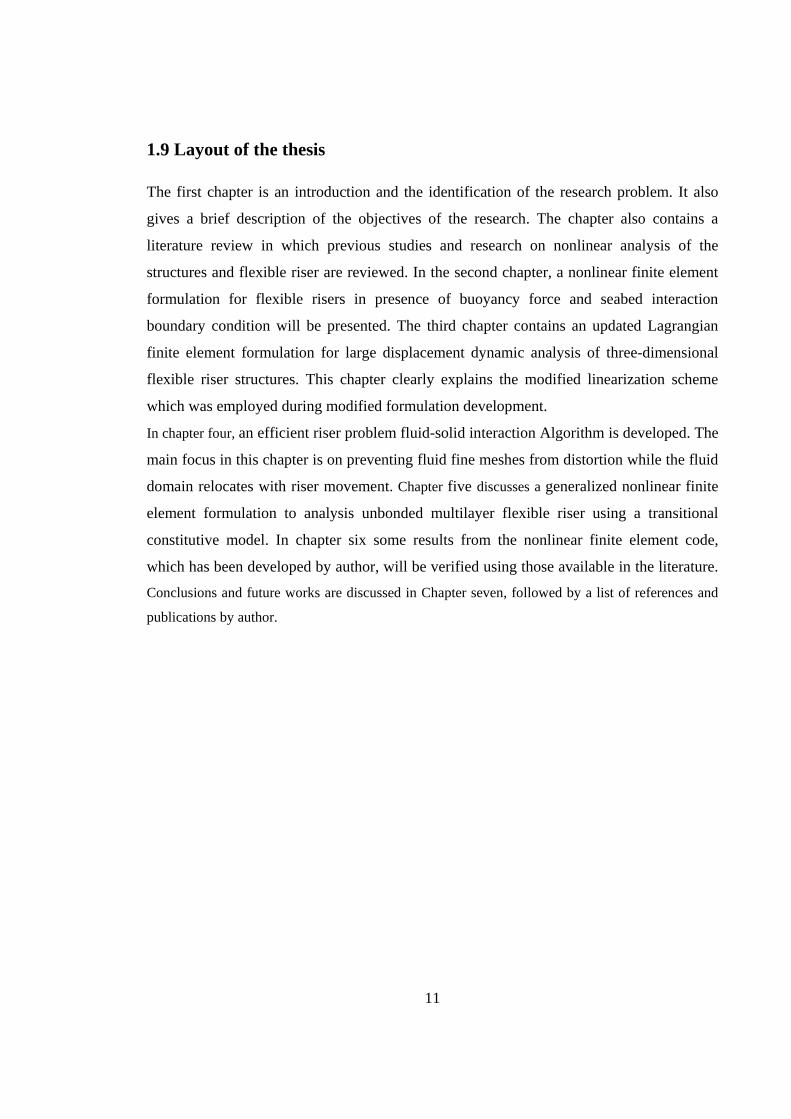
Figure 2.5: Large deformations for a body in a stationary Cartesian coordinate system

In the Lagrangian incremental analysis approach, the equilibrium of a deforming body at

time τ τ+Δ is expressed by using the principle of virtual displacements as follows [20]

ij ijV

e dVτ τ

τ τ τ τ τ ττ τσ δ

+Δ

+Δ +Δ +Δ+Δ = ℜ∫ (2.46)

where ijτ τσ+Δ are components of the Cauchy stress tensor and ijeτ τ+Δ are components of the

strain tensor. The left hand side of (2.46) is the virtual work performed when the body is

01 1 1, ,x x xτ τ τ+Δ

03 3 3, ,x x xτ τ τ+Δ

02 2 2, ,x x xτ τ τ+Δ

Configuration at time 0

Configuration at Time τ τ+Δ

0 A

Aτ

Configuration at time τ

Aτ τ+Δ

28

 

subjected to a virtual displacement at time τ τ+Δ . Also, τ τ+Δ ℜ is the external virtual work

expressed by

B Si i i i

V S

f u dV f u dSτ τ τ τ

τ τ τ τ τ τ τ τ τ τδ δ+Δ +Δ

+Δ +Δ +Δ +Δ +Δℜ= +∫ ∫ (2.47)

where Bif

τ τ+Δ and Sif

τ τ+Δ are components of the externally applied body and surface force

vectors respectively, and iuδ is the i th component of the virtual displacement vector.

The continuous change in the configuration of the body, when it undergoes large

deformations, entails some important consequences for the development of an incremental

analysis procedure. Since the configuration of the body at time τ τ+Δ is unknown, it is

difficult to apply Equation (2.46) in its general form. In addition, this change of

configuration is often accompanied by rigid body rotation of material particles and

the ijτ τσ+Δ components are affected by rigid body motions. Therefore, the Cauchy stresses

at time τ τ+Δ cannot be obtained by simply adding to the Cauchy stresses at time τ plus a

stress increment value, i.e. ij ij ijτ τ τ

τσ σ σ+Δ ≠ + .

In order to describe the equilibrium equation of the body correctly, suitable conjugate pair

of stress and strain tensors should be used [62]. There are various pairs of tensors that, in

principle, could be used for this purpose. In the present work, the 2nd Piola-Kirchhoff

stress tensor is used. This is defined by

, ,ij i m mn j nS x xτ

τ τ τ τ τ ττ τ τ τ ττ τ

ρ σρ

+Δ +Δ+Δ +Δ+Δ= (2.48)

29

 

where ,i m i mx x xτ τ τ ττ τ

+Δ+Δ =∂ ∂ , and τ τ τρ ρ+Δ represent the ratio of the mass densities at

time τ and timeτ τ+Δ . The 2nd Piola-Kirchhoff stress and the Green-Lagrange strain

tensors are energy conjugates [20, 62]. Therefore, for the present finite element formulation

the Green-Lagrange strain tensor is used as

( ), , , ,12ij i j j i k i k ju u u uτ τ τ τ τ τ τ τ τ τ

τ τ τ τ τε+Δ +Δ +Δ +Δ +Δ= + + (2.49)

The 2nd Piola-Kirchhoff stress and the Green-Lagrange strain are Lagrangian tensors that

are not affected by rigid body rotations. Thus, these two tensors are used to describe the

equilibrium equation of the body independent of rigid rotations. It is also recognised that

the 2nd Piola-Kirchhoff stress tensor has a little physical meaning and in practice the

Cauchy stress values are calculated in each increment and then using Equation (2.48) the

incremental values for 2nd Piola-Kirchhoff stress tensor determined.

2.7 Updated Lagrangian formulation

In large deformation analysis, the incremental form of the equilibrium equation has to be

derived in order to solve the nonlinear equations. For this purpose, we can employ Equation

(2.46) to refer the stresses and strains to one of the known equilibrium configurations. In

theory, any one of the already calculated equilibrium configurations could be used. Yet in

practice, the total Lagrangian (TL) or updated Lagrangian (UL) formulations are used. In

the total Lagrangian formulation all static and kinematic variables are referred to the initial

configuration at time 0 . But in updated Lagrangian formulation all variables are referred to

the configuration at time t . Both these formulations include all kinematic nonlinear effects

due to large displacements, large rotations and large strains. The only advantage of using

one formulation rather than the other lies in its greater numerical efficiency. However, in

30

 

practice, the updated Lagrangian approach requires less numerical effort. Thus, it is more

computationally efficient.

Using the 2nd Piola-Kirchhoff stress and the Green-Lagrange strain tensors in Equation

(2.46) together with an updated Lagrangian description, we obtain the incremental equation

of motion as follows

ij ijV

S dVτ

τ τ τ τ τ τ ττ τδ ε+Δ +Δ +Δ= ℜ∫ (2.50)

2.8 Linearization of updated Lagrangian formulation for incremental

solution

While the current configuration is unknown, Equation (2.50) is strongly nonlinear and in

order to obtain an incremental solution, the equation has to be modified to a linearized

form. Some linearization techniques proposed by other researchers can be found in the

literature [18, 20, 21, 63]. In order to proceed using an incremental scheme, incremental

decompositions of stresses and strains have to be used in the following forms

ij ij ijS Sτ τ ττ τσ+Δ = + (2.51)

,ij ij ij ij ijeτ ττ τ τ τ τε ε ε η+Δ = = + (2.52)

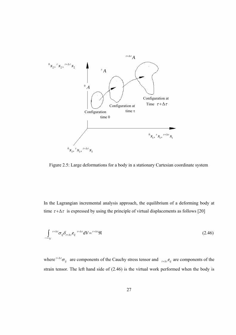
31

 

where ij ijSτ ττ σ= , ijeτ and ijτη stand for the linear and nonlinear parts of the incremental

strain components respectively. At the incremental level a constitutive equation of the form

ij ijrs rsS C eτ τ= is used by Bathe [20], where ij ijeτ τδ ε δ= . Also, ijrsCτ are components of the

material property tensor at time t . Using (2.51) and (2.52), the equation of motion (2.50)

can be written as

tijrs rs ij ij ij ij ij

V V V

C e e dV dV e dVτ τ

τ τ τ τ τ τ ττ τ τ τ τδ σ δ η σ δ+Δ+ = ℜ−∫ ∫ ∫ (2.53)

The right hand side of (2.53) represents the “out-of-balance virtual work”. In order to

reduce the error of the solution, an iterative procedure is adopted in each increment. For

this purpose, using the modified Newton-Raphson iterative method to solve Equation

(2.53), the expression for this equation at iteration i is written as

( ) ( )

( )

i iijijrs rs ij ij

V Vi

ijijV

C e e dV dV

e dV

τ τ

τ

τ τ τττ τ τ

τ τ τ ττ

δ σ δ η

σ δ+Δ

+

= ℜ−

∫ ∫

∫ (2.54)

During this linearization process a significant loss occurs in accuracy of the Lagrangian

formulation [18, 57, 63]. In this work and in Chapter 3 a particular linearization scheme is

also proposed to avoid such inaccuracies.

 

 

32

 

2.9 Updated Lagrangian finite element formulation

Using Equation (2.54), the incremental finite element equation of equilibrium can be

written as

( ) ( ) ( 1)( 1)

)(i ii i

L NLτ τ τ τ τ τ τ ττ τ τ τ τ τ

−−+Δ +Δ +Δ +Δ+Δ +Δ +Δ+ = −ΔK K U R F (2.55)

where ττ LK and τ

τ NLK are the linear and nonlinear (due to large deformation) stiffness

matrices and ( 1)iτ τ τ ττ τ

+Δ +Δ −+Δ−R F is the incremental load from time t toτ τ+Δ . Also, R

denotes the external load vector and F is the internal force vector. These matrices and

vectors are obtained based on equilibrium Equation (2.54) as follow

V

dVτ

τ τ τ ττ τ τ τ= ∫ T

L L LK B C B (2.56)

T

VNL NL NL d V

τ τ

τ τ τ τ τ τ τ τ τ ττ τ τ τ τ τ

+Δ

+Δ +Δ +Δ +Δ +Δ+Δ +Δ +Δ= ∫Κ B σ B (2.57)

TL

V

d Vτ τ

τ τ τ τ τ τ τ ττ τ τ τ

+Δ

+Δ +Δ +Δ +Δ+Δ +Δ= ∫F B σ) (2.58)

0 0

0 00 0

V S

dV dSτ τ τ τ τ τ+Δ +Δ +Δ= +∫ ∫T B ST SR H f H f (2.59)

33

 

Figure 2.6: Newton-Cotes formula’s integration point positions

In this work to evaluate these stiffness matrices and internal force vector, a reduced

numerical integration scheme using Newton-Cotes formula with the following orders is

employed; 3-point integration through the wall thickness, 5-point integration along the

length and 8-point integration around the circumference. Figure 2.6 shows the positions of

these integral points.

2.10 Buoyancy force

The buoyancy force is equal to the weight of the displaced fluid and acts on floating riser in

vertical direction opposite to the body force. Using this definition the following relation is

developed to estimate the buoyancy force vector, Buyτ τ+Δ R , consistent with the presented

flexible riser finite element formulation.

TBuy a Buy

l

d sτ τ

τ τ τ τ τ τ τ ττ τ

+Δ

+Δ +Δ +Δ +Δ+Δ= ∫R H q (2.60)

34

 

where

( )1...4

kBuy Buy k

τ τ τ τ+Δ +Δ

=⎡ ⎤= ⎣ ⎦q qL L (2.61)

and

( )

( )10

, 0, 01

0 0

0 0kBuy

w wr s t

V

ad V drl lτ τ

τ τ

τ τ τ ττ τ τ τ

ρ ρ+Δ

+Δ

+Δ +Δ= =+Δ +Δ −

⎧ ⎫ ⎧ ⎫⎪ ⎪ ⎪ ⎪⎪ ⎪ ⎪ ⎪⎪ ⎪ ⎪ ⎪= =⎨ ⎬ ⎨ ⎬⎪ ⎪ ⎪ ⎪⎪ ⎪ ⎪ ⎪

⎪ ⎪⎪ ⎪ ⎩ ⎭⎩ ⎭∫ ∫

q

J)

)

(2.62)

Therefore

( )1 T

, 0, 01Buy a Buy r s t drτ τ τ τ τ τ τ ττ τ

+Δ +Δ +Δ +Δ+Δ = =−

=∫R H q J (2.63)

In Equation (2.62), wρ is water density, lτ τ+Δ stands for the element length at τ τ+Δ and

Vτ τ+Δ ) is displaced water volume. Also, 0a is defined as

( )( )20 1 /i oa r rπ= − (2.64)

35

 

2.11 Steady state current loading

A displacement-dependent (follower) external load due to steady state current can be

expressed as

TCurrent a Current

l

d sτ τ

τ τ τ τ τ τ τ ττ τ

+Δ

+Δ +Δ +Δ +Δ+Δ= ∫R H q (2.65)

where

( )1...4

kCurrent Current k

τ τ τ τ+Δ +Δ

=⎡ ⎤= ⎣ ⎦q qL L (2.66)

qcurrent is the steady-state current force due to fluid-structure interaction (using Morison’s

equation) which can be decomposed into two vectors: transverse drag load vector and skin

friction or tangential drag vector. The transverse drag load vector per unit length is given

by:

( ) 12

kw Dn cn cnDn DC

lτ τ τ τ τ τ

τ τ ρ+Δ +Δ +Δ+Δ=q V V

r r (2.67)

and skin friction or tangential drag vector per unit length is defined as:

36

 

( ) 12

kw Dt ct ctDt D C

lτ τ τ τ τ τ

τ τ ρ+Δ +Δ +Δ+Δ=q V V

r r (2.68)

DnC and DtC are drag coefficients which are obtained from experiments and are functions

of Reynolds number of the current. cVr

is steady state current velocity vector.

( )cn c ctτ τ τ τ+Δ +Δ= −V V V

r r r and ( ( ) )T

ct c r rτ τ τ τ τ τ+Δ +Δ +Δ=V V V V

r r are normal and tangential

components of cVr

which are acting on the riser at time increment τ τ+Δ . Using Equations

(2.67) and (2.68) and assuming a uniform variation of current velocity with respect to water

depth results in

( ) ( ) ( )1 1

2 2

3 3

2

Dn cn cn Dt ct ctk k k w

Current Dn Dt Dn cn cn Dt ct ct

Dn cn cn Dt ct ct

C V C VD C V C V

lC V C V

τ τ τ τ τ τ τ τ

τ τ τ τ τ τ τ τ τ τ τ τ τ ττ τ

τ τ τ τ τ τ τ τ

ρ+Δ +Δ +Δ +Δ

+Δ +Δ +Δ +Δ +Δ +Δ +Δ+Δ

+Δ +Δ +Δ +Δ

⎧ ⎫+⎪ ⎪

= + = +⎨ ⎬⎪ ⎪+⎩ ⎭

V Vq q q V V

V V

r r

r r

r r (2.69)

Therefore

( )1 T

, 0, 01Current a Current r s t drτ τ τ τ τ τ τ ττ τ

+Δ +Δ +Δ +Δ+Δ = =−

=∫R H q J (2.70)

2.12 Seabed soil-riser interaction modeling

The pipe-soil interaction model (Figure 2.7) adopted in this study has been proposed by

Laver et. al. [60]. This model is based on some experiments which were conducted to

investigate the effects of pull-out rate, pipe diameter, consolidation time and consolidation

load.

37

 

 

 

Max. Uplift resistance force; Q

0.075

S, Max

Pipe displacement (m)

Break out displacement, 0.7

Uplift resistance force (kN)

Figure 2.7: Pipe-soil interaction model

The model profile has three linear phases as shown in Figure 2.7. From this figure, when

the pipe initially moves upwards the suction force ( sQ ) increases from zero to the

maximum value then the suction force remains constant as the pipe moves further upwards

finally under further upward movement the suction force reduces from its maximum value

to zero at the break-out displacement. The soil suction model has two defined limits the

maximum uplift resistance force per unit length, QS,MAX, and the break-out displacement, ΔB

which are estimated using the formulas below [60]

 

sQ (Uplift resident  

        force per unit length) 

38

 

, 20.00033 0.9Fn

p C VS MAX c F U

V F c tQ k k N D S

D LD

⎛ ⎞⎛ ⎞= +⎜ ⎟⎜ ⎟ ⎜ ⎟⎝ ⎠ ⎝ ⎠

(2.71)

20.0009 0.8D C VnB D p

F c tk V D

LD

⎛ ⎞Δ = +⎜ ⎟⎜ ⎟

⎝ ⎠ (2.72)

where ck is cyclic loading factor (=1.0 for slow drift motion) and Fk , Fn , Dk and Dn are

empirically derived constants; for onsoy clay 1.12, 0.18, 0.98F F Dk n k= = = , 0.26Dn = and

for watchet clay 0.98, 0.21, 0.83, 0.19F F D Dk n k n= = = = . Also, V is pull-out velocity

(between 0.005-0.2 m/s), D is external diameter of riser, CF is consolidation force (N), Vc

is coefficient of consolidation (m2/year), t is the consolidation time (years) and uS is un-

drained shear strength of soil. In Equation (2.71) Min[5.14 1.18 / ,7.5]N z B= + where z is

depth of riser invert and B is its bearing width. The bearing width of a pipe is typically

equal to its external diameter ( B D= ), but for the pipe penetration depth less than 12 D ,

22B Dz z= − . In this paper, in the large deformation finite-element context the seabed

interaction is applied as a follower external load. For this purpose for those elements with

seabed interaction and initial penetration, a force vector at each time step of incremental

solution is defined as

TLBed Bed

L

d Lτ τ

τ τ τ τ τ τ τ ττ τ τ τ

+Δ

+Δ +Δ +Δ +Δ+Δ +Δ= ∫R H q

)

) (2.73)

where

39

 

.

.

.

s z rl

Bed s z sl

s z tl

Q d l

Q d l

Q d l

τ τ

τ τ

τ τ

τ τ τ τ

τ τ τ τ τ τ

τ τ τ τ

+Δ

+Δ

+Δ

+Δ +Δ

+Δ +Δ +Δ

+Δ +Δ

⎧ ⎫⎪ ⎪⎪ ⎪⎪ ⎪=⎨ ⎬⎪ ⎪⎪ ⎪⎪ ⎪⎩ ⎭

∫

∫

∫

e V

q e V

e V

)

)

)

)

)

)

(2.74)

where l)

is length of those part of element which has interaction with seabed.

2.13 Solution Algorithm

The nonlinear finite element formulation derived in the previous sections has been coded in

a finite element program using an appropriate algorithm; Figure 2.8 gives an overview of

this algorithm. In this algorithm the outer loop carries out the incremental solution of the

problem and the external load vector is calculated in each increment. This figure illustrates

that in order to achieve convergence in each increment an iterative solution procedure has

to be employed in which in all iterations the stiffness matrices as well as the nodal force

vector should be updated for all integration points of every element. After calculating the

assembled global stiffness matrix and nodal force vector of the structure, the incremental

displacement vector will be calculated. In the next step, the geometry of the structure will

be updated using calculated incremental displacement values. Then, the stress and strain

tensors will be calculated for all integration points. These iterative solutions will continue

until the convergence criterion is satisfied.

40

 

Figure 2.8: Nonlinear solution algorithm

41

Chapter 3

An Updated Lagrangian Finite Element

Formulation for Large Displacement Dynamic

Analysis of Three-Dimensional Flexible Riser

Structures

3.1 Introduction

The finite element formulation that was presented in Chapter 2 can be used for modeling

large rigid body motion, large displacement with small rotations. In a case problem with

large rotation, due to some singularity in rotational degrees of freedom the formulation fails

to model finite deformation [15, 57]. In this chapter, an updated Lagrangian finite element

formulation of a three-dimensional annular section flexible riser element is presented for

large displacement and large rotation dynamic analysis of flexible riser structures. In this

formulation a modified linearization method is used to avoid inaccuracies normally

associated with other linearization schemes.

42

3.2 Kinematics of three-dimensional riser element The element employed in the present chapter is the same four-nodded, twenty four degrees

of freedom flexible riser element Figure 2.1. This element is a continuum based element

whose displacement field at time τ τ+ Δ is obtained as

4 4 4

1 1 1( , , ) ( ) ( ) ( ) ; 1, 2,3k k k k k

i k i k ti k sik k k

r s t r r ru h u t a h V s a h V iτ τ τ τ+Δ +Δ

= = == + + =∑ ∑ ∑ (3.1)

where all parameters in this equation were defined in Chapter 2.

3.3 An incremental solution for flexible riser element using a novel

linearization approach According to detail explanations from Chapter 2, in the UL incremental analysis approach,

the equilibrium equations of a deforming body at time τ τ+ Δ are expressed using the

principle of virtual displacements as:

( )ij ijV

S E dVτ

τ τ τ τ τ ττ τ τδ+Δ +Δ +Δ= ℜ∫ % (3.2)

where ijSτ ττ

+Δ is the 2nd Piola-Kirchhoff stress, ijEτ ττ

+Δ is the Green-Lagrange strain and

parameter τ ττ

+Δ ℜ% represents the external virtual work. An expression for τ ττ

+Δ ℜ% includes

all external loadings applied to the body (flexible riser) such as current loading, buoyancy

force as well as inertia force. Writing (3.2) for dynamic analysis of body by excluding

inertia force from τ ττ

+Δ ℜ% results in:

( )i i ij ijV V

u u dV S E dVτ τ τ

τ τ τ τ τ τ τ ττ τ τρ δ δ

+Δ

+Δ +Δ +Δ +Δ+ = ℜ∫ ∫&& (3.3)

43

In Equation (3.3) the 2nd Piola-Kirchhoff stress and Green-Lagrange strain tensors are an

energy conjugate pair [62], both of which are unaffected by rigid body rotations. The

incremental form of the Green-Lagrange strain tensor is as follows:

( ), , , ,12ij i j j i k i k jE u u u uτ τ τ τ τ τ τ τ τ τ

τ τ τ τ τ+Δ +Δ +Δ +Δ +Δ= + + (3.4)

Also, the relation between the 2nd Piola-Kirchhoff stress components ijS and the Cauchy

stress components mnσ is written as follows:

( ), , ,detmn m i m i ij n jx x S xτ τ τ τ τ τ τ τ τ ττ τ τ τσ+Δ +Δ +Δ +Δ +Δ= (3.5)

where , /m i m ix x xτ τ τ τ ττ

+Δ +Δ=∂ ∂ represents the deformation gradient of the increment.

Substitution of displacement field (3.1) into Equation (3.4) yields a second order function

for expressing the Green-Lagrange strain tensor as follows [57]

(0) (1) (2)

(3) 2 (4) 2 (5)( , , ) ( ) ( ) ( )

( ) ( ) ( )ij ij ij ij

ij ij ij

E r s t E r s E r t E rst E r s E r t E r

τ τ τ τ τ τ τ ττ τ τ τ

τ τ τ τ τ ττ τ τ

+Δ +Δ +Δ +Δ

+Δ +Δ +Δ

= + +

+ + + (3.6)

where

4 4 4 4 4(0) 1 1 1 1 1

1 , 2 3 1 , 21 1 1 1 1

4 4 4 41 1 1 1

3 1 , 2 31 1 1 1

11 ,

2 k k k k k k k k k k k k kij j r i j si j ti i r j i sj

k k k k k

k k k k k k k k k k ki tj i r k i sk i tk

k k k k

kj r

E J h u J h a V J h a V J h u J h a V

J h a V J h u J h a V J h a V

J h

τ τ τ ττ

τ

τ

+Δ − − − − −

= = = = =

− − − −

= = = =

−

= + + + +

⎛ ⎞+ + + +⎜ ⎟

⎝ ⎠

×

∑ ∑ ∑ ∑ ∑

∑ ∑ ∑ ∑4 4 4

1 12 3

1 1 1

k k k k k k kk j sk j tk

k k ku J h a V J h a V− −

= = =

⎛ ⎞+ +⎜ ⎟

⎝ ⎠∑ ∑ ∑

(3.7)

44

4 4(1) 1 1

1 , 1 ,1 1

4 4 4 41 1 1 1

1 , 2 3 1 ,1 1 1 1

4 41 1 1

1 , 1 , 21 1

2 k k k k k kij j r si i r sj

k k

k k k k k k k k k k ki r k i sk i tk j r sk

k k k k

k k k k k k ki r sk j r k j

k k

E J h a V J h a V

J h u J h a V J h a V J h a V

J h a V J h u J h a

τ ττ

τ

τ

+Δ − −

= =

− − − −

= = = =

− − −

= =

= +

⎛ ⎞ ⎛ ⎞+ + + ×⎜ ⎟ ⎜ ⎟⎝ ⎠ ⎝ ⎠⎛ ⎞

+ × +⎜ ⎟⎝ ⎠

∑ ∑

∑ ∑ ∑ ∑

∑ ∑4 4

13

1 1

k k k ksk j tk

k kV J h a V−

= =

⎛ ⎞+⎜ ⎟

⎝ ⎠∑ ∑

(3.8)

4 4(2) 1 1

1 , 1 ,1 1

4 4 4 41 1 1 1

1 , 2 3 1 ,1 1 1 1

4 41 1 1

1 , 1 , 21 1

2 k k k k k kij j r ti i r tj

k k

k k k k k k k k k k ki r k i sk i tk j r tk

k k k k

k k k k k k ki r tk j r k j

k k

E J h a V J h a V

J h u J h a V J h a V J h a V

J h a V J h u J h a

τ ττ

τ

τ

+Δ − −

= =

− − − −

= = = =

− − −

= =

= +

⎛ ⎞ ⎛ ⎞+ + + ×⎜ ⎟ ⎜ ⎟⎝ ⎠ ⎝ ⎠⎛ ⎞

+ × +⎜ ⎟⎝ ⎠

∑ ∑

∑ ∑ ∑ ∑

∑ ∑4 4

13

1 1

k k k ksk j tk

k kV J h a V−

= =

⎛ ⎞+⎜ ⎟

⎝ ⎠∑ ∑

(3.9)

4 4(3) 1 1

1 , 1 ,1 1

k k k k k k k kij i r sk tk j r sk tk

k kE J h a V V J h a V Vτ τ

τ+Δ − −

= == ×∑ ∑

(3.10)

4 4(4) 1 1

1 , 1 ,1 1

12

k k k k k kij i r sk j r sk

k kE J h a V J h a Vτ τ

τ+Δ − −

= =

= ×∑ ∑ (3.11)

4 4(5) 1 1

1 , 1 ,1 1

12

k k k k k kij i r tk j r tk

k kE J h a V J h a Vτ τ

τ+Δ − −

= =

= ×∑ ∑ (3.12)

mnJ are the Jacobian matrix components referred to configuration at time τ. Using

Equation (3.6) together with stress-strain relation ij ijkl klS C Eτ τ τ τ τ ττ τ τ

+Δ +Δ +Δ= , the 2nd Piola-

Kirchhoff stress tensor can be written as

45

(0) (1) (2)

(3) 2 (4) 2 (5)( , , ) ( ) ( ) ( )

( ) ( ) ( )ij ij ij ij

ij ij ij

S r s t S r s S r t S rst S r s S r t S r

τ τ τ τ τ τ τ ττ τ τ τ

τ τ τ τ τ ττ τ τ

+Δ +Δ +Δ +Δ

+Δ +Δ +Δ

= + +

+ + + (3.13)

where

( ) ( ) P( ) ( ) ; 0 5ij ijkl klS r C E rτ τ τ τ τ ττ τ τ

ΡΡ+Δ +Δ +Δ= = L (3.14)

Also, in view of Equation (3.14) and using Equation (3.5), the Cauchy stress components,

can be written as

( ) ( ) ( ), , ,( ) det ( ) ; 0 5mn m i m i ij n jr x x S r xτ τ τ τ τ τ τ τ τ τ

τ τ τ τσ Ρ Ρ+Δ +Δ +Δ +Δ +Δ= Ρ= L (3.15)

In order to develop an incremental solution for nonlinear Equation (3.2), the stress and

strain tensors are decomposed into:

ij ij ij ij ijS S S Sτ τ τ ττ σ+Δ = +Δ = +Δ (3.16)

ij ij ij ijE E eτ ττ η+Δ = Δ =Δ +Δ (3.17)

where operator Δ stands for the incremental values. The parameters ijeΔ and ijηΔ are the

linear and nonlinear parts of the incremental Green-Lagrange strain tensor and ijSΔ is the

incremental 2nd Piola-Kirchhoff stress tensor. Using Equations (3.13) and (3.16) we obtain

3 3

2 4 4 2 5 5

( ) ( ) ( ) ( )( ) ( )

ij ij ij ij ij ij ij ij ij

ij ij ij ij

S S s S t S st Ss S t S

τ τ τ τ τ ττ

τ τ

σ σ σ σσ σ

+Δ = +Δ + +Δ + +Δ + +Δ

+ +Δ + +Δ

(0) (0) (1) (1) (2) (2) ( ) ( )

( ) ( ) ( ) ( ) (3.18)

Substituting Equations (3.17) and (3.18) into nonlinear Equation (3.2) and after some

manipulation, the equilibrium equation of a deforming riser body at time τ τ+Δ is obtained

as

46

( )3 2 4 2 5

( )

( )

i i ij ijV V

ij ij ij ij ij ij ijV

u u dV S e dV

S s S t S st S s S t S dVτ τ τ

τ

τ τ

τ τ τ τ τ τ τ τ τ τ τ ττ τ τ τ τ τ

ρ δ δ

δ η+Δ

+Δ

+Δ +Δ +Δ +Δ +Δ +Δ

+ Δ

+ + + + + + Δ

∫ ∫

∫

(0)

(0) (1) (2) ( ) ( ) ( )

&&

( )3 2 4 2 5 ( )ij ij ij ij ij ij ijV

s S t S st S s S t S e dVτ

τ τ τ τ τ τ τ τ τ τ τ τ ττ τ τ τ τ τσ δ+Δ +Δ +Δ +Δ +Δ +Δ= ℜ− + + + + + Δ∫ (0) (1) (2) ( ) ( ) ( )

(3.19)

In Equation (3.19), the second term in the left hand side which is a nonlinear term, is

linearized using a Taylor series expansion as follows

{{

( )( ) ( ) ( )

( )

( )

( )

rs

ijrs

ijij ij rs rs ij

rsV V tNeglect Neglecte

ijrs rs ijV

C

SS e dV e highorder terms e dV

E

C e e dV

τ τ

τ

δ η δ

δ

↓ ↓ ↓≈Δ↓

∂Δ = Δ +Δ + Δ

∂

Δ Δ

∫ ∫

∫

(0)(0) (0) (0)

(0) 144244314243

(3.20)

Therefore, a linearized incremental virtual work equation is obtained in the form of

( )3 2 4 2 5

( )

( )

i i ijrs rs ijV V

ij ij ij ij ij ij ijV

u u dV C e e dV

S s S t S st S s S t S dVτ τ τ

τ

τ τ

τ τ τ τ τ τ τ τ τ τ τ ττ τ τ τ τ τ

ρ δ δ

δ η+Δ

+Δ

+Δ +Δ +Δ +Δ +Δ +Δ

+ Δ Δ Δ

+ + + + + + Δ

∫ ∫

∫ (0) (1) (2) ( ) ( ) ( )

&&

( )3 2 4 2 5 ( )ij ij ij ij ij ij ijV

s S t S st S s S t S e dVτ

τ τ τ τ τ τ τ τ τ τ τ τ ττ τ τ τ τσ δ+Δ +Δ +Δ +Δ +Δ +Δ= ℜ− + + + + + Δ∫ (0) (1) (2) ( ) ( ) ( )

(3.21)

The right hand side of Equation (3.21) is the out-of-balance virtual work. During the

numerical solution process, an iterative scheme is performed in each increment of the

solution based on the modified Newton-Raphson method to get the equilibrium state.

Hence, in iteration i Equation (3.21) is represented as:

47

( ) ( )

( ) ( ) ( ) ( ) ( ) ( )1 1 1 1 1 13 2 4 2 5

( )

( )

i i

i rsi ijrs ijV V

i i i i i i

ij ij ij ij ij ij ijV

u u dV C e e dV

S s S t S st S s S t S dV

τ τ τ

τ

τ τ

τ τ τ τ τ τ τ τ τ τ τ ττ τ τ τ τ τ

ρ δ δ

δ η

+Δ

+Δ

− − − − − −+Δ +Δ +Δ +Δ +Δ +Δ

+ Δ Δ Δ

⎛ ⎞⎜ ⎟+ + + + + + Δ⎜ ⎟⎝ ⎠

∫ ∫

∫ (0) (1) (2) ( ) ( ) ( )

&&

( ) ( ) ( ) ( ) ( ) ( )1 1 1 1 1 13 2 4 2 5 ( )

i i i i i i

ij ij ij ij ij ij ijV

s S t S st S s S t S e dVτ

τ τ τ τ τ τ τ τ τ τ τ τ ττ τ τ τ τσ δ

− − − − − −+Δ +Δ +Δ +Δ +Δ +Δ

⎛ ⎞⎜ ⎟= ℜ− + + + + + Δ⎜ ⎟⎝ ⎠∫ (0) (1) (2) ( ) ( ) ( )

(3.22)

3.4 Nonlinear Dynamic Finite Element Formulation for Flexible Riser

Structures Using Equation (3.22) a finite element formulation for geometrically nonlinear dynamic

analysis of riser structures is developed. The incremental form of this finite element

formulation for iteration i at time step τ+Δτ is

( ) ( ) ( ) ( )( 1) ( 1))(

ii i ii i

L NL

− −+ + = −U K K U R FM && (3.23)

Where M is time dependent mass matrix, LK and NLK are the linear and nonlinear (due to

large deformation) stiffness matrices. Also, R denotes the external load vector and F is the

internal force vector. These matrices and vector are obtained based on equilibrium Equation

(3.22), i.e.

T

V

dVτ τ

ρ+Δ

= ∫M H H (3.24)

T ( , , ) ( , , )L L LV

r s t r s t dVτ τ+Δ

= Δ∫Κ B CB (3.25)

48

( )T 3 2 4 2 5

V

( , , ) ( , , )NL

NL NLr s t r s ts t st s t dVτ τ

τ τ τ τ τ τ τ τ τ τ τ ττ τ τ τ τ τ

+Δ

+Δ +Δ +Δ +Δ +Δ +Δ

=

+ + + + +∫ (0) (1) (2) ( ) ( ) ( )Κ

B S S S S S S B

(3.26)

( )T 3 2 4 2 5( , , )LV

r s t s t st s t dVτ τ

τ τ τ τ τ τ τ τ τ τ ττ τ τ τ τ

+Δ

+Δ +Δ +Δ +Δ +Δ= + + + + +∫ (0) (1) (2) ( ) ( ) ( )F B σ S S S S S) ) ) ) )) (3.27)

where H is displacement interpolation matrix which is given in Equation (2-21), ΔC is the

incremental material properties matrix, S the 2nd Piola-Kirchhoff stress tensor, and S)

and

σ) are vectors containing the components of the 2nd Piola-Kirchhoff and Cauchy stress

tensors, respectively. It is noted that all these matrices and vectors are independent of the s

and t parameters. Also, H together with LB and NLB which are the linear and nonlinear

strain-displacement matrices, respectively, are the only s and t -dependent matrices which

can be decomposed as

( , , ) ( ) ( ) ( )r s t r r rs t= + +a b cH H H H (3.28)

( , , ) ( ) ( ) ( )L L L Lr s t r r rs t= + +a b cB B B B (3.29)

( , , ) ( ) ( ) ( )NL NL NL NLr s t r r rs t= + +a b cB B B B (3.30)

where the new matrices in Equations (3.28)-(3.30) are defined as follow

( )1...4

( ) ( )ka a

kr r

=⎡ ⎤=⎣ ⎦

H HL L , ( ) ( )

0 0 0 0 00 0 0 0 00 0 0 0 0

kk

a k

k

r

hh

h

⎡ ⎤⎢ ⎥=⎢ ⎥⎢ ⎥⎣ ⎦

H (3.31)

( )1...4

( ) ( )kb b

kr r

=

⎡ ⎤= ⎢ ⎥⎣ ⎦H HL L , ( )

3 2

3 1

2 1

( )

0 0 0 0

0 0 0 0

0 0 0 0

k ks s

k k kk k s sb

k ks s

r

V V

a h V V

V V

τ τ τ τ

τ τ τ τ

τ τ τ τ

+Δ +Δ

+Δ +Δ

+Δ +Δ

⎡ ⎤−⎢ ⎥

= −⎢ ⎥⎢ ⎥

−⎢ ⎥⎣ ⎦

H (3.32)

49

( )1...4

( ) ( )kc c

kr r

=⎡ ⎤=⎣ ⎦

H HL L , ( )3 2

3 1

2 1

( )

0 0 0 0

0 0 0 0

0 0 0 0

k kt t

k k kc k k t t

k kt t

r

V V

a h V V

V V

τ τ τ τ

τ τ τ τ

τ τ τ τ

+Δ +Δ

+Δ +Δ

+Δ +Δ

⎡ ⎤−⎢ ⎥

= − −⎢ ⎥⎢ ⎥

−⎢ ⎥⎣ ⎦

H (3.33)

( )1...4

( ) ( )kLa La

kr r

=

⎡ ⎤= ⎢ ⎥⎣ ⎦B BL L ,

( )

( ) ( ) ( )( ) ( ) ( )( ) ( ) ( )

( ) ( ) ( ) ( ) ( ) ( )( ) ( ) ( ) ( ) ( ) ( )( ) ( ) ( ) ( ) ( ) ( )

,1 11 11 11

,2 22 22 22

,3 33 33 33

,2 ,1 12 21 12 21 12 21

,3 ,2 23 32 23 32 23 32

,3 ,1 13 31 13 31 13 31

( )

0 0 1 2 3

0 0 1 2 3

0 0 1 2 3

0 1 1 2 2 3 3

0 1 1 2 2 3 3

0 1 1 2 2 3 3

k k kk

k k kk

k k kk k

La k k k k k kk k

k k k k k kk k

k k k k k kk k

r

h

h

h

h h

h h

h h

⎡ Φ Φ Φ⎢

Φ Φ Φ

Φ Φ Φ=

Φ + Φ Φ + Φ Φ + Φ

Φ + Φ Φ + Φ Φ + Φ

Φ + Φ Φ + Φ Φ + Φ⎣

B

⎤⎥

⎢ ⎥⎢ ⎥⎢ ⎥⎢ ⎥⎢ ⎥⎢ ⎥⎢ ⎥⎢ ⎥⎢ ⎥⎦

(3.34)

( )1...4

( ) ( )kLb Lb

kr r

=

⎡ ⎤= ⎢ ⎥⎣ ⎦B BL L ,

( )

( ) ( ) ( )( ) ( ) ( )( ) ( ) ( )

( ) ( ) ( ) ( ) ( ) ( )( ) ( ) ( ) ( ) ( ) ( )( ) ( ) ( ) ( ) ( ) ( )

11 11 11

22 22 22

33 33 33

12 21 12 21 12 21

23 32 23 32 23 32

13 31 13 31 13 31

( )

ˆ ˆ ˆ0 0 0 1 2 3

ˆ ˆ ˆ0 0 0 1 2 3

ˆ ˆ ˆ0 0 0 1 2 3

ˆ ˆ ˆ ˆ ˆ ˆ0 0 0 1 1 2 2 3 3

ˆ ˆ ˆ ˆ ˆ ˆ0 0 0 1 1 2 2 3 3

ˆ ˆ ˆ ˆ ˆ ˆ0 0 0 1 1 2 2 3 3

k k k

k k k

k k k

kLb k k k k k k

k k k k k k

k k k k k k

r

⎡ Φ Φ Φ⎢

Φ Φ Φ

Φ Φ Φ=

Φ + Φ Φ + Φ Φ + Φ

Φ + Φ Φ + Φ Φ + Φ

Φ + Φ Φ + Φ Φ + Φ⎣

B

⎤⎥

⎢ ⎥⎢ ⎥⎢ ⎥⎢ ⎥⎢ ⎥⎢ ⎥⎢ ⎥⎢ ⎥⎢ ⎥⎢ ⎥⎢ ⎥⎦

(3.35)

( )1...4

( ) ( )kLc Lc

kr r

=

⎡ ⎤= ⎢ ⎥⎣ ⎦B BL L ,

50

( )

( ) ( ) ( )( ) ( ) ( )( ) ( ) ( )

( ) ( ) ( ) ( ) ( ) ( )( ) ( ) ( ) ( ) ( ) ( )( ) ( ) ( ) ( ) ( ) ( )

11 11 11

22 22 22

33 33 33

12 21 12 21 12 21

23 32 23 32 23 32

13 31 13 31 13 31

( )

0 0 0 1 2 3

0 0 0 1 2 3

0 0 0 1 2 3

0 0 0 1 1 2 2 3 3

0 0 0 1 1 2 2 3 3

0 0 0 1 1 2 2 3 3

k k k

k k k

k k kk

Lc k k k k k k

k k k k k k

k k k k k k

r

⎡ ⎤Φ Φ Φ⎢ ⎥⎢ ⎥Φ Φ Φ⎢ ⎥⎢ ⎥Φ Φ Φ=⎢ ⎥

Φ + Φ Φ + Φ Φ + Φ⎢ ⎥⎢ ⎥

Φ + Φ Φ + Φ Φ + Φ⎢ ⎥⎢ ⎥

Φ + Φ Φ + Φ Φ + Φ⎢ ⎥⎣ ⎦

B (3.36)

( )1...4

( ) ( )kNLa NLa

kr r

=

⎡ ⎤= ⎢ ⎥⎣ ⎦B BL L , ( )

( ) ( ) ( )( ) ( ) ( )( ) ( ) ( )( ) ( ) ( )( ) ( ) ( )( ) ( ) ( )( ) ( ) ( )( ) ( ) ( )( ) ( ) ( )

,1 11 11 11

,2 12 12 12

,3 13 13 13

,1 21 21 21

,2 22 22 22

,3 23 23 23

,1 31 31 31

,2 32 32 32

,3 33 33 33

( )

0 0 1 2 3

0 0 1 2 3

0 0 1 2 3

0 0 1 2 3

0 0 1 2 3

0 0 1 2 3

0 0 1 2 3

0 0 1 2 3

0 0 1 2 3

k k kk

k k kk

k k kk

k k kk

k k k kNLa k

k k kk

k k kk

k k kk

k k kk

r

h

h

h

h

h

h

h

h

h

⎡ Φ Φ Φ

Φ Φ Φ

Φ Φ Φ

Φ Φ Φ

= Φ Φ Φ

Φ Φ Φ

Φ Φ Φ

Φ Φ Φ

Φ Φ Φ⎣

B

⎤⎢ ⎥⎢ ⎥⎢ ⎥⎢ ⎥⎢ ⎥⎢ ⎥⎢ ⎥⎢ ⎥⎢ ⎥⎢ ⎥⎢ ⎥⎢ ⎥⎢ ⎥⎢ ⎥⎢ ⎥⎦

(3.37)

( )1...4

( ) ( )kNLb NLb

kr r

=

⎡ ⎤=⎢ ⎥⎣ ⎦B BL L , ( )

( ) ( ) ( )( ) ( ) ( )( ) ( ) ( )( ) ( ) ( )( ) ( ) ( )( ) ( ) ( )( ) ( ) ( )( ) ( ) ( )( ) ( ) ( )

11 11 11

12 12 12

13 13 13

21 21 21

22 22 22

23 23 23

31 31 31

32 32 32

33 33 33

( )

ˆ ˆ ˆ0 0 0 1 2 3

ˆ ˆ ˆ0 0 0 1 2 3

ˆ ˆ ˆ0 0 0 1 2 3

ˆ ˆ ˆ0 0 0 1 2 3

ˆ ˆ ˆ0 0 0 1 2 3

ˆ ˆ ˆ0 0 0 1 2 3

ˆ ˆ ˆ0 0 0 1 2 3

ˆ ˆ ˆ0 0 0 1 2 3

ˆ ˆ ˆ0 0 0 1 2 3

k k k

k k k

k k k

k k k

k k kkNLb

k k k

k k k

k k k

k k k

r

⎡ Φ Φ Φ

Φ Φ Φ

Φ Φ Φ

Φ Φ Φ

= Φ Φ Φ

Φ Φ Φ

Φ Φ Φ

Φ Φ Φ

Φ Φ Φ⎣

B

⎤⎢ ⎥⎢ ⎥⎢ ⎥⎢ ⎥⎢ ⎥⎢ ⎥⎢ ⎥⎢ ⎥⎢ ⎥⎢ ⎥⎢ ⎥⎢ ⎥⎢ ⎥⎢ ⎥⎢ ⎥⎢ ⎥⎢ ⎥⎢ ⎥⎢ ⎥⎦

(3.38)

51

( )1...4

( ) ( )kNLc NLc

kr r

=

⎡ ⎤=⎢ ⎥⎣ ⎦B BL L , ( )

( ) ( ) ( )( ) ( ) ( )( ) ( ) ( )( ) ( ) ( )( ) ( ) ( )( ) ( ) ( )( ) ( ) ( )( ) ( ) ( )( ) ( ) ( )

11 11 11

12 12 12

13 13 13

21 21 21

22 22 22

23 23 23

31 31 31

32 32 32

33 33 33

( )

0 0 0 1 2 3

0 0 0 1 2 3

0 0 0 1 2 3

0 0 0 1 2 3

0 0 0 1 2 3

0 0 0 1 2 3

0 0 0 1 2 3

0 0 0 1 2 3

0 0 0 1 2 3

k k k

k k k

k k k

k k k

k k kkNLc

k k k

k k k

k k k

k k k

r

⎡ ⎤Φ Φ Φ⎢ ⎥⎢ ⎥Φ Φ Φ⎢ ⎥⎢ ⎥Φ Φ Φ⎢ ⎥⎢ ⎥Φ Φ Φ⎢ ⎥⎢ ⎥= Φ Φ Φ⎢⎢ Φ Φ Φ⎢⎢ Φ Φ Φ⎢⎢ Φ Φ Φ⎢⎢ Φ Φ Φ⎢⎣ ⎦

B⎥⎥⎥⎥⎥⎥⎥⎥⎥

(3.39)

in Equations (3.34)-(3.39), parameters ( )km in

Φ , ( )ˆ k

m inΦ and ( )k

m inΦ are defined as follow

( ) ( ) ( )1 12 3

ˆ k kkm n n kin mimi

J J hφ φ− −⎛ ⎞Φ = +⎜ ⎟⎝ ⎠

(3.40)

( ) ( )11

ˆˆ kk km nin mi

hJr

φ− ∂⎛ ⎞Φ =⎜ ⎟ ∂⎝ ⎠ (3.41)

( ) ( )( )11

kk km nin mi

hJr

φ− ∂Φ =

∂ (3.42)

where, nonzero values for φ̂ and φ are

( ) ( ) 312 21ˆ ˆ 0.5

k k k ksa Vτ τφ φ +Δ=− =− (3.43)

( ) ( ) 213 31ˆ ˆ 0.5

k k k ksa Vτ τφ φ +Δ=− = (3.44)

52

( ) ( ) 123 32ˆ ˆ 0.5

k k k ksa Vτ τφ φ +Δ=− =− (3.45)

( ) ( ) 312 210.5

k k k kta Vτ τφ φ +Δ=− =− (3.46)

( ) ( ) 213 310.5

k k k kta Vτ τφ φ +Δ=− = (3.47)

( ) ( ) 123 320.5

k k k kta Vτ τφ φ +Δ=− =− (3.48)

Now, substitution of Equations (3.28)-(3.30) into Equations (3.24)-(3.27) results in

( )2 2( ) ( ) ( ) ( ) ( ) ( )a b c d e fV

r s r t r st r s r t r dVτ τ

ρ+Δ

+ + + + += ∫M M M M M M M (3.49)

( )2 2( ) ( ) ( ) ( ) ( ) ( )L La Lb Lc Ld Le LfV

r s r t r st r s r t r dVτ τ+Δ

+ + + + += ∫Κ Κ Κ Κ Κ Κ Κ (3.50)

(

)

2 2

2 2 3 3 2 2

3 3 4 4

( ) ( ) ( ) ( ) ( ) ( )

( ) ( ) ( ) ( ) ( )

( ) ( ) ( ) ( )

NL NLa NLb NLc NLd NLe NLfV

NLg NLh NLi NLj NLk

NLl NLm NLn NLo

r s r t r st r s r t r

s r st r s r t r s t r

s r st r s r t r

t

t dV

τ τ+Δ

+ + + + +

+ + + + +

+ + + +

= ∫Κ Κ Κ Κ Κ Κ Κ

Κ Κ Κ Κ Κ

Κ Κ Κ Κ

(3.51)

()

2 2

2 2 3 3

( ) ( ) ( ) ( ) ( ) ( )

( ) ( ) ( ) ( )

a b c d e fV

g h i j

r s r t r st r s r t r

s r st r s r t rt dVτ τ+Δ

+ + + + +

+ + + +

= ∫F F F F F F F

F F F F (3.52)

the new matrices and vectors in these equations are defined as follows

T( )a a ar =M H H (3.53)

53

T T( )b a b b ar = +M H H H H (3.54)

T T( )c a c c ar = +M H H H H (3.55)

T T( )d b c c br = +M H H H H (3.56)

T( )e b br =M H H (3.57)

T( )f c cr =M H H (3.58)

T( )La La Lar =Κ B CB (3.59)

T T( )Lb La Lb Lb Lar = +Κ B CB B CB (3.60)

T T( )Lc La Lc Lc Lar = +Κ B CB B CB (3.61)

T T( )Ld Lb Lc Lc Lbr = +Κ B CB B CB (3.62)

T( )Le Lb Lbr =Κ B CB (3.63)

T( )Lf Lc Lcr =Κ B CB (3.64)

T (0)( )NLa NLa NLar =Κ B S B (3.65)

T (1) T (0) T (0)( ) + +NLb NLa NLa NLb NLa NLa NLbr =Κ B S B B S B B S B (3.66)

T (2) T (0) T (0)( ) + +NLc NLa NLa NLc NLa NLa NLcr =Κ B S B B S B B S B (3.67)

54

T (1) T (2) T (0) T (0)

T (1) T (3) T (2)( ) + + +

+ + +NLd NLa NLc NLa NLb NLb NLc NLc NLb

NLc NLa NLa NLa NLb NLa

r =Κ B S B B S B B S B B S BB S B B S B B S B

(3.68)

T (0) T (4) T (1) T (1)( ) + + +NLe NLb NLb NLa NLa NLb NLa NLa NLbr =Κ B S B B S B B S B B S B (3.69)

T (2) T (0) T (5) T (2)( ) + + +NLf NLa NLc NLc NLc NLa NLa NLc NLar =Κ B S B B S B B S B B S B (3.70)

T (3) T (4) T (1) T (2)

T (1) T (4) T (3)( ) + + +

+ + +NLg NLa NLb NLa NLc NLb NLc NLb NLb

NLc NLb NLc NLa NLb NLa

r =Κ B S B B S B B S B B S BB S B B S B B S B

(3.71)

T (3) T (5) T (2) T (1)

T (2) T (5) T (3)( ) + + +

+ + +NLh NLa NLc NLa NLb NLb NLc NLc NLc

NLc NLb NLb NLa NLc NLa

r =Κ B S B B S B B S B B S BB S B B S B B S B

(3.72)

T (4) T (1) T (4)( ) + +NLi NLa NLb NLb NLb NLb NLar =Κ B S B B S B B S B (3.73)

T (5) T (2) T (5)( ) + +NLj NLa NLc NLc NLc NLc NLar =Κ B S B B S B B S B (3.74)

T (3) T (5) T (3) T (4)( )= + + +NLk NLb NLc NLb NLb NLc NLb NLc NLcrΚ B S B B S B B S B B S B (3.75)

T (3) T (4) T (4)( ) + +NLl NLb NLb NLb NLc NLc NLbr =Κ B S B B S B B S B (3.76)

T (5) T (3) T (5)( ) + +NLm NLb NLc NLc NLc NLc NLbr =Κ B S B B S B B S B (3.77)

T (4)( )NLn NLb NLbr =Κ B S B (3.78)

T (5)( )NLo NLc NLcr =Κ B S B (3.79)

55

Equations (3.49)-(3.52) can be evaluated by a selected order of Gaussian quadrature

numerical integration procedure over the annular section riser element volume. In order to

make the formulation more efficient and to avoid higher order numerical integrations, and

since some of the terms in Equations (3.49)-(3.52) are eliminated, an analytical integration

scheme for through-the-thickness coordinates r and t is employed for solution of these

equations. Thus, after explicitly integrating Equations (3.49)-(3.52), we get:

( ) ( )1

0 1 , 0, 01( ) ( ) ( )a e f r s tr r ra a drρ = =−

+ +⎡ ⎤= ⎣ ⎦∫M M M M J (3.80)

( ) ( )1

0 1 , 0, 01( ) ( ) ( )L La Le Lf r s tr r ra a dr= =−

+ +⎡ ⎤= ⎣ ⎦∫Κ Κ Κ Κ J (3.81)

([ ]) ( )

10 11

2 , 0, 0

( ) ( ) ( )

( ) 3 ( ) 3 ( )

NL NLa NLe NLf

NLk NLn NLo r s t

r r r

r r r

a a

a dr−

= =

+ +

+ +

⎡ ⎤= ⎣ ⎦

+

∫Κ Κ Κ Κ

Κ Κ Κ J (3.82)

( ) ( )1

0 1 , 0, 01( ) ( ) ( )a e f r s tr r ra a dr= =−

+ +⎡ ⎤= ⎣ ⎦∫F F F F J (3.83)

where

( )( )20 1 /i oa r rπ= − (3.84)

( )( )41 1 /

4 i oa r rπ= − (3.85)

( )( )62 1 /

24 i oa r rπ= − (3.86)

56

3.5 Modal (free vibration) analysis

Considering Equation (3.23), free vibration equilibrium equation for riser structure at time

τ τ+Δ is as follow

( ) ( ) ( ) ( )( 1)) 0(

ii i ii

L NL

−+ + =U K K UM && (3.87)

A solution for Equation (3.87) can be postulated to be of the form

sin ( )τ τ ω τ τ+Δ +ΔU=φ (3.88)

Therefore the generalized eigenproblem results as

2)( L NL ω+ =K K φ φM (3.89)

Since )( L NL= +K K K is symmetric and M is symmetric positive definite, a simple

Algorithm can be adopted to transform eigenproblem (3.89) to a standard eigenproblem.

Using the Cholesky factorization results in

T=M R R (3.90)

where R is a triangular matrix. Substituting Equation (3.90) into the Equation (3.89), the

generalized eigenproblem Equation (3.89) is transformed to

57

( ) ( )1 2)(TL NL ω− −+ =K K φ φR R R M R (3.91)

Therefore we obtain the standard eigenproblem 21 1 1ω=K φ φ . Compute all of the

eigenvalues of the real symmetric matrix 11 )(T

L NL− −= +K K KR R leads modal analysis for

generalized eigenproblem (3.89).

3.6 The Newmark Method for Dynamic Solution

The most general approach for the solution of the dynamic response of structural systems is

the direct numerical integration of the dynamic equilibrium equations. Newmark presented

a family of single-step integration methods for the solution of structural dynamic problems.

Since that many other researchers have improved the Newmark methods. Newmark’s

equations in standard form produces with assuming the acceleration to be linear with the

time step, i.e.

2

τ τ τ+Δ −=

U UU&& &&

&&& (3.92)

Using Equation (3.92) in Taylor’s series τ τ+Δ U and τ τ+Δ U& , and then after some

mathematical manipulations, standard form of the Newmark’s equations results;

( )1τ τ τ τ τ τδ δ τ+Δ +Δ⎡ ⎤= + − + Δ⎣ ⎦U U U U& & && && (3.93)

58

212

τ τ τ τ τ τ ττ α α τ+Δ +Δ⎡ ⎤⎛ ⎞= + Δ + − + Δ⎜ ⎟⎢ ⎥⎝ ⎠⎣ ⎦U U U U U& && && (3.94)

Where α and δ are parameters that can be determined to obtain integration accuracy and

stability. For zero damping Newmark’s method is conditionally stable if

0.5 δ≤ , ( )20.25 0.5 0.5δ α+ ≤ ≤ , max

10.5

τω δ α

Δ ≤−

(3.95)

where maxω is the maximum frequency in the structural system. As a summary for the

Newmark method in direct integration scheme, the following steps have to be considered;

1. Select time step size τΔ , parameters α and δ , and calculate integration constants:

0.5δ ≥ , ( )20.25 0.5α δ≥ +

0 21a

α τ=

Δ, 1a δ

α τ=

Δ, 2

1aα τ

=Δ

31 1

2a

α= − , 4a δ

α= , 5 2

2a τ δ

αΔ ⎛ ⎞= −⎜ ⎟

⎝ ⎠

( )6 1a τ δ= Δ − , 7a δ τ= Δ

2. Form effective stiffness matrix

59

0eff a+K = K M

3. Calculate effective load

( )0 2 3eff a a aτ τ τ+ + +R = R U U U M& &&

4. Solve for displacement

eff effτ τ τ τ τ τ+Δ +Δ +Δ−K U = R F

5. Calculate accelerations and velocities

( )0 2 3a a aτ τ τ τ τ τ τ+Δ +Δ= − − −U U U U U&& & &&

6 7a aτ τ τ τ τ τ+Δ +Δ= + +U U U U& & && &&

60

Chapter 4

Development of an Efficient Riser Fluid-Solid Interaction Algorithm

4.1 Introduction

The fluid-solid interaction is a significant concern in many engineering problems such as

offshore and submerged structures and aerospace structures. The equations defining the

structure are solved for displacement which is a Lagrangian variable and is computed from

the solution of nonlinear elastic equations. The incompatibility between the moving

Lagrangian mesh of the riser and the fixed Eulerian grids of the fluid is usually coupled by

using an Arbitrary Lagrangian Eulerian (ALE) weak formulation between the two

boundaries.

This chapter develops an efficient riser problem fluid-solid interaction Algorithm. The main

focus in this chapter will be on updating fluid domain mesh and interface coupling of fluid-

structure domains using localized Lagrange multipliers.

61

The interaction changes the dynamic characteristics of the structure and consequently its

response to transient, cyclic, and stochastic excitation, significantly. Therefore, it is

preferred to accurately model these diverse systems with the inclusion of the fluid-structure

interaction [64].

4.2 Flexible riser problem in more detail

Figure 4.1 shows the flexible riser problem in more detail. As there is a feedback between

subsystems of the problem, this is a coupled problem with two way interaction between two

different subsystems of fluid and structure. This mechanical system is analyzed by

decomposition which may be driven by physical, functional or computational

considerations.

Figure 4.1: Flexible riser problem in more detail

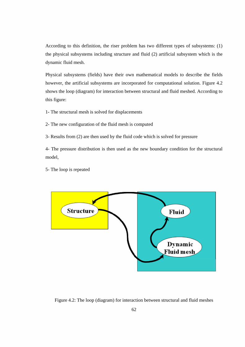
62

According to this definition, the riser problem has two different types of subsystems: (1)

the physical subsystems including structure and fluid (2) artificial subsystem which is the

dynamic fluid mesh.

Physical subsystems (fields) have their own mathematical models to describe the fields

however, the artificial subsystems are incorporated for computational solution. Figure 4.2

shows the loop (diagram) for interaction between structural and fluid meshed. According to

this figure:

1- The structural mesh is solved for displacements

2- The new configuration of the fluid mesh is computed

3- Results from (2) are then used by the fluid code which is solved for pressure

4- The pressure distribution is then used as the new boundary condition for the structural

model,

5- The loop is repeated

Figure 4.2: The loop (diagram) for interaction between structural and fluid meshes

63

4.3 Dynamic fluid mesh (ALE)

Generally, the fluid field is modeled using Eulerian method, by taking a fixed mesh over

the field. However, the treatment of moving boundaries and interfaces is difficult with

Eulerian elements. On the other hand, Lagrangian method is inapplicable to model fluid

field but is most common for the structural analysis. Therefore, some hybrid techniques

which combine the advantages of Eulerian and Lagrangian methods have been developed.

These methods which are called arbitrary Eulerian-Lagrangian formulation provide a

natural solution to this coupled system problem. In this method Eulerian formulation is

used in some part of the fluid filed and Lagrangian formulation is used for the structure

part. Then, ALE formulation is used for some deformable part as the fluid mesh around the

interface.

ALE accounts an arbitrary combination of the Lagrangian and Eulerian techniques that is

specified by the user through the selection of a mesh updated (motion) method.

4.4 Mesh update using a modified elasticity equation

Using an efficient mesh movement technique is important to get adequate results in the

ALE when we deal with large deformation problems. Indeed, solving mesh movement

uncoupled from structure and fluid field solutions makes it possible to apply some new

approaches to avoid mesh distortions. For this purpose, in this work a modified elasticity

equation in which the mesh ‘flow’ is governed by the modified equations of the elasticity

without body force and prescribed traction is used [65]

m=ΔK U R% % (4.1)

Where, K% is modified stiffness matrix and R% represents the fluid boundary displacements.

64

Figure 4.3: The techniques that are used for each subsystem

When mesh movement takes place, Equation (4.1) is solved to determine the internal nodal

displacement of the mesh based on the given data. Figure 4.3 shows the techniques that are

used for each subsystem during fluid-structure interaction uncoupled solution. After mesh

motion, data is transferred from the original mesh to relocated mesh using an extrapolation

procedure.

During large displacement analysis of deep water riser structure, the riser is displaced

significantly by the current loading. Therefore, moving the riser to its new position results

distortions in the fluid mesh. But in CFD it is important that the quality of the mesh near

the riser surface (where the cells are small) remains high. In order to avoid this problem, we

therefore propose two different approaches to modify elasticity equation matrices values.

( )L N L+ + =ΔU K K U RM &&

m=ΔK U R% %

65

1 - Taking the element volume ( t tV+Δ ) into account with a function of 21

t tV+Δ for

calculating Κ% .

2 - Taking both t tV+Δ and t t+Δ (a distance between riser centre and element centre) into

account with a function of 1( )t t t tV r+Δ +Δ %

for calculating Κ% .

Figure 4.4 shows a mesh of the fluid flow around a section of the riser structure. In Figure

4.5 this mesh updates after 0.1 m movement in horizontal direction using elasticity equation

for mesh modification. According to this result the small cells near riser boundary are

distorted. It is interesting to compare this result with those obtained by the modified

elasticity equation where the proposed modification approaches are considered.

Figure 4.4: Unmoved fluid mesh

66

Figure 4.5: Moved fluid mesh

In this approach, the elasticity equation is modified by taking the element volume into

account for calculating stiffness matrix. Figure 4.6 compares the results. In this figure red

cells show the moved mesh position with no modification in elasticity equation and black

cells show the moved mesh position calculated using modified equation. According to this

figure less distortion occurs at the small cells (black cells) when the modified elasticity

equation is used. Also, in the black mesh, most of displacements occur in elements far from

the riser center where the cells have larger volumes.

67

(a)

(b)

Figure 4.6: Compares the results, (a) red cells: moved mesh with no modification, black

cells: moved mesh with modification. (b) Zoomed on small cells

68

In this section, two different proposed modifications approaches for calculating elasticity

matrices during mesh movement are compared. For this purpose, the mesh shown in Figure

4.7 is considered. In Figure 4.8 a view of the initial mesh and the moved mesh is shown. In

order to obtain a better view for comparison of the results from the two different methods a

zoomed view is shown in Figure 4.9. In this figure blue lines show the moved mesh

position for the case that modification takes place using the function of 21

t tV+Δ for

calculating elasticity matrices and the black lines show the moved mesh position for the

case that the function of 1( )t t t tV r+Δ +Δ %

is used for modification.

Figure 4.7: A fine mesh case

69

Figure 4.8: A view of the initial mesh and the moved mesh

Figure 4.9: Compare the results from two different modification methods. Modification

takes place using functions 21

t tV+Δ (Blue lines) and 1( )t t t tV r+Δ +Δ %

(Black lines)

70

According to the Figure 4.9, for small cells near the riser surface there is no differences

between two results. But it seems that when using function 1( )t t t tV r+Δ +Δ %

for

modification, the majority of the distortions is transferred far from riser center where

normally use larger cells are used.

4.5 Non- matching meshes

In flexible riser fluid-structure interaction problem, the separate meshes that are used in the

fluid and structure domains do not matched at their common interface. In this problem, for

fluid we need a very fine mesh (Figure 4.10) specially around the riser surface to model

turbulent fluid flow. However, for long length riser structure a long coarse mesh can be

implemented to avoid high computational efforts.

Fluid

Structure

(a) (b)

Figure 4.10: (a) Very fine fluid domain mesh, (b) High course riser mesh

71

4.6 Transfer data between fluid and structure non- matched meshes

At the fluid-structure interface where the two meshes are potentially non-matched, the

important data has to be transfered between these incompatible meshes. Exchange of

information over this interface is therefore no longer trivial. There are several methods to

perform this data transformation. De Boer et al [66] have outlined six different methods.

The most common method for formulation of fluid-structure interaction problems is based

on using localized Lagrange multipliers [66]. In this method we introduce an interface

frame between the fluid and the structure at the interaction surface (Figure 4.11). Then

Local Lagrange Multipliers (LLM) links the sub-domains to the interface frame. The LLM

method requires that the partitioned boundary displacements be the same as the interface

frame displacements [64].

Figure 4.11: Introducing an interface frame between the fluid and structure interaction

surface

72

4.7 Analysis of a riser system subjected to current loading

Using the element described in this work a simple case study is carried out by subjecting

the nonlinear riser element to steady state flow loading (Figure 4.12). Here we are

considering a simple 2D steady state flow whose governing equations are:

Conservation of Mass: 0i

i

ux∂

=∂

(4.2)

Conservation of Momentum: 0ji ij ij i

j j j i

uu uu P fx x x x

ρ δ μ ρ∞ ∞

⎛ ⎞⎛ ⎞∂∂ ∂∂− − + + + =⎜ ⎟⎜ ⎟⎜ ⎟⎜ ⎟∂ ∂ ∂ ∂⎝ ⎠⎝ ⎠

(4.3)

Using the dimensionless variables * uuU∞

= , *2

ppUρ∞ ∞

= and Re U Dρμ

∞ ∞= as well as using

Galerkin least square method by preparing the weak forms of governing equations, the

mixed model of finite element formulation results in

11 22 21 1 1 1

12 11 22 2 2 2T T1 2

2K +K +C(u) K -Q u FK K +2K +C(u) -Q u = F-Q -Q 0 P 0

⎡ ⎤ ⎧ ⎫ ⎧ ⎫⎪ ⎪ ⎪ ⎪⎢ ⎥⎨ ⎬ ⎨ ⎬⎢ ⎥⎪ ⎪ ⎪ ⎪⎢ ⎥⎣ ⎦ ⎩ ⎭ ⎩ ⎭

(4.4)

where

ijK xe i j

dx x

μΩ

∂ ∂=

∂ ∂∫TN N iQ x

e i

dx

μΩ

∂=

∂∫ TN N 0C(u) ( ) xe

jj

u dx

ρΩ

∂=

∂∫T

T NN N (4.5)

where N is shape function vector of element used. A square 4-node element is used for

solution of the steady flow over the pipe section.

73

U=1.2 m/s

U=0.4 m/s

Figure 4.12: A pipe system subjected to steady state flow loading

In order to find the current loading on pipe structure the pressure coefficient ( pC )

distribution has been found at four levels (Figures 4.13), and for other parts of pipe

structure, a linear interpolation scheme has been used. The fluid mesh has been updated for

each increment, and on starting new increment the fluid domain was re-meshed with

reference to the new position of the riser and the data are interpolated from the last status.

The nonlinear response of this typical pipe due to calculated current loading is illustrated in

Figure 4.14.

74

-0.557-0.474-0.390-0.371-0.307-0.239-0.224-0.163-0.140-0.104-0.058 0.025 0.104 0.108 0.132 0.170 0.191 0.274 0.542 0.590 0.654

Cp distribution (Re= 134.83)

a: at top of pipe

-0.557-0.474-0.390-0.371-0.307-0.239-0.224-0.163-0.140-0.104-0.058 0.025 0.104 0.108 0.132 0.170 0.191 0.274 0.542 0.590 0.654

Cp distribution (Re= 104.83)

b: in depth 1.5 m

-0.557-0.474-0.390-0.371-0.307-0.239-0.224-0.163-0.140-0.104-0.058 0.025 0.104 0.108 0.132 0.170 0.191 0.274 0.542 0.590 0.654

Cp distribution (Re= 75.3)

c: in depth 3.0 m

-0.557-0.474-0.390-0.371-0.307-0.239-0.224-0.163-0.140-0.104-0.058 0.025 0.104 0.108 0.132 0.170 0.191 0.274 0.542 0.590 0.654

Cp distribution (Re= 45.)

d: at bottom of pipe

Figure 4.13: The pressure coefficient ( pC ) distribution at different levels

75

Displacement (m)

0

0.5

1

1.5

2

2.5

3

3.5

4

4.5U=4.5 m/s

U=0.4 m/s

A typicalnonlinear pipe response

0 1 2 3

Figure 4.14: The nonlinear response of typical pipe subjected to current loading

m

76

Chapter 5

Development of a Generalized Nonlinear Finite

Element Formulation to Analysis Unbounded

Multilayer Flexible Riser Using a Constitutive

Model

5.1 Introduction

A common approach for numerical analysis of riser structures is to use an equivalent

modeling scheme to simulate the existence of various layers which make up the structure of

a flexible riser. This approach fails to account for the interaction between layers, the

hysteresis effects due to occurrence of inter-layer slip-stick and also the nonlinear behaviors

due to friction between the unbounded layers.

Recently Bahtui et. Al. [6] presented a constitutive model for flexible riser structures. They

developed this constitutive model using the response of a limited length riser to bending

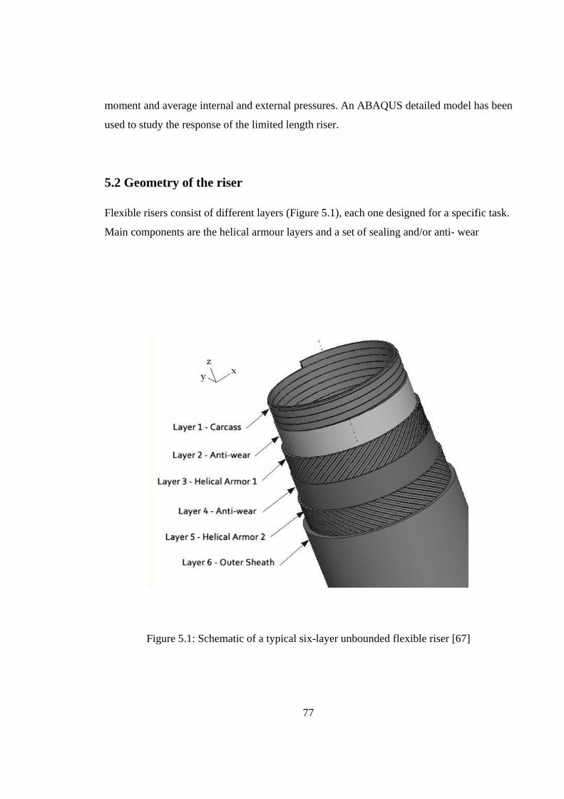
77

moment and average internal and external pressures. An ABAQUS detailed model has been

used to study the response of the limited length riser.

5.2 Geometry of the riser

Flexible risers consist of different layers (Figure 5.1), each one designed for a specific task.

Main components are the helical armour layers and a set of sealing and/or anti- wear

Figure 5.1: Schematic of a typical six-layer unbounded flexible riser [67]

78

polymer layers, while additional components which are typically present include a metallic

internal ‘carcass’ and a pressure armour layer. The geometry of an actual flexible pipe was

chosen from manufacturer as shown in Table 5.1.

Table 5.1: Flexible pipe geometrical data [67].

Layer Type ri (mm) ro (mm) r (mm) t (mm) α (degrees)

1 Carcass 85.54 90.54 88.04 5 88.44

2 Anti-wear Layer 90.76 97.46 94.11 6.7 90

3 Helical Armour 1 99.43 103.42 101.43 3.99 36.54

4 Anti-wear Layer 103.55 104.95 104.25 1.4 90

5 Helical Armour 2 105.17 109.17 107.17 4 -35.59

6 Outer Sheath 109.4 116.3 112.85 6.9 90

Definitions:

Type - Layer description

ri/ ro - Radius to layer inner/ outer surface

r - Layer mean radius

t - Layer thickness

79

All layers except the carcass layer were assumed to have isotropic type of properties. The

material data for the riser analysis is listed in Table 5.2. Modelling a three-dimensional

carcass layer in very detail leads to excessive computational solution time. The carcass

layer is thus replaced by an equivalent material and geometrically orthotropic layer.

The material property of the equivalent orthotropic layer was derived by comparing results

from the actual carcass layer and results from the embedded orthotropic sheath layer. The

orthotropic material properties are then evaluated using structural stability relations.

Table 5.2: Material data for the riser [67].

Layer Type E (N/mm2) ν yσ (N/mm2) ρ (kg/m3)

1 Carcass E1 = 1.50E+5

E2 = 1.24E+4 0.3 250 7860

2 Anti-wear Layer 3.50E+2 0.4 21 1030

3 Helical Armour 1 2.10E+5 0.3 740 7860

4 Anti-wear Layer 3.50E+2 0.4 21 1030

5 Helical Armour 2 2.10E+5 0.3 740 7860

6 Outer Sheath 3.50E+2 0.4 21 1030

80

A detailed three-dimensional finite element model is then developed under a global

cylindrical coordinate system with its origin located at the centre of riser bottom end.

Layers were modeled individually and then assembled together [67, 68]. Three-dimensional

contact interaction is also introduced between all layers, so that the layers are allowed to

slide with respect to each other during all stages of loading. The load cases considered are

tension, torsion, and bending. The analysis then is carried out as a geometrically non-linear

problem. This nonlinearity occurs due to the presence of contact surfaces as well as large

rigid body displacement taking place in the tendons of the helical armour layer. Abaqus

results show the hysteresis effect in the unbounded type of flexible riser which exists in all

load cases, but are particularly significant in the bending case, as shown in Figure 5.2,

where the loading and unloading paths are well distinct.

The results from various solutions are subsequently used to develop a constitutive model

for multilayer flexible riser structures.

 

Figure 5.2: Bending moment vs. curvature [67]

-10000

-5000

0

5000

10000

-0.03 -0.02 -0.01 0 0.01 0.02 0.03

Curvature (1/m)

Ben

ding

Mom

ent (

N.m

)

AbaqusAnalytical

O

AB

C

81

5.3 Constitutive model for multilayer flexible riser

Using the finite element details model results, Bahtui et. al. [6] proposed a model which

gives a relationship between generalized stress and strain components as follow

⎥⎥⎥⎥⎥⎥

⎦

⎤

⎢⎢⎢⎢⎢⎢

⎣

⎡

⎥⎥⎥⎥⎥⎥

⎦

⎤

⎢⎢⎢⎢⎢⎢

⎣

⎡

=

⎥⎥⎥⎥⎥⎥

⎦

⎤

⎢⎢⎢⎢⎢⎢

⎣

⎡

r

r

y

x

z

u

y

x

uDDDsym

DD

DDD

PP

MMN

ε

χχε

ε 55

5444

22

22

514111

.00000

00

(5.1)

In this model uyxt PMMMN ,,,, and εP are the generalized stresses. The corresponding

work-conjugated generalized strains are rryxz u εχχφε ,,,,, , where yxz χχε ,, and φ are the

axial strain, the curvatures about the x and y directions and the torsional curvature. The

detailed definition of the model is given in [6]. A compact notation is conveniently

introduced denoting by σ and ε the generalized stresses and strains:

⎥⎥⎥⎥⎥⎥⎥⎥

⎦

⎤

⎢⎢⎢⎢⎢⎢⎢⎢

⎣

⎡

=

⎥⎥⎥⎥⎥⎥⎥⎥

⎦

⎤

⎢⎢⎢⎢⎢⎢⎢⎢

⎣

⎡

=

r

r

y

x

z

u

y

x

t

uPP

MMMN

ε

χχφε

εσ

ε

(5.2)

Also components Dij values are given in [6]. In order to use this model, we then need to

develop a generalized nonlinear finite element formulation.

5.4 Generalized nonlinear finite element formulation

82

Next a generalized nonlinear finite element formulation is developed based on Euler-

Bernoulli beams theory with two extra degree of freedoms in riser radial and thickness

directions to fulfil all the required flexible riser degrees of freedom [6]. This finite element

formulation is also suitable to take the transitional constitutive model into the account for

analysing flexible riser structures. Referring to Figure 5.3, displacement components iu , iv

and iw for node i are defined as

0 00

( ) ( )( ) i ii i

w x u xu u x z yx x

∂ ∂= − +

∂ ∂ (5.3)

0 ( )i iv v x= (5.4)

0 ( )i iw w x= (5.5)

Figure 5.3: Euler-Bernoulli Beam Element with one extra degree of freedom to model riser

radial displacement

83

where i=1,2 indicates the node numbers, 0 ( )iu x , 0 ( )iv x and 0 ( )iw x are the displacement of

the centre-line in x, y and z directions, respectively. Also 0 ( ) /iw x x∂ ∂ and 0 ( ) /iu x x∂ ∂ are

rotation component about y and z axis for node i. Using relations (5.3)-(5.5) the nonlinear

strain–displacement relations, based on the von Karman’s assumption, are

2 2 2

0 0 0 0 02 2

12xx

u w v w vz yx x x x x

ε ∂ ∂ ∂ ∂ ∂⎛ ⎞= + + − +⎜ ⎟∂ ∂ ∂ ∂ ∂⎝ ⎠ (5.6)

0yyε = (5.7)

0xyε = (5.8)

Also, referring to the cross-sectional view of the riser in Figure 5.4, the average radial

strain rε is given by

in

inr t

tt −−=ε (5.9)

where tin and t denote the initial and the current thickness of the whole riser, respectively.

The radial displacement of the average radius, the radial displacement of the internal layer

and the radial displacement of the external layer, indicated with int,uur and extu ,

respectively, are related to the radial strain and to the current thickness as follows:

2

2int

tuu

tuu

rrext

rr

ε

ε

−=

+=

(5.10)

84

Figure 5.4: Cross view of the riser section [6]

To develop a nonlinear finite element model for this Euler-Bernoulli beam element we

interpolate the displacement values as well as generalized strain components ru and rε in

the element field using their nodal values as follows

1 1 2 2u N u N u= + (5.11)

3 1 4 2 5 1 6 2v N v N v N Nθ θ= + + + (5.12)

3 1 4 2 5 1 6 2w N w N w N Nθ θ= + + + (5.13)

1 1 2 2r r ru N u N u= + (5.14)

1 1 2 2r r rN Nε ε ε= + (5.15)

0

0

ttt

r−

=ε

ru

int  

t  

intR  

extR  

85

where u1 and u2 are the axial nodal displacements, w1 and w2 are transitional displacements,

1θ and 2θ are nodal rotational components. Also in Equations (5.11)-(5.15), N1 and N2 are

linear shape functions however N3-N6 are cubic shape function (Figure 5.5).

Here to develop governing nonlinear finite element formulation for Euler-Bernoulli beam

we need to define bending curvature components, as follows

2

2

3/ 22

1x

wxwx

χ

∂∂=

⎡ ⎤∂⎛ ⎞+⎢ ⎥⎜ ⎟∂⎝ ⎠⎢ ⎥⎣ ⎦

(5.16)

Figure 5.5: Cubic shape function

86

For this nonlinear problem, the governing equation in rectangular Cartesian coordinates is

derived using the principle of minimum total potential energy, i.e.

( )

( )

* *

* *

b

a

xei extg gx

NLg

g g

W dx

f

σ ε

ε

σ ε

= • = •

= Β

=

∫ F q

q

%

% (5.17)

where σ and ε are given in (5.2).Using (5.17) the incremental finite element equation of

equilibrium can be written as:

( ) ( ) 0int ext= − =R q F q F (5.18)

where ( )1 1 1 1 2 2 2 2T

r ru w u u w uθ θ=q . Implementing Newton-Raphson method to solve

the Equation (18) leads to

( )1 1( ) ( )1 1 11 1

k kn n

k k nn n tNL ext int+ +

+ − ++ += + −q qq q k F F (5.19)

where

1

1( ) detk

NL n

kn

TtNL NL NLV

d dVd ε

σε

+

+

== ∫

B qqk B B J

)

)

) (5.20)

87

where

1

1 1 1 1 1

21 12 5 1 2 16 172

13 5 4 6

1 2

( )

2 2 20 0

0 / / 0 0 / / 0

0 0 0 0 0 02 2

k

n

k k k k k

n n n n n

ktNL

N k N N k kl l l

N N N Nl lN N

θ

τ τ τ τ

+

+ + + + +

+

⎡ ⎤′ ′ ′⎢ ⎥⎢ ⎥′′ ′′ ′′ ′′= ⎢ ⎥⎢ ⎥

′ ′⎢ ⎥⎣ ⎦

qB

(5.21)

1 1 1 1

312 3 1 4 2 5 1 6 22

2 ( 2 2 )k k k k

n n n n

Nk N w N w N Nl

θ θ+ + + +

′′ ′ ′ ′= + + + (5.22)

1 1 1

416 4 2 5 1 6 22

2 ( 2 2 )k k k

n n n

Nk N w N Nl

θ θ+ + +

′′ ′ ′= + + (5.23)

1 1

617 6 2 5 12

2 ( 2 )k k

n n

Nk N Nl

θ θ+ +

′′ ′= + (5.24)

( )( )1 1 1 1 1

3/ 22

3 1 4 2 5 1 6 21k k k k k

n n n n nN w N w N Nτ θ θ

+ + + + +′ ′ ′ ′= + + + + (5.25)

The derivation of the consistent tangent operator 1

kNL n

dd ε

σε

+=B q)

)

) is given in [6].

88

5.5 Application to a cantilever riser subjected to an end bending moment

Consider a cantilever flexible riser with length 500 m which is subjected to an end bending

moment (1500 N.m). Figure 5.6 depicts the result for this flexible riser for three different

condition: Linear solution with constant EI=608108, nonlinear solution with constant

EI=608108 and nonlinear solution with the inclusion of the constitutive model with initial

value EI=608108 (the first EI value which is taken from the constitutive model’s output).

From Figure 5.6 it is noted that the presented constitutive model [6] is capable of capturing

the energy dissipation in flexible riser structure due to frictional slip between layers and the

hysteretic response. According to [67], finite element analysis of a details model of a

flexible riser using finite element software on a cluster of parallel processors took many

hours to arrive at the solution. Using the developed constitutive model and a generalized

finite element formulation, however, we are able to study the nonlinear behavior of a long

length of flexible risers by getting the results in seconds. This example shows the capability

and importance of the proposed constitutive model

89

Displacement (m)

Leng

th(m

)

0 100 200 300 400 500-50

0

50

100

150

200

250

300

350

400

450

500

550

Initial PositionLinear Solution with EI=608108 (Constant)Nonlinear Solution with EI=608108 (Constant)Nonlinear solution using constitutive model to calculate EI

Bending MomentM=1500 N.m

Figure 5.6: Cantilever riser subjected to an end bending moment

90

Chapter 6

Results Verification

6.1 Introduction

Based on the presented finite element formulation in previous chapters a finite element code

has been developed. Using this code we study linear and nonlinear behavior of the riser

structures subjected to various loading conditions. The results are verified by making

comparisons to those available in the literature.

6.2 Curve pipe under end loading

A curved pipe structure subjected to a concentrated end load, F, as shown in Figure 6.1 is

considered in this example. Mechanical properties and geometrical dimensions of this

structure are shown in the figure. Figure 6.2 shows the results from linear solution of the

structures those obtained from the proposed 3D annular section beam element and also

from a 2D beam element of ABAQUS [69], where a good agreement is achieved.

 

91

 

 

 

 

Elemen

No. 2

Elemen No. 1

Elem

enN

o.3

R=3.07 m

t=5 mm

Corss section:

a=10 Cm

4

Node 1

32

5

6

7

8

9

10

Material:

E=207E9 PaNu=0.3

Figure 6.1: A curved pipe structure nodes, elements, geometry and material properties

92

Initial configurationDeformed shape, this workDeformed shape, ABACUS

F

Figure 6.2: Configuration, initial and deformed

ABAQUS

93

6.3 Large deformation analysis results

A cantilever pipe subjected to an end load with length 4.5 m is analyzed in this example.

Results are depicted for load versus deflection in Figure 6.3. This figure shows the

difference between linear and nonlinear solutions. In addition, the history of displacement

during the incremental solution of the same cantilever pipe structure is shown in Figure 6.4.

According to the results, there is a considerable difference between the results from the

linear and nonlinear solutions in large deformation region. Also, it is noted that the

proposed Algorithm gives convergence for nonlinear solution with less solution effort [15].

6.4 A cantilever beam loaded by a uniformly distributed

displacement-dependent normal pressure

A cantilever beam which is loaded by a uniformly distributed displacement-dependent

normal pressure lP along its length (Figure 6.5) is considered. Therefore, as the beam

deforms the load remains normal to the beam’s centre-line. Figure 6.6 shows the horizontal

and vertical displacements as well as the rotation at the central point of the free end versus

non-dimensional load parameter 3 /( )lP l EIβ = . Bathe et al. [70] used a standard

linearization method which gave a limited range of deflections in vertical direction for low

values of the load parameter β . Also, Argyris and Symeonidis [71] could not control the

flutter problem after 28β = when using their natural mode based theory. Using the

presented finite element formulation with just three elements, we have managed to solve

the same problem for up to 52.6β = . The history of the deformation of the beam is also

shown in Figure 6.7.

94

Load ( time step)

Dis

plac

emen

t(tip

)(m

)

0

0.5

1

1.5

2

2.5

3

3.5

4

4.5

NonlinearLinear

10.750.50.250

a(outer radius) = 0.1 mt(thickness)= 0.1428571429e-2 m

Fy= 150000 N

Length= 4.5 m

Figure 6.3: Comparing the linear and nonlinear solution

95

Length (m)0 1 2 3 4

0

0.5

1

1.5

2

2.5

3

3.5

4Length=4.5 m

Fy=150000 N

a(outer radius) =0.1 mt(thickness)=0.1428571429e-2 m

History of Displacement

Figure 6.4: History of displacement during incremental solution

96

Figure 6.5: Cantilever beam loaded by a uniformly distributed follower normal pressure lP

97

X

X

X

X

X

X

-u1 /l, -u3 /l, 2 /l

β

-0.5 0 0.5 1 1.5 2 2.5 3 3.50

10

20

30

40

50

Present workPresent workPresent workArgyris and Symeonidis [17]Argyris and Symeonidis [17]Argyris and Symeonidis [17]Bathe et al. [16]

X

θ2 /

-u1 /l

- u3 /l l

β = PLl3/EI

θ

Figure 6.6: Large displacement and rotation at the free end of the cantilever beam

98

-2 -1 0 1 2 3 4 5

-1

0

1

2

3

4

5

Initial configuration of the Beam

β=52.6

β=0.0

Figure 6.7: Deformed geometry of the beam mid-line

99

6.5 Flexible cantilever riser structure subjected to buoyancy force

Consider a flexible cantilever polyethylene riser structure with internal diameter 0.8m ,

external diameter 0.85m and length 20.0m . This structure is capped at both ends and is

placed at 100.0m below the water surface. The riser is loaded with a vertical point load

with value 510 kN at the free end. The unit weight of the pipe and sea water are 312000 /wp N mρ = and 310250 /ww N mρ = , respectively. Also, the pipe material properties

used are: modulus of elasticity, 2.0GPa and Poisson’s ratio 0.25. In the present work, the

riser cross section is homogeneous and the slippage between layers is ignored.

Yazdchi and Crisfield [17] used a two dimensional model to analyze this problem. The

purpose of the analysis is to find the final configuration of the beam under gravity

combined with external and buoyancy loads. Figure 6.8 depicts the deformed configuration

with and without consideration of buoyancy force. In this figure, the result from the

presented formulation is compared with those given by [17]. As can be seen the two sets of

predictions provide very close comparisons. Moreover, it is also observed that the

maximum displacement values obtained from the present formulation are lower than those

reported in literature. These differences may arise due the accuracy which is implied in the

present finite element formulation during the linearization process. Also, from these results

it is noted that buoyancy force has a significant effect on flexible riser behaviors. Figure 6.9

shows axial stress distribution at outer surface in the root of cantilever riser through the

circumferential direction. According to this figure, the maximum axial stress value

increases up to %65 when the buoyancy force has been considered. Figures 6.10 also

illustrate the axial stress distribution contour in a cross section at the root of cantilever riser.

From these results it is noted that buoyancy force has a significant effect on flexible riser

behaviors. Also figures 6.9 and 6.10 demonstrate the capabilities of the present formulated

element which gives the stress distribution around the pipe circumferences at each

particular point in the riser.

100

x x x x x x x x x x x x xx

xx

xx

xx

xx

x x x x x x xx

xx

xx

xx

xx

xx

xx

xx

x x x x x x x x x x x x x x x x x x x x x x

x x x x x x x x x x x x x x x x x x x x x x

Length (m)

y(m

)

0 2 4 6 8 10 12 14 16 18 20-12

-10

-8

-6

-4

-2

0

2

4

6

8

10

12Yazdchi & Crisfield 2002This work

x

Up-ward loading with buoyancy

Down-ward loading

Down-ward loading with buoyancy

Up-ward loading

Figure 6.8: Deformed configuration of the flexible cantilever polyethylene pipe with and

without considering buoyancy force

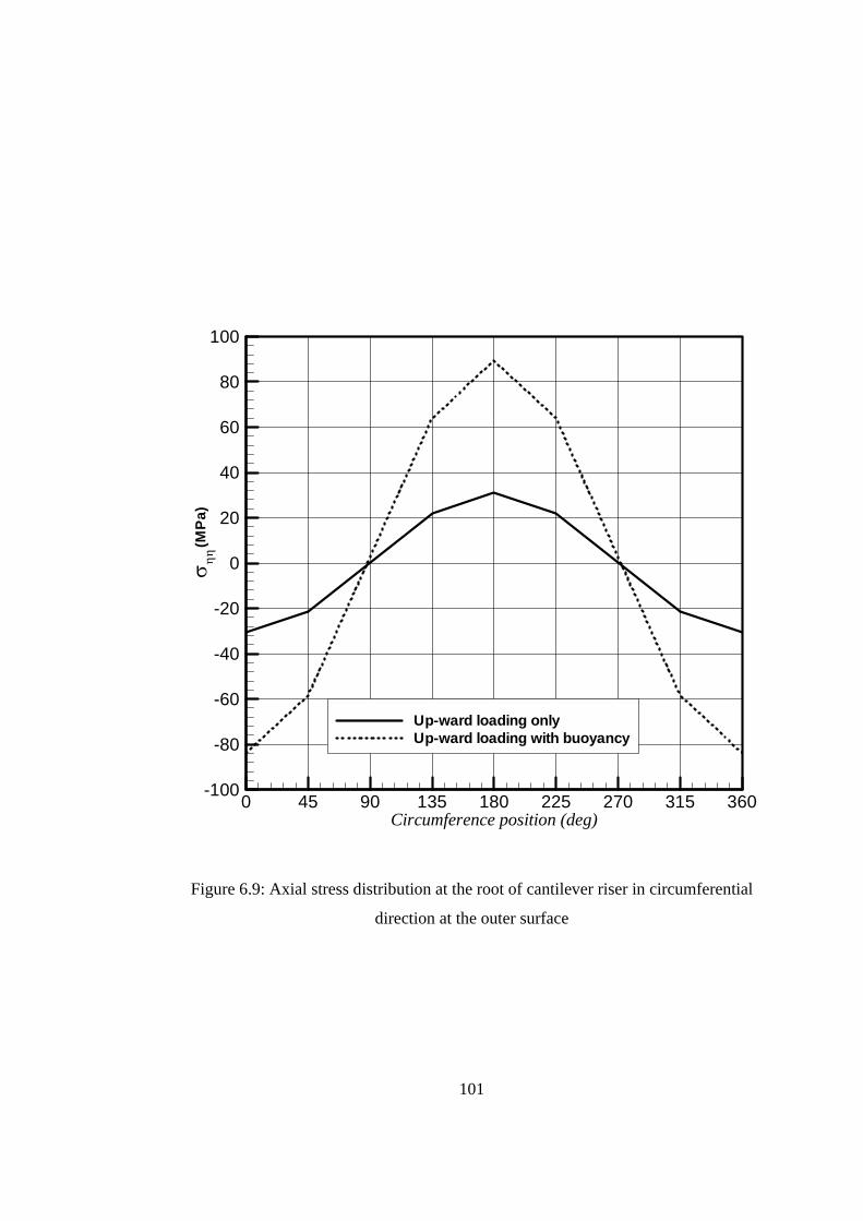
101

Circumference position (deg)

σ ηη

0 45 90 135 180 225 270 315 360-100

-80

-60

-40

-20

0

20

40

60

80

100

Up-ward loading onlyUp-ward loading with buoyancy

(MP

a)

Figure 6.9: Axial stress distribution at the root of cantilever riser in circumferential

direction at the outer surface

102

s1(MPa): -70.42-57.12-43.81-30.50-17.19 -3.88 9.43 22.74 36.05 49.36 62.67 75.97

(a)

s1(MPa): -26.20-21.79-17.37-12.96 -8.55 -4.13 0.28 4.69 9.11 13.52 17.93 22.34 26.76

(b)

Figure 6.10: Axial stress distribution contour in a cross section at the root of cantilever riser

(a) Up-ward loading only (b) Up-ward loading with buoyancy force

103

6.6 A vertical riser subjected to a riser top-tension and current loading

A 320.0 m length riser (Figure 6.11) with internal and external diameters 0.21 m and 0.25 m

is considered. In this example the behavior of a riser top-tension, which is attached to a

floating system, with top tension force 510.0 kN is evaluated. A modulus of elasticity 2.0 ×

1011 N/m2 and a Poisson’s ratio of 0.25 is used for this riser. The water depth is taken as

300.0 m and the unit weight of pipe and sea water are 77000.0 N/m3 and 10250.0 N/m3,

respectively. Also, for steady state current, the transverse and tangential drag coefficients

are 1.0 and 0.01, respectively.

The riser is modeled with thirty elements equally spaced below the water level and four

elements equally spaced above it. It is assumed that the riser is initially vertical with the

bottom node being hinged and the top-tension force being applied to the top point

vertically. Figure 6.12 presents the deformed configuration for two different magnitudes for

the uniform current profile, namely 1.0 and 2.0m/s. Yazdchi and Crisfield [17] have used a

two-dimensional finite element analysis of flexible risers to solve this problem. As can be

observed in Figure 6.12, a very good agreement is obtained between the results in

moderately large displacement region but in the very large displacement region, the two

sets of results diverge due to the accuracy which is implied in the present finite element

formulation during the linearization process.

104

Figure 6.11: a vertical riser which is attached to the floating system (top tensioned)

105

xx

xx

xxxxxxxxxxxxxxxxx

xx

xx

xx

xx

xxx

xxx

xx

xx

xx

xx

xx

xxxxxx

xx

xx

xx

xx

xx

xx

xx

xxxxx

Displacement (m)

Leng

th(m

)

0 3 6 9 12 15 18 21 24 27 300

25

50

75

100

125

150

175

200

225

250

275

300

325

350

Yazdchi & Crisfield 2002This work

x

Cur

rent

velo

city

=1.

0m

/s

Cur

rent

velo

city

=2.

0m

/s

Figure 6.12: Deformed configuration of riser considering two different magnitudes for the

uniform current profile, namely 1.0 and 2.0m/s

106

6.7 Riser subjected seabed boundary condition

In order to study the effects of using pipe-soil interaction model to identify seabed

boundary condition on flexible riser behavior, in this example the same polyethylene pipe

example 4 is considered to be laid down at the seabed. The calculated initial penetration

depth for this riser on the seabed with a given material properties is 0.28 m (Figure 6.13).

For this example an onsoy clay seabed with undrained shear strength 350 10uS kPa= × ,

310CF N= and 20.7 /Vc m year= is considered. Also the pull-out velocity assumes

0.05 /pV m s= . Figure 6.14 represents deformed configuration of the flexible cantilever

polyethylene pipe with and without the seabed boundary condition. From these results it is

concluded that including a suitable model for the pipe-soil interaction obtains a more

realistic and accurate results for deep water flexible riser structures.

6.8 Flexible riser subjected to a horizontally boundary movement

For this example a horizontal flexible riser structure with simply supported boundary

condition at both ends is considered. This riser has an initial length of L=142.5 m, first

configuration span l=130 m, cross sectional area A0=8×10-3 m2,moment of inertia

J0=5.1×10-6 m4 and modulus of elasticity E=100 GPa.

A static analysis is conducted to move the right end boundary of this riser structure

horizontally to the left by 105 m. Figure 6.15 shows the configurations of this riser

structure at three different stages of the boundary movement. Lacarbonara and Pacitti [54]

solved this problem using an exact analytical formulation with flexural stiffness effects. It

can be seen in this figure that the results from the presented finite element formulation are

in very good agreement with those from the exact analytical solution [54].

107

 

 

 

Figure 6.13: The calculated initial penetration depth (0.28 m)

 

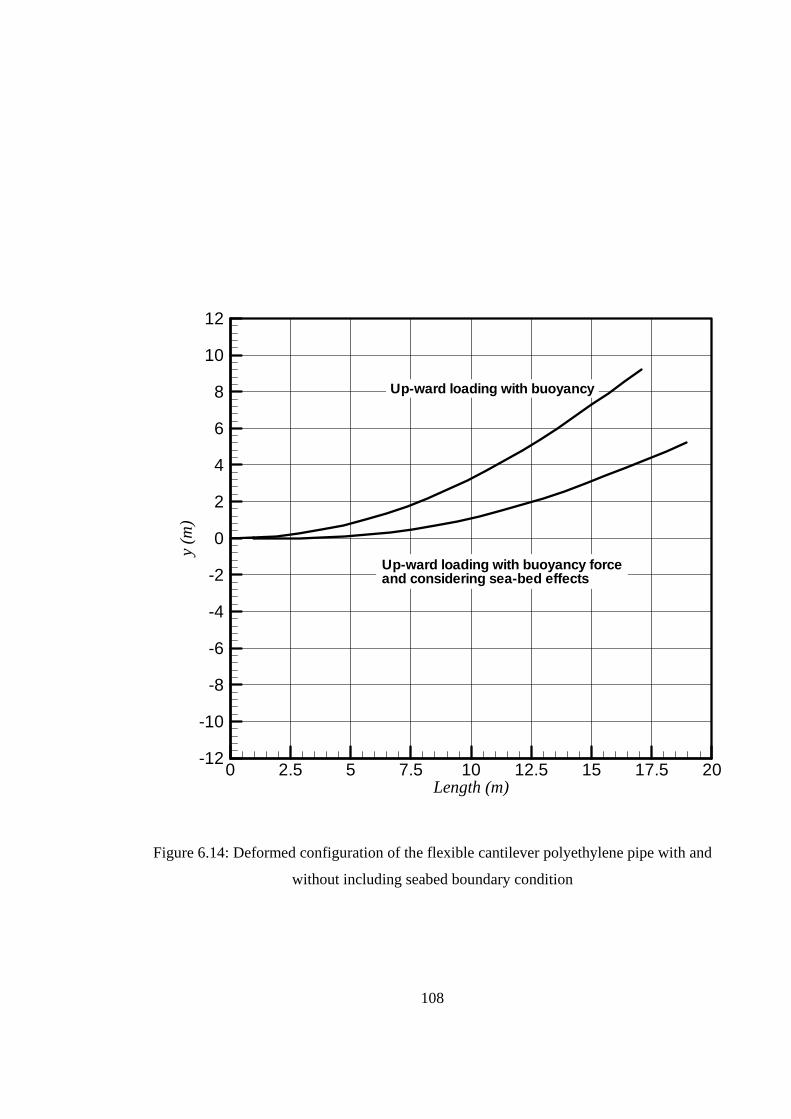
108

Length (m)

y(m

)

0 2.5 5 7.5 10 12.5 15 17.5 20-12

-10

-8

-6

-4

-2

0

2

4

6

8

10

12

Up-ward loading with buoyancy

Up-ward loading with buoyancy forceand considering sea-bed effects

Figure 6.14: Deformed configuration of the flexible cantilever polyethylene pipe with and

without including seabed boundary condition

109

Length (m)

Dis

plac

emen

t(m

)

0 10 20 30 40 50 60 70 80 90 100 110 120 130 140-90

-80

-70

-60

-50

-40

-30

-20

-10

0

10

Initial static configurationAfter boundary movement (35 m)After boundary movement (70 m)After boundary movement (100 m)Lacarbonara and Pacitti 2008

105 m (boundary movement)

Figure 6.15: Deformed configuration of horizontal flexible riser

110

6.9 Flexible riser subjected to a periodically ship movement

For this example a flexible riser system with external diameter 0.26 m, internal diameter 0.2

m and bending stiffness 20.96 x 103 N-m2 at 150 m water depth is analyzed (Figure 6.16).

The upper point is to be connected to a surface floating vessel which is displaced 150 m

horizontally and the other end is fixed to a sub-sea tower at a depth of 150 m. Both ends can

rotate freely. The riser length is 350 m. The riser is divided into twenty elements. Details of

element discretization can be found in reference [16]. It is assumed that the riser is filled

with seawater. Mass density of seawater is 1025 kg/m3 and mass per unit length of the riser

is considered to be 57.5 kg/m. This particular riser system has already been analyzed by

Yazdchi and Crisfield [16] using a 3D beam element. The transverse and tangential drag

coefficients are 1.0 and 0.0, respectively. The loading condition includes a steady state

current load together with buoyancy force effects.

A static analysis has initially been conducted to move the pipe from its horizontal

configuration at a depth of 150 m to its final shape as shown in Figure 6.16 using both force

and displacement controls, sequentially. The bending moment diagram of the flexible riser

in its final configuration is plotted in Figure 6.17 which is shown to be consistent with that

reported by Yazdchi and Crisfield [16]. Subsequently, the riser is analyzed dynamically for

forces due to ship movement with amplitude of 2.01 m and a corresponding period of 14.0

s. The results of this analysis for the sub-sea connected node are shown in Figure 6.18. As

ship movement imposes moderately large displacement to the flexible riser, there is a good

agreement between the results from present formulation and those presented in [16].

111

Figure 6.16:. Deep water flexible riser

112

Distance along the riser (m)

Ben

ding

Mom

ent(N

-m)

0 50 100 150 200 250 300 3500

100

200

300

400

500

600

700

Present workYazdchi & Crisfield 2002

Figure 6.17: Bending moment diagram

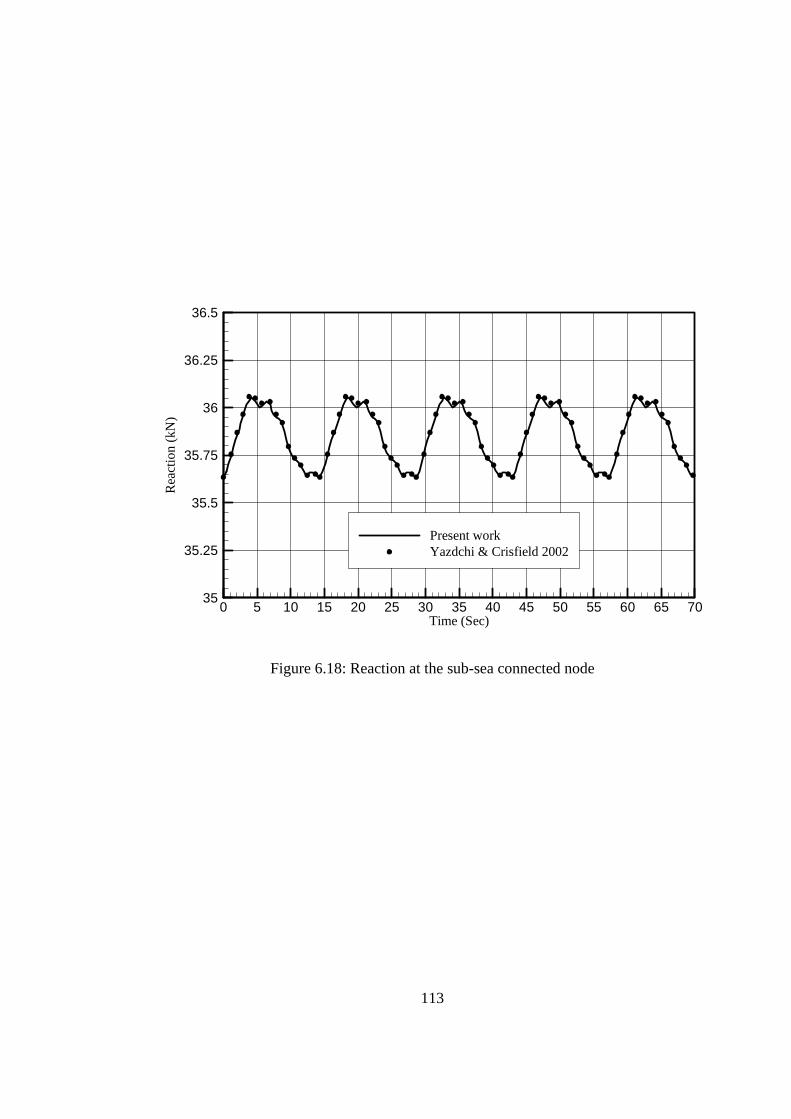
113

Time (Sec)

Rea

ctio

n(k

N)

0 5 10 15 20 25 30 35 40 45 50 55 60 65 7035

35.25

35.5

35.75

36

36.25

36.5

Present workYazdchi & Crisfield 2002

Figure 6.18: Reaction at the sub-sea connected node

114

Chapter 7

Conclusions and recommendations for future work

7.1 Conclusions

A finite element formulation was presented for geometrically nonlinear dynamic analysis of

flexible riser structures in presence of steady state current, riser-soil interaction and

buoyancy forces.

The formulation has been derived using an incremental updated Lagrangian approach

together with a modified linearization scheme for a three-dimensional flexible riser

element. Decomposing the Green-Lagrange strain and the 2nd Piola-Kirchhoff stress into

two second-order six termed functions of through-the-thickness parameters, made it

possible to explicitly account for the nonlinearities in the direction along the thickness.

Moreover, these decompositions led to a particular linearization scheme using Taylor series

expansion. It is noted that the employed efficient linearization scheme avoids inaccuracies

normally associated with other linearization methods.

115

The proposed nonlinear finite element formulation has been implemented in a finite

element code using a proper nonlinear algorithm. This code is then used to model and

analyze some typical riser configurations subjected to the various loading conditions.

Some examples of flexible riser were solved and the results have been compared with those

available in the literature. Concerning a flexible cantilever riser subjected by a follower

distributed pressure; it has been shown that displacements are in good agreements for

moderate range of displacements. According to the results the difference between the

results from the present formulation and those in the literature gradually increases when we

deal with larger displacements and rotations in flexible riser structures. It is considered that

the difference between the two sets of results diverges due to the accuracy which is implied

in the present finite element formulation because the linearization process.

The fluid-solid interaction problem is a significant concern in flexible riser structures

where there is a strong coupling between the fluid motion and the risers dynamics behavior.

Chapter 4 has therefore been devoted to developing an efficient riser problem fluid-solid

interaction algorithm. Two different approaches have been proposed to modify the fluid

mesh flow governing elasticity equation matrices. From the result it is noted that both two

approaches keep the smaller cells from distortions while the fluid mesh is moved in

accordance with the riser’s motion.

In view of the fact that the equivalent modeling scheme for simulation of the various layers

of a flexible riser fails to model multi layer flexible riser behavior properly, using a more

accurate constitutive model for flexible riser structures Using detailed finite element

simulation of the risers unbonded layers the constitutive model characterizes the behavior

of various riser’s layers subjected to different modes of loading. In Chapter 5 this

constitutive model is implemented into a generalized finite element formulation which has

been developed based on Euler-Bernoulli beam element formulation together with two new

degrees of freedom. From the result it is noted that using the constitutive model together

with the developed generalized finite element formulation, capability is developed to study

the nonlinear behavior of a long length of flexible risers in a very short time.

116

7.2 Recommendations for future work

The following suggestions are put forward for future investigations.

• Development of a flexible riser constitutive model for proposed nonlinear flexible

riser element

• Implementation of the proposed approaches for fluid mesh movement in a fluid

code and developing an ALE formulation for the riser problem

• Implementation of the developed flexible riser element together with constitutive

model in a fluid code to study VIV

117

Bibliography

1. O'Brien, P. J. and McNamara, J. F. (1988). ‘Analysis of flexible riser systems

subject to three-dimensional sea state loading’, Proceedings of the international

conference on behaviour of offshore structures, BOSS 88, Trondheim, Norway, 6

1373-1388.

2. Machado, Z.L. and Dumay, J.M. (1980). ‘Dynamic production riser on Enchova

field offshore Brazil’, Offshore Brazil conference, Latin America Oil Show, Rio de

Janeiro.

3. Out, J.M.M., Kronemeijer, D.A., van de Loo, P.J. and de Sterke, A. (1995). ‘The

integrity of flexible pipe: search for an inspection strategy’, Engineering structures,

17, 4 305-314.

4. Kraincanic, I. and Kebadze, E. (2001). ‘Slip initiation and progression in helical

armouring layers of unbonded flexible pipes and its effect on pipe bending

Behaviour’, Journal of Strain Analysis, 36, 3 265-275.

5. Kagoura, T., Ishii, K., Abe, S., Inoue, T., Hayashi, T., Sakamoto, T., Mochizuki, T.,

and Yamada, T. (2003). Development of a Flexible Pipe for Pipe-in-pipe

Technology, Furukawa Review 24: 69-75.

6. Bahtui A., Hosseini-Kordkheili S.A., Bahai H., Alfano G. (2008e). ‘A multi-scale

computational model for unbonded flexible risers’, Under development.

7. Hosseini Kordkheili S.A., Naghdabadi R. (2007), Geometrically Nonlinear

Thermoelastic Analysis of Functionally Graded Shells Using Finite Element

Method, International Journal for Numerical Methods in Engineering, 72, 964-986.

8. Arciniega R.A., Reddy J.N. (2007), Tensor-based finite element formulation for

geometrically nonlinear analysis of shell structures, Computer Methods in Applied

Mechanics and Engineering, 196, 1048–1073.

118

9. Arciniega R.A., Reddy J.N. (2007), Large deformation analysis of functionally

graded shells, International Journal of Solids and Structures, 44, 2036-2052.

10. Yu W., Hodges D.H.(2004), A geometrically nonlinear shear deformation theory for

composite shells, Journal of Applied Mechanics, 71, 1-9.

11. Woo J., Meguid S.A. (2001), Nonlinear analysis of functionally graded plates and

shallow shells, International Journal of Solids and Structures, 38, 7409-7421.

12. Yoo S.W., Choi C.K. (2000), Geometrically nonlinear analysis of laminated

composites by an improved degenerated shell element, Structural Engineering and

Mechanics, 9, 99-110.

13. A. Masud, C.L. Tham, W.K. Liu (2000), A stabilized 3-D corotational formulation

for geometrically nonlinear analysis of multi-layered composite shells,

Computational Mechanics, 26, 1–12.

14. C.L. Tham, Z. Zhang, A. Masud (2005), An elastoplastic damage model cast in a

corotational kinematic framework for large deformation analysis of laminated

composite shells, Computational Methods in Applied Mechanical Engineering, 194,

2641–2660.

15. Hosseini Kordkheili S.A., Bahai, H. (2008), Non-linear finite element analysis of

flexible risers in presence of buoyancy force and seabed interaction boundary

condition, Archive of Applied Mechanics, 78, 765-774.

16. Yazdchi M., Crisfield M.A. (2002), Nonlinear Dynamic Behaviour of flexible

marine pipes and risers, International Journal for Numerical Methods in

Engineering, 54, 1265–1308.

17. Yazdchi M., Crisfield M.A. (2002), Buoyancy forces and the 2D finite element

analysis of flexible offshore pipes and risers, International Journal for Numerical

Methods in Engineering, 54, 61–88.

119

18. Hosseini Kordkheili S.A., R. Naghdabadi and M. Jabbarzadeh (2008), A

Geometrically Nonlinear Finite Element Formulation for Shells Using a Particular

Linearization Method, Journal of Finite Element in Analysis and Design, 44, 123-130.

19. Zielinski A.P., Frey F. (2001), On linearization in non-linear structural finite

element analysis, Computers and Structures, 79, 825-838.

20. Bathe K.J. (1982), Finite element procedures in engineering analysis, Prentice Hall.

21. Bathe K.J., Ramm E., Wilson E.L. (1975), Finite element formulation for large

deformation dynamic analysis, International Journal of Numerical Methods in

Engineering, 9, 353-389.

22. Bathe K.J., Almeida C.A. (1980), A simple and effective pipe elbow element –

linear analysis, Journal of Applied Mechanics, 47, 93-100.

23. Bathe K.J., Almeida C.A., Ho L.W. (1983), A simple and effective pipe elbow

element, some nonlinear capabilities, Computers and Structures, 17, 659-667.

24. Massin P., Al Mikdad M. (2002), Nine node and seven node thick shell elements

with large displacements and rotations, Computers and Structures 80, 835–847.

25. Jiang L.C., Michael W., Pegg Neil G. (1994), Corotational updated Lagrangian

formulation for geometrically non-linear finite element analysis of shell structures,

Finite Element in Analysis and Design, 18, 129-140.

26. Lee S.J., Kanok-Nukulchai W. (1998), A nine-node assumed strain finite element

for large-deformation analysis of laminated shells, International Journal of

Numerical Methods in Engineering, 42, 777-798.

27. Moita G.F., Crisfield M.A. (1996), A finite element formulation for 3-D continua

using the corotational technique, International Journal of Numerical Methods in

Engineering, 39, 3775-3792.

120

28. Kanok-Nukulchai W., Taylor R., Hughes T.J.R. (1981), A large deformation

formulation for shell analysis by the finite element method, Computers and

Structures, 13, 19-27.

29. Crisfield M.A. (1981), A fast incremental/iterative solution procedure that handles

snap-through, Computers and Structures, 13, 55-62.

30. Peng X., Crisfield M.A. (1992), A consistent corotational formulation for shells

using the constant stress/constant moment triangle, International Journal of

Numerical Methods in Engineering, 35, 1829-1847.

31. Djoudi M.S., Bahai H. (2003), A shallow shell finite element for the linear and

nonlinear analysis of cylindrical shells, Engineering Structures, 25, 769-778.

32. Prema Kumar W.P., Palaninathan R. (1994), Explicit through-thickness integration

schemes for geometric nonlinear analysis of laminated composite shells, Finite

Element in Analysis and Design, 18, 129-140.

33. Brack, M., Troina, L.M.B. and Sousa, J.R.M. (2005). ‘Flexible riser resistance

combined axial compression, bending, and torsion in ultra-deep water depths’,

Proceedings of 24th International Conference on Offshore Mechanics and Arctic

Engineering, OMAE05, June 12-17, Halkidiki, Greece.

34. API Recommended Practice 17B. (2002). Recommended Practice for Flexible Pipe,

American Petroleum Institute.

35. API Specification 17J. (2002). Specification for Unbounded Flexible Pipe, 2nd Ed.

American Petroleum Institute.

36. Knapp, R.H. (1979). ‘Derivation of a new stiffness matrix for helically armoured

cables considering tension and torsion’, International Journal for Numerical

Methods in Engineering, 14, 4 515-529.

121

37. Felippa, C.A., Chung, J.S. (1980), Nonlinear Static Analysis of Deep-ocean Mining

Pipe EM DASH 1. Modeling and formulation, American Society of Mechanical

Engineers, 80, 48: 6pages.

38. Felippa, C.A., Chung, J.S. (1981), Nonlinear Static Analysis of Deep-ocean Mining

Pipe EM DASH 1. Modeling and formulation, Journal of Energy Resources

Technology, Transactions of the ASME, 103, 11-15.

39. McNamara, J.F., Lane, M. (1984), Practical Modelling for Articulated Risers and

Loading Columns, Journal of Energy Resources Technology, Transactions of the

ASME, 106, 444-450.

40. McNamara, J.F., Lane, M. (1992), 3D Frequency Domain Analysis of Offshore

Structures, Proceedings of the 9th Conference on Engineering Mechanics, College

Station, TX, USA, 192-195.

41. O'Brien, P.J., McNamara, J.F. and Dunne, F.P.E. (1988), Three-dimensional

Nonlinear Motions of Risers and Offshore Loading Towers, Journal of Offshore

Mechanics and Arctic Engineering, 110, 232-237.

42. McNamara, J. F., and O'Brien, P. J. and Gilroy, S. G. (1988). ‘Nonlinear analysis of

flexible risers using hybrid finite elements’, Journal of Offshore Mechanics and

Arctic Engineering, 110, 3 197-204.

43. Hoffman, D., Ismail, N., Nielsen, R. and Chandwani, R. (1991), Design of Flexible

Marine Riser in Deep and Shallow Water, Proceedings 23rd Annual Offshore

Technology Conference, OTC91, Houston, TX, USA, 253-265.

44. Atadan, A.S., Calisal, S.M., Modi, V.J., and Guo, Y. (1997), Analytical and

Numerical Analysis of the Dynamics of a Marine Riser Connected to a Floating

Platform, Ocean Engineering, 24, 111-131.

122

45. Chai Y.T., Varyani K.S., and Barlt N.D.P. (2002), Three-dimensional Lump-mass

Formulation of a Catenary Riser with Bending, Torsion and Irregular Seabed

Interaction Effect, Ocean Engineering, 29, 1503–1525.

46. Ong, P.P.A. and Pellegrino, S. (2003). ‘Modelling of seabed interaction in

frequency domain analysis of mooring cables’, Proceedings of 22nd international

conference on offshore mechanics and arctic engineering ASME, OMAE03,

Cancun, Mexico, 1-9.

47. Zhang, Y., Chen, B., Qiu, L., Hill, T. and Case, M. (2003). ‘State of the art

analytical tools improve optimization of unbonded flexible pipes for deepwater

environments’, The 2003 Offshore Technology Conference, Houston ,Texas, USA,

May 5-8.

48. Willden, R.H.J. and Graham, J.M.R. (2005). ‘CFD simulations of the Vortex-

induced Vibrations of model riser pipes’, Proceedings of the 24th International

Conference on Offshore Mechanics and Arctic Engineering, OMAE05, Halkidiki,

Greece, 3, 837-846.

49. Hibbitt, H.D., Becker, E.B. and Taylor, L.M. (1979), Nonlinear analysis of some

slender pipelines, Computer Methods in Applied Mechanics & Engineering, 17, 203-25.

50. Nielsen, R., Colquhoun, R.S., McCone, A., Witz, J.A. and Chandwani, R. (1990).

‘Tools for predicting service life of dynamic flexible risers’, Proc First European

Offshore Mechanics Symposium, Trondheim, Norway, 449-456.

51. Witz, J.A. and Tan, Z. (1989). ‘An analysis method for the prediction of the long

term mechanical degradation of unbonded flexible pipes’, BPP Report, No. 7419A

for Wellstream Corporation, Houston, USA.

52. Patel, M.H. and Seyed, F.B. (1995). ‘Review of flexible riser modelling and

analysis techniques’, Engineering structures, 17, 4 293-304.

123

53. Smith, R., O’Brien, P., O’Sullivan, T. and Weibe, C. (2007). ‘Fatigue analysis of

unbonded flexible risers with irregular seas and hysteresis’, The 2007 Offshore

Technology Conference, OTC07, Houston, Texas, USA, April 30-May 3.

54. Lacarbonara, W., Pacitti, A. (2008), Nonlinear Modeling of Cables with Flexural

Stiffness, Mathematical Problems in Engineering, Available online (doi:10.1155

/2008/370767).

55. Hosseini Kordkheili S.A., Bahai (2007), Non-Linear Finite Element Analysis of

Flexible Risers with a Touch down Boundary Condition, OMAE2007, June 10-15,

San Diego ,California, USA.

56. Hosseini Kordkheili S.A., Bahai (2008), Nonlinear Dynamic Analysis of Flexible

Riser Structures, OMAE2008, June 15-20, Estoril, Portugal.

57. Hosseini Kordkheili S.A., Bahai (2008e), An updated Lagrangian finite element

formulation for large displacement dynamic analysis of three-dimensional flexible

riser structures, Computers and Structures (Under review).

58. Hosseini Kordkheili S.A., Bahai (2008e), Nonlinear Dynamic Analysis of Flexible

Riser Structures, Journal of Offshore Mechanics and Arctic Engineering (Under review).

59. Bathe K.J. et al. (1978), Some computational capabilities for nonlinear finite

element analysis, Nuclear Engineering and Design, 46, 429-455.

60. Laver K., Clukey E. and Evans T. (2004), Steel catenary touchdown point vertical

interaction models, OTC 16628.

61. Chu J., Bo M.W., Chang M.F., Choa V. (2002), Consolidation and permeability

properties of Singapore marine clay, Journal Of Geotechnical And

Geoenvironmental Engineering, Sep., 725-732.

62. Farahani K., Naghdabadi R. (2003), Bases free relations for the conjugate stresses

of the strains based on the right stretch tensor, International Journal of Solids and

Structures, 40, 5887-5900.

124

63. Zielinski A.P., Frey F. (2001), On linearization in non-linear structural finite

element analysis, Computers and Structures, 79, 825-838.

64. Ross, M.R. (2006), Coupling and Simulation of Acoustic Fluid-Structure Interaction

Systems Using Localized Lagrange. Multipliers, Thesis directed by Prof. Carlos

Felippa, University of Colorado.

65. Belytschko T., Liu W.K. (2001), Moran B., Nonlinear finite elements for continua

and structures, John Wiley and Sons, LTD.

66. De Boer A., VAN Zuijlen A.H., Biji H. (2007), Review of coupling methods for

non-matching meshes, Computer methods in applied mechanics and

engineering, 196, 1515-1525.

67. Bahtui A. (2008), Development of a Constitutive Model to Simulate Unbonded

Flexible Riser Pipe Elements, Thesis directed by Dr. H. Bahai, Brunel University.

68. Alfano G., Bahtui A., Bahai H. (2008). Numerical Derivation of Constitutive

Models for Unbonded Flexible Risers, Submitted to International Journal of

Mechanical Sciences.

69. BACUS (2001), ABAQUS theory and user’s manuals, Version 6.2, Hibbitt,

Karlsson & Sorenen, Inc., Pawtucke, Rhode Island, USA.

70. Bathe K.J., Ramm E., Wilson E.L. (1975), Finite element formulation for large

deformation dynamic analysis, International Journal of Numerical Methods in

Engineering, 9, 353-389.

71. Argyris J.H., Symeonidis Sp. (1981), Nonlinear finite element analysis of elastic

systems under nonconservative loading – natural formulation. Part I. Quasistatic

problems, Computer Methods in Applied Mechanics and Engineering, 26, 75-123.

125

Appendix A – List of all publications resulted from this work

Journal Papers

1. Hosseini Kordkheili S.A., Bahai, H. (2008), Non-linear finite element analysis of

flexible risers in presence of buoyancy force and seabed interaction boundary

condition, Archive of Applied Mechanics, 78, 765-774.

2. Hosseini Kordkheili S.A., Bahai H. (2009), Nonlinear Dynamic Analysis of

Flexible Riser Structures, To be published in Journal of Offshore Mechanics and

Arctic Engineering.

3. Hosseini Kordkheili S.A., Bahai H. (2008e), An updated Lagrangian finite element

formulation for large displacement dynamic analysis of three-dimensional flexible

riser structures, Submitted for Computers and Structures.

4. Bahtui A., Hosseini-Kordkheili S.A., Bahai H., Alfano G. (2008e). A multi-scale

computational model for unbounded flexible risers, Under development.

Conference Papers

5. Hosseini Kordkheili S.A., Bahai H. (2008), Nonlinear Dynamic Behavior of

Flexible Risers, WCCM8-ECCOMAS2008, June 30 – July 5, Venice, Italy.

6. Hosseini Kordkheili S.A., Bahai H. (2008), Nonlinear Dynamic Analysis of

Flexible Riser Structures, OMAE2008, June 15-20, Estoril, Portugal.

7. Hosseini Kordkheili S.A., Bahai H. (2007), Non-Linear Finite Element Analysis of

Flexible Risers with a Touch down Boundary Condition, OMAE2007, June 10-15,

San Diego ,California, USA.

8. Hosseini Kordkheili S.A., Bahai H. (2006), Nonlinear Finite Element Modelling of

Flexible Risers Using Pipe Elbow Element, CST2006, Sep. 12-15, Las Palmas,

Spain.

9. Hosseini Kordkheili S.A., Bahai H. (2006), A Finite Element Formulation for

Analysis of Flexible Risers Structures, MAFELAP2006, June 13-16, London, UK.