1

A Theoretical Model for the Term Structure of Corporate Credit based on

Competitive Advantage

Myuran Rajaratnam (corresponding author),

School of Economics and Business Sciences, University of the Witwatersrand, Private Bag 3, Wits, 2050, South-Africa,

Bala Rajaratnam,

Department of Statistics, Stanford University, USA

Financial and Risk Modeling Institute, Stanford University, USA

Kanshukan Rajaratnam,

Department of Finance

Tax & African Collaboration for Quantitative Finance and Risk Research,

University of Cape-town, Rondebosch, 1211, South-Africa

Abstract: We model the term structure of Corporate Credit based on Competitive Advantage.

Our approach dispenses with the volatility based Geometric Brownian Motion prevalent in

most structural-form models. Instead we consider the competitive advantage enjoyed by a

firm as the central tenet of our model and capture its eventual demise in a probabilistic

manner. We believe that this is the first time a formal link is being established between a

firm’s competitive advantage and its term structure, although it seems natural that these two

factors are related. Our simple intuitive model overcomes some of the well-known

shortcomings of structural-form models.

Classification Code: EFM 310 Asset Pricing Models; EFM 340 Fixed Income; EFM 350

Market Efficiency and anomalies;

Keywords: Term Structure, Corporate Credit, Competitive Advantage, Value-Investing.

2

1. Introduction

In the literature, corporate credit is generally analyzed using one of two types of models:

structural-form models or reduced-form models. Structural models have the advantage that

they explicitly model a firm’s assets, generally assuming that the firm’s assets follow a

geometric Brownian motion or some modification thereof. Reduced-form models, as the

name implies, are much simpler in that they need not formally link a firm’s assets to the

corporate credit issued by it. Instead, they rely on exogenously specified parameters (such as

hazard rates and recovery rates) to value corporate credit. In this paper, we present a novel

alternative approach to analyzing corporate credit. Our approach has some similarities to both

structural form models and reduced form models but also has some fundamental differences

that distinguishes it from these two classes. Although our model parameters have some

parallels to hazard rates and recovery rates common to reduced form models, the key

difference is that we start off with a model for an unlevered firm and only thereafter we

consider the various claims on the firm. Furthermore, our model parameters are endogenously

and explicitly linked to firm dynamics and the economics of firm profitability. The key

difference between our model and structural models is that we place less significance on the

volatility of the firm’s assets; instead, we concentrate on an important factor that hereto has

been largely ignored in the literature: the competitive advantage enjoyed by the firm.

Modern finance theory is built on the principle of volatility relevance, that is, volatility

matters. The majority of seminal work in modern financial literature takes the view that

volatility encapsulates risk and that volatility can be conveniently represented by Gaussian or

related distributions. Said seminal works include Markowitz’s elegant Portfolio Selection

Theory (Markowitz, 1952), Sharpe and Lintner’s mathematically appealing and remarkably

practical CAPM model [Sharpe (1964), Lintner (1965)], and Black and Scholes’s ground

breaking Option Pricing Model (Black and Scholes, 1973).

3

Robert Merton’s seminal work (Merton, 1974), in the field of Corporate Debt Valuation,

stands out as a towering achievement; arguably, second to none, except perhaps when

Modigliani and Miller (1958) derived their famous Indifference Theorem on Capital

Structure. Merton’s work also falls within the volatility relevance umbrella in that he assumes

that a firm’s value follows a diffusion process with constant volatility (as described by the

Geometric Brownian Motion). On the one hand, share prices, firm values and debt values

clearly exhibit volatility and therefore it is not unexpected that volatility relevance plays an

integral part in modern financial literature. However, on the other hand, the field of

behavioral finance suggests that a market derived parameter like volatility can be an impure

signal given that it can be contaminated by the emotional perception (“fear and greed”) of the

market participants [See Tversky and Kahneman (1974), Thaler (1993), Shleifer (2000) and

Akerlof and Shiller (2009) and references therein for further details on behavioral finance].

Our exposition on Corporate Credit Valuation (presented here) takes a different approach.

We downgrade the importance of volatility and upgrade the importance of another oft-

forgotten but perhaps equally important economic variable in the lives of firms: Competitive

Advantage. Just as volatility of modeled parameters is age-old in modern finance theory,

competitive advantage is age-old in economic theory. Adam Smith’s principle of Absolute

Advantage and David Ricardo’s principle of Comparative Advantage between countries were

in many senses pre-cursors to modern day competitive advantage between firms. Joseph

Schumpeter’s forces of creative destruction (Schumpeter, 1942) and Michael Porter’s Five

Forces (Porter, 1980) entrench the importance of competitive advantage in more recent

economic literature. However, modern finance theory, which aims to examine how firms are

financed, accords only a walk-on role to the concept of competitive advantage in the grand

theatre of asset pricing, asset valuation and asset selection.

4

The approach we present in this paper is not only supported by the weight of age-old

economic theory but is also spawned from the teachings of the value investor Warren Buffett

[1977-present]. Value investors, as a general rule, are volatility tolerant. They are happy to

embrace volatility in share prices, asset values and economic variables to achieve their long-

term investment goals. However, there is one factor that value investors fear – loss of

competitive advantage in businesses in which they have invested.

In Rajaratnam et al. (2014), the authors present an approximate equity valuation model to

apply the principles of value-investing as laid out by Benjamin Graham and Warren Buffett.

That discrete-time free-cash-flow model was specifically formulated with the competitive

advantage of businesses in mind: the authors consider the competitive advantage period

(CAP) of a business as the central tenet of their model and capture its demise in a

probabilistic manner. In simple accounting terms, the authors assume that a firm earns a

constant return on its net operating assets and that this constant return on net operating assets

is maintained until competitive advantage ends. The authors employ the probability

parameter, p, in their equity valuation model to capture the annual probability that the

competitive advantage will end in a given year. Once competitive advantage ends, the firm

either becomes commoditized and is worth its current asset base, or it ceases to exist and its

assets are liquidated at a pre-determined (constant) proportion f, f < 1, of the asset base.

The current paper contributes to the literature in four important respects: First, we employ the

simple discrete-time model provided by Rajaratnam et al. (2014) (henceforth the

“Rajaratnams’ model”) to model vanilla coupon-paying fixed-rate debt. Under similar

assumptions to those employed by the Rajaratnams, we derive simple explicit (closed-form)

solutions for the value as well as the term structure of credit issued by a firm. However, we

find that the yield curve shape for different debt ratios obtained from this simple model does

not appear to be typical of that which is found in practice. This brings us to the second

5

significant contribution of this paper: we fortify the rather simple Rajaratnams’ model for an

unlevered firm in two significant directions. The original model relies on two constant

parameters: the return on net-operating assets and the asset recovery ratio, f. In this paper, we

extend the model by allowing these two parameters to be random variables with more

realistic yet mathematically tractable distributions. The use of random variables rather than

constant parameters captures reality more accurately. We then derive solutions for the value

and term structure of credit issued by the firm in this more realistic setting. We show that the

yield curve shape obtained for different debt ratios after our two significant modifications

reflect curves found in practice more accurately. Third, the ability to capture the competitive

advantage of a firm is a unique feature of our model that is currently not present, to the best

of our knowledge, in both structural form and reduced form models. Fourth, we show that our

simple approximate model overcomes some of the well-known shortcomings of structural

form models. In a recent paper, Huang and Huang (2012) suggest that structural models have

difficulty explaining yield spreads (the so-called “credit spread puzzle”), with only 20%-30%

of observed corporate-treasury yield spreads being explained by credit risk when modelled

using standard structural models. More complex structural models (for example, with jump

diffusion processes) are possible but they are cumbersome and place a large burden on

tractability - especially for standard practical scenarios such as vanilla coupon paying debt

under target debt-to-asset ratios. In a remarkable piece of empirical work, Elton et al. (2001)

suggest that the missing spread may, in fact, be compensation for, amongst other things,

something akin to systemic risk. This view has not garnered great currency amongst the

proponents of structural models presumably because systemic risk is already captured within

structural models by the use of volatility and therefore should not be the reason for the

missing spread. Finally, it has always seemed somewhat strange to us that the equity of a firm

appears amenable to modelling using simple discrete-time models (e.g. accounting based

6

Gordon’s growth model within the CAPM framework) whereas credit modelling seems to

require stochastic calculus normally beyond the reach of an average undergraduate

accounting student. Our approach is different in that it is derived in discrete time. In our

simple approach, we model competitive advantage in probabilistic terms and compensate the

debt holder for expected loss at the eventual loss of this competitive advantage. We also

determine what is a fair additional risk premium that is payable to debt holders for systemic

and other risks based on the benefits of tax deductibility of interest and the degree to which

debt funds the asset base of the company. We show that our model, although simple and

intuitive, can typically explain around 50%-80% of observed corporate-treasury yield spreads

when calibrated to the Huang and Huang (2012) framework.

Our proposed model is theoretical and hence can be quite mathematical. In the spirit of the

EFMA guidelines, we have structured the paper in a way to prevent the mathematics from

becoming tedious from the onset. In section 2, we present a quick summary of value-

investing. In section 3, we derive a valuation model for corporate debt under the

Rajaratnams’ approach. We then derive the term structure and show that the resulting yield

curve shape is atypical. Thereafter in section 4, we relax the assumption of constant asset

recovery or equivalently constant bankruptcy costs. In section 5, we relax the assumption of

constant return on net-operating assets. We derive valuation models in each case and show

that the resulting yield curve shapes are more typical of observed yield curve shapes. In

section 6, we perform empirical testing of our model by calibrating it to the Huang and

Huang (2012) framework and show that our simple intuitive approach explains the credit

spread puzzle reasonably well.

7

2. The philosophy of Value-Investing.

The two most famous proponents of value-investing are the professor and student

combination of Benjamin Graham and Warren Buffet. The student elaborates on his

professor’s concepts in his many letters to shareholders (Buffett, 1977-present): “Price is

what you pay [to the market] and value is what you get [from the market]”. Price is defined

as the prevailing security market price and value is defined as the present value of future free

cash flows that can be extracted from the asset (Buffett, 1989; 1992; 1994). Value-investors

are largely security-selectors who consider the price vs. value relationship to be supremely

important when judging which securities to purchase. Mr. Buffett elaborates on value-

investing concepts such as “Margin of Safety” - the idea of paying a price well below the

value you receive (Buffett, 1990) - and “Business Moat” - the concept that a good business

earns a superior return on its assets by building an economic moat, generally in the form of a

brand identity / franchise, around its business model to protect it from competitive threats

(Buffett, 1987; 1996). On the question of market efficiency, like Mr. Buffett and other value-

investors, we are more comfortable with the view that the market, driven by emotional beings

trying to rationally value the unknown future, is occasionally inefficient. We make a

distinction between price and value and allow for the occasional possibility for prices to

become dislocated from value.

When valuing risky or variable cash flows, investors have a number of choices. A common

method is the CAPM, where risk-adjustment is accomplished using discount rates greater

than the risk-free rate in the present value calculation. An alternative is the Certainty-

Equivalent related approach adopted in the Rajaratnams’ model: the Rajaratnams

probabilistically decompose variable cash flows into mutually exclusive and exhaustive

scenarios where the cash flow in each scenario is deterministic. Thereafter, they calculate the

present-value of the deterministic cash flow in each scenario at the risk-free rate. This results

8

in a probability distribution of present values. They define the risk-neutral (risk-unadjusted)

expected value of this probability distribution as its expected inherent-value. Risk adjustment

then takes place in their capital allocation model which uses the above probability

distribution of present values as its input.

In this paper, similar to the Rajaratnams’ model, we assume that credit and equity valuation is

undertaken by a long-term risk-averse value-investor who has a log utility function for

terminal wealth. Maximizing expected log utility is equivalent to maximizing the asymptotic

long run growth rate of the investor’s capital (Samuelson, 1971). Kelly (1956) introduces the

concept of maximizing the asymptotic long run growth rate of capital for gambling systems.

See Maclean et al. (2011) for a compendium of research on the Kelly criterion / log utility

function, specifically Thorp (2010) for anecdotal evidence of the preference by value-

investors for the log utility function.

Further details of a suitable capital allocation model can be found in the Rajaratnams’ model.

This capital allocation model employs (log-utility based) risk-adjustment on the probability

distribution of present-values to determine the appropriate amount of capital to allocate to a

particular investment. A key property of the Rajaratnams’ model is that the highest limit price

in a purchase-order which a value investor would institute with her broker, i.e., the limit price

above which she would be averse to purchasing the business, is the price which equals the

expected inherent value. Another key property of their model is the ability to separate

present-value discounting from risk adjustment; this is different to the CAPM where the two

are conjoined. For brevity we do not repeat the details of the Rajaratnams’ capital allocation

model here. In this paper, we focus mainly on our proposed probabilistic valuation model for

debt and equity which can subsequently be plugged into the above mentioned capital

allocation model for risk adjustment purposes.

9

3. Type I: Firm valuation model with deterministic profitability and

deterministic recovery.

3.1 Unlevered Firm Valuation model (The Rajaratnams’ model)

The following assumptions apply:

1. A risk-free yield curve exists, with yield, ri>0, at maturity of i years.

2. An unlevered firm has a simple balance sheet with equity (EQU) funding the sum of

Property, Plant and Equipment (PPE), Inventory (INV), Receivables (REC) minus

Payables (PAY). It has no goodwill or any other assets or liabilities save those mentioned

above. We define Net Operating Assets as replacement cost versions of the various

operating items found on the balance sheet. Therefore NOA= PPE’ + INV’ + REC’ –

PAY’ (where the prime symbol represents the replacement cost equivalents).

3. As defined by the Rajaratnams, whilst its competitive advantage is sustained, the firm

earns a constant (post tax) Return on Net-Operating Assets (RONOA) whilst growing its

profits and asset base at a constant annual growth rate of g. The business retains a portion

of its profits to invest in the growth of its asset base. The portion of profits in year i that

the business needs to retain is, Retained Profitsi = NOAi+1 – NOAi = NOAi (1+g) - NOAi

= g NOAi 1.

4. The unrestricted cash flow in each year i is returned to shareholders as dividends.

Dividends = Net Operating Profit (post tax) – Retained Profits = RONOA x NOAi - g

NOAi .

5. Demise of competitive advantage: each year the business undergoes the risk that its

competitive advantage ends within that year with probability p. As shown by the

1 For timing purposes, in our discounting model, the RONOA ratio is assumed to be earned on begin of year Net

Operating Assets.

10

Rajaratnams, an analyst can obtain the probability parameter, p, based on her

understanding of the competitive dynamics of the industry in which the firm operates and

her estimate of the ECAP of the firm (equation 2) 2

.

6. When competitive advantage is lost in some future year i, the earnings potential of the

business is impaired and it is liquidated. For simplicity, the liquidation value in year i is a

constant fraction f, 0≤f≤1, of the Net Operating Assets in year i. We assume for the sake

of analytic convenience that when competitive advantage is lost, the impact is rapidly felt

on the economics of the business within the year rather than drawn out over many years3.

The probability, Pi, that the competitive advantage period lasts up to year, i, but is lost

immediately thereafter in year i+1:

𝑃𝑖 = 𝑝 ( 1 − 𝑝 )𝑖 𝑓𝑜𝑟 𝑖 = 0,1,2, … . , 𝑤𝑖𝑡ℎ ∑ 𝑃𝑖 = 1.∞𝑖=0 (1)

The Expected Life of the Competitive Advantage Period, ECAP, is the expected number of

years the business enjoys superior returns before the loss of competitive advantage:

𝐸𝐶𝐴𝑃 = ∑ 𝑖 𝑃𝑖∞𝑖=1 =

(1−𝑝)

𝑝 (2)

The probabilistic cash flows / dividends flows of the unlevered firm can be decomposed into

mutually exclusive and exhaustive outcomes, where an outcome is defined as the event in

which exactly i annual dividends are paid out up to year i but thereafter competitive

advantage is lost in year i+1. Within our assumptions, there is no scope for variability of each

2 In investment analysis, making estimates is not unusual. For example, forward looking parameters like growth

and return on assets also need to be estimated by an analyst both in the Rajaratnams model and traditional

CAPM based models. Furthermore, estimating the magnitude of the probability parameter, p, in this manner is

more in tune with a Bayesian view of probabilities rather than a Frequentist view of probabilities. In appendix

B, we show how the probability parameter, p, may be obtained in a systematic but approximate manner in tune

with a Frequentist view of probabilities.

3 Note that the condition f=1 incorporates what the Rajaratnams call the commoditization of the business.

11

dividend within a particular outcome and therefore the dividends within each outcome are

discounted at the risk-free rate. Ideally one would want to discount using the risk-free zero-

coupon rates of appropriate maturity but to limit the burden on mathematical tractability we

assume that the following probability weighted risk-free discount rate, rW, obtained from the

yield curve mentioned in assumption 1, suffices as a reasonable approximation from the point

of view of the shareholder4:

𝑟𝑊 = ∑ 𝑟𝑖 𝑃𝑖−1∞𝑖=1 (3)

In other words, a flat yield curve approximation (at a yield of rW) is assumed from a

shareholder point of view. In line with the Rajaratnams, we also assume that RONOA> rW

>g≥0. The present valued cash flows, Vi, that accrues to the shareholder in scenario i is:

𝑉𝑖 = (∑𝑁𝑂𝐴0 (𝑅𝑂𝑁𝑂𝐴 − 𝑔 )(1+𝑔)𝑗

(1+𝑟𝑊)𝑗𝑖𝑗=1 ) +

𝑓 𝑁𝑂𝐴0(1+𝑔)𝑖+1

(1+𝑟𝑊)𝑖+1 (4)

Thereafter the expected inherent value of the firm, MF:

𝑀𝐹 = ∑ 𝑃𝑖𝑉𝑖∞𝑖=0 =

𝑁𝑂𝐴0 (𝑅𝑂𝑁𝑂𝐴 − 𝑔 ) ( 1−𝑝 )( 1+𝑔 )

𝑟𝑊+ 𝑝−𝑔+𝑝𝑔 +

𝑓 𝑁𝑂𝐴0 𝑝(1+𝑔)

𝑟𝑊+ 𝑝−𝑔+𝑝𝑔 (5)

Armed with the probability distribution of present values described in Eqs (1) and (4), a value

investor may allocate a portion of her capital to the firm using the capital allocation

methodology provided in the Rajaratnams model. A key result shown by the Rajaratnams is

that the expected inherent-value serves as a hard price limit (or highest limit price in a

purchase order) for a long-term value-investor with log utility: she will only procure an asset

if and only if the expected inherent-value of the asset is greater than the price at which the

asset is trading in the market.

4 In practice yield curves do not exist up to infinite maturity but can be assumed to be flat beyond a certain

maximum maturity in order to apply equation (3).

12

The Rajaratnams also present a simple model for a firm with debt, but from a shareholder’s

point of view. That debt model appears to have a number of impractical (non-standard)

features: [1] the debt is not risky from the debt-holder point of view under a strict

interpretation of their assumptions (paragraph 1 of section 3.5), [2] quasi infinite-like

maturity unless competitive advantage ends, and [3] on a more technical point, their quasi-

perpetual debt is not required to return coupon to the debt-holder in the year when principal is

returned in full at the termination of competitive advantage.

3.2 Simple Debt Valuation model

We revise assumption 2 and introduce new assumptions (7-9) to build on the Rajaratnams’

model:

2. We assume that both debt and equity fund the operating assets on the balance sheet.

7. The firm now has vanilla non-callable debt, with maturity of N years, annual coupon rate

of y, the coupons are tax-deductible and the firm’s pre-interest cash flows are sufficient to

pay for coupons5. We assume that the firm maintains a constant debt to asset ratio. In

other words, the ratio of the principal of the total outstanding debt to the total outstanding

asset base, Di:NOAi, remains constant over time. This is not an unusual assumption as

most firms in practice aim for a stable debt to asset ratio. Since the Net Operating Assets

grow at growth rate g (assumption 3), the total principal value of outstanding debt at the

beginning of year i, Di=D0(1+g)i where D0 is the principal

6 outstanding at the beginning

of period 0.

5 We assume that the firm earns enough to pay for both growth and coupons, i.e., (RONOA-g)NOA0>D0y(1-T)

where T is the corporate income tax rate.

6 Since both total debt and total net operating assets in each year grow at the same rate, their ratio is constant and

the same as that in year 0, i.e., Di:NOAi = D0:NOA0

13

8. Given each specific issue of debt has finite maturity, the firm retires maturing debt and re-

issues a larger portion every year, similar to a “sinking fund” structure such that the total

principal value of outstanding debt grows in the manner described above. This means that

debt outstanding at begin of year i, will have vintages from years (i-N) to (i-1),

whereupon at the end of year i, vintage from year (i-N) is retired and a new vintage for

the current year i is issued7. Assuming that the issue size in each year increases in a

geometric sequence manner, it is not difficult to show that the issue size Si in year i is

simply:

𝑆𝑖 = 𝐷0 (1 + 𝑔)𝑖+1 (1+𝑔)𝑁

∑ (1+𝑔)𝑗𝑁𝑗=1

(6)

9. When competitive advantage ends in year i+1, the earnings potential of the firm is

impaired. No new issuance of debt occurs. The firm is liquidated with liquidation

proceeds first applied to the amounts owing to the debt holders (proportionately

distributed according to obligations outstanding amongst all vintages) before being shared

amongst shareholders as per the absolute priority rule.

A debt-holder who takes part in the new debt issue in year 0, will receive her coupons and

principal (in full) if competitive advantage does not end within the N year maturity period.

Let us denote the probability of this event PD

N. We also define the probability, PD

i, as the

probability that competitive advantage period lasts up to year, i, i<N-1, but is lost

immediately thereafter in year i+1, from the debt-holder’s point of view:

𝑃𝑖𝐷 = 𝑝 ( 1 − 𝑝 )𝑖 𝑓𝑜𝑟 𝑖 = 0,1, . . , 𝑁 − 1, 𝑤𝑖𝑡ℎ 𝑃𝑁

𝐷 = (1 − 𝑝)𝑁 𝑎𝑛𝑑 ∑ 𝑃𝑖𝐷 = 1𝑁

𝑖=0 (7)

7 For convenience of analysis, all vintages, given they all have maturity of N years, are assumed to offer the

same coupon rate in sections 3,4 and 5. This is a weak assumption in sections 3 and 4 but a strong one in section

5. This is because of the memory-less (Markov) nature of our modelling in sections 3 and 4 and the lack thereof

in section 5.

14

Define Ci as the sum of all the discounted coupons and principal in outcome i that is paid to

debt-holders with vintage (0), assuming that competitive advantage ends in year i+1:

𝐶𝑖 = (∑𝑦𝑆0

(1+𝑟𝑁)𝑗𝑖𝑗=1 ) +

𝑅𝑖+1

(1+𝑟𝑁)𝑖+1 𝑓𝑜𝑟 1 ≤ 𝑖 ≤ 𝑁 − 1 (8)

𝐶0 = 𝑅1

(1+𝑟𝑁) ; 𝐶𝑁 = (∑

𝑦𝑆0

(1+𝑟𝑁)𝑗𝑁𝑗=1 ) +

𝑆0

(1+𝑟𝑁)𝑁 (9)

Where Ri+1 the recovery value in year i+1 depends on the debt loading of the firm:

𝑅𝑖+1 = 𝑆0 + 𝑦𝑆0 𝑓𝑜𝑟 𝐷0(1 + 𝑦) ≤ 𝑓𝑁𝑂𝐴0 (10)

𝑅𝑖+1 =(𝑆0+𝑦𝑆0)𝑓𝑁𝑂𝐴𝑖+1

𝐷𝑖+1(1+𝑦) =

𝑆0𝑓𝑁𝑂𝐴0

𝐷0 𝑓𝑜𝑟 𝐷0(1 + 𝑦) > 𝑓𝑁𝑂𝐴0 (11)

Equation (10) ensures that, when competitive advantage ends and if there is enough value left

over after liquidation, debt holders get paid in full; otherwise they share proportionately of

what is left over (equation (11)). Note also that ideally one would want to discount the

various cash flows received by the debt-holder using the appropriate zero-coupon spot rates

but for the sake of mathematical tractability of the final solution we use the yield on

corresponding risk free debt of maturity N years to discount the cash flows and assume that

this suffices from the debt-holder’s point of view8. The expected inherent-value MSo of all the

discounted coupons and principal that is received by the debt-holder can be calculated (with

the help of the identities A1 and A2 in Appendix A for finite geometric series) as:

𝑀𝑆𝑜 = ∑ 𝑃𝑖𝐷𝐶𝑖

𝑁𝑖=0 =

𝑆0

𝑟𝑁+𝑝(𝑦 + 𝑝 − (𝑦 − 𝑟𝑁)

(1−𝑝)𝑁

(1+𝑟𝑁)𝑁) 𝑓𝑜𝑟 𝐷0(1 + 𝑦) ≤ 𝑓𝑁𝑂𝐴0 (12)

𝑀𝑆𝑜 = ∑ 𝑃𝑖𝐷𝐶𝑖

𝑁𝑖=0 = 𝑆0

𝑦(1−𝑝)+𝑝𝑓𝑁𝑂𝐴0

𝐷0

𝑟𝑁+𝑝(1 −

(1−𝑝)𝑁

(1+𝑟𝑁)𝑁) + 𝑆0(1−𝑝)𝑁

(1+𝑟𝑁)𝑁 𝑓𝑜𝑟 𝐷0(1 + 𝑦) > 𝑓𝑁𝑂𝐴0 (13)

8 We believe that discounting debt related cash flows at rN is a suitable approximation given that it is the

associated spread over rN in which we are most interested.

15

Equations (12) and (13) show that the value of debt is a function of a number of primitives

including the probability of the end of competitive advantage, p. We find it instructive but not

surprising that the value of a firm’s debt should depend on the competitive advantage of the

firm. Clearly, the ability of a firm to honor its debt depends on at least three important

variables, the earnings power of the firm, the duration for which the firm can maintain this

earnings power (which manifestly depends on its competitive advantage), and the various

assets that the firm has at its disposal to honor its debt when things take a turn for the worst.

If we now define default as the event where the firm is unable to honor its obligations (either

from operating cash flows or liquidation cash flows) in the year when said obligations fall

due, then according to the assumptions of this simple model, the annual probability of

default, PD=0 for D0(1+y) ≤ fNOA0. For D0(1+y) > fNOA0, the annual probability of default

is the same as the annual probability of end of competitive advantage, PD=p. Thereafter, it is

straightforward to obtain the cumulative probability of default in either scenario given that

the annual default events are identical in each year.

One can also derive the expected inherent value, ME, for an equity holder in the levered firm.

From an equity holder’s point of view, eqn (1) still applies for the probability, Pi. The present

valued cash flows, Vi, that accrues to the shareholder:

𝑉𝑖 = (∑𝑁𝑂𝐴0 (𝑅𝑂𝑁𝑂𝐴 − 𝑔 )(1+𝑔)𝑗−𝐷0(𝑦(1−𝑇)−𝑔)(1+𝑔)𝑗

(1+𝑟𝑊)𝑗𝑖𝑗=1 ) +

max [0,𝑓 𝑁𝑂𝐴0(1+𝑔)𝑖+1−𝐷0(𝑦+1)(1+𝑔)𝑖+1]

(1+𝑟𝑊)𝑖+1 (14)

where T represents the corporate tax rate. Thereafter the expected inherent value of the

equity, ME, can be determined using the identities A3 and A4 in Appendix A:

𝑀𝐸 = ∑ 𝑃𝑖𝑉𝑖∞𝑖=0 =

[𝑁𝑂𝐴0(𝑅𝑂𝑁𝑂𝐴 −𝑔)−𝐷0(𝑦(1−𝑇)−𝑔)]( 1−𝑝 )( 1+𝑔 ) + max [0,(𝑓 𝑁𝑂𝐴0−𝐷0(𝑦+1))] 𝑝(1+𝑔)

𝑟𝑊+ 𝑝−𝑔+𝑝𝑔 (15)

16

3.3 Credit spread compensating for default risk only (under risk-neutrality)

In this section, we derive the term structure compensating for default risk only9. We assume

the firm issues debt at par value where par value is the expected inherent value of the debt.

By setting, MSo = S0 in equations (12) and (13), we solve for the term-structure rate y*

(covering only default risk) which would make a risk-neutral investor10

indifferent between

the debt security issued at par value and the risk free asset:

𝑦∗ = 𝑟𝑁 𝑓𝑜𝑟 𝐷0(1 + 𝑦∗) ≤ 𝑓𝑁𝑂𝐴0 (16)

𝑦∗ =𝑟𝑁+𝑝−𝑝𝑓

𝑁𝑂𝐴0𝐷0

1−𝑝 𝑓𝑜𝑟 𝐷0(1 + 𝑦∗) > 𝑓𝑁𝑂𝐴0 (17)

Equations (16) and (17) show that the term structure for corporate credit covering only

default risk under the Rajaratnams’ assumptions is simple, explicit and tractable. Credit

spread covering only default risk for a particular maturity can be easily obtained by

subtracting the risk free yield of appropriate maturity from y* in the above equations.

Equation (16) is not surprising in that the yield that is required is the same as that from the

risk-free yield curve of maturity of N years: this is because, the debt holder faces no loss of

principal or coupon under the condition D0(1+y*) ≤ fNOA0. The curve obtained by joining

equations (16) and (17) at the boundary point D0(1+y*) = fNOA0 is continuous as both

equations result in y*=rN at this point. To attract risk-averse investors, like the log-utility

value-investor, the firm will have to offer a spread greater than the spread implied above.

9 So far in our model debt holders face only one risk: the possibility of competitive advantage ending and

causing default. In the following section we show how to incorporate other risks.

10 We derive the term structure that which makes a risk-neutral investor indifferent between owning the debt

security and the risk free asset. Here we consider a risk-neutral investor to be one who is rational (i.e., prefers

more money to less money in expected present-valued terms) but who is indifferent between two securities, a

debt security and a risk free asset, that offer the same expected present valued cash flows for a given allocation

of capital. Note that a risk-averse value investor would not be indifferent between the same two securities; she

would rather own the risk free asset.

17

Furthermore, in practice, investors would demand additional compensation for other risks

thus far not considered. In the next section, we present a simple approximate method to

determine a fair spread that is payable to a risk-averse investor taking into consideration

additional risks over and above default risk.

3.4 Risk premia compensating for default and other risks

Risk-averse investors would require higher spreads than those which a risk-neutral investor

would find acceptable. Furthermore both risk-averse and risk-neutral investors would want

additional compensation for other knowable risks (e.g. liquidity risk) that were not captured

in our model as well as unknowable risks (i.e., risks of a systemic nature) that are difficult to

capture in a model. Our proposition that debt holders would demand an additional premium

over default risk is not a new one. In a remarkably insightful empirical exposition on credit,

Elton et al. (2001) suggest that debt holders demand and receive an additional risk premium

(the so-called credit premium puzzle) as compensation for, amongst other things, something

akin to systemic risk. We take their insight to its logical conclusion and pose the question:

who pays for this additional risk premium and more importantly what is reasonable from their

point of view? In other words, instead of trying to figure out what is the additional spread

required by debt holders, we approach the problem from the complete opposite point of view

as to who pays for the additional spread and what is reasonable from their point of view.

The answer to the question as to who pays for this additional risk premium and what is

reasonable from their point of view, allows us to derive an approximate but fair risk premium

for debt that satisfies all stakeholders. Consider our firm model: the pre-tax, pre-interest

earnings of the firm are independent of capital structure or tax considerations (i.e., they are

determined by the firm’s competitive advantage and not by the firm’s capital structure or the

corporate tax regulations in the geography where the firm operates). In line with Modigliani

18

and Miller’s original insight, the capital structure and the tax regulations simply determine

how the pre-tax, pre-interest earnings and therefore the firm’s value is shared amongst the

debt holders, the equity holders and the tax authorities – the tax authorities, in this case,

representing the government treasury and ultimately the general populace in a democratic

nation.

Consider the introduction of new debt into the capital structure of an unlevered firm in the

absence of tax deductibility of interest, i.e., in the scenario where the corporate income tax

rate is applied before interest is deducted. If the firm (acting on behalf of equity holders)

offers exactly the risk neutral spread covering default risk, y*, then the equity holders’

position is unchanged from a pure expected net present value point of view by the

introduction of debt since what they receive (initial debt issuance) is equal to what they give

up (coupon and principal payments). If debt holders demand an additional premium above the

risk neutral rate, y*, equity holders may be loath to take on debt since any additional premium

would have to come directly from their own pocket.

Now consider the introduction of new debt into the capital structure of an unlevered firm

where tax deductibility of interest is permitted, i.e, in the scenario where the corporate

income tax rate is applied after interest is deducted. Here, the introduction of debt leads to a

re-arrangement in how the firm’s value is shared, with the tax authorities receiving a smaller

share than in the previous scenario (all else being equal). The shareholder is no longer loath

to take on debt since additional value has been created from a shareholder point of view by

the very introduction of debt. In reality there is no new value creation, just a transfer of

wealth from what was originally paid to the tax authorities (due to the accident of history in

many countries where tax deductibility of interest is permitted). The conventional view is that

shareholders retain the total benefit that arises from the tax deductibility of interest. We take a

different view. We take the view that this newly created wealth (or in reality, transferred tax

19

wealth) is shared in some manner between the capital providers (i.e., debt and equity

holders).

Exactly how this wealth is shared amongst the capital providers depends on whether credit-

conditions are tights or loose in the economy. In practice, the apportionment ratio turns out to

be not a fixed ratio but a state dependent ratio. It has been observed empirically that debt

holders happily accept a smaller spread during times of economic booms and demand a much

higher spread during times of economic recessions / depressions. Taking a through the cycle

view, we assume that a fair apportionment from the point of view of the shareholders would

be for debt holders to receive a percentage of the transferred tax wealth equal to the

percentage of the net operating assets, NOA0, that the debt holders are funding. In other

words, debt holders receive a portion equal to the debt to asset ratio (D0/NOA0).

The easiest way for the shareholder to increase the expected present value received by the

debt holder is to make the actual coupon rate, y, larger than the risk neutral rate covering

default risk, y*. However, increasing the coupon rate brings further increases in the benefit of

tax deductibility of interest. To determine the appropriate coupon rate, y, we assume that the

risk neutral coupon rate, y*, is increased as follows (without loss of generality):

𝑦 = 𝑦∗(1 + 𝛼𝑇) (18)

where T is the tax rate and α>0 is a factor to be determined. To keep the derivation as well as

the explanation simple, consider a single year’s worth of coupon payment. The total payment

to the debt holder in one year due to the increased coupon is simply yD=y*(1+αT)D. The

incremental benefit flowing to the debt holders due to the increased coupon is simply y*αTD.

The incremental benefit is that which is paid over and above the risk neutral rate covering

default risk (or, expected loss). The total benefit of the tax deductibility of one year’s coupon

is yDT=[y*(1+αT)D]T. We can now solve for α by setting the ratio of the incremental benefit

20

accruing to the debtholders to the total benefit of the tax deductibility of interest to be the

same as the debt to assets ratio, that is, y*αTD/ [y*(1+αT)DT] = D0/NOA0. Solving for α, we

get α = (D0/NOA0) / (1-T D0/NOA0). Thereafter, the fair through-the-cycle coupon rate

offered to the debt investor to cover default and other risks, y, is

𝑦 = 𝑦∗ (1 + 𝑇𝐷0 𝑁𝑂𝐴0⁄

(1−𝑇𝐷0 𝑁𝑂𝐴0⁄ )) (19)

In the next section we present results showing the shape of the risk-neutral term structure

covering only default risk. The shortcoming of the simple Rajaratnams’ model is more

readily apparent when considering default risk alone. The benefits of the extensions that we

propose in sections 4 and 5 are also more apparent when considering default risk by itself.

Our model parameter selection, in the results portion of sections 3,4 and 5 are for illustrative

purposes only – they have been so chosen to illustrate better the potential shortcomings of the

Rajaratnams’ model and the benefit of our extensions. More realistic parameter selection can

be found in section 6 where we perform empirical testing of our proposed model in relation to

the actual spread offered, compensating for more than just default risk (equation 19), using

the well-known Huang and Huang (2012) framework.

3.5 Term structure results for the simple debt valuation model

3.5.1 Risk neutral term structure covering only default risk

For the risk free yield curve, we employ a snapshot of the latest UK Gilt yield curve. We

consider a firm with vanilla annual coupon paying debt. For this simple example, we consider

a target debt to asset ratio, D0/NOA0 = 60% and a probability of end of competitive

advantage, p=0.05. We then plot the term structure for the firm’s debt under different five

different asset recovery factors f ϵ {30%, 40%, 50%, 60%, 70%}.

21

Figure 1: The term structure of corporate credit for different recovery rates, f.

In figure 1, equation 16 applies when f=70% and equation 17 applies for f ϵ {30%, 40%,

50%, 60%}. As can be seen, as the recovery rate reduces, the required spread widens. As can

also be seen, the proposed model seems to be able to predict a wide array of spreads ranging

from wider spreads for lower grade firms (which have lower recovery rates) to narrower

spreads for higher grade firms (which have higher recovery rates), all else being equal.

However, the proposed simple model seems to suffer from some unusual defects as shown in

the next section.

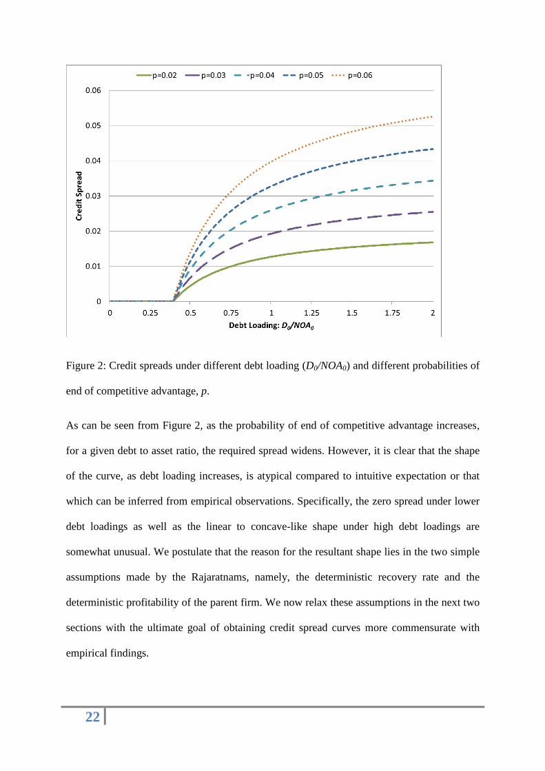
3.5.2 Yield curve covering only default risk under different debt loadings

In this section we fix maturity at N=10 years, the recovery rate at f=40%, and note that the

comparable 10 year Gilt trades at a yield of 2.34%. We then plot the credit spread for the

firm’s debt for different debt to asset ratios and under five different probability of end of

competitive advantage p ϵ {0.02, 0.03, 0.04, 0.05, 0.06}.

22

Figure 2: Credit spreads under different debt loading (D0/NOA0) and different probabilities of

end of competitive advantage, p.

As can be seen from Figure 2, as the probability of end of competitive advantage increases,

for a given debt to asset ratio, the required spread widens. However, it is clear that the shape

of the curve, as debt loading increases, is atypical compared to intuitive expectation or that

which can be inferred from empirical observations. Specifically, the zero spread under lower

debt loadings as well as the linear to concave-like shape under high debt loadings are

somewhat unusual. We postulate that the reason for the resultant shape lies in the two simple

assumptions made by the Rajaratnams, namely, the deterministic recovery rate and the

deterministic profitability of the parent firm. We now relax these assumptions in the next two

sections with the ultimate goal of obtaining credit spread curves more commensurate with

empirical findings.

23

4. Type II: Firm valuation model with deterministic profitability and

non-deterministic recovery.

In this section, we relax the assumption of deterministic recovery.

4.1 Unlevered Firm Valuation model under non-deterministic recovery

Assumptions 1-5 from section 3.1 apply but assumption 6 is modified as follows:

6. When competitive advantage is lost in some future year i, the earnings potential of the

business is fully impaired and it is liquidated in the same year. In section 3.1, we assumed

that the liquidation value in year i is a constant fraction f≤1 of the Net Operating Assets in

year i. A constant recovery fraction, as an assumption, though uncontroversial in theory is

rather unhelpful in practice. Liquidation values are highly uncertain. They depend on a

variety of factors including macro-economic / monetary conditions, degree of excess

capacity in the sector where the firm participates, rational and opportunistic behavior by

various stakeholders as well as time value leakage when proceedings are drawn out. We

now assume that the asset recovery ratio is a random variable with a maximum f≤1 of the

Net Operating Assets and the following simple monomial pdf of kth

degree:

ℎ(𝑥) =𝑘+1

𝑓𝑘+1𝑥𝑘 𝑓𝑜𝑟 0 ≤ 𝑥 ≤ 𝑓, 𝑘 ≥ 0 (20)

Note that in our model, we still assume that when competitive advantage is lost, the

impact is rapidly felt on the economics of the business within the year rather than drawn

out over many years: unknowns like potential time-value leakage and other leakages

being captured by a judicious choice of f and k.

The expected present-valued cash flows that accrue to an equity holder in the unlevered firm

in scenario i (where competitive advantage lasts up to year i) is given by:

𝑉𝑖 = (∑𝑁𝑂𝐴0 (𝑅𝑂𝑁𝑂𝐴 − 𝑔 )(1+𝑔)𝑗

(1+𝑟𝑊)𝑗𝑖𝑗=1 ) + ∫

𝑘+1

𝑓𝑘+1 𝑥𝑘+1 𝑁𝑂𝐴0(1+𝑔)𝑖+1

(1+𝑟𝑊)𝑖+1 𝑑𝑥 𝑓

0 (21)

24

𝑉𝑖 = (∑𝑁𝑂𝐴0 (𝑅𝑂𝑁𝑂𝐴 − 𝑔 )(1+𝑔)𝑗

(1+𝑟𝑊)𝑗𝑖𝑗=1 ) + [

(𝑘+1)𝑓

𝑘+2]

𝑁𝑂𝐴0(1+𝑔)𝑖+1

(1+𝑟𝑊)𝑖+1 (22)

The only difference between the above equation and eqn. (4) is that the deterministic asset

recovery factor f has been replaced with the mean of the pdf given by eqn. (20). Equation

(22) equals equation (4) as k grows without bound and the probability density function

becomes the impulse function. The expected inherent value of the firm, MF, can be

determined using the identities in Appendix A:

𝑀𝐹 = ∑ 𝑃𝑖𝑉𝑖∞𝑖=0 =

𝑁𝑂𝐴0 (𝑅𝑂𝑁𝑂𝐴 − 𝑔 ) ( 1−𝑝 )( 1+𝑔 )

𝑟𝑊+ 𝑝−𝑔+𝑝𝑔 + [

(𝑘+1)𝑓

𝑘+2]

𝑁𝑂𝐴0 𝑝(1+𝑔)

𝑟𝑊+ 𝑝−𝑔+𝑝𝑔 (23)

Armed with the approximate probability distribution11

of present values described in Eqs (1)

and (22), a value investor may allocate a portion of her capital to the firm using the capital

allocation methodology provided by the Rajaratnams.

4.2 Debt Valuation model under non-deterministic recovery

Assumptions 7-9 from section 3.2 apply. Equations (8) and (9) for Ci are valid for the

expected sum of all the discounted coupons and principal in outcome i that is paid to debt-

holders with vintage (0), assuming that competitive advantage ends in year i+1. However,

instead of equations (10) and (11) from the deterministic recovery scenario, the new expected

recovery values Ri+1 in year i+1 are:

[1] For D0(1+y) ≤ fNOA0:

𝑅𝑖+1 =(𝑆0+𝑦𝑆0)𝑁𝑂𝐴𝑖+1

𝐷𝑖+1(1+𝑦)[∫

𝑘+1

𝑓𝑘+1 𝑥𝑘+1 𝑑𝑥 +

𝐷𝑖+1+𝑦𝐷𝑖+1𝑁𝑂𝐴𝑖+1

0∫

𝐷𝑖+1(1+𝑦)(𝑘+1)

𝑁𝑂𝐴𝑖+1𝑓𝑘+1 𝑥𝑘 𝑑𝑥 𝑓

𝐷𝑖+1+𝑦𝐷𝑖+1𝑁𝑂𝐴𝑖+1

] (24)

11

The expression is only an approximation from a value-investor point of view given that the variability in

recovery would require some form of risk adjustment for specifically recovery related cash flows in year i+1.

However, for the purposes of this paper, we assume that the approximation suffices. As suggested by the

Rajaratnams, the fractional Kelly system is available for use in the Capital Allocation model in such instances.

25

= 𝑆0 ((1 + 𝑦) −𝐷0

𝑘+1(1+𝑦)𝑘+2

(𝑘+2)𝑁𝑂𝐴0𝑘+1𝑓𝑘+1 ) (25)

[2] For D0 (1+y) > fNOA0:

𝑅𝑖+1 =(𝑆0+𝑦𝑆0)𝑁𝑂𝐴𝑖+1

𝐷𝑖+1(1+𝑦)∫

𝑘+1

𝑓𝑘+1 𝑥𝑘+1 𝑑𝑥 𝑓

0 (26)

=𝑆0𝑁𝑂𝐴0

𝐷0 [

(𝑘+1)𝑓

𝑘+2] (27)

The expected inherent-value MSo of all the discounted coupons and principal that is received

by the debt-holder can be calculated (with the help of the identities in Appendix A) as:

[1] For D0(1+y) ≤ fNOA0:

𝑀𝑆𝑜 = ∑ 𝑃𝑖𝐷𝐶𝑖

𝑁𝑖=0 =

𝑆0

𝑟𝑁+𝑝(𝑦(1 − 𝑝) + 𝑝 ((1 + 𝑦) −

𝐷0𝑘+1(1+𝑦)𝑘+2

(𝑘+2)𝑁𝑂𝐴0𝑘+1𝑓𝑘+1 )) (1 −

(1−𝑝)𝑁

(1+𝑟𝑁)𝑁) +

+ 𝑆0(1−𝑝)𝑁

(1+𝑟𝑁)𝑁 (28)

[2] For D0(1+y) > fNOA0:

𝑀𝑆𝑜 = ∑ 𝑃𝑖𝐷𝐶𝑖

𝑁𝑖=0 = 𝑆0

𝑦(1−𝑝)+[(𝑘+1)𝑓

𝑘+2]𝑝

𝑁𝑂𝐴0𝐷0

𝑟𝑁+𝑝(1 −

(1−𝑝)𝑁

(1+𝑟𝑁)𝑁) + 𝑆0(1−𝑝)𝑁

(1+𝑟𝑁)𝑁 (29)

The annual probability of default in this model, PD=p[D0(1+y)/(fNOA0)]k+1

for D0(1+y) ≤

fNOA0. For D0(1+y) > fNOA0, the annual probability of default is the same as the annual

probability of end of competitive advantage, PD=p. Thereafter, it is straightforward to obtain

the cumulative probability of default in either case given that the annual default events are

identical in each year.

One can also derive the expected inherent value, ME, for an equity holder in the firm. From

an equity holder’s point of view, Eqn (1) still applies for the probability, Pi. The expected

present valued cash flows, Vi, that accrues to the shareholder:

26

𝑉𝑖 = (∑𝑁𝑂𝐴0 (𝑅𝑂𝑁𝑂𝐴 − 𝑔 )(1+𝑔)𝑗−𝐷0(𝑦(1−𝑇)−𝑔)(1+𝑔)𝑗

(1+𝑟𝑊)𝑗𝑖𝑗=1 ) +

𝐿(1+𝑔)𝑖+1

(1+𝑟𝑊)𝑖+1 (30)

where L represents what is left over from the recovery (if any) after debt holders get what is

owed to them:

𝐿 = (𝑘+1)𝑓𝑁𝑂𝐴0

𝑘+2− 𝐷0(1 + 𝑦) +

𝐷0𝑘+2(1+𝑦)𝑘+2

(𝑘+2)𝑁𝑂𝐴0𝑘+1𝑓𝑘+1 𝑓𝑜𝑟 𝐷0(1 + 𝑦) ≤ 𝑓𝑁𝑂𝐴0 (31)

𝐿 = 0 𝑓𝑜𝑟 𝐷0(1 + 𝑦) > 𝑓𝑁𝑂𝐴0 (32)

Thereafter the expected inherent value of the equity, ME:

𝑀𝐸 = ∑ 𝑃𝑖𝑉𝑖∞𝑖=0 =

[𝑁𝑂𝐴0(𝑅𝑂𝑁𝑂𝐴 −𝑔)−𝐷0(𝑦(1−𝑇)−𝑔)]( 1−𝑝 )( 1+𝑔 ) + 𝐿𝑝(1+𝑔)

𝑟𝑊+ 𝑝−𝑔+𝑝𝑔 (33)

4.3 Term structure of corporate credit for non-deterministic recovery

Similar to section 3.3, to derive the term structure rate (covering only default risk) y* which

would make a risk-neutral investor indifferent between the debt security issued at par value

and the risk free asset, we simply set, MSo = S0 in equations (28) and (29) and solve for y*:

1 + 𝑟𝑁 = (1 + 𝑦∗) − (1+𝑦∗)𝑘+2

𝑘+2

𝑝𝐷0𝑘+1

(𝑓𝑁𝑂𝐴0)𝑘+1 𝑓𝑜𝑟 𝐷0(1 + 𝑦∗) ≤ 𝑓𝑁𝑂𝐴0 (34)

𝑦∗ =𝑟𝑁+𝑝−𝑝

𝑁𝑂𝐴0𝐷0

[(𝑘+1)𝑓

𝑘+2]

1−𝑝 𝑓𝑜𝑟 𝐷0(1 + 𝑦∗) > 𝑓𝑁𝑂𝐴0 (35)

Although equation (35) is explicitly solved for the term structure, equation (34) does not

appear to be solvable algebraically (other than for small integral values of k, in which case

the standard expressions for solving quadratic equations and slightly higher order

polynomials become useful). Nevertheless equation (34), which has the depressed polynomial

structure xk+2

+a1x+a0=0 where a0 and a1 are constants, is not difficult to solve using simple

spreadsheets such as Excel for k>0. Note that equations (34) and (35) result in equations (16)

and (17) as k grows without bound and the pdf becomes an impulse function. The curve

27

obtained by joining equations (34) and (35) at the point D0(1+y*) = fNOA0 is continuous as

both equations converge to the same value y*=[rN+p/(k+2)]/[1-p/(k+2)] at this point.

Using a similar argument as in section 3.4, we can then determine the actual spread that can

be offered to the debt holder to compensate for more than just expected default loss (based on

a fair apportionment of the transferred tax wealth) using equation (19).

4.4 Term structure results for type II models

4.4.1 Risk neutral term structure covering only default risk

For the risk free yield curve, we employ a snapshot of the latest UK Gilt yield curve. We

consider a target debt to asset ratio, D0/NOA0 = 60% and a probability of end of competitive

advantage, p=0.05. We then plot the term structure for the firm’s debt under two different

recovery factors f ϵ {30%, 60%} and four different monomial pdf degree factors k ϵ {1, 2, 5,

∞}. Note that scenario k = ∞ in type II models is identical to type I models.

28

Figure 3: The term structure of corporate credit for different asset recovery factors, f, and

different degree factors, k, of the monomial pdf that represents the recovery process.

As can be seen, as the recovery rate reduces, the required spread widens. As can also be seen,

for a given asset recovery factor, the required spread increases with decreasing monomial pdf

degree factors. This is intuitive: as one decreases the degree factor in equation (20), the

expected recovery reduces and therefore the required spread widens. Once again, the

proposed model seems to be able to predict a wide array of spreads ranging from wider

spreads for lower grade firms (having lower recovery rates) to narrower spreads for higher

grade firms (having higher recovery rates).

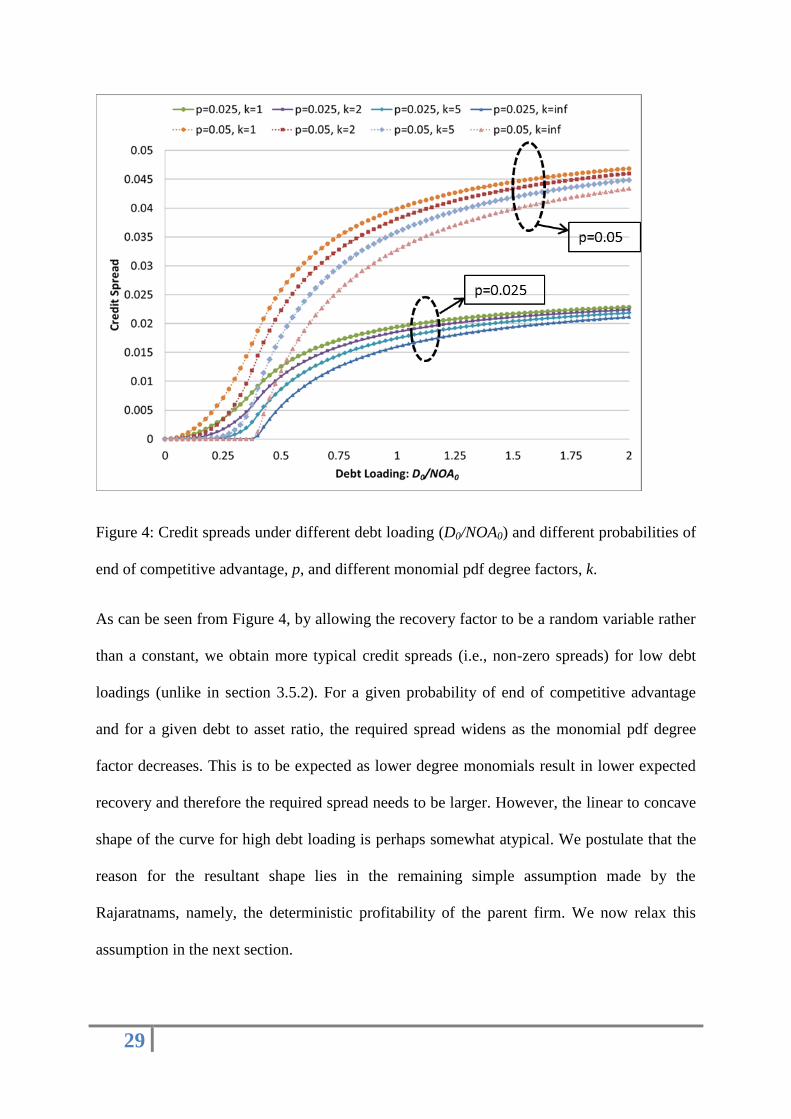
4.4.2 Yield curve covering only default risk under different debt loadings

Similar to section 3.5.2, we fix maturity at N=10 years, the recovery rate at f=40%, and note

that the comparable 10 year Gilt trades at a yield of 2.34%. We then plot the credit spread for

the firm’s debt for different debt to asset ratios and under two different probability of end of

competitive advantage p ϵ {0.025, 0.05} and four different monomial pdf degree factors k ϵ

{1, 2, 5, ∞}.

29

Figure 4: Credit spreads under different debt loading (D0/NOA0) and different probabilities of

end of competitive advantage, p, and different monomial pdf degree factors, k.

As can be seen from Figure 4, by allowing the recovery factor to be a random variable rather

than a constant, we obtain more typical credit spreads (i.e., non-zero spreads) for low debt

loadings (unlike in section 3.5.2). For a given probability of end of competitive advantage

and for a given debt to asset ratio, the required spread widens as the monomial pdf degree

factor decreases. This is to be expected as lower degree monomials result in lower expected

recovery and therefore the required spread needs to be larger. However, the linear to concave

shape of the curve for high debt loading is perhaps somewhat atypical. We postulate that the

reason for the resultant shape lies in the remaining simple assumption made by the

Rajaratnams, namely, the deterministic profitability of the parent firm. We now relax this

assumption in the next section.

30

5. Type III: Firm valuation model with non-deterministic profitability

and non-deterministic recovery.

5.1 Unlevered Firm Valuation model

We now consider a model for an unlevered firm under both non-deterministic profitability

and non-deterministic recovery. In sections 3 and 4, the return on net operating assets,

RONOA, was constant but, importantly, large enough to ensure that all coupons prior to the

loss of competitive advantage were honored. In this section, we relax this assumption to

introduce uncertainty in the honoring of coupons prior to the loss of competitive advantage.

There are numerous ways to do so but most avenues of attack on this problem quickly lead to

intractable expressions. In this first exposition linking term structure to competitive

advantage, we have opted for simple but reasonable assumptions, ones that allow us to limit

the burden on mathematical tractability but still introduce the essence of coupon uncertainty

prior to loss of competitive advantage.

We take that assumptions 1, 2, 4 and 5 from section 3 as well as assumption 6 (regarding

non-deterministic recovery) from section 4 apply. However, assumption 3 from section 3 is

modified as follows:

3. The original assumption was that whilst its competitive advantage is sustained, the firm

earns a constant Return on Net-Operating Assets (that is, a constant RONOA). We relax

this assumption in the following manner: We allow the sustainable (through the cycle)

return on net operating assets that the firm earns to be a random variable, ronoa, with a

symmetrical truncated normal distribution with mean and standard deviation (t,t). More

technically, we consider a parent (untruncated) normal distribution with parameters (,)

31

where =RONOA and truncate12

it at the lower boundary rW and the upper boundary

2RONOA- rW. The mean of the resulting truncated distribution is t =RONOA. Any

standard graduate statistics textbook should show how explicit relationships for the

standard deviation t, the pdf. t and the cdf. t of the truncated normal distribution can

be obtained from the parameters (,, rW, 2RONOA- rW). With our stated intent of limiting

the burden on mathematical tractability, we also make the simple assumption that at the

beginning of year 1, ronoa is drawn from the above mentioned truncated pdf and

sustained at that level over time until competitive advantage ends. As before, we assume

that the unlevered firm grows its profits and asset base at a constant annual growth rate of

g under these assumptions.

The expected present-valued cash flows that accrue to an equity holder in the unlevered firm

in scenario i (where competitive advantage lasts up to year i) is given by:

𝑉𝑖 = (∑𝑁𝑂𝐴0 (1+𝑔)𝑗

(1+𝑟𝑊)𝑗𝑖𝑗=1 ((∫ 𝑥 ∅𝑡(𝑥; ,, 𝑟𝑊, 2𝑅𝑂𝑁𝑂𝐴 − 𝑟𝑊)𝑑𝑥

2𝑅𝑂𝑁𝑂𝐴−𝑟𝑊

𝑟𝑊) − 𝑔)) +

+ ∫ 𝑘+1

𝑓𝑘+1 𝑥𝑘+1 𝑁𝑂𝐴0(1+𝑔)𝑖+1

(1+𝑟𝑊)𝑖+1 𝑑𝑥𝑓

0 (36)

𝑉𝑖 = (∑𝑁𝑂𝐴0 (𝑡 − 𝑔 )(1+𝑔)𝑗

(1+𝑟𝑊)𝑗𝑖𝑗=1 ) + [

(𝑘+1)𝑓

𝑘+2]

𝑁𝑂𝐴0(1+𝑔)𝑖+1

(1+𝑟𝑊)𝑖+1 (37)

The only difference between eqn. (22) and the above equation is that the deterministic

RONOA has been replaced with the mean of the truncated normal pdf, t =RONOA. Equation

(36) becomes (21) as the standard deviation of the truncated normal distribution tends to zero.

The expected inherent value of the firm, MF, can be determined using the identities in

Appendix A:

12

Note that the derivation that follows is not much more complicated if we choose any other equidistant

boundaries from the mean of the parent normal distribution.

32

𝑀𝐹 = ∑ 𝑃𝑖𝑉𝑖∞𝑖=0 =

𝑁𝑂𝐴0 (𝑡− 𝑔 ) ( 1−𝑝 )( 1+𝑔 )

𝑟𝑊+ 𝑝−𝑔+𝑝𝑔 + [

(𝑘+1)𝑓

𝑘+2]

𝑁𝑂𝐴0 𝑝(1+𝑔)

𝑟𝑊+ 𝑝−𝑔+𝑝𝑔 (38)

Armed with the (approximate) probability distribution of present values described by Eqs (1)

and (37), a value investor may allocate a portion of her capital to the firm using the capital

allocation methodology provided by the Rajaratnams.

5.2 Debt Valuation model under non-deterministic recovery and profitability

The main complication now is that (unlike in section 3.2 and 4.2), ronoa is a random variable

and this can lead to two distinct scenarios. Scenario A1 is one which is constructive for debt

holders in that profits (ronoa) is sufficient to pay coupons. Scenario A1 is identical to the

scenario described in section 4.2 in relation to growth capex, dividend and coupon payments,

new debt issues and principal repayments, as well as liquidation and recovery13

. On the other

hand, scenario A2 is negative for debt holders (and downright destructive for shareholders) in

that the firm is in financial distress: ronoa is not sufficient to pay coupons. In scenario A2, we

assume that dividends, growth capex, new debt issues and principal repayments are all

suspended. In this distress scenario, we assume that shareholders end up with nothing and

play no further part in the firm. Debt holders share whatever pre-tax profits the firm makes in

proportion to the outstanding principal. In scenario A2, if competitive advantage is lost before

maturity of N years, then liquidation and recovery is non-deterministic as per section 4.2; the

only difference is that in this scenario debt holders share the full liquidation proceeds in

proportion to outstanding principal (and shareholders get nothing). If, on the other hand,

competitive advantage is maintained with probability (1-p)N until maturity of N years, then

the firm is sold as a going concern to a trade buyer (a consolidator in the industry for whom

13

If there is not enough cash flows (after payment of coupons) for the firm to grow at rate g, the firm is assumed

to issue sufficient small amounts of equity to shareholders to fund growth capex.

33

there are potential untapped cost savings / synergies) for a price equal to the total outstanding

principal obligations owed to the debt holders.

We now define RONOA* as that particular ronoa from the truncated normal distribution

above which scenario A1 occurs and below which scenario A2 occurs. RONOA* can be easily

obtained by setting the post-tax earnings (prior to loss of competitive advantage) equal to the

tax-deductible coupon in period 1:

𝑁𝑂𝐴0 𝑅𝑂𝑁𝑂𝐴∗ (1 + 𝑔) − 𝐷0𝑦(1 − 𝑇)(1 + 𝑔) = 0 (39)

𝑅𝑂𝑁𝑂𝐴∗ =𝐷0

𝑁𝑂𝐴0𝑦(1 − 𝑇) (40)

We now define Q as the cumulative probability of scenario A2. The probability of scenario A1

is therefore (1-Q). The probability Q is obtained from the cdf. of the truncated normal

distribution at RONOA*:

𝑄 = 𝑡(𝑅𝑂𝑁𝑂𝐴∗; ,, 𝑟𝑊, 2𝑅𝑂𝑁𝑂𝐴 − 𝑟𝑊) (41)

Define Ci as the expected sum of all the discounted coupons and principal in outcome i that is

paid to debt-holders with vintage (0), assuming that competitive advantage ends in year i+1.

Defining z to be the scenario dependent coupon rate that is a random variable and then using

the expression for total expectation in terms of conditional expectations:

𝐶0 =(1−𝑄)𝐸[𝑅1/𝐴1]

(1+𝑟𝑁)+

𝑄𝐸[𝑅1/𝐴2]

(1+𝑟𝑁) (42)

For 0<i<N:

𝐶𝑖 = (∑(1−𝑄)𝐸[𝑧/𝐴1]𝑆0

(1+𝑟𝑁)𝑗𝑖𝑗=1 ) +

(1−𝑄)𝐸[𝑅𝑖+1/𝐴1]

(1+𝑟𝑁)𝑖+1+ (∑

𝑄𝐸[𝑧/𝐴2]𝑆0

(1+𝑟𝑁)𝑗𝑖𝑗=1 ) +

𝑄𝐸[𝑅𝑖+1/𝐴2]

(1+𝑟𝑁)𝑖+1 (43)

𝐶𝑁 = (∑(1−𝑄)𝐸[𝑧/𝐴1]𝑆0

(1+𝑟𝑁)𝑗𝑁𝑗=1 ) +

(1−𝑄)𝑆0

(1+𝑟𝑁)𝑁+ (∑

𝑄𝐸[𝑧/𝐴2]𝑆0

(1+𝑟𝑁)𝑗𝑁𝑗=1 ) +

𝑄𝑆0

(1+𝑟𝑁)𝑁 (44)

34

where E[x/Ai] denotes the conditional expectation of x given scenario Ai and

𝐸[𝑧/𝐴1] = 𝑦 (45)

𝐸[𝑧/𝐴2] =𝑁𝑂𝐴0

𝑄𝐷0(1−𝑇)(∫ 𝑥∅𝑡(𝑥; ,, 𝑟𝑊, 2𝑅𝑂𝑁𝑂𝐴−𝑟𝑊)𝑑𝑥

𝑅𝑂𝑁𝑂𝐴∗

𝑟𝑊) (46)

𝐸[𝑧/𝐴2] =𝑁𝑂𝐴0

𝐷0(1−𝑇){ −

(0,1;𝑅𝑂𝑁𝑂𝐴∗−

)−(0,1;

𝑟𝑤−

)

(0,1;𝑅𝑂𝑁𝑂𝐴∗−

)−(0,1;

𝑟𝑤−

)} (47)

where (0,1;x) and (0,1;x) are the pdf. and cdf. of the standard normal distribution with

mean 0 and standard deviation 1 respectively. The expression in curly brackets in eqn (47) is

the mean of a truncated normal distribution obtained by truncating the parent normal

distribution with parameters (, ) at the lower end rW and at the upper end RONOA*.

Expected liquidation proceeds conditional on scenario A1 can be obtained following the same

derivation as section 4.2:

𝐸[𝑅𝑖+1/𝐴1] = 𝑆0 ((1 + 𝑦) −𝐷0

𝑘+1(1+𝑦)𝑘+2

(𝑘+2)𝑁𝑂𝐴0𝑘+1𝑓𝑘+1 ) 𝑓𝑜𝑟 𝐷0(1 + 𝑦) ≤ 𝑓𝑁𝑂𝐴0 (48)

𝐸[𝑅𝑖+1/𝐴1] =𝑆0𝑁𝑂𝐴0

𝐷0 [

(𝑘+1)𝑓

𝑘+2] 𝑓𝑜𝑟 𝐷0(1 + 𝑦) > 𝑓𝑁𝑂𝐴0 (49)

Expected liquidation proceeds conditional on scenario A2:

𝐸[𝑅𝑖+1/𝐴2] =𝑆0𝑁𝑂𝐴0

𝐷0 [

(𝑘+1)𝑓

𝑘+2] (50)

The expected inherent-value MSo of all the discounted coupons and principal that is received

by the debt-holder can be calculated (with the help of the identities in Appendix A) as:

[1] For D0(1+y) ≤ fNOA0:

35

𝑀𝑆𝑜 = 𝑆0(1 − 𝑄)

𝑟𝑁+𝑝(𝑦(1 − 𝑝) + 𝑝 ((1 + 𝑦) −

𝐷0𝑘+1(1+𝑦)𝑘+2

(𝑘+2)𝑁𝑂𝐴0𝑘+1𝑓𝑘+1 )) (1 −

(1−𝑝)𝑁

(1+𝑟𝑁)𝑁) +

+ 𝑆0𝑄

𝑟𝑁+𝑝(𝐸[𝑧/𝐴2](1 − 𝑝) + [

(𝑘+1)𝑓

𝑘+2] 𝑝

𝑁𝑂𝐴0

𝐷0 ) (1 −

(1−𝑝)𝑁

(1+𝑟𝑁)𝑁) + 𝑆0(1−𝑝)𝑁

(1+𝑟𝑁)𝑁 (51)

[2] For D0(1+y) > fNOA0:

𝑀𝑆𝑜 = 𝑆0(1−𝑄)

𝑟𝑁+𝑝(𝑦(1 − 𝑝) + [

(𝑘+1)𝑓

𝑘+2] 𝑝

𝑁𝑂𝐴0

𝐷0) (1 −

(1−𝑝)𝑁

(1+𝑟𝑁)𝑁) + 𝑆0𝑄

𝑟𝑁+𝑝(𝐸[𝑧/𝐴2](1 − 𝑝) +

+ [(𝑘+1)𝑓

𝑘+2] 𝑝

𝑁𝑂𝐴0

𝐷0 ) (1 −

(1−𝑝)𝑁

(1+𝑟𝑁)𝑁) + 𝑆0(1−𝑝)𝑁

(1+𝑟𝑁)𝑁 (52)

where E[z/A2] is given by eqn (47).

It is not difficult to see that as the standard deviation of the original pdf tends to zero, Q tends

to 0 and equations (51-52) tend to equations (28-29) respectively. It is also not that difficult

to show that the cumulative probability of default, CPD, for vintage (0), CPD=Q+(1-Q)(1-

{1-p[D0(1+y)/(fNOA0)]k+1

}N) for D0(1+y) ≤ fNOA0. For D0(1+y) > fNOA0, CPD=Q+(1-Q)(1-

{1-p}N).

One can also derive the expected inherent value, ME, for an equity holder in the firm. From

an equity holder’s point of view, Eqn (1) still applies for the probability, Pi. The expected

present valued cash flows, Vi, that accrues to the shareholder in scenario i:

𝑉𝑖 = (1 − 𝑄) [(∑𝑁𝑂𝐴0 (𝐸[𝑟𝑜𝑛𝑜𝑎/𝐴1] − 𝑔 )(1+𝑔)𝑗−𝐷0(𝑦(1−𝑇)−𝑔)(1+𝑔)𝑗

(1+𝑟𝑊)𝑗𝑖𝑗=1 ) +

𝐿(1+𝑔)𝑖+1

(1+𝑟𝑊)𝑖+1] (53)

𝐸[𝑟𝑜𝑛𝑜𝑎/𝐴1] = ( − (0,1;

2𝑅𝑂𝑁𝑂𝐴−𝑟𝑤−

)−(0,1;

𝑅𝑂𝑁𝑂𝐴∗−

)

(0,1;2𝑅𝑂𝑁𝑂𝐴−𝑟𝑤−

)−(0,1;

𝑅𝑂𝑁𝑂𝐴∗−

)) (54)

where L represents what is left over from the recovery (if any) after debt holders get what is

owed to them (and is identical to section 4.2):

𝐿 = (𝑘+1)𝑓𝑁𝑂𝐴0

𝑘+2− 𝐷0(1 + 𝑦) +

𝐷0𝑘+2(1+𝑦)𝑘+2

(𝑘+2)𝑁𝑂𝐴0𝑘+1𝑓𝑘+1

𝑓𝑜𝑟 𝐷0(1 + 𝑦) ≤ 𝑓𝑁𝑂𝐴0 (55)

36

𝐿 = 0 𝑓𝑜𝑟 𝐷0(1 + 𝑦) > 𝑓𝑁𝑂𝐴0 (56)

Thereafter the expected inherent value of the equity, ME:

𝑀𝐸 = ∑ 𝑃𝑖𝑉𝑖∞𝑖=0 = (1 − 𝑄)

[𝑁𝑂𝐴0 (𝐸[𝑟𝑜𝑛𝑜𝑎/𝐴1] − 𝑔 )−𝐷0(𝑦(1−𝑇)−𝑔)]( 1−𝑝 )( 1+𝑔 ) + 𝐿𝑝(1+𝑔)

𝑟𝑊+ 𝑝−𝑔+𝑝𝑔 (57)

5.3 Term structure of corporate credit for non-deterministic profitability

Similar to section 3.3, to derive the term structure rate y* (covering only default risk) which

would make a risk-neutral investor indifferent between the debt security issued at par value

and the risk free asset, one simply sets, MSo = S0 in equations (51) and (52) and solve for y*:

[1] For D0(1+y*) ≤ fNOA0:

𝑟𝑁 + 𝑝 =

(1 − 𝑄) ((𝑝 + 𝑦∗) − (1+𝑦∗)𝑘+2

𝑘+2

𝑝𝐷0𝑘+1

(𝑓𝑁𝑂𝐴0)𝑘+1) + 𝑄 (𝐸[𝑧/𝐴2](1 − 𝑝) + [

(𝑘+1)𝑓

𝑘+2] 𝑝

𝑁𝑂𝐴0

𝐷0 ) (58)

[2] For D0(1+y*) > fNOA0:

𝑦∗ =𝑟𝑁+𝑝−𝑝

𝑁𝑂𝐴0𝐷0

[(𝑘+1)𝑓

𝑘+2]−𝑄(𝐸[𝑧/𝐴2](1−𝑝) )

(1−𝑝)(1−𝑄) (59)

Both equations are no longer solvable algebraically but are quite amenable to solution using

simple spreadsheets such as Excel. Note that equations (58) and (59) result in equations (34)

and (35) as the standard deviation of the truncated normal pdf tends to zero. Both equations

meet at the same point when D0(1+y*) = fNOA0 to form a continuous line. Using a similar

argument as in section 3.4, we can then determine the actual spread that can be offered to the

debt holder to compensate for more than just expected default loss (based on a fair

apportionment of the transferred tax wealth) using equation (19).

37

5.4 Term structure results for type III models

5.4.1 Risk neutral term structure covering only default risk

We consider a target debt to asset ratio, D0/NOA0 = 60% and a probability of end of

competitive advantage, p=0.05. We then plot the term structure for the firm’s debt under two

different recovery factors f ϵ {30%, 60%}, four different monomial pdf degree factors k ϵ {1,

2, 5, ∞} and under a coefficient of variation (CV) of the parent normal distribution for ronoa,

CV = / = 0.5.

Figure 5: The term structure of corporate credit for different recovery factors, f, different

degree factors, k, of the monomial pdf that represents the recovery process and a variable

ronoa

As can be seen, as the recovery rate reduces, the required spread widens. As can also be seen,

for a given recovery factor, the required spread increases with decreasing monomial pdf

38

degree factors. The proposed model seems to be able to predict a wide array of spreads

ranging from wider spreads for lower grade firms (having lower recovery rates) to narrower

spreads for higher grade firms (having higher recovery rates). In figure 5, we consider only a

single coefficient of variation. In the next section we consider a wider range for the

coefficient of variation of the parent distribution.

5.4.2 Yield curve covering only default risk under different debt loadings

Similar to section 4.4.2, we fix maturity at N=10 years, the recovery rate at f=40%, and note

that the comparable 10 year Gilt trades at a yield of 2.34%. We then plot the credit spread for

the firm’s debt for different debt to asset ratios, under k = 2, under two different probability

of end of competitive advantage p ϵ {0.025, 0.05} and where the CV the coefficient of

variation of the parent normal distribution for RONOA ranges from 0 to 1.

Figure 6: Credit spreads under different debt loading (D0/NOA0) and different probabilities of

end of competitive advantage, p, and different coefficient of variations, CV.

39

As can be seen from Figure 6, by allowing both the recovery factor and the return of net

operating assets, ronoa, to be random variables rather than constants, we obtain more typical

convex shaped credit spreads for very high debt loadings. For a given probability of end of

competitive advantage and for a given debt to asset ratio, the required spread widens as the

coefficient of variation increases. This is to be expected as higher variation in ronoa leads to

a larger probability of coupons not being honored and therefore the required spread needs to

be larger.

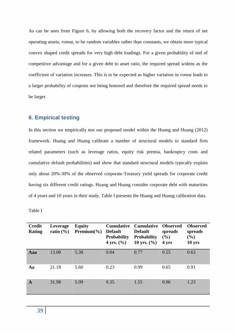
6. Empirical testing

In this section we empirically test our proposed model within the Huang and Huang (2012)

framework. Huang and Huang calibrate a number of structural models to standard firm

related parameters (such as leverage ratios, equity risk premia, bankruptcy costs and

cumulative default probabilities) and show that standard structural models typically explain

only about 20%-30% of the observed corporate-Treasury yield spreads for corporate credit

having six different credit ratings. Huang and Huang consider corporate debt with maturities

of 4 years and 10 years in their study. Table I presents the Huang and Huang calibration data.

Table I

Credit

Rating

Leverage

ratio (%)

Equity

Premium(%)

Cumulative

Default

Probability

4 yrs. (%)

Cumulative

Default

Probability

10 yrs. (%)

Observed

spreads

(%)

4 yrs

Observed

spreads

(%)

10 yrs

Aaa 13.08 5.38 0.04 0.77 0.55 0.63

Aa 21.18 5.60 0.23 0.99 0.65 0.91

A 31.98 5.99 0.35 1.55 0.96 1.23

40

Baa 43.28 6.55 1.24 4.39 1.58 1.94

Ba 53.53 7.30 8.51 20.63 3.20 3.20

B 65.70 8.76 23.32 43.91 4.70 4.70

This table shows the target parameters for calibration and the historical average corporate-

treasury yield spreads for each credit rating group from Huang and Huang (2012).

6.1 Calibration exercise

We calibrate our type II model to the Huang and Huang (2012) framework14

in an

approximate fashion. In our type II models, the following parameters need to be determined:

leverage ratio, D0/NOA0, probability of end of competitive advantage, p, asset recovery ratio,

f, and monomial degree factor, k. We use the same leverage ratio as that given by Huang and

Huang. We employ the same bankruptcy costs (15%) as suggested by them and set our asset

recovery factor f=85% for all credit ratings. As we show in appendix B, we infer from the

equity risk premium the probability parameter, p. Finally, we convert the cumulative default

probabilities provided by Huang and Huang into annual probabilities of default and then from

our expressions for annual default probabilities we solve for the monomial degree factor, k.

Note that our expressions for annual default probabilities require an estimate of the coupon

rate, y, therefore we solve for, k, and calculate, y, (equation 19) in an iterative manner. The

average 10-year treasury rate for the period specified by Huang and Huang (2012) was

obtained from the St. Louis Federal Reserve data series. The average 4-year treasury rate was

also obtained from the same source by simply averaging the 3-year and 5-year treasury yield

data series for the period specified by Huang and Huang.

14

Our type I model is far too simplistic and is under parameterized. Our type III model can be calibrated to

Huang and Huang but it is over parameterized – it has more parameters than is necessary to calibrate. Anyway,

our type II model is simply our type III model with coefficient of variation equal to zero.

41

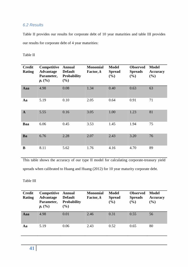
6.2 Results

Table II provides our results for corporate debt of 10 year maturities and table III provides

our results for corporate debt of 4 year maturities:

Table II

Credit

Rating

Competitive

Advantage

Parameter,

p, (%)

Annual

Default

Probability

(%)

Monomial

Factor, k

Model

Spread

(%)

Observed

Spreads

(%)

Model

Accuracy

(%)

Aaa 4.98 0.08 1.34 0.40 0.63 63

Aa 5.19 0.10 2.05 0.64 0.91 71

A 5.55 0.16 3.05 1.00 1.23 81

Baa 6.06 0.45 3.53 1.45 1.94 75

Ba 6.76 2.28 2.07 2.43 3.20 76

B 8.11 5.62 1.76 4.16 4.70 89

This table shows the accuracy of our type II model for calculating corporate-treasury yield

spreads when calibrated to Huang and Huang (2012) for 10 year maturity corporate debt.

Table III

Credit

Rating

Competitive

Advantage

Parameter,

p, (%)

Annual

Default

Probability

(%)

Monomial

Factor, k

Model

Spread

(%)

Observed

Spreads

(%)

Model

Accuracy

(%)

Aaa 4.98 0.01 2.46 0.31 0.55 56

Aa 5.19 0.06 2.43 0.52 0.65 80

42

A 5.55 0.09 3.62 0.81 0.96 84

Baa 6.06 0.31 4.01 1.17 1.58 74

Ba 6.76 2.20 2.02 2.09 3.20 65

B 8.11 6.42 0.66 5.01 4.70 107

This table shows the accuracy of our type II model for calculating corporate-treasury yield

spreads when calibrated to Huang and Huang (2012) for 4 year maturity corporate debt.

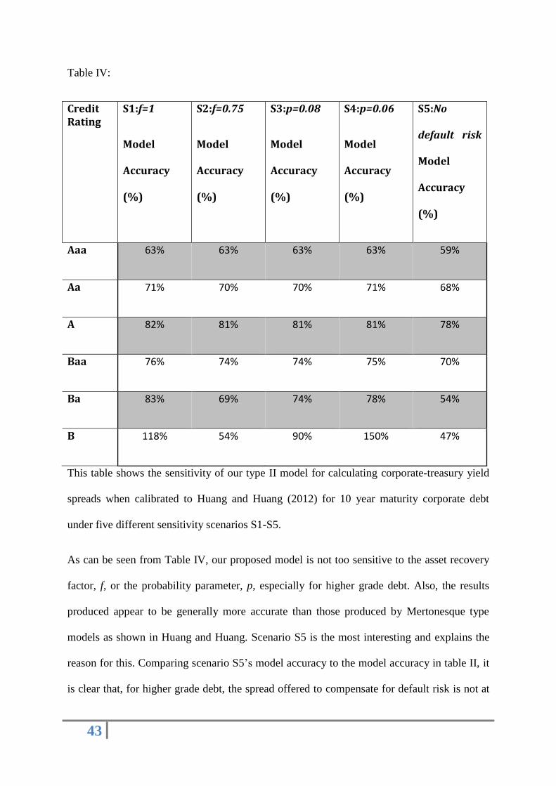
As can be seen, the proposed model appears to explain the credit premium puzzle reasonably

well. We now perform sensitivity analysis on the 10 year maturity results by varying the

model parameters. In our sensitivity analysis, we hold all the model parameters the same (in

Table I and Table II above) except for the one parameter on which sensitivity analysis is

being performed. We consider five scenarios. In scenario S1, we choose the asset recovery

factor, f=1. In scenario S2, we choose the asset recovery factor, f=0.75. In scenario S3, we

set p=0.08, for all six grades of debt. In scenario S4, we set p=0.06, for all six grades of debt.

In other words, in scenarios 3 and 4, we simply discard the information contained within the

Equity Risk Premium as given by Huang and Huang. In scenario S5, we perform the unusual

but interesting test of assuming that corporate bond holders of all six grades of debt are

offered zero spread for default risk but are allowed to share in the spoils of the tax

deductibility of interest in the manner described in section 3.4. We perform this feat by

setting the risk neutral rate covering default risk to be equal to the risk free rate, y*=rN in

equation 19. Table IV presents the results of the sensitivity analysis for scenarios 1-5.

43

Table IV:

Credit Rating

S1:f=1

Model

Accuracy

(%)

S2:f=0.75

Model

Accuracy

(%)

S3:p=0.08

Model

Accuracy

(%)

S4:p=0.06

Model

Accuracy

(%)

S5:No

default risk

Model

Accuracy

(%)

Aaa 63% 63% 63% 63% 59%

Aa 71% 70% 70% 71% 68%

A 82% 81% 81% 81% 78%

Baa 76% 74% 74% 75% 70%

Ba 83% 69% 74% 78% 54%

B 118% 54% 90% 150% 47%

This table shows the sensitivity of our type II model for calculating corporate-treasury yield

spreads when calibrated to Huang and Huang (2012) for 10 year maturity corporate debt

under five different sensitivity scenarios S1-S5.

As can be seen from Table IV, our proposed model is not too sensitive to the asset recovery

factor, f, or the probability parameter, p, especially for higher grade debt. Also, the results

produced appear to be generally more accurate than those produced by Mertonesque type

models as shown in Huang and Huang. Scenario S5 is the most interesting and explains the

reason for this. Comparing scenario S5’s model accuracy to the model accuracy in table II, it

is clear that, for higher grade debt, the spread offered to compensate for default risk is not at

44

all the key driver of corporate–treasury yield spreads. In fact, it is the sharing of the spoils of

the tax deductibility of the interest coupon that is the key driver of corporate-treasury yield

spreads for higher grade debt. For lower grade debt, both default risk and the sharing of tax

deductibility of interest coupons become important.

Discussion

Competitive Advantage is an important and well-worn subject matter in business schools

around the world. It is also strongly advocated by successful investors like Warren Buffett.

However, modern finance theory gives only cursory acknowledgement to competitive

advantage. In a recent paper, Rajaratnam et al (2014) show how one may incorporate

Competitive Advantage into equity valuation. In this paper, we tackle the important topic of

term structure of corporate credit and analytically show how term structure is influenced by

the competitive advantage of the firm. To the best of our knowledge, this is the first time a

formal link has been established between a firm’s competitive advantage and the term

structure of its debt, although, it is rather intuitive that these two factors are related. We

demonstrate in this paper that our proposed approximate model overcomes some of the well-

known shortcomings of structural form models (such as complexity, limited tractability and

the under-prediction of credit spreads).

Appendix A

Assuming b is constant, consider the following helpful identities derived by manipulating the

standard identity for finite and infinite geometric series:

Identity A1: for 0≤p≤1, r≥0

∑ 𝑏(1−𝑝)𝑖

(1+𝑟)𝑖+1𝑁−1𝑖=0 =

𝑏

𝑟+𝑝(1 −

(1−𝑝)𝑁

(1+𝑟)𝑁) (𝐴. 1)

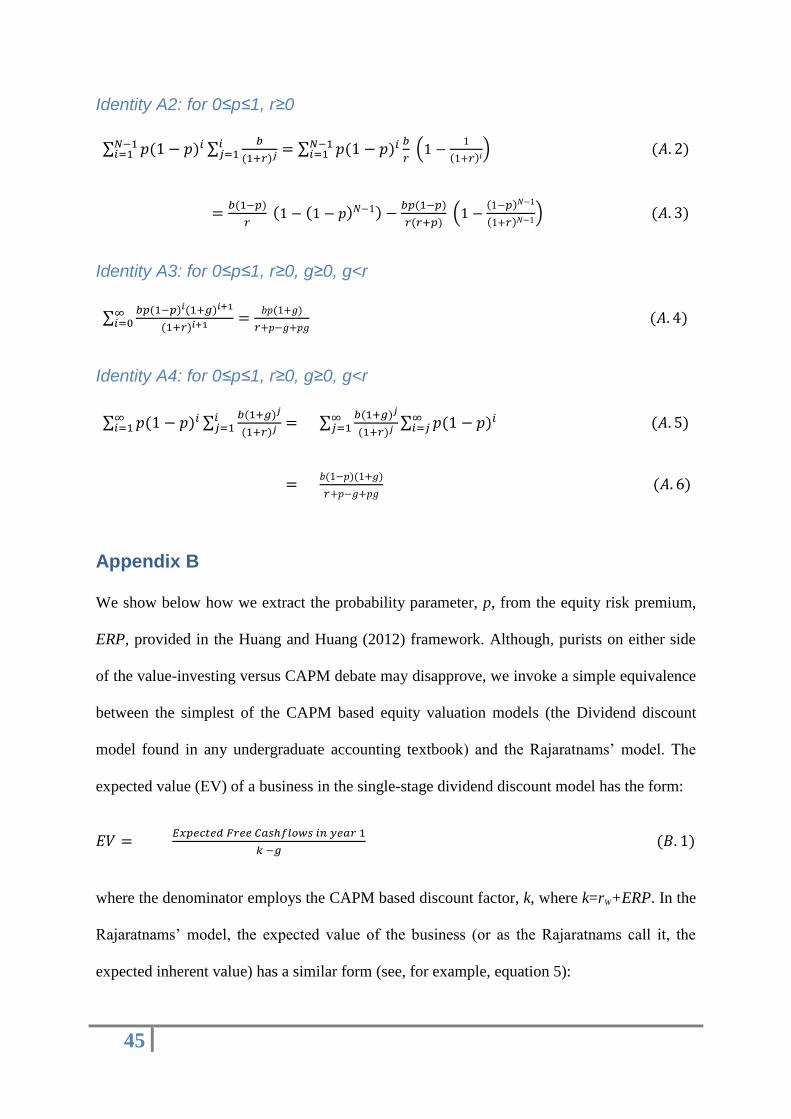
45

Identity A2: for 0≤p≤1, r≥0

∑ 𝑝(1 − 𝑝)𝑖 ∑𝑏

(1+𝑟)𝑗𝑖𝑗=1

𝑁−1𝑖=1 = ∑ 𝑝(1 − 𝑝)𝑖 𝑏

𝑟 (1 −

1

(1+𝑟)𝑖)𝑁−1

𝑖=1 (𝐴. 2)

=𝑏(1−𝑝)

𝑟 (1 − (1 − 𝑝)𝑁−1) −

𝑏𝑝(1−𝑝)

𝑟(𝑟+𝑝) (1 −

(1−𝑝)𝑁−1

(1+𝑟)𝑁−1) (𝐴. 3)

Identity A3: for 0≤p≤1, r≥0, g≥0, g<r

∑𝑏𝑝(1−𝑝)𝑖(1+𝑔)𝑖+1

(1+𝑟)𝑖+1∞𝑖=0 =

𝑏𝑝(1+𝑔)

𝑟+𝑝−𝑔+𝑝𝑔 (𝐴. 4)

Identity A4: for 0≤p≤1, r≥0, g≥0, g<r

∑ 𝑝(1 − 𝑝)𝑖 ∑𝑏(1+𝑔)𝑗

(1+𝑟)𝑗𝑖𝑗=1

∞𝑖=1 = ∑

𝑏(1+𝑔)𝑗

(1+𝑟)𝑗∑ 𝑝(1 − 𝑝)𝑖∞

𝑖=𝑗∞𝑗=1 (𝐴. 5)

= 𝑏(1−𝑝)(1+𝑔)

𝑟+𝑝−𝑔+𝑝𝑔 (𝐴. 6)

Appendix B

We show below how we extract the probability parameter, p, from the equity risk premium,

ERP, provided in the Huang and Huang (2012) framework. Although, purists on either side

of the value-investing versus CAPM debate may disapprove, we invoke a simple equivalence

between the simplest of the CAPM based equity valuation models (the Dividend discount

model found in any undergraduate accounting textbook) and the Rajaratnams’ model. The

expected value (EV) of a business in the single-stage dividend discount model has the form:

𝐸𝑉 = 𝐸𝑥𝑝𝑒𝑐𝑡𝑒𝑑 𝐹𝑟𝑒𝑒 𝐶𝑎𝑠ℎ𝑓𝑙𝑜𝑤𝑠 𝑖𝑛 𝑦𝑒𝑎𝑟 1

𝑘 −𝑔 (𝐵. 1)

where the denominator employs the CAPM based discount factor, k, where k=rW+ERP. In the

Rajaratnams’ model, the expected value of the business (or as the Rajaratnams call it, the

expected inherent value) has a similar form (see, for example, equation 5):

46

𝐸𝑉 = 𝐸𝑥𝑝𝑒𝑐𝑡𝑒𝑑 𝐹𝑟𝑒𝑒 𝐶𝑎𝑠ℎ𝑓𝑙𝑜𝑤𝑠 𝑖𝑛 𝑦𝑒𝑎𝑟 1

𝑟𝑊+𝑝 −𝑔+𝑝𝑔 (𝐵. 2)

Thereafter, by invoking equivalence between the two models, we can set the two

denominators in the above two equations to be the same and obtain p = ERP/(1+g).

References

Akerlof, G.A., Shiller, R.J., 2009. Animal Spirits. New Jersey: Princeton University Press.

Black, F., and Scholes, M., 1973. The pricing of options and corporate liabilities, Journal of

Political Economy, 81: 637-654, May-June 1973.

Buffett, W.E., 1977-present. Chairman’s letter to shareholders of Berkshire Hathaway inc.,

Available on www.berkshirehathaway.com.

Elton, E.J., Gruber, M.J., Agrawal, D., Mann, C., 2001. Explaining the rate spread on

Corporate Bonds. Journal of Finance, 56: 247-277, February 2001.

Huang, J.Z., Huang, M., 2012. How much of the Corporate-Treasury Yield spread is due to

credit risk? Review of Asset Pricing Studies, 2:153-202.

Kelly, J.L., 1956, A new interpretation of the information Rate. Bell System Technical

Journal, 35, pp. 917-926.

Lintner, J., 1965. The valuation of risk assets and the selection of risky investments in stock

portfolios and capital budgets. Review of Economics and Statistics, 47(1), 13-37.

MacLean, L.C., Thorp, E.O., Ziemba, W.T., (Eds.), 2011. The Kelly Capital Growth

Investment Criterion: Theory and Practice. World Scientific Press, Singapore.

Markowitz, H., 1952. Portfolio selection. Journal of Finance. 7:1, pp. 77-99.

Merton, R., 1974. On the pricing of Corporate Debt: The risk structure of interest rates.

Journal of Finance, 29, 449-469

47

Modigliani, F., and Miller, M., 1958. The cost of capital, corporation finance, and the theory

of investment. American Economic Review, 48, 267-297.

Porter, M., 1980. Competitive Strategy, Free Press, New York.

Rajaratnam, M., Rajaratnam, B., Rajaratnam, K., 2014. A novel equity valuation and capital

allocation model for use by long-term value-investors. Accepted for publication in the

Journal of Banking and Finance. DOI: 10.1016/j.jbankfin.2014.02.014 Available online

Feb 2014: http://www.sciencedirect.com/science/article/pii/S0378426614000776

Samuelson, P., 1971. The fallacy of maximizing the geometric mean in long sequences of

investing or gambling. Proceedings National Academy of Science 68, pp. 2493-2496

Schumpeter, J., 1942. Capitalism, Freedom and Democracy. New York: Harper and Bros.

Sharpe, W.F., 1964. Capital asset prices: a theory of market equilibrium under conditions of

risk. Journal of Finance, 14(3), 425-441.

Shleifer, A., 2000. Inefficient Markets: An Introduction to Behavioral Finance. Oxford

University Press.

Thaler, R., 1993. Advances in Behavioral Finance, New York, Russell Sage Foundation.

Thorp, E.O., 2010. Understanding the Kelly criterion and other articles by E.O. Thorp. In:

MacLean, L.C., Thorp, E.O., Ziemba, W.T., (Eds.), The Kelly Capital Growth Investment

Criterion: Theory and Practice. World Scientific Press, Singapore.

Tversky, A., Kahneman, D., 1974. Judgment under uncertainty: heuristics and biases. Science

185 (4157), 1124-1131.