Munich Personal RePEc Archive

A systematic review of statistical

methods for estimating an education

production function

Ogundari, Kolawole

12 January 2021

Online at https://mpra.ub.uni-muenchen.de/105283/

MPRA Paper No. 105283, posted 15 Jan 2021 01:31 UTC

1

A systematic review of statistical methods for estimating an education production function

Kolawole Ogundari

Education Research and Data Center

Olympia, Washington State USA

Email: ogundarikolawole@daad-alumni.de

Abstract

The quality of administrative or longitudinal data used in education research has always been an

issue of concern since they are collected mainly for recording and reporting, rather than research.

The advancement in computational techniques in statistics could help researchers navigates many

of these concerns by identifying the statistical model that best fits this type of data for research.

The paper provides a comprehensive review of the statistical methods important for estimating

education production function to recognize this. The article also provides an extensive overview

of empirical studies that used the techniques identified. We believe a systematic review of this

nature provides an excellent resource for researchers and academicians in identifying critical

statistical methods relevant to educational studies.

Keywords: Education, Production Function, Statistical Methods, Causal Analysis, Regression

Introduction

A production function is defined as a technical relationship between input and output. The concept

of production function has been applied widely to the different sectors of the economy, such as

agriculture, energy and power, transportation, finance, education, and the healthcare sector, among

others (see: Clark 1984; Just et al., 1983; Boyd 2008; Sami et al., 2013; Koc 2004; Gyimah-

Brempong and Gyapong 1991). In the education sector, the production function is considered a

powerful tool to understand the combination of school inputs that influence education outcomes

(Espinosa 2017). Here the educational institution is analogous to transforming inputs into outputs

through a production process (Worthington 2001). Unlike other industries, schools are treated

2

analytically as production units on the supply side when estimating education production function.

With few exceptions, schools are not considered profit-maximizing firms, especially the public or

private non-profit ones.

According to Worthington (2001), the output in education production function may either

be defined in terms of intermediate outcomes such as student test score (e.g., math or reading test

scores, CGPA, number of pupils, number of graduates, and passing rates, etc.) or education

outcomes (e.g., employment rates, starting salaries or acceptance rates into higher education). The

author also noted that the typical inputs in education production function are the teaching and

learning environment's characteristics. This comprises students' attendance and homework;

expenditure on education; technology (equipment); teachers' experience, certification, salary;

pupils/teacher ratio; class size; and parents' education and income levels.1, 2

The estimation of education production function provides mechanisms through which

researchers can understand productivity in schools or educational institutions described as

improving student outcomes with little or no additional resources (Hanushek, 1979). This explains

why education production function's policy relevance has long been stressed in the literature (Todd

and Wolpin, 2006; Hanushek, 2007). Unfortunately, the quality of administrative or longitudinal

data used in education research has always been an issue of concern since they are collected mainly

to record and report or provide necessary information about service users, rather than research.

The advancement in computational techniques in inferential statistics has helped researchers

identify the statistical methods that best fit their data over the years. This has led to a shift in the

empirical strategies among the researchers. For example, there is an increasing move from simple

multivariate statistical methods to more sophisticated techniques such as Bayesian, non-parametric

regression, semiparametric regression, and machine learning applications, among others, in recent

years. In contrast to other economic sectors, such as energy and power, transportation, finance,

health, and agriculture, some of these methods are scarce in education research.

1 The choices of output and input measures are driven by data availability. 2 Although the purported relationship between key policy variables such as resource spending or educational

expenditure and educational outcomes has been the subject of much inquiry (Hanushek, 1986), the quality of many of

these measures is another concern when estimating education production function (Grosskopf et al., 2014). Most

economists prefer the value-added measure that requires access to panel data on individual students to mitigate the

quality problem in the education production function (Gronberg et al., 2011). None of these is the focus of this paper.

3

The application of statistical techniques that best fit an education data provides

opportunities for researchers to accurately understand the dynamic relationship between education

outcomes and associated factors such as students, schools, parents, and teachers' characteristics.

Of course, determining appropriate statistical methods matter, as this validates estimated results

for policy. Inferential statistical methods such as regression have always been used to fit education

data. According to Hanushek (1997), regressions use a series of independent or descriptor variables

to estimate the value of the dependent or, in this case, the outcome variable. Example of regression

used in education research includes parametric regression models such as ordinary least square -

OLS, logistic regression, probit regression, multinomial regression, Tobit regression, fixed effect

regression, mixed model, random effect regression and generalized method of moment regression,

etc. Others include non-parametric regression, such as kernel regression and semi-parametric

regression.

Based on a systematic review of prior research works and literature, we observed that

education research questions have always been framed in two ways highlighted below.

1. What are the effects of students, schools, or teacher characteristics on education outcomes?

2. What is the impact of educational programs or policies on education outcomes?

The education production function is often used as the conceptual framework to address

these questions in the literature empirically (Worthington, 2001). For example, education

production function specified to link resource inputs (e.g., pupil to teacher ratios, technology,

amount of homework, teacher experience, teacher education, teacher salary, school expenditure,

teacher/pupil ratios, class size, etc.) with educational outcomes (e.g., reading and math test score,

CGPA, SAT, etc.) after controlling for student, parent, teacher, and school characteristics (e.g.,

student gender, age, and ethnicity, student attendance, teacher certification, etc.) is synonymous to

the first question. This includes estimating schools' relative efficiency, among others (see;

Scippacercola and Ambra, 2013; Halkiotis et al., 2018). Also, education production function

specified to link treatment assignment ( e.g., STEM program, remedial program, honor program,

or early learning education, etc.) with educational outcomes (e.g., reading and math test score,

CGPA, SAT, etc.) after controlling for student, parent, teacher, and school characteristics (e.g.,

student gender, age, and ethnicity, etc.; parent education; teacher salary and experience, etc.) is

4

synonymous to the second question. This includes estimating the impact of early learning

program/preschool on educational outcome among others (see; Hogrebe and Strietholt 2016;

Atteberry et al., 2019)

In recognition of this, the objective of this paper is two-fold. First, to identify the best

statistical methods for estimating education production function that aligns with each of the

research questions above. Second, to provide a detailed example of the studies that used the

statistical methods identified within the context of education data.

The paper is structured as follows. Section 2 provides essential guidelines for selecting

statistical methods within the context of education data given the data generating process (DGP).

Sections 3 and 4 identify statistical methods for estimating the education production function that

aligns with the first and second research questions. While section 5 describes the available

statistical software for analyzing the statistical techniques identified in the paper, section 6

concludes.

2.0. Essential guidelines for selecting statistical methods in education research

Quantitative researchers seek to identify the statistical methods that best fit their studies'

data. Understanding the data generating process (DGP) is crucial to achieving this, most

importantly, the dependent variable. The model's selection depends on the outcome or dependent

variable (Osgood, 2008). For instance, it is vital to address the following questions: How is the

dependent variable measured or constructed in the data? Is the dependent variable continuous or

discrete? If the dependent variable is discrete, is it a binary, ordinal, categorical, proportional,

percentage, or count variable?

Osgood (2008) noted that despite the ordinary least square (OLS) violation of fundamental

general linear model assumptions, the model is still used in educational research for count

dependent variables. Liou (2009) also revealed that the statistical analysis's conclusions might

influence their estimated standard errors and inferential statistics and invalidate the results due to

errors in selecting the appropriate regression model. For example, a review of the literature shows

that Ayalon and Yogev (1997) used hierarchical linear modeling to estimate the relationship

between students’ characteristics and the types of courses that science and humanity students take.

They also explore the effects of school characteristics on these relationships. At the student level,

5

the dependent variable was the number of course units’ students in science or humanities take in

the study. Unfortunately, the authors employed a hierarchical linear model instead of a hierarchical

count model (e.g., multilevel mixed-effects Poisson regression model). This is because the DGP

of the dependent variable has a characteristic of count data. Hence, using a hierarchical linear

model rather than a hierarchical count model may influence estimated standard errors and

invalidate the results.

Another important concern is the case of missing data. This is a common phenomenon in

administrative or longitudinal data. Thus, quantitative researchers must understand the nature of

the missing data, which could help identify statistical methods that best fit the data. For example,

it is important to note the missing cases could be random or non-random. If the missing is random,

one could impute the missing cases using appropriate imputation methods available in the

literature. However, if the missing cases are nonrandom, it cannot be imputed. The issue of

nonrandom missing cases must be put into consideration when estimating the model. For instance,

in the case of dependent variables with missing cases at nonrandom, the researchers must address

the following questions. Is the dependent variable censored, truncated, or is it a corner solution or

a problem of sample selection bias? Understanding the theoretical or empirical processes that

create the zeros helps identify the appropriate model that best fits the data.

3.0 Methods for addressing the first research question

As earlier mentioned, an education production function can be specified to study the effects of

students, schools, or teacher characteristics on education outcomes. The subsequent sub-sections

describe inferential statistical methods that best fit the dependent variables of different forms often

used to address this type's research question.

3.1.0 A regression model with cross-sectional data

A regression model is the most popular inferential statistic method used in applied research to

answer research questions. While there are several types of regression models, identifying the

appropriate regression model that best fits the data has enormous implications on the policy's

validity.

6

3.1.1 Linear Ordinary Least Square (OLS) regression model

The ordinary least square (OLS) regression model is prevalent in applied research. It is important

to note that OLS is considered an unbiased estimator of a linear regression model (specification

similar to equation 1 in the Appendix) with a continuous dependent variable. The dependent

variable's precise nature is continuous, which is very important when selecting OLS as an

estimator. However, OLS maintains stringent assumption of a normal distribution of error terms

and linear functional relationship between dependent and explanatory variables.

Kruger (1997) employed OLS to estimate an education production function to explore the

effects of class-size assignments on the average percentile of standard achievement tests for

kindergarten through third grade. This study's dependent variable is the standardized test score, a

continuous variable. Fuller and Ladd (2013) used OLS to examine teacher quality's effects on

students’ scores. The student test score in this study is also a continuous variable. Other examples

include Chakraborty and Jayaranman (2019) that employed the OLS regression model to explore

the school feeding program's effect on children learning outcomes.

3.1.2. Tobit, Heckman, and Double hurdle regression models

The analytical method changes when the dependent is not continuous as described in the

previous section but appears to be discrete such as censored or truncated at a point, exhibit corner

solution, or sample selection bias problem with positive and zeros outcome due to missing data.

Here, the dependent variable is assumed to follow a mixed distribution where there is a probability

mass at zero and a continuous distribution for values greater than zero (Amore and Murtinu 2018).

Tobit, Heckman, truncated, or Double hurdle regression is a particular case of models with a

limited dependent variable. In this case, the zeros due to missing data cannot be imputed because

they are assumed to not missing randomly. When the dependent variable is configured this way,

OLS is considered biased (Maddala 1983). Thus, ignoring censoring or sample selection bias in

OLS translates into a lower regression line slope and an inflated intercept. Tobit models, Heckman

selection models, and the Double hurdle regression model may constitute a valid estimation

approach depending on a clear understanding of the source of zeros or missing patterns in the data

(see; Tobin, 1958; Heckman, 1979; Cragg 1971).

7

Tobit models’ assumption of zero observations in a limited dependent variable is due to

censoring attributed to the corner solution problem, where zeros are considered true or genuine

zeros. Data censoring in Tobit usually arises from data observability and should not be associated

with sample selection bias (Amore and Murtinu 2019). Tobit model is traditionally referred to as

censored regression (Wooldridge 2010).

Heckman's sample selection model (see Heckman, 1979) and the double hurdle model (see

Cragg 1971) are a generalization of the type 1 Tobit model (see Tobin, 1958). Heckman's model

assumes zero observation is due to sampling selection bias rather than a corner solution problem.

Here, zeros due to missing data are referred to as false zeros because it comes from a separate

discrete decision rather than a corner solution as in the Tobit model. As a result, the Heckman

model assumes two distinct outcomes that govern positive and zero observations. The first

represents a selection equation that describes the probability of a non-zero (e.g., equation 4 in the

Appendix). The second is the outcome equation that defines a positive observation (e.g., equation

3 in the Appendix). If the two equations are independent, the model reduces to the Tobit model.

The implication of this is that selection decisions influence the actual outcome (i.e., the positive

values) do not hold. As Heckman (1979) proposed, the first stage involves estimating the selection

equation of probability of treatment similar to equation 4 of the Appendix to derive a bias

correction variable in the form of inverse mills ratio (IMR). The second stage is the outcome

equation (e.g., equation 3 of the Appendix), where the IMR is part of the explanatory variables.

An example of this is a study of the effect of education on earnings only on data for public sector

workers. Sample selection bias arises because zeros are associated with a focus on public sector

workers.

On the other hand, the double hurdle model allows for censoring due to the corner solution

as a zero observations source. Nevertheless, zeros here have features of true and false zeros.

However, the model assumes that two hurdles governed positive and zero observations. The first

and second hurdles are sequential or simultaneous. The first hurdle deals with the binary decision,

as the second hurdle deals with the positive outcome (e.g., equation 4 of the Appendix).

Technically speaking, the first hurdle corresponds to the probability of non-zero observation, and

the second hurdle corresponds to the level of positive observation (e.g., equation 7 of the

8

Appendix). Residuals of the first and second hurdles are correlated in the Double Hurdle model,

but the model reduces to the Truncated Hurdle model (see Cragg, 1971).

A study that examined the effects of educational qualification or certification on earnings

is a good example. Here, data on earnings has both positive and zero outcomes with the possibility

of corner solutions, censoring, or sample selection problem in the data. In this example, due to the

data provider's privacy concerns, earnings are not observed for the whole population (case of

censoring problem). It is also possible some of the data providers are unemployed during the

survey (selection bias problem). The nature of the dependent variable (earnings) shows that

researchers cannot simply delete observations with zero earnings as this bias results from the

policy. Likewise, selecting the ordinary least square (OLS) regression model is considered a biased

estimator for this type of dependent variable. Double Hurdle, Tobit, Heckman, or sample selection

models are possible methods of estimating such data, depending on a clear understanding of the

data generating process (DGP).

Ogundari and Aromolaran (2014) employed a double hurdle model to examine the effect

of educational attainment on earnings in Nigeria. The income column has zero due to missing data

for many of its data observations in the study. The authors assume two hurdles govern the zeros

and non-zeros income with the possibility of zeros associated with true or false zeros in the study.

Tsai and Xie (2011) used the Heckman selection model to model heterogeneity in college

education returns in contemporary Taiwan. The data on earnings has zeros due to missing data,

which the authors assume is due to sampling selection bias. The authors estimate a first-stage

probit model for selection into labor force participation to derive inverse mills ration (IMR), which

is then included in earnings function as an explanatory variable to correct selection bias.

3.1.3. Univariate Probit and Logit regression models

Univariate probit and logit regression models are models with the categorical dependent

variables and are classic examples of regression models with the limited dependent variable. The

dependent variable here is a dichotomy or binary response. An example of this is the participation

in a STEM program or early learning program where participation is a binary response recorded

in the data as 1 and 0 otherwise. The difference between the logit and probit model is the error

terms' underlying distribution. Probit has a cumulative standard normal distribution, while logit

uses cumulative standard logistic distribution. The two models produce similar results. OLS

9

application to a binary response-dependent variable may lead to predictions outside the range of 0

and 1, and the residuals are also heteroskedastic by construction.

Pyke and Sheridan (1993) employed logistic regression to analyze graduate student

retention, where the dichotomous dependent variable was whether the student completed masters

and Ph.D. degrees. Bautsch (2014) used a logistic regression model to explore the effects of

concurrent enrollment in college-going and remedial education rates of Colorado’s High School

students. This study's dependent variable is binary such that college enrollment or remedial is taken

as 1 and 0 otherwise.

3.1.4. Ordered and multinomial regression models

Other limited dependent variable models of interest include the ordered and multinomial

models. Ordered and multinomial models are two extensions of binary dependent models referred

to as categorical models. However, the difference between these two models is how the dependent

variable is structured as categorical data. The dependent variable in ordered response models takes

several finite and discrete values that contain ordinal categorical data. Examples of these ordered

models are the ordered probit and the ordered logit model. However, the multinomial model's

dependent variable takes finite and discrete values but does not have any ordinal information. The

two standard models are the multinomial probit and multinomial logit model.

Alauddin and Tisdell (2006) employed ordered probit to examine students’ evaluation of

teaching effectiveness with ordinal dependent variable ranging from 1 to 5. In their specification,

1 represents very poor, 2 for poor, 3 for good, 4 for very good, and 5 for outstanding, defining the

ordinal dependent variable in the study. Stratton et al. (2005) employed a multinomial logit model

to examine college stop out and dropout behavior. This study's dependent variable is a non-ordinal

variable where continuous enrollment is recorded as 1, stop out as 2, and dropout as 3. Nguyen

and Taylor (2003) also used a multinomial logit model to examine post-high school choice

determinants. In this study, 1 to 5 represent the private four-year college, public four years, private

two-year college, public two-year college, and employed, respectively, as the study's dependent

variable.

10

3.1.5. Multivariate binary models

A typical example of this is a multivariate probit model, a generalization of the probit

model discussed above and estimates several correlated binary outcomes jointly. For example, a

bivariate probit regression model estimates two binary dependent outcomes believed to be

correlated. A multivariate probit model can accommodate more than two dependent outcomes as

an interdependent binary response. Even when the binary dependent outcomes are more than two,

the joint prediction can be carried out individually.3

Using the data from South Africa, Chisadza (2015) employed a bivariate probit model to

model the joint probability of school enrollment and work-study on the transition from school to

work in the post-compulsory schooling period. In this example, the dependent variable is

“enrollment” and “working.” The methodology is best appropriate given that there is a likelihood

of having an individual working and, at the same time, enrolled in school in the dataset. Also, there

might be individuals that are only working and not enroll in school and vice versa in the dataset.

Evans and Roberts (1995) jointly modeled the probability of being a member of the catholic church

and attending a Catholic school in a study to examine the effect of catholic secondary schooling

on educational attainment. In this study, there is a high likelihood that the catholic church members

are more likely to attend catholic schools and should be modeled accordingly. There is also the

possibility of having an individual who attends a catholic school but not a catholic church member

and vice versa. Bowles and Jones (2004) employed the bivariate model to jointly model the

probability of supplemental instruction and retention in a study that examined the effect of

supplemental instruction on retention.

3.1.6. Non-parametric Regression model

A parametric model such as ordinary least square (OLS) and generalized linear model (GLM) has

a strong assumption regarding a definite functional form concerning a subset of the regressors or

the density of the errors that are assumed to be normally distributed. Taking a specific distribution

of the error term beforehand might not work with most data given the data generating process

3 It is important to note that the interdependence of binary response in the multivariate setting should be taken into

account during estimation. In the absence of interdependence, the model collapses to a univariate binary response

model.

11

(DGP). Fan and Yao (2003) noted that when a wrong functional form is selected, the results are

substantially biased compared to the other competitive models. Unlike OLS, non-parametric does

not maintain the stringent prior assumption of a specific distribution of error terms and functional

form relationships between the dependent and explanatory variables. In non-parametric

regression, the appropriate model is determined from the data set and can take any shape, which

could be linear or nonlinear.

Non-parametric regression models such as kernel smoothing regression, locally weighted

scatterplot smoothing (LOWESS), Local regression (LESS), and Robust weighted local regression

relaxed the stringent assumptions of the parametric models. The models are executed as a graph

and are a valuable method in visualizing the relationship between education outcomes such as

earnings and factors and conditions associated with it, such as educational level and experience.

For example, nonparametric regression gives you a visual insight into the pattern of the

relationship between earnings and education attained, which could be linear or non-linear.

A literature review shows that the non-parametric regression model is not widely used in

education research. However, we believe non-parametric regression could prove useful when

examining the relationship between educational outcomes such as academic performance (e.g.,

test score and CGPA) and factors such as attendance and teacher experience, and salary, among

others. It is important to note that both the education outcomes and the factors of interests are

assumed to be a continuous variable when using non-parametric regression.

3.1.7. Semi-parametric regression model

The semi-parametric regression model combines the features of parametric and non-parametric

models. This model has a parametric component) and an indefinite dimensional nuisance

parameter (the nonparametric component). It is useful when fully, nonparametric models may not

perform well or when the researcher wants to use a parametric model when the functional form of

the regressors or the errors' density is unknown. This model includes regression splines, fractional

polynomial regression model, and the Cox proportional hazards model.

Goldhaber et al. (2007) employed a semi-parametric model to assess teachers' career

transitions and their implications for the teacher workforce quality in North Carolina public

schools from 1996 to 2002. Likewise, Feng and Sass (2011) used the Cox proportional hazards

12

model to study the relationship between teacher productivity and inter-school mobility. The

students' demographic and economic backgrounds are included in the estimated hazard model.

3..1.8. Other regression models/approaches

a. A regression model with count dependent data

The regression model for count data is an important model for investigating the relationship

between factors and conditions associated with educational outcomes. While the regression model

is an extension of GLM, OLS is considered unsuitable for analyzing discrete count data (Cameron

and Trivedi 1998). The regression models used for handling count data include a zero-truncated

Poisson regression model, zero-truncated negative binomial, zero-inflated Poisson, random effects

count models, and Poisson regression.

Desjardins (2015) employed four models: Poisson, negative binomial, Poisson hurdle, and

negative binomial hurdle to explain variability in school days suspended. The number of school

days suspended is a count dependent variable in the study. Eminita and Widiyasari (2019)

employed Poisson and Binomial Negative Regression models to examine the factors affecting

undergraduate students' quitting in their research. The authors used the number of courses that

students failed in the semester as the dependent variable. Salehi and Roudbari (2015) employed

Zero-inflated Poisson and negative binomial regression models to explore factors associated with

students’ failure.

b. Multilevel regression model

A multilevel regression model is an extension of the Generalized linear model (GLM)-a flexible

generalization of the ordinary linear regression of OLS that allows for response variables with

error distribution models other than a normal distribution. The multilevel regression model is also

referred to as a Hierarchical linear model (HLM) or mixed level models. When observations on

students are not entirely independent but rather clustered in the district, school, year, zip code, or

other factors, simple regression such as OLS is often not the best strategy (Theobold 2018). OLS

is biased because students within a cluster (e.g., schools or districts) share experiences that are not

shared across the schools or districts in the data, as observations in the same cluster are most likely

correlated.

13

One-way to account for this type of clustering or dependence is by fitting multilevel

regression models that include both fixed effects (e.g., explanatory variables) and random effects

(variables by which students are clustered such as schools, years, districts, etc.) components.

Multilevel regression controls for non-independence of sampling due to variations at multiple

levels with fixed effects and random effects components in the model. Pedhazur (1997) noted that

a multilevel regression model or HLM estimates variance between groups as distinct from variance

within groups. Thus, it solves aggregation bias problems and misestimated standard errors and

heterogeneity of regression. It is necessary to note that multilevel regression modeling does not

correct the regression coefficient estimates' bias than an OLS model. However, it produces

unbiased estimates of the standard errors associated with the regression coefficients when the data

are nested and easily allows group characteristics to be included in individual outcomes models

(O’Dweyer et al., 2014).

Lee (2000) employed HLM to study school effects and social contexts on students’

academic development. Munoz et al. (2011) also used HLM to explore teacher effectiveness on

student performance denoted by reading test. Parker et al. (2014) employed a multilevel regression

model to investigate the effects of students’ and school characteristics on a test of English

proficiency. The authors clustered the data across the school level. This methodology is prevalent

in education research because students' observations are clustered in schools, districts, zip codes,

and administrative data years. A detailed discussion of this model in education research can be

found in Theobald (2018) and O’Dweyer et al. (2014).

Besides the continuous dependent variable, the multilevel regression model or HLM has

been extended to other dependent variables with a binary outcome such as probit and logit

regression models, Poisson regression model for count data, ordered logit/probit model, and

proportional or fractional regression model among others.

c. Structural Equation Model (SEM)

SEM is a comprehensive and flexible statistical technique for analyzing the structural relationship

between measured variables and latent constructs with multiple pathways. It combines factor

analysis and multivariate regression analysis to estimate interrelations between outcome variables

(Kline 2011) simultaneously. Of course, this allows researchers to analyze multiple associates

between outcomes and related inputs. SEM consist of two components: measurement model and

14

structural model. The former deals with the relationship between the observed indicator variables

and the latent variables/factors. The latter deals with the various relationships among latent

variables based on theoretical frameworks. A common SEM application practice is constructing a

diagram or path diagram for model specification. Each latent variable is defined with its observed

indicators variables and the relationship between variables, including latent and observed

variables. 4

A review of the literature shows that McKeon et al. (2015) employed SEM to assess the

determinants of child outcomes in a cohort of children in the free pre-school year in Ireland.

Espinosa (2017) used SEM to investigate the relationship between child, school, and teacher

characteristics and educational outcomes related to cognitive and non-cognitive skills. Rashkind

et al. (2019) employed SEM to examine whether test psychosocial health mediates the association

between food insecurity and academic performance. GPA is the measure of academic performance

in the study.

d. Latent Class Analysis (LCA)

The latent class analysis (LCA) is a latent class modeling approach used to estimate the subject's

latent class probabilities belonging to any classes ( or groups). This is subsequently related to the

covariates and distant outcomes, mostly when latent classes (a group of respondents) are assumed

to exist in data. Collins and Lanza (2010) described LCA as a modeling approach used to classify

respondents' groups similar to some unobserved construct based on their observed response

patterns. In this case, the conditional probability that potential outcomes reflect subgroups of cases

in multivariate data. In LCA, group membership is not known or observed in the data but instead

assumed to be unobserved (latent) while identifying groups of individuals who share common

attributes. However, the dependent variable's underlying construct is a categorical outcome that is

not observed ( or known beforehand) but with different ways to evaluate the probability of subject

belonging to particular outcome groups.

A review of the literature shows that Bowers and Sprott (2012) employed LCA to examine

a typology of high school dropouts (i.e., Jaded, Quiet, and involved) as the latent classes considered

in the study. Weerts et al. (2013) employed LCA to identify four student groups to estimate latent

4 The application of SEM in education research can be found in Wang et al. (2017).

15

class probabilities (i.e., super engagers, social-cultural engagers, Apolitical Engagers, and Non-

Engagers) in the study. Denson and Ing (2014) employed LCA to classify students into latent

groups on their pluralistic orientation at the start of college, with five classes identified in the study.

Each study examines whether latent classes identified relate to the respondent’s demographic and

background characteristics. Depending on the data generating process (DGP), LCA has always

been estimated using logistic regression when two classes are identified or multinomial logistic

regression when more than two categories are identified.

e. Bayesian Regression models (Parametric and nonparametric)

The standard regression models can provide misleading results because they make assumptions

that are often violated by real data sets or are not enough for dealing with noisy data. The traditional

regression model assumes that the error terms' distribution is independently and identically

distributed (IID) and assumed a specific functional form. The Bayesian models provide another

possible way to construct such a flexible model, defined by an infinite mixture of regression

models, that makes minimal assumptions about data. The Bayesian estimator used Markov Chain

Monte Carlo (MCMC) method for approximating prior distribution to generate posterior predictive

inference (Denison et al., 2002). The use of prior distribution to estimate a posterior distribution

is one of the most significant advantages of the Bayesian model, as it guaranteed coherent

inference.

The Bayesian regression model used prior probability distribution in suitable and plausible

probability distributions rather than point estimates to find the single best value of the model

parameters assumed to come from the same distribution. The necessary procedure for

implementing Bayesian Linear Regression is to specify priors for the model parameters ( e.g.,

normal distributions). Others include creating a model mapping the training inputs to the training

outputs and then have a Markov Chain Monte Carlo (MCMC) algorithm draw samples from the

posterior distribution for the model parameters. The result is the posterior distributions for the

estimated parameters.

The Bayesian regression model has been extended to the basic linear regression model and

nonlinear models. Besides the linear regression model, the Bayesian regression model has been

extended to binary regression (probit and logit), ordinal regression, and multilevel regression

model. The Bayesian regression model has been extended to censored regression, panel regression

16

model, and models used in the causal analysis, such as regression discontinuity design. There is

also a Bayesian nonparametric regression model.

The advantages of the Bayesian model include the ability to incorporate prior information.

It provides the entire posterior distribution of the model parameters and provides a more intuitive

interpretation of the results in terms of probabilities. The significant problem is that it is

computationally demanding.

Subbiah et al. (2011) noted that an appropriate method that could incorporate the subjective

nature of the available information in educational data would be an added advantage in dealing

with the uncertainties involved in these processes. Of course, this can be found in Bayesian through

a properly devised set of priors in the form of suitable and plausible probability distributions.

A review of the literature shows that Zwick (1993) employed the Bayesian regression

model to examine the degree to which GMAT scores and an undergraduate grade-point average

(UGPA) could predict first-year average and final grade point average in doctoral programs in

Business and management. Subbiah et al. (2011) employed the Bayesian regression model to

evaluate the effects of qualification mark, gender, and types of degree for which you are applying

(i.e., major in math, statistics, and other courses) on performance, which is represented by the

results of the entrance exam in India.

e. Machine learning regressions

Much has been written in recent times on applying machine learning tools in applied research,

given that ML has a better accurate predictive power than regular regression models (Athey and

Imbens, 2019). Despite this, a few studies have raised concerns about transparency,

interpretability, and identification of casual relationships in ML (Lazer et al., 2014). In contrast,

Storm et al. (2019) argue that ML offers excellent potential for expanding tools in applied research

or quantitative research in the long run.

Machine learning is a subfield of artificial intelligence that enables computers to use an

algorithm to find observed data patterns. The algorithm helps find the relationship of variables in

the existing data without pre-programmed rules. Therefore, the learned link is applied to classify

or predict with entirely new data using statistical methods (Kaliba et al., 2020). Using equation 1

of Appendix 3 as an illustration, supervised learning goals is to learn the relationship between the

17

dependent variable and independent variables. The learned relationship from the raw data then

predicts unknown values of a dependent as accurately as possible into distinct groups. In contrast

to econometric or statistical tools mentioned earlier (e.g., OLS, GMM, GLS, etc.), ML tools

manage to fit complex and very flexible functional forms to the data without overfitting

(Mullainathan and Spiess 2017).

Many machine learning tools are relevant in socio-science research, and many have already

used ML in applied research (see Kaliba et al., 2020; Liu et al., 2013). ML tools for predicting

models include shrinkage methods (ridge regression, least absolute shrinkage, and selection

operator (LASSO) regression); Tree-based methods (classification and regression trees-CART or

decision trees, random forests); Neural network (Neural convolutional network CNN, recurrent

Neural network RNN).

ML tools have also been extended to estimate causal inference besides ML tools as a

predictive model. As part of growing literature aiming at assessing heterogeneous causal effects

across observed covariates using ML, Athey, and Imbens (2016), Wager and Athey (2018), and

Lecher (2019) employed regression tree and random forest method. For example, Athey and

Imbens (2016) used recursive partitioning for heterogeneous causal effects based on the regression

tree method across subgroups defined upon the splits. The ML for causal inference has been

implemented in the R statistical software package “causalTree” by Athey et al. (2016). Surveys on

ML methods for assessing causal inference are available in Powers et al. (2018) and Knaus et al.

(2018).

However, a literature review shows that many studies have employed ML in education

research. Some of the ML tools used in education research include decision trees and random

forest, among others, to predict students’ performance or success and study the impact of effective

communication between students and teachers. They are also used as imputation methods for

education data in an attempt to gain further insights that could help shape policy recommendation

in the sector ( for detail see: Golino and Gomes, 2016; Shan et al., 2014; Al-Barrak and Al-Razgan,

2016; Topirceanu and Grosseck, 2017; McDaniel 2018). Greene (2019) employed CART to assess

differences between direct entry and transfer students and their progress towards a baccalaureate

degree in Washington.

18

3.2. Regression with a panel or longitudinal data

It is not clear how cross-sectional data based on a one-time measure of student outcomes and their

characteristics coupled with the teacher, school, and parent characteristics, will adequately provide

valuable student performance measures for effective policymaking. In contrast, longitudinal data

have clear analytical advantages over cross-sectional data because it allows for measurement of

change over time for robust and accurate inference for policymaking (Jyoti et al., 2005; Johnes et

al., 2017). Hsiao (2007) noted that regression with panel data produces a more accurate inference

of model parameters and a higher capacity to account for human behavior's complexity relative to

cross-section data. A model with panel data has two dimensions: time and individual-specific

effects. Panel data estimation is more complicated than cross-section data estimation (Hsiao 2007).

a. Linear Panel Data Model: Fixed and random effect regression models

The random-effect (RE) model and fixed-effect (FE) model (within estimator) are the most

common estimators applied to panel data. The fixed effect estimator assumes unobserved

heterogeneity to be arbitrarily correlated with time-varying explanatory variables. It also assumes

the covariates are strictly exogenous concerning the time-varying idiosyncratic errors. The fixed-

effects estimator transformed the model by fully demeaned (mean-centered) data to remove the

unobserved heterogeneity. The fixed effect estimator uses within-unit change and ignores

between-unit variation in this process. The fixed-effect estimator is called the within estimator in

this context. The unobserved heterogeneity can also be removed using the least square dummy

variable regression (LSDV) approach, where the time-invariant characteristic is treated as a fixed

parameter. With LSDV, a dummy variable is created for each sample unit and included as a

regressor in the model. The estimation is carried out using OLS.

The random effect assumes the explanatory variables are uncorrelated with unobserved

heterogeneity and idiosyncratic errors. The RE used a feasible GLS estimator (FGLS) to exploit

within-cluster correlation and transforms the data by “partially demeaning” each variable. While

RE is more efficient than the FE model, the fixed-effect model, unlike the random effect model,

considers all levels of characteristics measured or unmeasured. The RE estimator’s assumption of

no bias concerning unobserved heterogeneity is more stringent. On the other hand, the fixed effects

19

model's inability to estimate the effect of any variable that does not vary within clusters is one of

the significant drawbacks.

There are tests to help select the appropriate model to fit the panel data. For example, F-

statistics can be used to choose between the pooled OLS and the Fixed effect model.5 Hausman

test is a known test often used to identify the appropriate model between fixed effect and random

effect model. Both estimators have been extended to a limited dependent variable, such as probit

and logit models, among others. There are fixed and random effect probit and logit models, fixed

effect Tobit, and fixed and random effects Poisson models for count data.

The correlated random effect (CRE) model is another panel data model relevant to

education research because it relaxes orthogonality conditions. CRE models the relationship

between unobserved heterogeneity and the explanatory variables. Given the advantage of random

effect models over fixed-effect models, CRE explores within and between estimates in random-

effects models by focusing on the fixed and random effects estimation approaches' unification.

This unique feature, coupled with its simplicity, is popular with empirical research (Wooldridge

2019). The CRE model has been extended to unbalanced panel data in Wooldridge (2019) and

Joshi and Wooldridge (2019). For the unbalanced panel data, the CRE can be estimated using

modern software by including the time-varying explanatory variables as part of the variables with

the random effect option (Wooldridge 2019). The CRE approach applies to commonly used

models such as Tobit, probit, fractional or proportional data, and count data models.

A literature review shows that Rodgers (2001) used panel data to study student attendance

on university performance in Australia and North America. Specifically, the author used fixed

effect and random effect models and compared the results with pooled OLS results. Gottfried

(2010) used panel data to evaluate the relationship between student attendance and achievement

in urban elementary and Middle schools. The authors employed a fixed-effect model based on the

LSDV regression model. Groninger et a. (2007) employed a random effect model to explore the

relationship between teacher qualifications and early learning outcomes such as reading and

mathematics achievement. Karl et al. (2013) employed a correlated random effects model to assess

teachers and schools' contribution to the student’s academic growth effects based on longitudinal

5 Pooled OLS (ordinary least square) model treats a dataset like any other cross-sectional data and ignores that the

data has a time and individual dimensions. The assumptions are similar to that of OLS.

20

student achievement outcomes. Using panel data from Michigan’s schools, Papke (2005) used a

fixed-effect model to examine the impact of spending on test pass rates for a fourth-grade math

test.

b. A dynamic panel regression model with Generalized method of moment (GMM)

A dynamic panel regression model uses lagged observations of the endogenous dependent

variables as part of the specified model's explanatory variables. Because of the endogeneity

problem created with lagged dependent variables in the explanatory variable, the Generalized

method of moment (GMM) uses a first difference fixed effects analysis to explain the lags

explanatory variables' variations instrument (Streeter et al. 2017)6. The underlying assumption

here is that the differenced lags are correlated with the differences in the error terms. This model

handles linear and non-linear models in panel data sets. The method does not require complete

knowledge of the data distribution and uses assumptions about specified moments of the random

variables instead of the entire distribution (for a detailed discussion, see Arellano and Bond 1991;

Blundell and Bond 1998; Roondman 2009).

Although the application of the dynamic panel regression model is prevalent in economics,

we observe that the method is not widely used despite the availability of longitudinal data in

education research. The technique could be a valuable research tool to generate more consistent

and unbiased education policies.

A literature review shows that Bernal et al. (2016) employed a dynamic panel GMM model

to estimate school and teacher quality's effect on students’ performance. The authors used a

dynamic specification where lagged student test score is included in the model as explanatory

variables to capture achievement in the previous period. GMM estimator provides an unbiased

estimate of school and teacher quality's impact on the study's students’ performance. Chang and

Hsing (1996) employed a dynamic specification of higher education demand at private institutions

in the U.S while using time series annual data. With the enrollment rate as a dependent variable,

the author includes a lagged enrolment rate as an additional explanatory variable to create a

dynamic specification in the study. Jyoti et al. (2005) employed a dynamic model to examine how

food insecurity affects the school’s children's performance, Weight Gain, and Social Skills. The

6 Example of a dynamic specification of equation 3 in appendix 3: yit = 0 +yit-1 + Zit + it , where yit-1 is lagged of

yit

21

authors include lagged mathematics and reading scores taken to measure academic performance

and the explanatory variables considered in the specified model.

4.0. Methods for addressing the second research question

The two widely used to evaluate the program's impact in literature: experimental research design

such as randomized control trial-RCT and quasi-experiment/non-experimental research design.

The methodology for handling these forms of data design is outlined in the subsequent subsections.

4.1. Experimental design: Randomized Control Trial -RCT

The experimental design uses treatment and comparison groups that are assumed to be randomly

selected. Participation in the program is uncorrelated with the outcome variable of interest, test

scores (Angrist and Pischke, 2008). A typical example of this is the randomized control trial

(RCT). Heinrich and Lopez (2009) noted that with the RCT approach, a program's impact could

easily be obtained by comparing the potential outcome of interest for adopters and nonadopters

using simple linear regression.

With the random assignment of treatment and comparison groups, selection bias is

eliminated in RCT, making the design a gold standard in causal analysis in the applied literature.

In RCT, participants and non-participants have an equal opportunity of being selected to either the

treatment or control group. The implication of this is that OLS parameters are unbiased given that

treatment assignment “T” is assumed to be uncorrelated with the error term, which indicates the

exogeneity of T (see equation 3 in appendix). The estimated impact is referred to as intent to treat

(ITT) in the RCT setting. ITT compares outcomes across groups randomly assigned the treatment,

without considering whether the subjects take up the treatment or not (Siddique, 2014).

The primary concern with RCT is treatment noncompliance. Compliance here refers to a

situation where individuals assigned to the treatment group comply with the study design.

Otherwise stated, it means there is no individual in the treatment group that drops out, or there is

no evidence that any member of the control group receives the treatment knowingly or

unknowingly to the researcher in what is called the problem of a spillover effect. Using OLS to

estimate ITT is biased in the presence of treatment noncompliance. With evidence of non-

compliance, the treatment assignment denoted by “T” (see equation 3 of the Appendix) and the

actual “take up” or treatment delivery indicated now by “D” are not the same, which makes ITT

22

biased for policy. Imperfect compliance results in a failure to identify the treatment effect for

policy (Siddique, 2014). For example, Atteberry et al. (2019) used RCT design to examine the

impact of full-day prekindergarten on children’s school readiness. The authors observed that

among those assigned to the half-day group, 62% participated in half-day classes. Among those

randomly assigned to full-day pre-K, 86% attended the full-day program. Also, 2% of families

assigned to full-day pre-K switched to the half-day program, and 9% of families who were initially

assigned to half-day pre-K enrolled in the full-day program in the study.

The shortcoming of RCT has led to increasing critiques of the methodology in recent times

(Frieden, 2017; Deaton and Cartwright, 2018). The authors argue that RCT does not equalize

everything other than the treatment in the treatment and control groups. It does not automatically

deliver a precise estimate of the average treatment effect (ATE), and it does not relieve us of the

need to think about (observed or unobserved) covariates. Debates on RCTs' usefulness center on

concerns about internal and external validity, as Cartwright (2011) noted. Despite this problem,

useful information on treatment effectiveness for a policy can still be recovered from RCT data

using the local average treatment effect (LATE), as suggested by Angrist et al. (1996). LATE

works similarly as a traditional instrumental variable regression technique where assigned

treatment in original RCT design is taken as an instrument for treatment delivery (for detail, see

Angrist and Pischke, 2008).

Although RCTs are challenging to conduct in the education sector because of cost of

implementation, ethics, and or political differences (Cordero et al., 2017), a review of education

research literature shows that RCT is still widely used in evaluating the impact of education

programs. For instance, Cavalluzzo et al. (2012) employed RCT to investigate the impact of

Kentucky virtual school’s hybrid program for algebra on grade 9 students’ math achievement.

Atteberry et al. (2019) used RCT to explore the effects of full-day pre-kindergarten on children’s’

school readiness.

4.2. Quasi-experiment on observational data /Non-experimental design

Experimental evaluation based on RCT is widely considered the gold standard in evaluating social

programs' impact (Fortson et al., 2012). RCT is not always feasible either because it is expensive,

logical, or ethically impossible to implement. And this has led researchers to resort to a non-

experimental approach for estimating program impacts. Unlike RCT, however, the primary

23

concern when examining the effects of the social programs using quasi-experimental/ non-

experimental design is the issue of selection bias. Non-randomness of treatment and comparison

groups in nonexperimental design poses a problem of selection bias, which may affect the

estimated impact's reliability. OLS is biased since T representing treatment is likely to be

correlating with the error term due to selection bias ( see Equation 3 in the Appendix). The

selection bias here is treated as omitted variables or measurement error problem.

The selection bias problem can be observed and unobserved confounding or heterogeneity

factors/ characteristics (Ogundari and Bolarinwa, 2018; Tucker, 2010). The first source of

selection bias is one due to observed confounding characteristics. It arises from differences in

socio-economic and demographic factors such as gender, age, employment, income, race, location,

among others, which researchers can observe (Ogundari and Bolarinwa, 2018). For instance, in a

study to examine the impact of catholic schooling on test scores, Altonji and Elder (2005) argued

that selection bias due to observable factors could be driven by the school’s previous record of

performance, location, or student’s demographic distribution among others. The second source of

selection bias is unobserved family and child characteristics (Tucker 2010). These include a child’s

ability and parents’ motivation, which cannot be measured and unknown to the researchers

(Deschant and Goeman 2015). The term unobservable means factors affecting both the treatment

(e.g., equation 4 of the Appendix) and outcome (e.g., equation 3 of the appendix).

The validity of nonexperimental studies for the policy becomes a problem with selection

bias. Because selection bias is associated with observed and unobserved characteristics, an attempt

to control for one without accounting for the second is considered an insufficient proxy for the

correction of omitted variables in causal inference. A literature review shows many quantitative

methods available to control selection bias in a non-experimental /quasi-experimental design.

Examples include instrumental variables regression (IV-reg), matching techniques (e.g.,

propensity score matching-PSM), endogenous switching regression (ESR), Heckman sample

selection model, regression discontinuity (RD), the difference in difference (DID), local average

treatment effect (LATE), and Heckman sample selection models among others. These techniques

make the control group identical (identification process) to the treatment group by controlling for

the unobservable or observable factors associated with selection bias using conditional

independence assumption (CIA). Each method has different approaches to achieving the

24

identification process—a detailed discussion of each technique's underlying identification

strategies is outlined below.

RCT guarantees that individuals assigned to treatment and control groups are equal

concerning observed and unobserved characteristics. As a result, both selection bias sources are

simultaneously controlled in the data (Duvendack et al., 2011; Cordero et al., 2018). Combining

these methods is required to achieve this with non-experimental data (Ogundari and Bolarinwa,

2018). Researchers combined two or more of the approaches to accomplish this. For instance, IV-

reg and PSM are combined to control selection bias due to unobserved and observed

characteristics, respectively, in quasi-experimental data ( see; Vandenberghe and Robin, 2004;

Pfeffermann and Landman, 2011; Cornelisz 2013). Also, DiD and PSM are combined to control

for selection bias due to unobserved and observed characteristics, respectively. When valid

instruments are unavailable, ESR and PSM are combined to control for selection bias due to

unobserved and observed characteristics, respectively. RD and IV combined to control for

observed and unobserved heterogeneity, respectively (see; Kuzimina and Carnoy 2016;

Konstantopoulos and Shen 2016; Li and Konstantopoulos 2016).

4.2.1. Matching methods

a. Propensity score matching (PSM)

The PSM addresses the identification problem in nonexperimental data by relying on the estimated

propensity score, thus using this to match treated and control units with the same propensity score.

The first step is to calculate the propensity score conditional on observed socio-economic

characteristics such as gender, age, income, ethnicity, race, and region, among others. The next

step is to identify the control group identical to the treatment by matching the control group with

the same propensity scores. Cordero et al. (2018) noted the idea behind PSM is that if two students

have the same propensity score but are in different treatment groups, the assignment can be

assumed to be random. The conventional full matching on the propensity score exists when the

treated and control subject has a similar value of the propensity score (Austin and Stuart, 2017).

There are different algorithms for obtaining optimal pair matching in PSM, including

nearest neighbor (NN) matching, radius caliper matching, and kernel matching. After obtaining a

comparison group for each treated individual using these algorithms, it is necessary to ensure

25

common support for all matched observations and conduct posts estimation diagnostic tests such

as balanced covariates and Rosenbaum sensitivity analysis. Although PSM mitigates selection

problem by controls for observed confounding factors, the assumption of no unobserved

differences between treated and control groups is unlikely to hold, necessitating Rosenbaum

sensitivity analysis to provide further insights on this.7 PSM requires many observations with

similar characteristics and a large explanatory variables that might be difficult to satisfy in most

cases.

A review of the literature shows that Fortson et al. (2012) employed PSM on

nonexperimental data to examine the impact of charter school choice on student performance in

maths tests and reading test scores. Hanauer (2019) used PSM to evaluate differences in public

and private students ' self-control. The treatment and control groups here are private and public

students, respectively. Harris (2015) employed PSM to evaluate honor programs' impact on

student academic performance. Here, the treatment and control groups are a student in honor and

non-honor programs, respectively. Ponzo (2013) employed PSM to investigate the impact of

bullying on educational achievement. In the study, the students experiencing bullying and those

who have not experienced bullying are taken as treatment and control groups, respectively.

Hogrebe and Striethholt (2016) employed PSM to investigate the impact of preschool

participation on student reading achievement. The treatment and control groups are students and

non-participant students in the preschool program. Gee and Cho (2014) employed PSM to

investigate single-sex versus coeducational schools' impact on aggressive adolescent behaviors.

Here the treatment and control groups represent students attending single-sex and coeducational

schools, respectively. Dronkers and Avram (2010) employed PSM to estimate the impact of a

private school on reading achievement. The treatment and control groups represent students in

private and public schools.

b. Coarsened exact matching (CEM)

Unlike PSM, the CEM does not require estimating the propensity score as a first step. It reduces

any imbalance in the covariates between treated and control groups chosen by ex-ante user choice

7 Unfortunately, our systematic review shows that most PSM studies evaluating impact of interventions in education

do not conduct these post estimation tests, which could have unexpected consequence on the validity of estimated

results for policymaking.

26

rather than discovered through the usual laborious process of checking after tweaking the method

and repeating the re-estimation process as done in PSM (Iacus et al., 2019). CEM algorithm is a

monotonic imbalance matching method, which allows bounding the higher level of imbalance in

some characteristics of the distribution through an ex-ante (or coarsened) process. CEM is an

improvement over PSM because the user initially coarsens data.

The exact matching is based on the coarsened data, as the final analysis run on the un-

coarsened match data. Given this, CEM prevents the selection of only those variables that

significantly affect treatment, as in the propensity score in PSM. Detailed discussion on CEM is

available in Iacus et al. (2012) and Iacus et al. (2019). Please note that CEM controls observed

confounding factors in non-experimental data.

Umansky and Dumont (2019) employed CEM to study how English Learner Status Shapes

Teacher Perceptions of Students and the moderating role of bilingual Instructional Settings in the

United States. Guarcello et al. (2017) also employed CEM in a study to assess the impact of

supplemental instruction on student performance in the United States.

c. Generalized propensity score (GPS)

A generalized propensity score (GPS) is another example under this category. While the propensity

score matching (PSM) is developed for binary exposures, GPS is used for quantitative or

continuous exposures. Examples of continuous exposures include income or years of education.

In the context of education research, a good example is using QRIS scores to assess the impact of

early childcare center quality on child outcomes such as reading and math assessments. The QRIS

score is a continuous variable indicating the quality of each early learning education center. Unlike

PSM, GPS can handle binary outcomes. Detailed discussion on the application of GPS can be

found in Austin (2018).

A review of the literature shows that Doyle (2011) estimated a dose-response function after

balancing on the generalized propensity score (GPS) to examine the effect of increased academic

momentum on transfer rates. The number of credits used as quantitative exposure in the study.

d. Regression Adjustment and Inverse Propensity Weighting

Regression adjustment (RA) and Inverse Propensity Weighting (IPW) can also be applied to

education data within the context of causal inference. Given that RA models the outcome

27

conditional on a set of explanatory variables, it does not say anything about the treatment

mechanism like the first stage of PSM. The methodology accommodates linear, binary (logit or

probit), and counts (Poisson) potential outcomes.

In stark contrast to RA, IPW models both the outcome and treatment mechanisms by

estimating the propensity score like the first stage of PSM and use the inverse as a weight to obtain

a balanced sample of treated and control individuals. This approach increases the weights of those

who received unexpected exposures in the outcome equation. According to Smerillo et al. (2016),

weighting by the observed treatments' inverse probability allows observations with a low

probability of their observed status to receive higher weight in the regression. The authors noted

further that IPW regression adjustment minimizes selection bias, resulting from differences in

baseline background characteristics. IPW is specified separately for treated and control groups.

Subsequently, average predicted outcomes for treatment and control groups can be generated from

the weighted regression because the differences provide an estimate of the average treatment

effect. IPW accommodates only binary (logit or probit) outcome variables. Both the RA and IPW

will bias (inconsistent) if the regression model is incorrectly specified.

A literature review shows that Smerillo et al. (2016) employed IPW regression adjustment

to assess the differences in academic performance between chronically and non-chronically absent

children in Chicago. The concern of possible selection bias or omitted variable bias in the data and

binary outcome influenced the model's choice. For a detailed comparison of these methods, check

Elze et al. (2017) and Edwards et al. (2016).

e. Doubly Robust Estimator

This estimator includes inverse probability weighting regression adjustment (IPWRA) and

Augmented inverse probability weighting (AIPW). IPWRA and AIPW model both the outcome

equation and treatment mechanism, and they are consistent even if one of the models is

misspecified. Like IPW, each estimator uses the inverse of the propensity score to compute the

treatment-specific predicted outcomes' weighted mean. In stark contrast to RA and IPW, the

doubly robust estimator offers protection against mismodelling even if the regression model is

incorrectly specified. Still, the propensity model (treatment equation) is correct, or the propensity

model is incorrect, but the regression model is correct. This estimator offers gains in precision of

estimation over simple inverse weighting. Compared to the weighting methods, the doubly robust

28

estimator is less sensitive to the lack of overlap between treated and control groups (Uysal 2011).

IPWRA and AIPW accommodate linear, binary (probit or logit), and count potential outcomes.

A review of the literature shows that Kang et al. (2019) used the IPWRA method to analyze

returns to Higher Education Subjects and Tiers in China. Zeiser et al. (2014) employed a doubly

estimator to examine the effects of attending a deeper learning network school on postsecondary

enrollment measures.

4.2.2 Instrumental variable Regression and Local Average Treatment Effect (IV)

The instrumental variable (IV) regression and local average treatment effect LATE required

identification based on the valid instruments that can induce exogenous selection into treatment

for a subset of the population under investigation. The two methods control selection bias due to

unobserved confounding factors and depend on finding an additional variable related to the

decision rule but not correlated with the outcome. The instrument should be a good determinant

of the intervention or treatment while satisfying the exclusion assumption of being independent of

the outcome variable (Angrist 1991). IV-regression and LATE allow the researcher to isolate the

exogenous variation in the treatment to get unbiased estimates of the causal relationship between

the outcome and the predictor (Cardero et al., 2018). Equations 7-9 of the appendix provide the

framework for estimating IV regression for further consultation.

IV regression is a more realistic estimate of the average treatment effect (ATE) of program

intervention if the instrument is valid and relevant. However, LATE is the treatment effect

obtained when individuals whose treatment status is influenced by changing an exogenous

regressor satisfies an exclusion restriction (Imbens and Angrist 1994). In other words, when the

available instruments represent an individual whose treatment status can be changed by the

instrument (Angrist and Pischke 2008). However, the difference between ATE obtained via the

traditional IV regression method, and the LATE method is the instrument used to establish causal

inference. A typical example of LATE is when one uses the assignment variable as an instrument

to deduce causal inference. Here, LATE is equivalent to the average treatment effect on the

compliance population. 8 Heckman (1997) noted that treatment effect using LATE equals ATE

8 With LATE, y = 0 + + Z + where = 0 + D +Z + ; D is taken as instrument for T (treatment delivery) of

equatiob 3 in Appendix 3. Valid instrument means Cov(T.D)≠ 0 and Cov(y.D)=0.

29

from traditional IV regression among those exposed to the treatment, only when they do not make

decisions to react to the instrument based on the factor that also determines treatment gains. A

detailed discussion of LATE and application can be found in Becker (2016) and Angrist and

Pischke (2008).

A significant concern with the instrumental variable regression approach is finding an

instrument with a sufficiently strong treatment association (i.e., relevance). Exclusion restriction

is a stumbling block in many IV regression analyses (Streeter et al., 2017). However, there is a

procedure to test the instrument's validity in IV-regression, such as overidentification restriction

based on Sargan and Hansen tests, inconsistency test, and F-statistics to find weak instruments

(See; Woodridge, 2010). The IV-regression and LATE can be implemented as a two-stage least

square regression (2SLS) or s step GMM estimator.

Choi et al. (2012) employed IV-reg to evaluate the impact of time spent on private tutoring

on students' performance. West and Woessmann (2010) applied IV-reg to study the relationship

between private school competition and students’ historical performance patterns as a natural

experiment. Denny and Oppedisano (2013) employed IV-reg to estimate the marginal effect of

class size on students' educational attainment. Evans and Schwab (1995) used IV reg to evaluate

the impact of catholic school choice on academic performance using the catholic region as an

instrument. Sakellariou (2007) employed LATE to derive returns to schooling estimates when

applied to a subgroup of individuals affected by education policy reform relative to return to the

average individual. The subset of individuals affected by education policy represents the compiler

population taken as an instrument in the study.

The IV regression can be combined with other methods to control for the selection bias in

data. For example, Wang et al. (2017) employed the combination of PSM and IV regression to

examine the effect of earning an associate degree on community college transfer students’

performance and success at four-year institutions. This type of combination ensures that PSM

controls for observed confounding factors, while IV regression controls unobserved confounding

factors.

4.2.3. Heckman sample selection model

Heckman, a sample selection model, treats a selection bias problem as an omitted variable bias

problem. In this case, correction bias term referred to inverse mills ratio (IMR) estimated through

30

the selection model, similar to equation 4 of the appendix, is included as an explanatory variable

in the outcome equation identical to equation 3, as a missing variable. According to Tucker (2010),

the Heckman sample selection model through this process addresses selection bias due to

unobservable.

4.2.4. Endogenous switching regression (ESR) model

The endogenous switching regression (ESR) model ensured the control group is identical to

treatment by first estimating the probability of selection into treatment. The probability of selection

into treatment is then used in the outcome equation to estimate the outcome equation's parameters

( e.g., equation 4 in the Appendix). The switching regressions model is a variant of the classical

Heckman selection model discussed in the previous section. ESR fits a model with endogenous

switching from two different regimes referred to as treatment and control groups and estimates

two parts regression models as selection and outcome equations simultaneously (Lokshin et al.,

2004). Like Heckman's (1974) work, the selection equation is used to generate inverse mills ratio

to control for selection bias associated with the unobserved confounding factors in the outcome

equations.

This method is popular in applied economics. It might be useful in estimating causal

inference in education research, especially when a valid instrument cannot control the selection

due to unobserved heterogeneity in the data.

4.2.5. The Difference in Difference (DiD)

The availability of panel data provides the opportunity to mitigate the identification problem in

nonexperimental using the difference in difference (DiD) method. The DiD estimator is based on

comparing treated and control units within the different periods under the assumption of a parallel

time trend between the treated and control units (Imai and Kim, 2019). For example, when two

individuals are observed in different periods, and one is exogenously exposed to treatment, and

the other is not. DiD is a valid estimator for controlling unobserved confounding factors in

observational data. DiD operationalizes in regression as a period-treatment interaction. The first-

differencing yields bias-free fixed effects.

Herbst (2016) employed DiD to identify the impact of quality rating and improvement

systems (QRIS) on student academic performance by taking advantage of the differential timing

in the roll-out of QRIS across states in the United States. Cascio (2019) employed DiD to examine

31

whether universal preschool hit the set target using data on students attending universal versus

targeted state-funded pre-K programs from 2001-2006. The DiD models control for unobserved

state and temporary heterogeneity and state-specific time trends.

It is a common practice in applied research to combine two approaches to provide a

comparative result, with one controlling for selection bias associated with observable and the other

controlling for unobservable factors. For instance, Fortson et al. (2012) combined DiD with PSM

in the causal effects of offer into charter schools on student performance.

4.2.6. Regression discontinuity (RD)

RD is a pretest-posttest design to elicit causal effects of intervention by assigning cutoff to a

continuous or running variable above or below a threshold. This method's critical point is that the

probability of participating is determined by a specific cut-off value of a continuous or running

variable (Cardero et al., 2017). The authors noted further that the method's basic idea is that the

comparison of students or school within a reasonably small range above, and this cut-off point

guarantees that both groups' characteristics are statistically similar, but only some of them receive

treatment. An example of this is school lunch programs in the United States, where the program is

assigned to children whose household income falls below a prespecified threshold (e.g., poverty

line). The estimation of causal inference of such a program on student performance outcomes or

health is a typical regression discontinuity design.

An excellent example of research in education research using the RD method includes

Duchini (2017). The author employed RD design to investigate college remedial education's

impact on student precession and college performance. The author used the cutoff rule to assign

students to remediation. Calcagn and Long (2008) also employed RD design to examine the impact

of postsecondary remediation on students’ outcomes-based on predetermined policy cutoff.

4.2.7. The fixed effects regression model

With the availability of longitudinal data that contains multiple observations of cases over time,

including before and after the intervention or program of interest, the fixed effects model is

considered an ideal estimation method of causal inference. As noted by Angrist and Pischke

(2009), the fixed-effect model is a valuable causal inference method with longitudinal or panel

data in the social sciences. This model adjusts for unobserved time-invariant confounders when

estimating causal effects from observational data. When data is available on treated and control

32

observations within the same unit and across periods to adjust for unobserved, unit-specific, and

time-invariant confounders, causal inference is estimated under unit fixed effects regression

models. A fixed-effects model implies that the counterfactual outcome for a treated observation in

each period is estimated using the observed outcomes of different periods of the same unit (Imai

and Kim, 2019).

Fortson et al. (2012) used a fixed-effect model for causal inference to estimate the impact

of charter school attendance on student academic performance. Xu et al. (2009) also employed a

fixed-effect model to examine school mobility's effect on student outcomes using administrative

data on North Carolina students and schools from 1997 to 2005. Again, Burke and Sass (2008)

used a fixed-effects estimator to examine the relationship between classroom peer and student

achievement using longitudinal data covering 1999/2000-2004/2005.

4.2.8. Interrupted time series (ITS) design

ITS design works similarly to DiD design. While DiD evaluates the program's impact by looking

at whether the treatment group deviates from its baseline mean by a higher amount than the

comparison group, ITS controls differences in the baseline mean and trends between the treatment

and comparison groups. The ITS has more stringent data requirement than DiD design and require

a sufficiently long time series. ITS is used to estimate the intervention's effect on outcome

variables, either for a single treatment group or when compared with one or more control groups.

With a single treatment group and no control group, the intervention trend is projected into the

treatment period as counterfactual. The readers interested in the detailed discussion behind the

model are referred to Somers et al. (2003).

Henderson et al. (2008) employed ITS to assess school differences in mathematics

performance changes based on benchmark comprehensive assessment practices between

participating schools and comparison schools in Massachusetts. The comprehensive assessment

system was introduced in 2005, representing the pre-intervention period in the study. Viglor (2008)

used ITS to examine the impact of bonus programs on student achievement in North Carolina. The

program was introduced in the 1996/97 school year. Hallberg et al. (2018) employed ITS to

evaluate the impact of the school improvement grant (SIG) program on student performance in

Ohio schools. The SIG program was implemented among 41 schools in 11 local education agency

(LEA) in the 2010-2011 school year. The analysis spans the 2004-2014 data.

33

5.0. Available Statistical Software

There are different software packages available to analyze the previous section models.

Unfortunately, critical empirical results might be sensitive to the choice software, potentially

weakening applied research (McCullough and Vinod (1999). Tomek (1993) noted that when

researchers take results as foolproof, without rigorous cross-program testing and validation of

parameter estimates, the implication drawn from these estimates may be flawed.

In recognition of this, Odeh et al. (2010) examined the reliability of ten statistical software

packages widely used in quantitative research. They concluded that software packages

improvement is required because some failed the reliability test. This observation underscores the

importance of solving econometric or statistical problems using more than one statistical software

package. The implication of this is that researchers need to familiarize themselves with at least two

or more software packages in applied research.

The choice of statistical software to use has always been guided by the speed, user-

friendliness, and availability of open-source software. Commonly used open-source statistical

software packages such as R and Python can correctly estimate many of the previous sections'

models. However, these software platforms are free but require extensive knowledge of

programming. Optimization software such as Matrix Laboratory (MATLAB) and the General

Algebraic Modeling System (GAMS) is not user-friendly and requires a license to use them. The

widely used statistical packages such as Statistical Analysis Software (SAS) and Stata also require

licenses and are very expensive. While SAS requires programming knowledge, Stata is user-

friendly.

Other statistical software available for applied research includes WinBugs, GAUSS, SPSS,

RATS, EViews, JMP, LIMDEP, SHAZAM, Mathematica, and MATLAB. Besides SPSS, JMP,

EViews, and LIMDP that are user-friendly, RATS, GAUSS, SHAZAM, Mathematica, RATS, and

EViews are appropriate for handling time series and panel data. WinBugs is primarily designed

for Bayesian analysis using Markov chain Monte Carlo (MCMC) methods.

6.0. Conclusions

The complexity of administrative or longitudinal data used in education research has been stressed

in the literature. This is because they are collected mainly for recording and reporting rather than

34

research. And this has increased support for sophisticated statistical methods that could mitigate

some of the challenges associated with this type of data. This paper provides a comprehensive

review of the statistical techniques important for estimating education production function. It also

provides an extensive overview of empirical studies that used the methodologies identified within

the context of education data

It is crucial researchers should be concerned with the validity of their research results since

such estimates could be an important input in designing policy programs in the future. However,

this observation points to the need for statistical methods that best fit different data generating

processes. In this manner, our systematic review of the literature reveals a wide range of statistical

methods that provide operational resources for prospective researchers in education research. For

instance, we identify relevant regression techniques for estimating cross-sectional data such as

ordinary least square-OLS, logistic regression, or ordered probit, among others, and panel data

such as fixed effect or random-effect model. We also identify regression techniques for estimating

multilevel data, while different inferential statistical methods for causal inference, given the data

generating process, are also highlighted.

35

References

Alauddin. M and C. Tisdell (2006). Student’s Evaluation of Teaching Effectiveness: What Surveys tell and what, the University of Queensland, Economic Theory, Applications, and

Issues Working Paper No.42. Queensland Australia.

Al-Barrak. M.A and M. Al-Razgan (2016). Predicting Students Final GPA using decision trees: A

case study. International Journal of information and Education Technology, Vol. 6(7):

528-533.

Altonji. J, T. Elder, and C.R. Tabler (2005). Selection on Observed and Unobserved Variables:

Assessing the Effectiveness of Catholic Schools, Journal of Political Economy, Vol.

113: 151-184.

Amore. M. D and S. Murtinu (2019). Tobit models in strategy research: critical issues and

applications. Global Strategy Journal. DOI:10.1002/gsj.1363

Angrist. J. D and J. Pischke (2008). Mostly Harless Econometrics: An empiricist’s companion. Princeton University Press.

Andrew, R., J. Li, M. Lovenheim (2012). Heterogenous paths through college: Detailed patterns

and relationships with graduation and earnings. National Centers for Analysis of

Longitudinal Data in Education Research, Working paper No. 83, Washington, DC.

An. G., J. Wang, Y. Yang, and X. Du (2018). A study on the effects of students’ STEM academic achievement with Chines parents’ participative styles in school education. Educational

Sciences: Theory & Practices, Vol. 19(1): 41-54.

Arrelano, M and S. Bond (1991). Some tests of specification for panel data: Monte Carlo evidence

and an application to employment equations. Review of Economic Studies, Vol. 58:

277-297.

Atteberry, A., D. Bassok, and V. C. Wong (2019). The effects of full-day Pre-kindergarten:

experimental evidence of impacts on children’s school readiness. Educational Evaluation and Policy Analysis, Vol. 41(4): 537-562.

Athey. S and G. Imbens (2016). Recursive partitioning for heterogeneous causal effects.

Proceeding National Academic of Science, Vol. 113(27); 7353-7360.

Athey. S., G. Imbens, Y. Kong, and V. Ramachandra (2016). An introduction to recursive

partitioning for heterogeneous causal effects estimation using causalTree package.

https://github.com/susanathey/causalTree.

Austin. P.C (2018). Assessing the performance of the generalized propensity score for estimating

the effect of quantitative or continuous exposures on binary outcomes. Statistics in

medicine, Vol. 37: 1874-1894.

Austin. P.C and E. A. Stuart (2017). Estimating the effect of treatment in binary outcomes using

full matching on the propensity score. Statistical methods in Medical Research, Vol.

26(6), 2505-2525.

Ayalon, H., and A. Yogev (1997). Students, schools, and enrollment in science and humanity

courses in Israeli secondary education. Educational Evaluation and Policy Analysis,

19(4), 339-353.

Bautsch. B (2014). The effects of concurrent enrollment on the college-going and remedial

education rates of Colorado’s High School students. Colorado Department of Higher Education (CDHE) Working paper.

36

Becker. S.O. (2016). Using instrumental variables to establish causality. IZA World of Labor

2016: 250. Doi:10.15185/izawol.250

Berk. R and J. M. MacDonald (2008). Overdispersion and Poisson regression. Journal of

Quantitative Criminology, Vol. 24: 269-284.

Bernal. P., N. Mittag, and J. A. Qureshi (2016). Estimating the effects of school quality using

multiple proxies. Labour Economics, Vol. 39: 1-10.

Bifulco. R (2012). Can nonexperimental estimates replicate estimates based on Random

Assignment in the evaluation of school choice? A within-study comparison. Journal

of Policy Analysis and Management, Vol. 31(3): 729-751.

Blundell, R and S. Bond (1998). Initial conditions and moment restrictions in dynamic panel data

models. Journal of Econometrics, Vol. 87(1): 115-143.

Borrego. M., E. P. Douglas, C. T. Amelink (2009). Quantitative, Qualitative, and Mixed Research

Methods in Engineering Education. Journal of Engineering Education, Vol. 109(3):

53-66.

Bowles, T. J, and J. Jones (2004). The effect of supplemental instruction on retention: a bivariate

probit model. Journal of student retention, Vol. 5(4): 431-437.

Burke, M.A, and T.R. Sass (2008). Classroom peer effects and student achievement. National

Center for Analysis of Longitudinal Data in Education Research Working Paper No.

18, Washington DC.

Boyd. G.A. (2008). Estimating Plant Level Energy Efficiency with a Stochastic Frontier. The

Energy Journal, Vol. 29(2): 23-43.

Browers, A. J, and R. Sprott (2012). Examining the multiple trajectories associated with dropping

out of high school: a growth mixture model analysis. The journal of Educational

Research, Vol. 105(3): 176-195.

Collins, L. M, and L.S.T (2010). Latent Class and Latent Transition Analysis, With applications

in the social, behavioral, and health sciences. New York: Wiley.

Clark. J.A ( 1984). Estimation of Economies of Scale in Banking Using a Generalized Functional

Form. Journal of Money, Credit, and Banking, Vol. 16(1): 53-68.

Calcago. J.C and B. T. Long (2008). The impact of postsecondary remediation using a regression

discontinuity approach: Addressing endogenous sorting and noncompliance. National

Bureau of Economic Research (NBER) working paper No. 14194, Cambridge, MA.

Canaan. S and P. Mouganle (2018). Returns to Education Quality for Low-Skilled Students:

Evidence from a Discontinuity," Journal of Labor Economics, Vol. 36 (2): r: 395-436.

Card. D (1999). The causal effect of education on earnings. Handbook of Labor Economics, Vol.

3. Pp. 1801-1863.

Cartwright, N. (2011). A philosopher’s view of the long road from RCTs to effectiveness. Lancet, 377, 1400–1401.

Cascio. E. U (2019). Does universal preschool hit target? Program access and preschool impacts.

National Bureau of Economic Research Working Paper 2315, Cambridge, MA.

Cavalluzzo, L., D. L. Lowther, C. Mokher, and C. Fan (2012). Effects of the Kentucky Virtual

Schools’ hybrid program for Algebra I on grade 9 student mat achievement. Institute of Education Sciences, National Center for Education Evaluation and Regional

Assistance (NCEE) Working paper No. 2012-4020. U.S. Department of Education,

Washington, DC

37

Chakraborty. T and R. Jayaraman (2019). School feeding and learning achievement: Evidence

from India midday meal program. Journal of Development Economics, Vol. 139: 249-

269.

Chisadza. S (2015). A bivariate probit model of the transition from school to work in the post-

compulsory schooling period: a case study of young adults in the cape area. DNA

Economics.

Choi, A., J. Calero, and J.O. Escardibul (2012). Private tutoring and academic achievement in

Korea: an approach through PISA-2006, KEDI Journal of Educational Policy, Vol.

9(2): 299-302.

Cragg. J. G (1971). Some statistical models for limited dependent variables with application to the

demand for durable goods, Econometrica, Vol. 39: 828-844.

Croninger, R. G. J. K. Rice, A. Rathbun, and M. Nishio (2007). Teacher qualifications and early

learning: effects of certification, degree, and experience on first-grade student

achievement. Economics of Education Review, Vol 26: 312-324.

Cornelisz, I (2013). Relative private school effectiveness in the Netherlands: A reexamination of

PISA 2006 and 2009 data, Procedia Economics and Finance, Vol. 5: 192-201.

Cordero. J.M., V. Cristobal, D. Santin (2017). Causal inference on education policies: A survey of

empirical studies using PISA, TIMSS, PIRLS. Munich Personal RePEc Archive Paper

No. 76295.Online at https;//mpra.ub.uni-muenchen.de/76295/

Chang. H.S, and Y. Hsing (1996). A study of Demand for higher education at private institutions

in the US: A Dynamic and General Specification, Education Economics, Vol. 4(3):

267-278.

Denson. N and M. Ing (2014). Latent Class Analysis in Higher Education: An illustrative example

of Pluralstic orientation. Research Higher Education, Vol. 55: 508-526.

Denny, K., and V. Oppedisano (2013). The surprising effect of larger class sizes: Evidence using

two identification strategies, Labour Economics, Vol. 23: 57-65.

Deaton. A and N. Cartwright (2018). Understanding and misunderstanding randomized controlled

trials. Social Science and Medicine, Vol. 201: 2-21.

Denison. D. G (2002). Bayesian method for nonlinear classification and regression. Chichester

England New York NY

Deschant, N and K. Goeman (2015). Selection bias in educational issues and the use of Heckman’s sample model. In: Kristof De Witte (Ed), Contemporary Economic Perspective in

Education. Leuven University Press pp. 35-51.

Desjardins. C. D (2015). Modeling Zero-inflated and overdispersed count data: an empirical study

of school suspensions. The Journal of experimental education, Vol. 84(3): 449-472.

Doyle. W. R (2011). Effect of increased academic momentum on transfer rates: An application of

the generalized propensity score. Economics of Education Review, Vol. 30 (1): 191-

200.

Dronkers, J and S. Avram (2010). A cross-sectional analysis of the relations of school choice and

effectiveness differences between private-dependent and public schools. Educational

Research and Evaluation, Vol. 16(2): 151-175.

Duchini. E (2017). Is college remedial education a worthy investment? New evidence a worthy

investment? New evidence from a sharp regression discontinuity design. Economic

Education Review, Vol 60: 36-53

Duvendack, M., R. Palmer-Jones, J.B. Coperstrake, L. Hoope, Y. Loke, and N. Rao (2011). What

is the evidence of the impact of microfinance on the well-being of the poor? EOO 1-

38

center social science research unit, Institute of Education, University of London,

London. ISBN 978-1-907345-19-7.

Edwards. J. K., S. R. Cole, C. R. Lesko, W. C. C, Mathews, R. D. Morre, M. J. Mugavero, and D.

Westreich (2016). An illustrative on inverse probability weighting to estimate policy-

relevant causal effects. American Journal of Epidemiology, Vol. 184(4): 336-344.

Elze. C., J. Gregson, U. Baber, E. Williamson, S. Sartori, R. Mehran, M. Nicholas, G. W. Stone,

and S. J. Pocock (2017). Comparison of propensity score methods and covariate

adjustment. Journal of the American College of Cardiology, Vol. 69(3): 345-357.

Eminita. V and R. Widiyasari (2019). Analysis of factors affecting the undergraduate student quit

the study. Journal of Physics: Conference Series 1157 doi:10. 1088/1742-

6596/1157/3/032105.

Evans. W. N and R. N. Schwab (1995). Finishing High school and starting college: Do Catholic

Schools Make Difference? Quarterly Journal of Economics, Vol. 110: 941-974.

Espinosa.A.M.G(2017). Estimating the education production function for cognitive and non-

cognitive development of children in Vietnam through structural equation modeling

using the Young Lives data base. A thesis submitted in partial fulfillment of the

requirements for the degree of Master of Science in Quantitative Research Methods at

University College London.

Fan, J, and Q. Yao (2003). Nonlinear time series: nonparametric and parametric methods.

Springer: New York.

Frieden. T. R (2017). Evidence for health decision making—beyond randomized, controlled trials

N. Engl. J. Med., 377 (2017), pp. 465-475

Fuller, S. C, and H. F. Ladd (2013). Schooled-based accountability and the distribution of teacher

quality across grades in elementary schools. National Centers for Analysis of

Longitudinal Data in Education Research, Working paper No. 75, Washington, DC.,

Gronberg, T., D. W. Jansen, and L.L. Taylor (2011). The adequacy of educational cost functions:

lessons from Texas, Peabody Journal of Education, Vol. 86(1): 3-27.

Gee, K, and R. M. (2014). The effects of single-sex versus coeducational schools on adolescent

peer victimization and perpetration. Journal of Adolescence, Vol. 3: 1237-1251.

Golino. H. F and C. M. A. Gomes (2016). The random forest as an imputation method for

education and psychology research: its impact on item fit and difficulty of the Rasch

model. International Journal of Research and Methods in Education. Vol. 39(4): 345-

348.

Grosskopf. S., K. J. Hayes, and L. L. Taylor (2014). Applied efficiency analysis in education,

Economics and Business Letters, Vol. 3(1): 19-26.

Gyimah-Brempong, K., and A. Gyapong (1991). Characteristics of Education Production

Functions: An application of Canonical Regression Analysis. Economics of Education

Review, 10(1), pp. 7-17.

Gottfried. M. A (2010). Evaluating the relationship between student attendance and achievement

in Urban Elementary and Middle Schools: An instrumental variables approach.

American Educational Research Journal, Vol. 47(2): 434-465.

Greene. T (2019). The impact of the transfer on Baccalaureate competition. Education Research

and Data Center (ERDC) Working paper, Olympia Washington.

Guarcello. M.A., R. A. Levine, J. Beamer, J. P. Frazee, M. A. Laumakis, and S. A. Schellenberg

(2017). Balancing student success: Assessing supplemental Instruction Through

Coarsened Exact Matching. Tech Know Lean, Vol. 22: 335-352.

39

Hanushek, E. (1979). Conceptual and Empirical Issues in the Estimation of Educational Production

Functions. The Journal of Human Resources, 14(3), pp. 351-388

Hoyle, R. (2012). The model specification in structural equation modeling. In: R. Hoyle, ed.

Handbook of structural equation modeling. New York: Guilford Press, pp. 126-144.

Hallberg, K., R. Williams, A. Swanlund, and J. Eno (2018). Short comparative interrupted Time

series using aggregated school-level Data in Education Research, Educational

Researcher, Vol. 47(5): 295-306.

Hardman. J., A. Paucar-Caceres, and A. Fielding (2012). Predicting students’ Progression in Higher Education by using the Random Forest Algorithm. Systems Research and

Behavioral Science, Vol. 30: 194-203.

Harris. D and T. Sass (2007). Teacher training, teacher quality, and student achievement. National

Centers for Analysis of Longitudinal Data in Education Research, Working Paper No.

3, Washington, DC.

Hanauer, Matthew (2019) "Using Propensity Score Matching to Evaluate Differences in Public

and Private Students on Self-Control," International Journal of School Social Work:

Vol. 4: Iss. 1. https://doi.org/ 10.4148/2161-4148.1034

Harris, Heather D., "Propensity score matching in higher education assessment" (2015).Masters

Theses. 55. https://commons.lib.jmu.edu/master201019/55

Heckman. J (1997). Instrumental variables: a study of implicit behavioral assumptions used in

making program evaluations. Journal of Human Resources, Vol. 32(3): 441-462.

Heckman. J (1979). Sample selection bias as a specification error, Econometrica, Vol. 47: 153-

161.

Hanushek, E. (2007). Education Production Functions, Stanford: Hoover Institution, Stanford

University.

Hanushek, E. A (1986). The economics of schooling, production, and efficiency in public schools,

Journal of Economic Literature, Vol. 24: 1141-1177.

Halkiotis, D., I. Konteles, and V. Brinia (2018). The technical efficiency of high schools: The case

of a Greek Prefecture, Education Sciences, Vol. 8(84): DOI:10.3390/educsci8020084

Henderson, S., A. Petrosino, S. Gukenberg, and S. Hamilton (2008). A second follow up year for

measuring how benchmark assessments affect student achievement (REL Technical

Brief, REL 2008-002). Washington, DC: US. Department of Education, Institute of

Education Sciences, National Center for Education and Regional Assistance, Regional

Educational Laboratory Northeast and Islands.

Herbst. C. M (2016). The impact of quality rating and improvement systems in families’ childcare choices and childcare labor supply. Institute for the Study of Labor (IZA) Discussion

Paper No. 10383.

Hogrebe, N and R. Strietholt (2016). Does-non participation in preschool affect children's reading

achievement? International evidence from propensity score analyses. Large scale

assessment in education, Vol. 4(2): DOI 10.1186/s40536‑016‑0017‑3

Hsiao. C (2007). Panel data analysis-advantages and challenges. Test: 16: 1-22. DOI

10.1007/s11749-007-0046-x

Iacus, S. M., G. King, G. Porro (2012). Causal inference without balance checking: coarsened

exact matching. Political Analysis, Vol. 20: 1-24.

Iacus, S. M., G. King, G. Porro (2019). A theory of statistical inference for matching methods in

causal research, Political Analysis, Vol 27: 46-68

40

Imbens. G.W and J. D. Angrist, 1994). Identification and Estimation of Local Average Treatment

Effects. Econometrica, Vol. 62(2): 467-475.

Joshi. R and J. M. Wooldridge (2019). Correlated random effects models with endogenous

explanatory variables and unbalanced panels. Annals of Economics and Statistics,

Vol. 134:243-268.

Just. R. E., D. Zilberman, and E. Hochman (1983). Estimation of Multicrop Production Functions.

American Journal of Agricultural Economics, Vol. 65(4): 770-780.

Johnes, J., M. Portela, and E. Thanassoulis (2017). Efficiency in education, Journal of Operational

Research Society, Vol. 68: 331-338.

Jyoti. D.F., E.A. Frongillo, and S. J. Jones (2005). Food insecurity affects school children’s academic performance, weight gain, and social skills. Journal of Nutrition, Vol. 135:

2831-2839.

Kaliba. A. R., R. J. Mushi, A. G. Gongwe, and K. Mazvimavi (2020). A typology of adopters and

nonadopters of improved sorghum seeds in Tanzania: A deep learning neural network

approach. World Development, Vol. 127

Karl. A. T., Y. Yang and S. L. Lohr (2013). A correlated random effects model for nonignorable

missing data in the value-added assessment of teacher, Journal of Educational and

Behavioral Statistics, Vol. 38(6): 577-603.

Knaus. M., M. Lechner, and A. Strittmatter (2018). Machine learning estimation of heterogeneous

causal effects empirical Monte Carlo evidence. Working paper, University of St.

Gallen.

Kuzmina, J and M. Carnoy (2016). The effectiveness of vocational versus general secondary

education: Evidence from the PISA for countries with early tracking, International

Journal of Manpower, Vol. 37(1): 2-24.

Konstantopoulos, S, and S. She (2016). Class size effects of reading achievement using Cyprus:

Evidence from TIMSS. Educational Research and Evaluation, Vol. 22: 86-109.

Krueger. A. B (1997). Experimental estimates of education production functions. National Bureau

of Economic Research (NBER) working paper 6051. Cambridge, MA

Koç. C (2004). The productivity of health care and health production functions. Health Economics,

Vol. 13(4): 739-747.

Kline, R., (2011). Principles and Practice of Structural Equation Modeling. 3rd ed. New York:

Guildford Press.

Kang. L., F. Peng, and Y. Zhu (2019). Returns to Higher Education Subjects and Tiers in China:

Evidence from the China Family Panel Studies. Studies in Higher Education,

https://doi.org/10.1080/03075079.2019.1698538

Lazer, D., R. Kennedy. G. King and A. Vespignani (2014). Big data. The parable of Google Flu:

traps in big data analysis. Science, Vol. 343: 1203-1205.

Lechner. M (2019). Modified causal forests for estimating heterogeneous causal effects. CEPR

Discussion Paper No. DP13430.

Lee. V. (2000). Using Hierarchical linear modeling to study social contexts: The case of school

effects. Educational Psychologist, Vol. 35(2): 125-141.

Linden. A (2015). Conducting interrupted time series analysis for single and multiple group

comparisons. The Stata Journal, Vol. 15(2): 480-500.

Liou. P-Y (2009). Model comparison for count data with a positively skewed distribution with an

application to the number of University courses completed. Paper presented at the

41

Annual Meeting of the American Educational Research Association San Diego, April

16, 2009.

Liu. Z., A. C.A. Kanter, K. D. Messer, and H.M. Kaiser (2013). Identifying significant

characteristics of organic milk consumers: a CART analysis of an artefactual field

experiment. Applied Economics, Vol. 45(21): 3110-3121.

Li, W, and S. Konstantopoulos (2016). Class size effects on fourth Grade Mathematics

Achievement: Evidence from TIMSS 2011. Journal of Research on Educational

Effectiveness, Vol. 9(4): 503-530.

Lokshin, M., and Z. Sajai (2004). Maximum likelihood estimation of endogenous switching

models. The Stata Journal, Vol. 4(3): 282-289.

Maddala. G. S (1983). Limited dependent and qualitative variables in Econometrics. Cambridge

(UK): Cambridge University Press.

McDaniel. T (2018). Using random forests to describe equity in higher education: a critical

quantitative analysis of Utah’s Postsecondary Pipelines. Butler Journal of Undergraduate Research, Vol. 4, Article 10.

Mckeown. K., T. Haase, and J. Pratschke (2015). Determinants of child outcomes in a cohort of

children in the Free pre-school year in Ireland, 2012/2013. Irish Educational Studies,

Vol. 34(3): 245-263.

Mullainathan. S and J. Spiess (2017). Machin learning: An applied Econometric Approach. Journal

of Economic Perspective, Vol. 31(2): 87-106.

Mundlak, Y (1978). On the pooling of time series and cross-section data. Econometrica, Vol. 46:

69-85

Munoz, A.M., J. R. Prather, and J. H. Stronge (2011). Exploring teacher effectiveness using

hierarchical linear models: Students- and Class level predictors in elementary school

reading. Planning and Changing, Vol. 42 (3/4): 241-273.

Nguyen. A. N and J. Taylor (2003). Post-High School Choices: New Evidence from a multinomial

logit model. Journal of Population Economics, Vol. 16(2): 287-306.

Niu. L (2017). Family socioeconomic status and choice of STEM Major in College: An analysis

of a National Sample. College Student Journal, Vol. 51(2): 298-312.

O’Dwyer, L. M., and Parker, C. E. (2014). A primer for analyzing nested data:

multilevel modeling in SPSS using an example from a REL study (REL 2015–046).

Washington, DC: U.S. Department of Education, Institute of Education Sciences,

National Center for Education Evaluation and Regional Assistance, Regional

Educational Laboratory Northeast & Islands. Retrieved from

http://ies.ed.gov/ncee/edlabs.

Ogundari. K and O.D. Bolarinwa (2018). Impact of agricultural innovation adoption: a meta-

analysis. Australian Agricultural and Resource Economics, Vol. 62(2): 217-236.

Ogundari. K, and A. B. Aromolaran (2014). Impact of education on household welfare in Nigeria.

International Economic Journal, Vol. 28(2): 345-364.

Oreopoulos. P (2006). Estimating Average and Local Average Treatment Effects of Education

when Compulsory Schooling Laws Really Matter. The American Economic Review,

Vo. 96(1): 152-175.

Papke. E. L (2005). The effects of spending on test pass rates: evidence from Michigan. Journal

of Public Economics, Vol. 80: 821-839.

Parker, C. E., O’Dwyer, L. M., & Irwin, C. W. (2014). The correlates of academic performance for English language learner students in a New England district (REL 2014–020).

42

Washington, DC: U.S. Department of Education, Institute of Education Sciences,

National Center for Education Evaluation and Regional Assistance, Regional

Educational Laboratory Northeast Islands. http://eric.ed.gov/?id=ED546480.

Pedhazur, E. J. (1997). Multiple regression in behavioral research: Explanation and prediction.

London: Wadsworth.

Pfeffermann, D, and V. Landsman (2011). Are private schools better than public schools?

Appraisal for Ireland by methods for observational studies. The Annals of Applied

Statistics, Vol. 5(3): 1726.

Ponzo. M (2013). Does bullying reduce educational achievement? An evaluation using matching

estimators. Journal of Policy Modeling, Vol. 35: 1057-1078.

Power. S., J. Qian, K. Jung, A. Schuler, N. H. Shan, T. Hastie, and R. Tibshirani (2018). Some

methods for heterogeneous treatment effect estimation in high dimensions. Sta. Med,

Vol. 37: 1767-1787.

Rodgers. J. R (2001). A panel-data study of the effects of student attendance on University

performance. Australian Journal of Education, Vol. 45(3): 284-295.

Raskind. I. G., R. Haardörfer, and C. J.Berg (2019). Food insecurity, psychosocial health and

academic performance among college and university students in Georgia, USA. Public

Health Nutrition: 22(3), 476–485.

Roodman, D (2009). How to do xtband2: an introduction to differences and system GMM in Stata.

The Stata Journal, Vol. 9(1): 86-136.

Sakellariou. C (2007). Education policy reform, local average treatment effect, and returns to

schooling from instrumental variables in the Philippines. Applied Economics, Vol.

38(4): 473-481

Salehi. M and M. Roudbari (2015). Zero-inflated Poisson and negative binomial regression

models: application in education. Medical Journal of the Islamic Republic of Iran, Vol.

29: 297

Shan. S., C. Li, J. Shi, L. Wang, and H. Cai (2014). Impact of effective communication

Achievements sharing and positive classroom environments on learning performance.

Systems Research and Behavioral Science system Research, Vol. 31: 471-482.

Siddique. Z (2014). Randomized control trials in an imperfect world. IZA World of Labor Working

paper No. 110. DOI: 10.15185/izawol.110

Silver. D., M. Saunders, and E. Zarate (2008). What factors predict high school graduation in the

Los Angeles United School District. California Dropout Research Project Report # 14,

University of California, Santa Barbara.

Smerillo. N.E., A. J. Reynolds, J. A. Temple, and S. Ou (2019). Chronic Absence, Eighth-Grade

Achievement, and High School Attainment in the Chicago Longitudinal Study.

Journal of School of Psychology, Vol 67: 163-178.

Somers. M., P. Zhu, R. Jacob, and H. Bloom (2003). The validity and precision of the comparative

interrupted time series design in educational evaluation. MDRC Working Paper on

Research Methodology.

Storm. H., K. Baylis, and T. Heckelei (2019). Machine learning in agricultural and applied

economics. European Review of Agricultural Economics.@doi:10.1093/erae/jbz033.

Stratton. L.S., D. M. O’Toole, and J. N. Wetzel (2005). A multinomial Logit model of college Stop out and Dropout Behavior. Institute for the Study of Labor (IZA) Working paper No.

1634. Bonn, Germany.

43

Streeter. A. J., N. X. Lin, L. Crathorne, M. Haasova, C. Hyde, D. Melzer, and W. E. Henley (2017).

Adjusting for unmeasured confounding in nonrandomized longitudinal studies: a

methodological review. Journal of Clinical Epidemiology, Vol. 87: 23-34.

Subbiah. M., M.R. Srinivasan, and S. Shanthi (2011). Revisiting higher education data analysis:

A Bayesian perspective. International Journal of Science and Technology Education

Research, Vol. 12(2): 32-38.

Sami. J., F. Pascal, and B. Younes (2013). Public Road Transport Efficiency: A Stochastic

Frontier Analysis, Journal of Transportation Systems Engineering and Information

Technology, Vol. 13(5): 64-71.

Scippacercola, S, and L. D’ Ambra (2013). Estimating the relative efficiency of secondary schools by Stochastic Frontier Analysis. Procedia Economics and Finance 17 ( 2014 ) 79 –

88.

Theobald. E (2018). Students are rarely independent: What, Why, and How to use random effects

in Discipline-Based Education Research. CBE-Life Sciences Education, Vol. 17: 1-

12.

Tobin. J (1975). Estimation of relationships for limited dependent variables. Econometrica, Vol.

46: 24-36.

Todd, P., and K. Wolpin (2006). The Production of Cognitive Achievement in Children: Home,

School, and Racial Test Score Gaps, Philadelphia: University of Pennsylvania.

Topirceanu. A and G. Grosseck (2017). Decision tree learning used for the classification of student

archetypes in online courses. Paper presented at the 21st International Conference on

knowledge-based and intelligent information and engineering systems, KES2017, 6-8

September, Marseilles, France.

Tsai. S and Y. Xie (2011). Heterogeneity in Returns to College Education: Selection Bias in

Contemporary Taiwan, School Science Research, Vol. 40(3): 796-810.

Umansky. H and H. Dumont (2019). English Learner Labeling: How English Learner Status

Shapes Teacher Perceptions of Students and the moderating role of Bilingual

Instructional Settings. (EdWorkingPaper: 19-94). Retrieved from Annenberg Institute

at Brown University: http://www.edworkingpapers.com/ai19-94

Uysal. S. D. (2011). Three Essays on Doubly Robust Estimation Methods. Ph.D. Dissertation

submitted to the University of Konstanz.

Worthington, A (2001). An empirical survey of frontier efficiency measurement techniques in

education, Education Economics, Vol. 9(3): 245-268.

Wager. S and S. Athey (2018). Estimation and inference of heterogeneous treatment effects using

random forests. Journal of American Statistics Association, Vol. 113: 1228-1242.

Wang. J., A. Hefetz, and G. Liberman (2017). Applying structural equation modeling research.

Culture and Education, Vol. 29(3): 563-618.

Wang, X., Y. Chuang, and B. McCready (2017). The effect of earning an associate degree on

community college transfer students’ performance and success at four-year

institutions. Teachers' College Record.

West, M.R., and L. Woessmann (2010). Every catholic child in a catholic school: Historical

resistance to state schooling contemporary private competition and student

achievement across countries. The Economic Journal, Vol. 120(546): 229-255.

Weerts, D. J., A. F. Cabrera, and P. P. Mejias (2013). Uncovering categories of civically engaged

college students: a latent class analysis. The review of Higher Education, Vol. 37: 141-

168.

44

Wooldridge, J. M (2002). Econometric Analysis of cross-section and panel data. MIT Press,

Cambridge, MA.

Wooldridge, J.M (2019). Correlated random effects models with unbalanced panels, Journal of

Econometrics, Vol. 211(1): 137-150.

Xu. Z., J. Hannaway, and S. D’Sounza (2009). Student transience in North Carolina: The effect of

school mobility on student outcomes using longitudinal data. National Center for

Analysis of Longitudinal Data in Education Research Working Paper No. 22,

Washington DC.

Vigdor. J. I (2008). Teacher salary bonuses in North Carolina (Working paper 15). Washington,

DC, National Center for Analysis of Longitudinal Data in Education Research.

Vandenberghe, V, and S. Robin (2004). Evaluating the effectiveness of private education across

countries: a comparison of methods. Labour Economics, Vol. 11(4): 487-506.

Zwick. R (1993). The validity of the GMAT for the prediction of Grades in Doctoral Study in

Business and Management: An empirical Bayes approach. Journal of Educational

Statistics, Vol. 18(1): 91-107.

Zeiser. K.L., J. Taylor, J. Rickles, M. S. Garet, and M. Segeritz (2014).. Evidence of deeper

learning outcomes: Technical appendix. (Report #3 Findings from the study of deeper

learning: Opportunities and outcomes). Washington, DC: American Institutes for

Research.

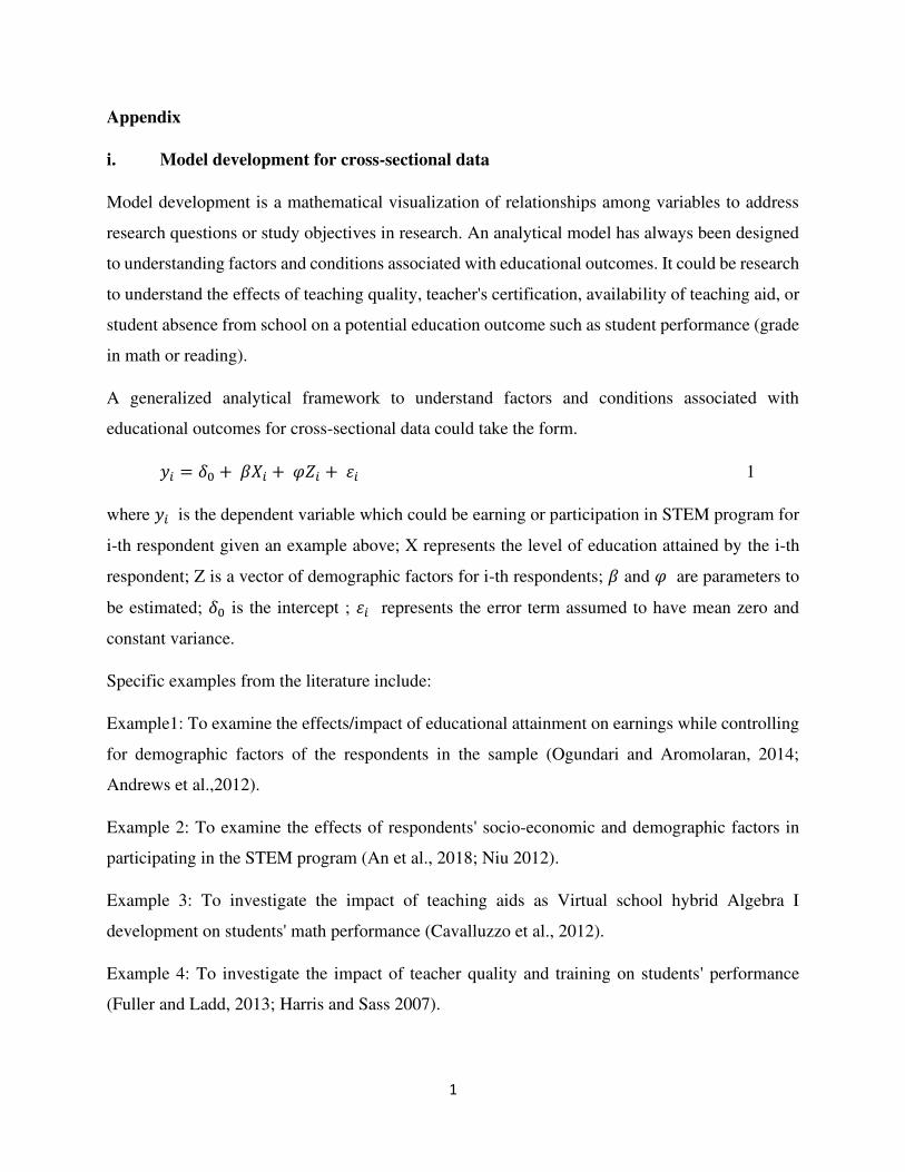
1

Appendix

i. Model development for cross-sectional data

Model development is a mathematical visualization of relationships among variables to address

research questions or study objectives in research. An analytical model has always been designed

to understanding factors and conditions associated with educational outcomes. It could be research

to understand the effects of teaching quality, teacher's certification, availability of teaching aid, or

student absence from school on a potential education outcome such as student performance (grade

in math or reading).

A generalized analytical framework to understand factors and conditions associated with

educational outcomes for cross-sectional data could take the form. 𝑦𝑖 = 𝛿0 + 𝛽𝑋𝑖 + 𝜑𝑍𝑖 + 𝜀𝑖 1

where 𝑦𝑖 is the dependent variable which could be earning or participation in STEM program for

i-th respondent given an example above; X represents the level of education attained by the i-th

respondent; Z is a vector of demographic factors for i-th respondents; 𝛽 and 𝜑 are parameters to

be estimated; 𝛿0 is the intercept ; 𝜀𝑖 represents the error term assumed to have mean zero and

constant variance.

Specific examples from the literature include:

Example1: To examine the effects/impact of educational attainment on earnings while controlling

for demographic factors of the respondents in the sample (Ogundari and Aromolaran, 2014;

Andrews et al.,2012).

Example 2: To examine the effects of respondents' socio-economic and demographic factors in

participating in the STEM program (An et al., 2018; Niu 2012).

Example 3: To investigate the impact of teaching aids as Virtual school hybrid Algebra I

development on students' math performance (Cavalluzzo et al., 2012).

Example 4: To investigate the impact of teacher quality and training on students' performance

(Fuller and Ladd, 2013; Harris and Sass 2007).

2

ii. Analytical model development for Panel data

The availability of a longitudinal survey that extends beyond one period or extends back to 2 to

more years provides an opportunity to examine the trends in the potential outcomes of interest. In

this case, there is a need to remodify the above model specification to consider the data's time

dimension, as shown below. 𝑦𝑖𝑡 = 𝛽𝑋𝑖𝑡 + 𝜑𝑍𝑖 + 𝛿𝑖 + 𝜀𝑖𝑡 2

where 𝑦𝑖𝑡 is the dependent variable for i-th respondent in the t period, which could be students test

scores ( See Fuller and Ladd, 2013); Xit represent time-varying explanatory variables which could

be an indicator of teacher quality and Zi is a vector of time-invariant control variables such gender,

ethnicity, individual, country, regional or specific fixed effect, etc. for i-th respondents; 𝛽 and 𝜑

are parameters to be estimated; 𝛿𝑖 is the unobserved heterogeneity; 𝜀𝑖𝑡 represents the idiosyncratic

error term.

iii. Analytical model development for estimating causal Inference

The evaluation of the impact of programs such as pre-school, remedial education, or early learning

programs, among others, on cognitive outcomes (e.g., reading scores, math scores) is important to

guide policymakers on whether these programs worth investment or assessing the effectiveness of

these programs. A typical model specification to evaluate the impact of programs on potential

outcomes of interest as often used in agriculture, health, education, transportation, etc., can be

specified. 𝑦𝑖 = 𝛿0 + 𝛽𝑇 + 𝜑𝑍𝑖 + 𝜀𝑖 3

where 𝑦𝑖 represents potential outcome ( e.g., test score) for i-th respondent; T is the indicator

representing assignment into treatment for the i-th respondent1; Z is a vector of socio-demographic

factors for i-th respondents; 𝛽 and 𝜑 are parameters to be estimated, where 𝛽 represents estimated

impact of interest ; 𝛿0 is the intercept ; 𝜀𝑖 represents the error term assumed to have mean zero

and constant variance.

1 It is important to note that, in the evaluation literature, “treatment” conventionally refers to the individuals who participate in the program.

3

While equation 3 is referred to as an outcome equation, the selection equation similar to the first

stage equation described in Heckman (1979) or first hurdle described in Cragg (1971) can be

defined below 𝑇𝑖 = Ω0 + 𝜎𝑍 + 𝜋𝑋𝑖 + 𝜐 4

where 𝑇𝑖 and 𝑍 are as defined earlier; X is additional variables that could be a valid instrument to

identify the process. 𝜎, Ω0, and 𝜋 are parameters to be estimated. 𝜐 is the error term assumed to

have mean zero and constant variance.

With the availability of panel data, equation 3 can be re-specified to reflect this as follows 𝑦𝑖𝑡 = 𝜑0 + 𝜂𝑇 + 𝜏𝑍𝑖𝑡 + 𝜁𝑖𝑡 , t=1, 2,……Time 5

where 𝑦, T, and Z are as defined earlier; 𝜑, 𝜂, 𝑎𝑛𝑑 𝜏 are parameters to be estimated ; 𝜁𝑖𝑡

are random disturbances.

The difference in difference (DiD) specification in Equation 5 can be defined as 𝑦𝑖𝑡 = 0 + 𝜗𝑇𝑖𝑚𝑒 + 𝜋𝑇 + 𝜏(𝑇𝑖𝑚𝑒 ∗ 𝑇) + 𝜏𝑍𝑖𝑡 + Ω𝑖𝑡 , t=1, 2,……Time 6

where 𝑦, T, and Z are as defined earlier; 𝜏 is the coefficient of DiD estimator; Ω𝑖𝑡 are the random

disturbances.

iv. Endogeneity problem in education production function: The role of instrumental

variable estimator

There are five commonly encountered situations where the regression model's endogeneity

problem exists. This includes simultaneous causality, omitted variable, errors in variables, sample

selection, and functional form misspecification. The existence of endogeneity problems in

regression biased the policy results, so education researchers must consider this in their research.2

A typical example of this is estimating the effect of attendance on student performance, or the

impact of education attained on earnings, or the impact of programs such as early learning

education on student performance. The problem here is that attendance, education achieved, or

2 There is a test often perform to test whether a regressor is actually endogenous and is called Durbin-Wu Hausman

test. There are some regressors that are obviously predetermine from economic theory that are endogenous. Example

of this is education in this example. Education or regressors generally can be tested using this Durbin-Wu Hausman

test.

4

participation in early learning education is not exogenous (or is endogenous), which violates the

classical assumption of linear regression that an explanatory variable should be exogenous. In

practice, what this means is that attendance, education attained, or participation in early learning

education should not be correlating with the error terms. The existence of the endogeneity problem

asymptotically biases the results.

The endogeneity problem is widespread in education research, and researchers have not been pay

attention to this. Equation 3, with treatment assignment T- representing early learning participation

or STEM program participation, is a typical example of an endogeneity problem due to selection

bias. The specification below is the impact of education achieved by year of schooling on earnings

while controlling for respondents' characteristics. 𝐸𝑎𝑟𝑛𝑖𝑛𝑔𝑠𝑖 = 0 + 𝜗𝐸𝑑𝑢𝑐𝑎𝑡𝑖𝑜𝑛𝑌𝑒𝑎𝑟 + 𝜏𝑍𝑖 + Ω𝑖 7

where Earnings is the wage rate per hour; EducationYear is the year of schooling attained; Z is

respondents' characteristics such as age, gender, ethnicity, etc. 𝜗, , and 𝜏 are parameters to be

estimated; Ω𝑖𝑡 is a random disturbance. The parameter of interest here is 𝜗, which captures returns

to education.

The problem here is that year of education is endogenous because education attained depends on

so many factors such as ability, parent education, school quality, etc., which are omitted in equation

7, perhaps due to lack of data. Therefore, the estimation of equation 7 without controlling for this

problem bias the estimated return to education 𝜗 for policy.

There are various approaches to mitigate the endogeneity problem in IV regression, including two-

stage least square (2SLS), 2 stage GMM, and Limited information maximum likelihood (LIML)

estimators. While 2SLS and 2 step GMM are very popular among researchers, the computational

difficulty of LIML makes limits its usage. Unlike 2SLS, 2 stage GMM is robust to

heteroskedasticity. In the absence of heteroskedasticity, 2SLS is consistent as 2 stage GMM>

Other methods include control function or, in some cases, the Heckman selection model depending

on the data generating process. We discussed Heckman's selection bias in detail in the main text.

Our focus here is to describe the specification of 2SLS for IV regression.

The solution to the endogeneity of education year in equation 7 above is to find an instrument (m)

that is correlated with earnings but not correlated with the error term (i.e., Cov (earnings, m)≠0 &

5

Cov(m, Ω𝑖)=0).3 The IV regression uses the instrument to estimate first stage regression where

endogenous regressor (e.g., EducationYear) is expressed as a function of the instrument (e.g., m)

and other explanatory variables (e.g., Z), as shown below. 𝐸𝑑𝑢𝑐𝑎𝑡𝑖𝑜𝑛𝑌𝑒𝑎𝑟 = 𝜐0 + 𝜎𝑚 + 𝛼𝑍𝑖 + 𝛷𝑖 8

After that, the predicted value from the first stage (equation 8) denoted by 𝐸𝑑𝑢𝑐𝑎𝑡𝑖𝑜𝑛𝑌𝑒𝑎𝑟

replaces the original variable in equation 7 as specified below 𝐸𝑎𝑟𝑛𝑖𝑛𝑔𝑠𝑖 = 𝜚0 + 𝜁 𝐸𝑑𝑢𝑐𝑎𝑡𝑖𝑜𝑛𝑌𝑒𝑎𝑟 + 𝜍𝑍𝑖 + 𝜖𝑖 9

Equation 9 is called a reduced equation. Unlike 𝜗 in equation 7, the estimated return to education 𝜁 in equation 9 is unbiased and reliable for policy inferences since the instrument (m) introduces

an element of randomness into the assignment, which approximates the effect of an experiment

(Vandenberghe and Robin, 2004). This explained why the IV estimator is also a popular causal

inference method for mitigating selection bias problems in data. We discuss this in detail in the

main text. Besides, the linear IV estimators described above, it is important to note that it can be

extended to a binary response-dependent variable such as IV probit for binary variable or IV Tobit

for censored dependent variable.

As noted by Woodridege (2002), the problem here is finding the instrument (m) that is uncorrelated

with the error term of the original equation (i.e., Cov(m, Ω𝑖)=0) and at the same time correlated

with the endogenous variable (i.e., Cov(m, Education Year)≠0). Thus, it is vital to check the

validity of the instrument (m), also called the relevance test, and a test of overidentification using

the Sargan test. The instrument's relevance is based on the estimated F statistics from the first stage

(equation 8). As a rule of thumb, a critical F-statistic of 10 and above shows that the instrument is

sufficiently strong (Wooldrideg 2002). With the instruments' k-number, the Sargan test is essential

to assess whether the instruments are over-identified or just identified. A detailed discussion of

this method is available in Angrist and Pischke (2008).

Vandenberghe and Robin (2004) evaluate the effectiveness of private education Vs. Public

education on student performance across countries, where the authors used a dummy, equals 1 if

a pupil attends a school located in a big city and 0 otherwise. Gottfried (2010) evaluates the effect

3 The illustration here is similar to the one describes in the footnote 3.

6

of attendance on student achievement. The author used the distance in exact miles a student lives

from school as an instrument to control for the endogeneity of attendance in the study. Card (1999)

employed IV regression to estimate the effect of education on earnings. The author used a dummy,

equals one if born in the university's neighborhood, and 0 otherwise as an instrument for years of

schooling in the study.