Embed Size (px)
Citation preview
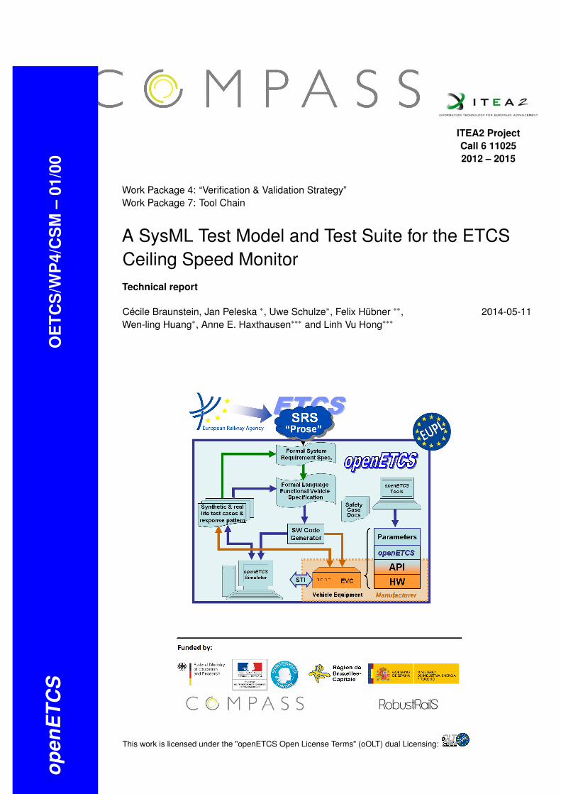
open
ETC
SO
ETC
S/W
P4/
CS
M–
01/0
0
ITEA2 ProjectCall 6 110252012 – 2015
Work Package 4: “Verification & Validation Strategy”Work Package 7: Tool Chain
A SysML Test Model and Test Suite for the ETCSCeiling Speed MonitorTechnical report
Cécile Braunstein, Jan Peleska ∗, Uwe Schulze∗, Felix Hübner ∗∗,Wen-ling Huang∗, Anne E. Haxthausen∗∗∗ and Linh Vu Hong∗∗∗
2014-05-11
This work is licensed under the "openETCS Open License Terms" (oOLT) dual Licensing:

This page is intentionally left blank
OETCS/WP4/CSM – 01/00 1
Work Package 4: “Verification & Validation Strategy”Work Package 7: Tool Chain
OETCS/WP4/CSM – 01/002014-05-11
A SysML Test Model and Test Suite for the ETCSCeiling Speed MonitorTechnical report
Cécile Braunstein, Jan Peleska ∗, Uwe Schulze∗ and Felix Hübner ∗∗
University Bremen
Wen-ling Huang∗
University of Hamburg and University of Bremen, Germany
Anne E. Haxthausen∗∗∗ and Linh Vu Hong∗∗∗
DTU Computer Technical University of Denmark
- ∗ The authors’ research is funded by the EU FP7 COMPASS project under grant agreement no.287829.- ∗∗ The author’s research is funded by Siemens in the context of the SyDE Graduate School on System Design- ∗∗∗ The authors’ research is funded by the RobustRailS project funded by the Danish Council for StrategicResearch.
Technical Report
Prepared for openETCS@ITEA2 Project
This work is licensed under the "openETCS Open License Terms" (oOLT).

OETCS/WP4/CSM – 01/00 2
Abstract: This technical report contributes to the openETCS project, work packages WP4 –Verification & Validation Strategy, and WP7 – Tool Chain.
In this technical report, a detailed model description of a train control system application isgiven – this has been elaborated in the context of work package WP4 of the openETCS project.The application consists of the ceiling speed monitoring (CSM) function for the EuropeanVital Computer, which is the main onboard controller for trains conforming to the EuropeanTrain Control System specification. The model is provided in SysML, and it is equipped witha formal semantics that is consistent with the (semi formal) SysML standard published bythe Object Management Group (OMG). The model and its description are publicly availableon http://www.mbt-benchmarks.de, a website dedicated to the publication of models that areof interest for the model-based testing (MBT) community, and may serve as benchmarks forcomparing MBT tool capabilities. The model described here is of particular interest for analysingthe capabilities of equivalence class testing strategies. The CSM application inputs velocity valuesfrom a domain which could not be completely enumerated for test purposes with reasonableeffort.
We describe a novel method for equivalence class testing that – despite the conceptually infinitecardinality of the input domains – is capable to produce finite test suites that are exhaustive undercertain hypotheses about the internal structure of the system under test. In the context of workpackage WP7, this strategy has been implemented in the RT-Tester test automation tool whichhas been made available for the openETCS project as part of WP7.
Keywords Model-based testing, Equivalence class partition testing, UML/SysML, EuropeanTrain Control System ETCS, Ceiling Speed Monitoring
Disclaimer: This work is licensed under the "openETCS Open License Terms" (oOLT) dual Licensing: European Union PublicLicence (EUPL v.1.1+) AND Creative Commons Attribution-ShareAlike 3.0 – (cc by-sa 3.0)
THE WORK IS PROVIDED UNDER openETCS OPEN LICENSE TERMS (oOLT) WHICH IS A DUAL LICENSE AGREEMENT IN-CLUDING THE TERMS OF THE EUROPEAN UNION PUBLIC LICENSE (VERSION 1.1 OR ANY LATER VERSION) AND THETERMS OF THE CREATIVE COMMONS PUBLIC LICENSE ("CCPL"). THE WORK IS PROTECTED BY COPYRIGHT AND/OROTHER APPLICABLE LAW. ANY USE OF THE WORK OTHER THAN AS AUTHORIZED UNDER THIS OLT LICENSE OR COPY-RIGHT LAW IS PROHIBITED.
BY EXERCISING ANY RIGHTS TO THE WORK PROVIDED HERE, YOU ACCEPT AND AGREE TO BE BOUND BY THE TERMSOF THIS LICENSE. TO THE EXTENT THIS LICENSE MAY BE CONSIDERED TO BE A CONTRACT, THE LICENSOR GRANTSYOU THE RIGHTS CONTAINED HERE IN CONSIDERATION OF YOUR ACCEPTANCE OF SUCH TERMS AND CONDITIONS.
http://creativecommons.org/licenses/by-sa/3.0/http://joinup.ec.europa.eu/software/page/eupl/licence-eupl
This work is licensed under the "openETCS Open License Terms" (oOLT).

OETCS/WP4/CSM – 01/00 3
Table of Contents1 Introduction................................................................................................................. 1
1.1 A Test Model for the ETCS Ceiling Speed Monitor ..................................................... 1
1.2 Equivalence Class Partition Testing for the CSM........................................................ 1
1.3 Fault Models and Completeness Results ................................................................. 2
2 The Ceiling Speed Monitoring Function – Functional Objectives ............................................. 2
3 Model Description ........................................................................................................ 2
3.1 Model Availability ................................................................................................ 2
3.2 Model Components ............................................................................................. 3
3.3 Model Semantics – Overview ................................................................................ 3
3.4 Interfaces.......................................................................................................... 4
3.5 SUT Attributes and Operations .............................................................................. 5
3.6 Requirements .................................................................................................... 8
3.7 Behavioural Specification ..................................................................................... 8
3.8 Requirements Tracing ......................................................................................... 14
4 Formal Semantics – the Transition Relation....................................................................... 18
4.1 Semantic Definition Scope................................................................................... 18
4.2 State Transition System Semantics ........................................................................ 18
4.3 State Space ..................................................................................................... 18
4.4 Quiescent and Transient States ............................................................................ 19
4.5 Initial State ....................................................................................................... 19
4.6 Transition Relation – General Construction Rules ..................................................... 20
4.7 Transition Relation for the CSM............................................................................. 23
4.7.1 Propositions Specifying Internal State and Outputs – ξi. ............................................... 23
4.7.2 Propositions Specifying Input Conditions for Quiescent Classes – ϕIi . .............................. 23
4.7.3 Quiescent Post-State Condition – qpsc. .................................................................... 24
4.7.4 Transient Post-State Condition – tpsc. ...................................................................... 24
4.7.5 Transient State Input Conditions – ϕIq,i. ..................................................................... 24
5 Input Equivalence Class Partitionings .............................................................................. 27
5.1 Strategy Overview ............................................................................................. 27
5.1.1 I/O-Equivalence................................................................................................... 27
5.1.2 Input Equivalence Class Partitions........................................................................... 27
5.1.3 Fault Model ........................................................................................................ 28
5.1.4 Complete Test Strategy ......................................................................................... 29
5.2 Practical Construction of Input Equivalence Classes and Associated Partitionings ........... 29
5.2.1 CSM I/O-Equivalence Classes ................................................................................ 29
5.2.2 CSM Input Equivalence Class Partitions ................................................................... 30
5.3 Inter-Class Transitions ........................................................................................ 31
6 CSM Fault Model ........................................................................................................ 31
7 Complete Test Suites for the CSM .................................................................................. 33
7.1 Test Suite Construction – Overview ....................................................................... 33
7.2 Application of the W-Method ................................................................................ 33
8 Test Strength.............................................................................................................. 35
8.1 Test Strength Assessment ................................................................................... 35
8.2 Example 1........................................................................................................ 36
8.3 Example 2........................................................................................................ 36
8.4 Example 3........................................................................................................ 38
9 Heuristics for Constructing IECP Refinements ................................................................... 40
This work is licensed under the "openETCS Open License Terms" (oOLT).
OETCS/WP4/CSM – 01/00 4
9.1 IECP Refinements for the CSM............................................................................. 40
9.2 Overview of the Refinement Concept ..................................................................... 41
9.3 Requirements-based IECP Refinement .................................................................. 41
9.3.1 Requirements-related Case Distinctions ................................................................... 41
9.3.2 Construction of the Requirements-based IECP Refinement........................................... 42
9.3.3 Discussion ......................................................................................................... 47
9.4 Boundary Value IECP Refinement ......................................................................... 47
9.5 IECP Refinement by Sub-paving ........................................................................... 49
9.6 Effects of IECP Refinements on W-Method Application .............................................. 49
10 Test Procedures.......................................................................................................... 52
10.1 Test Automation Tool .......................................................................................... 52
10.2 Test Categories ................................................................................................. 52
10.3 Tests of Categories 1 — 4 ................................................................................... 52
10.4 Tests of Category 5 – IECP Tests .......................................................................... 54
11 Related Work ............................................................................................................. 56
12 Conclusion ................................................................................................................ 57
13 Ongoing and Future Work ............................................................................................. 57
References ....................................................................................................................... 58
This work is licensed under the "openETCS Open License Terms" (oOLT).

OETCS/WP4/CSM – 01/00 5
Figures and Tables
Figures
Figure 1. System interface of the ceiling speed monitor. ..................................................................... 4
Figure 2. Block diagram with CSM (sequential behaviour)................................................................... 6
Figure 3. System requirements diagram. ........................................................................................ 9
Figure 4. Ceiling speed monitoring – top-level state machine.............................................................. 11
Figure 5. Ceiling speed monitoring state machine. ........................................................................... 12
Figure 6. Graphical representation of the «satisfy» relation in a state machine diagram............................ 16
Figure 7. DFSM abstractions of the CSM, with configuration cases sb0 ∈ {0, 1}....................................... 34
Figure 8. Faulty SUT – Example 1. ............................................................................................... 37
Figure 9. Faulty SUT – Example 2. ............................................................................................... 39
Figure 10. Faulty SUT – Example 3. ............................................................................................. 40
Tables
Table 1. Requirements for the ceiling speed monitoring function.......................................................... 10
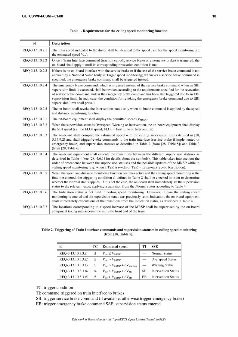
Table 2. Triggering of Train Interface commands and supervision statuses in ceiling speed monitoring(from [28, Table 5]). ................................................................................................................... 10
Table 3. Revocation of Train Interface commands and supervision statuses in ceiling speed monitoring(from [28, Table 6]). ................................................................................................................... 11
Table 4. Transitions between supervision statuses in ceiling speed monitoring (from [28, Table 7]).............. 11
Table 5. Requirements links to the SysML Elements......................................................................... 15
Table 6. Constraints related to complex requirements listed in Table 5. ................................................. 17
Table 7. Identification of basic states in machine CSM_ON ................................................................ 19
Table 8. DFSM Transition Table.................................................................................................... 32
Table 9. Input Alphabet AI .......................................................................................................... 32
Table 10. DFSM states and associated I/O-equivalence classes. ........................................................ 33
Table 11. Extended input alphabet A′I satisfying AI ⊆ A′I . ................................................................. 46
Table 12. Extended input alphabet AI containing boundary values. ..................................................... 50
Table 13. Test procedures .......................................................................................................... 53
Table 14. Requirement-based Test procedures ............................................................................... 54
Table 15. TP-002-OnlyCSM_ON Test suite..................................................................................... 54
Table 16. TP-002-OnlyCSM_ON-NOSB Test suite ........................................................................... 54
Table 17. Mutants experiments results .......................................................................................... 55
Table 18. Test sequences that kills the mutant ................................................................................ 55
This work is licensed under the "openETCS Open License Terms" (oOLT).

OETCS/WP4/CSM – 01/00 6
This work is licensed under the "openETCS Open License Terms" (oOLT).
OETCS/WP4/CSM – 01/00 1
1 Introduction
1.1 A Test Model for the ETCS Ceiling Speed Monitor
In 2011 the model-based testing benchmarks website www.mbt-benchmarks.org has been createdwith the objective to publish test models that may serve as challenges or benchmarks for validatingtesting theories and for comparing the capabilities of model-based testing (MBT) tools [24]. Inthis technical report a novel contribution to this website is presented, a SysML model of theCeiling Speed Monitor (CSM) which is part of the European Vital Computer (EVC), the onboardcontroller of trains conforming to the European Train Control System (ETCS) standard [6]. InSection 2 the functional objectives for the CSM are described, and in Section 3 the detailedmodel description is provided.
The static and behavioural semantics of SysML models have been defined in [21, 22] in asemi-formal way, leaving certain “semantic variation points” open, so that they can be adjustedaccording to project-specific requirements. For automated model-based testing, however, astrictly formal semantics is required, so that concrete test data can be calculated from the model’stransition relation using constraint solving techniques [12]. We therefore describe in Section 4how a formal behavioural semantics is derived for the CSM model and present the associatedtransition relation in propositional form.
We use state transition systems (STS) for encoding the operational semantics of concrete mod-elling formalisms like SysML. STS are widely known from the field of model checking [5],because their extension into Kripke Structures allows for effective data abstraction techniques.The latter are also applied for equivalence class testing. Since state transition systems are a meansfor semantic representation, testing theories elaborated for STS are applicable for all concreteformalisms whose behavioural semantics can be expressed by STS. In [13] it is shown how thesemantics of general SysML models and models of a process algebra are encoded as STS. Inthis technical report we illustrate how this is achieved for the concrete case of the CSM SysMLmodel.
1.2 Equivalence Class Partition Testing for the CSM
The CSM represents a specific test-related challenge: its behaviour depends on actual and allowedspeed, and these have conceptually real-valued data domains, so that – even when discretisingthe input space – it would be infeasible to exercise all possible combinations of inputs on thesystem under test (SUT). Therefore equivalence class partition (ECP) testing strategies have tobe applied for testing the CSM. While these strategies are well-adopted in a heuristic mannerin today’s industrial test campaigns, practical application of equivalence class testing still lacksformal justification of the equivalence classes selected and the sequences of class representativesselected as test cases: standard text books used in industry, for example [27], only explain thegeneration of input equivalence class tests for systems, where the SUT reaction to an inputclass representative is independent on the internal state. Moreover, the systematic calculationof classes from models, as well as their formal justification with respect to test strength andcoverage achieved, is not yet part of today’s best practices in industry.
In contrast to this, formal approaches to equivalence class testing have been studied in the formalmethods communities; references to these results are given in Section 11. In the second mainpart of this report (Section 5) we therefore describe a recent formal technique for equivalenceclass testing and its application to testing the CSM. The theoretical foundations of this strategyhave been published by two of the authors in [12]. This technical report illustrates its practical
This work is licensed under the "openETCS Open License Terms" (oOLT).

OETCS/WP4/CSM – 01/00 2
application and presents first evaluation details using a prototype implementation in an existingMBT tool; the ECP tests are compared to test results obtained when applying other MBT coveragestrategies, such as transition cover or MC/DC coverage (Section 10).
1.3 Fault Models and Completeness Results
Our ECP strategy introduces test suites depending on fault models. This well adopted notion hasfirst been introduced in the field of finite state machine (FSM) testing [25], but is also applicableto other formal modelling techniques. A fault model consists of a reference model, a conformancerelation and a fault domain. The latter is a collection of models whose behaviour may or maynot be consistent to the reference model in the sense of the conformance relation. The test suitesgenerated by the ECP strategy described here are complete with respect to the given fault model:each system of the fault domain which conforms to the reference model will pass all the generatedtests (this means that the test suite is sound), and each system in the fault domain that violatesthe conformity to the reference model will fail at least once when tested according to the testsuite (the test suite is exhaustive).
2 The Ceiling Speed Monitoring Function – Functional Objectives
The European Train Control System ETCS relies on the existence of an onboard controller intrain engines, the European Vital Computer EVC. Its functionality and basic architectural featuresare described in the public ETCS system specification [6]. One functional category of the EVCcovers aspects of speed and distance monitoring, to accomplish the “. . . supervision of the speedof the train versus its position, in order to assure that the train remains within the given speedand distance limits.” [28, 3.13.1.1]. Speed and distance monitoring is decomposed into threesub-functions [28, 3.13.10.1.2], where only one out of these three is active at a point in time:
1. Ceiling speed monitoring (CSM) supervises the observance of the maximal speed allowedaccording to the current most restrictive speed profile (MRSP). CSM is active while thetrain does not approach a target (train station, level crossing, or any other point that must bereached with predefined speed).
2. Target speed monitoring (TSM) supervises the observance of the maximal distance-dependingspeed, while the train brakes to a target, that is, a location where a given predefined speed(zero or greater zero) must be met.
3. Release speed monitoring (RSM) applies when the special target “end of movement authority(EOA)” is approached, where the train must come to a stop. RSM supervises the observanceof the distance-depending so-called release speed, when the train approaches the EOA.
In this technical report we present a complete formal model of the CSM function, with theobjective to derive a complete test suite from this model (Section 5).
3 Model Description
3.1 Model Availability
The ceiling speed monitor has been modelled using the OMG Systems Modeling Language (OMGSysMLT M) [21]. The complete model is available for download under http://www.mbt-benchmarks.org.This is a website dedicated to the publication of test models possessing features that are of generalinterest for researchers and practitioners in the field of model-based testing (MBT). Moreover,
This work is licensed under the "openETCS Open License Terms" (oOLT).

OETCS/WP4/CSM – 01/00 3
the models may serve as benchmarks for comparing test automation tools with respect to teststrength and tool performance. This has been further motivated in [24], where also suggestionsfor MBT benchmarks are given. In this section, we give a comprehensive introduction into theformal model.
3.2 Model Components
According to the model-based testing approach applied in this report, UML/SysML test modelsare structured into the following basic components.
1. A package containing the system requirements (Fig. 3),
2. A block diagram (Fig. 1) identifying
• the system under test (SUT),
• its interface to the operational environment, and
• the test environment (TE) simulating the “real” operational environment during testexecution,
3. Subordinate block diagrams refining the internal structure of the SUT (Fig. 2) and the TE,respectively,
4. State machines associated with the leaf blocks of the structural decompositions of SUT(Fig. 4) and TE, and
5. Operations associated with blocks. These are referenced by state machines, when evaluatingguard conditions or performing actions.
3.3 Model Semantics – Overview
The detailed formal behavioural semantics of SysML test models has been described in [13,pp. 88]. This semantics is consistent with the standards [22, 21], but fixes certain semanticvariation points in ways that are admissible according to the standards. In this technical report,however, the semantic details will be explained as far as they are relevant for understanding themodel presented here: in the present section, the behavioural semantics of the CSM model isinformally explained, and in Section 4, the formal model semantics is specified by presenting itstransition relation.
The leaf components of the structural model decomposition execute concurrently. For themodel under consideration the SUT operates in a sequential manner, but concurrently with itsenvironment. In this test model, the behaviour of the TE is undetermined; this is interpretedin the way that every possible sequence of input vectors to the SUT would be allowed. Thisassumption is reasonable for the example considered here: due to robustness requirements, theceiling speed monitor must be able to cope with input sequences that may be unreasonable froma physical point of view. TE components are introduced in situations where only certain types ofinteractions between operational environment and SUT are possible.
The model executes according to the run-to-completion semantics defined for state machinesin [22]. The model is in a quiescent (or stable) state, if no transition can be executed withoutan input change. In a quiescent model state, inputs may be changed. If these changes enablea transition, the latter is executed. Since our SUT model is deterministic – this is typical for
This work is licensed under the "openETCS Open License Terms" (oOLT).
OETCS/WP4/CSM – 01/00 4
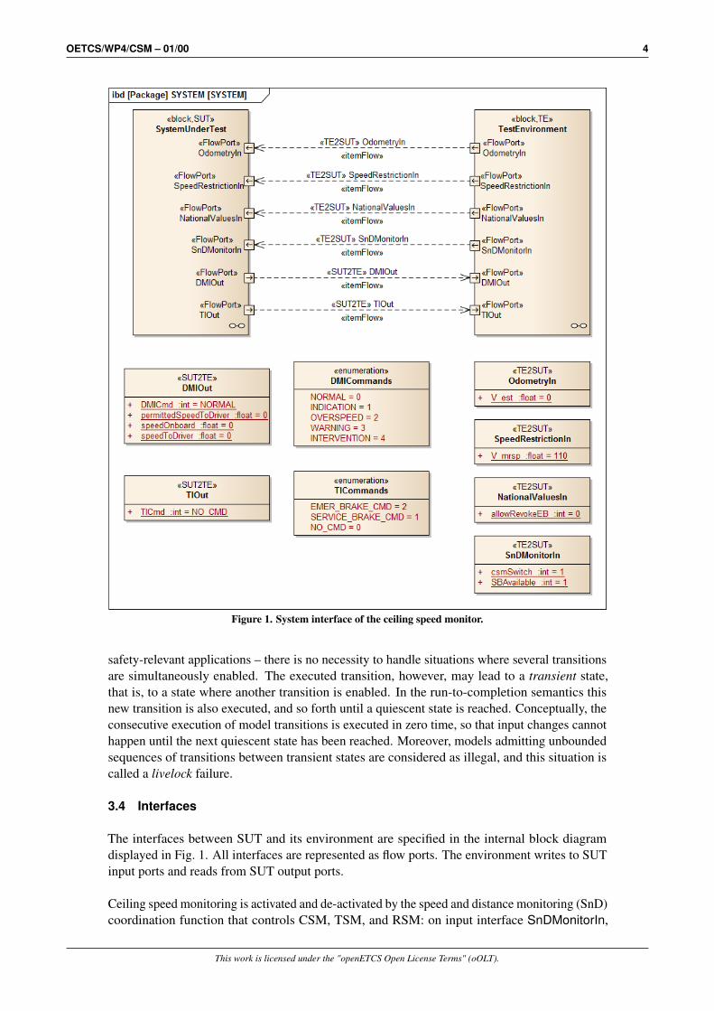
Figure 1. System interface of the ceiling speed monitor.
safety-relevant applications – there is no necessity to handle situations where several transitionsare simultaneously enabled. The executed transition, however, may lead to a transient state,that is, to a state where another transition is enabled. In the run-to-completion semantics thisnew transition is also executed, and so forth until a quiescent state is reached. Conceptually, theconsecutive execution of model transitions is executed in zero time, so that input changes cannothappen until the next quiescent state has been reached. Moreover, models admitting unboundedsequences of transitions between transient states are considered as illegal, and this situation iscalled a livelock failure.
3.4 Interfaces
The interfaces between SUT and its environment are specified in the internal block diagramdisplayed in Fig. 1. All interfaces are represented as flow ports. The environment writes to SUTinput ports and reads from SUT output ports.
Ceiling speed monitoring is activated and de-activated by the speed and distance monitoring (SnD)coordination function that controls CSM, TSM, and RSM: on input interface SnDMonitorIn,
This work is licensed under the "openETCS Open License Terms" (oOLT).
OETCS/WP4/CSM – 01/00 5
variable csmSwitch specifies whether ceiling speed monitoring should be active (csmSwitch =
1) or passive, since target or release speed monitoring is being performed (csmSwitch = 0).Furthermore, this interface carries variable SBAvailable which has value 1, if the train is equippedwith a service brake. This brake is then used for slowing down the train if it has exceeded themaximal speed allowed, but not yet reached the threshold for an emergency brake intervention. IfSBAvailable = 0, the emergency brake shall be used for slowing down the train in this situation.Input SBAvailable is to be considered as a configuration parameter of the train, since it dependson the availability of the service brake hardware. Therefore this value can be freely selected atstart-of-test, but must remain constant during test execution.
Input interface OdometryIn provides the current speed value estimated by the odometer equip-ment in variable Vest. Input interface SpeedRestrictionIn provides the current maximal velocitydefined by the most restrictive speed profile in variable VMRSP. Input interface NationalVal-uesIn provides a control flag for the ceiling speed monitor: variable allowRevokeEB is 1, ifafter an emergency brake intervention the brake may be automatically released as soon as theestimated velocity of the train is again less or equal to the maximal speed allowed. Otherwise(allowRevokeEB = 0) the emergency brakes must only be released after the train has come to astandstill (Vest = 0). This input parameter is called a “national value”, because it may changewhen a train crosses the boundaries between European countries, due to their local regulations.
Output interface DMIOut sends data from the SUT to the driver machine interface (DMI). Itcarries five variables. DMICmd is used to display the supervision status to the train engine driver:Value INDICATION may be initially present when CSM is activated, but will be immediatelyoverridden by one of the values NORMAL, OVERSPEED, WARNING, or INTERVENTION,as soon as ceiling speed monitoring becomes active. Value NORMAL is written by the SUT tothis variable as long as the ceiling speed is not violated by the current estimated speed. ValueOVERSPEED has to be set by the CSM as soon as condition VMRSP < Vest becomes true. If thespeed increases further (the detailed conditions are described below), the indication changes fromOVERSPEED to WARNING, and from there to INTERVENTION. The latter value indicatesthat either the train is slowed down until it is back in the normal speed range, or the emergencybrake has been triggered to stop the train. Furthermore, interface DMIOut contains the followingspeed-related variables that are displayed as y/t-diagrams on the DMI.
• speedToDriver: the current estimated speed as given by variable Vest.
• permittedSpeedToDriver: the permitted maximal speed as given by the most restrictive speedprofile VMRSP.
• speedOnBoard: maximal speed allowed (VMRSP) as long as the train does not overspeed.Otherwise it carries values VMRSP +δ, where δ > 0 specifies the margin from VMRSP to servicebrake intervention and is calculated as described below.
Output interface TIout specifies the train interface from the CSM to the brakes, using variableTICmd. If TICmd = NO_CMD, both service brakes (if existent) and emergency brakes arereleased. If TICmd = SERVICE_BRAKE_CMD, the service brake is activated. If TICmd =
EMER_BRAKE_CMD, the emergency brake is triggered.
3.5 SUT Attributes and Operations
The CSM is modelled as an application with sequential behaviour. Therefore the SUT block onthe top-level interface diagram (Fig. 1) is refined into another block diagram that just carries theSUT, as shown in Fig. 2.
This work is licensed under the "openETCS Open License Terms" (oOLT).

OETCS/WP4/CSM – 01/00 6
Figure 2. Block diagram with CSM (sequential behaviour).
This work is licensed under the "openETCS Open License Terms" (oOLT).
OETCS/WP4/CSM – 01/00 7
As shown there, the SUT uses a local attribute sbiCmd which carries value SERVICE_BRAKE_CMD,if the service brake should be used for slowing down the train to the admissible speed. If thevalue EMER_BRAKE_CMD is assigned to sbiCmd, the emergency brake will be triggered inthis situation.
Operations dV_warning(float), dV_sbi(float), dV_ebi(float) return values that are used to de-termine whether a warning should be indicated to the train engine driver (Vest > VMRSP +
dVwarning(VMRSP)), a service brake intervention should be triggered (Vest > VMRSP+dVsbi(VMRSP)),or the emergency brake should be activated (Vest > VMRSP + dVebi(VMRSP)). In each case, thecalculation is performed according to the pattern
dVx(VMRSP) =
min{dVxmin + Cx · (VMRSP − Vxmin), dVxmax}
if VMRSP > Vxmin
dVxmin
if VMRSP ≤ Vxmin
(1)
which has been defined in [28, 3.13.9.2.3]. Here x can be replaced by warning, sbi (SBI = servicebrake intervention), and ebi (EBI = Emergency Brake Intervention), and Cx is defined by
Cx =dVxmax − dVxmin
Vxmax − Vxmin
The following minimal and maximal values apply [28, A.3.1]:
dVwarningmin = 4 dVsbimin = 5.5 dVebimin = 7.5
dVwarningmax = 5 dVsbimax = 10 dVebimax = 15
Vwarningmin = 110 Vsbimin = 110 Vebimin = 110
Vwarningmax = 140 Vsbimax = 210 Vebimax = 210
Inserting these values into Equation (1) results in
dVwarning(VMRSP) =
min{ 13 + 130 · VMRSP, 5} if VMRSP > 110
4 if VMRSP ≤ 110(2)
dVsbi(VMRSP) =
min{0.55 + 0.045 · VMRSP, 10} if VMRSP > 110
5.5 if VMRSP ≤ 110(3)
dVebi(VMRSP) =
min{−0.75 + 0.075 · VMRSP, 15} if VMRSP > 110
7.5 if VMRSP ≤ 110(4)
Operations calc_speed_to_driver() and calc_permitted_speed_to_driver() support the display ofthe current estimated speed and the maximum speed, respectively, at the driver machine interfaceby performing assignments to output variables:
speedToDriver = Vest
permittedSpeedToDriver = VMRSP
This work is licensed under the "openETCS Open License Terms" (oOLT).

OETCS/WP4/CSM – 01/00 8
Operation calc_speed_onboard() displays the maximal speed VMRSP specified by the most re-strictive speed profile in DMI interface variable speedOnBoard, as long as the train is notoverspeeding. As soon as Vest > VMRSP, this function calculates the service brake interventionspeed and displays it via speedOnBoard, that is,
speedOnBoard = VMRSP + dVsbi(VMRSP)
where dVsbi(VMRSP) is calculated according to Equation 3.
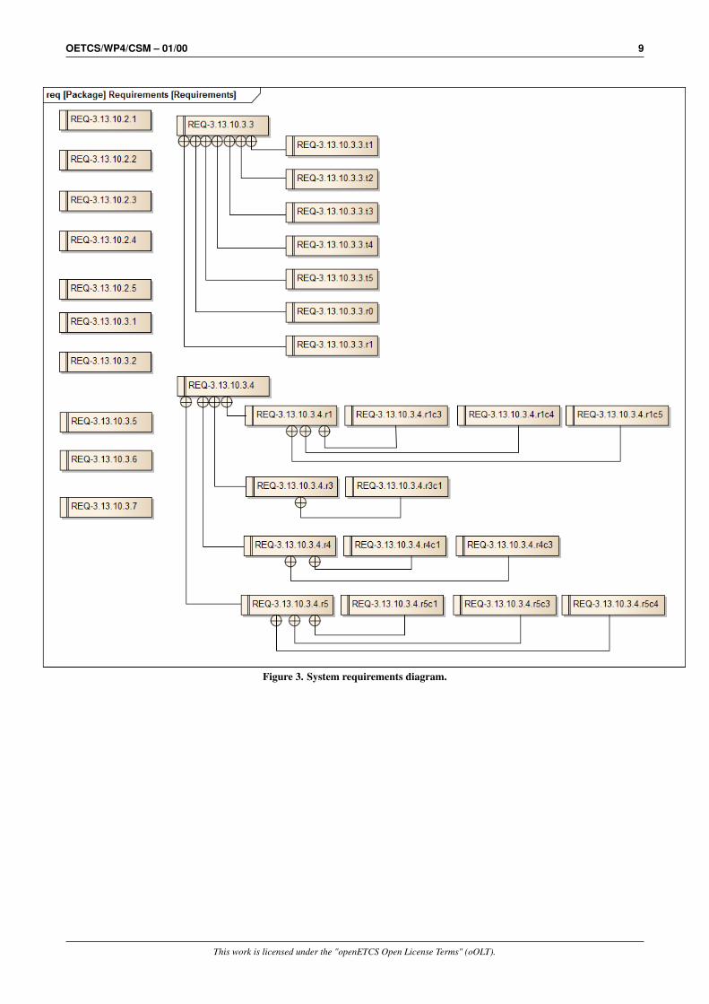
3.6 Requirements
Figure 3 shows the requirements reflected by the model. The requirement labels refer to thesections of the ETCS standard document [28], from where they have been imported into the model.To make this technical report sufficiently self-contained, we list the requirements applicable toCSM in Table 1, and adapt the wording and the cross references to the technical report.
In requirement REQ-3.13.10.2.2, the traction cut-off command on the train interface is notexplicitly addressed in our model, because it will always be triggered in synchrony with a brakingcommand. We assume the existence of a driver software layer in the EVC that automaticallytriggers traction cut-off if
• a traction cut-off interface is implemented for the EVC, and
• a service brake or emergency brake command is issued.
Requirement REQ-3.13.10.2.3 states that national values can only influence the usage of theservice brake when in TSM. We will therefore assume that the availability of the service brakeand its use for slowing down the train when the emergency braking condition is not yet fulfilledis constant (i.e., SBAvailable = 0 or SBAvailable = 1) during CSM operation.
Requirement REQ-3.13.10.3.3 is described by two tables (see Table 2 and Table 3 below), it isthen decomposed into sub-requirements REQ-3.13.10.3.3.t1, . . . , REQ-3.13.10.3.3.r1, each ofthem representing one line of these two tables.
Requirement REQ-3.13.10.3.4 is represented as a transition table, it is decomposed into sub-requirements, one for each relevant cells of the table (see Table 4).
Requirement REQ-3.13.10.3.7 is “delegated” to the surrounding software of the CSM: it isassumed in our model that the input VMRSP is always set by the CSM software environment in away that takes into account the min safe front end of the train.
3.7 Behavioural Specification
The behaviour of the ceiling speed monitor is modelled by the hierarchic state machine that isassociated with the SUT block of Fig. 2 and displayed in Fig. 4 (top-level state machine) andFig. 5 (lower-level state machine associated with composite state CSM_ON.
The top-level state machine controls activation and de-activation of the CSM. As soon as inputvariable csmSwitch on interface SnDMonitorIn gets value 1, the CSM is activated, and it isde-activated when csmSwitch falls back to 0. On activation, the auxiliary variable sbiCmdis set to EMER_BRAKE_CMD, if the input variable SBAvailable carries value 0, indicating
This work is licensed under the "openETCS Open License Terms" (oOLT).
OETCS/WP4/CSM – 01/00 9
Figure 3. System requirements diagram.
This work is licensed under the "openETCS Open License Terms" (oOLT).
OETCS/WP4/CSM – 01/00 10
Table 1. Requirements for the ceiling speed monitoring function.
id Description
REQ-3.13.10.2.1 The train speed indicated to the driver shall be identical to the speed used for the speed monitoring (i.e.the estimated speed Vest).
REQ-3.13.10.2.2 Once a Train Interface command (traction cut-off, service brake or emergency brake) is triggered, theon-board shall apply it until its corresponding revocation condition is met.
REQ-3.13.10.2.3 If there is no on-board interface with the service brake or if the use of the service brake command is notallowed by a National Value (only in Target speed monitoring),whenever a service brake command isspecified, the emergency brake command shall be triggered instead.
REQ-3.13.10.2.4 The emergency brake command, which is triggered instead of the service brake command when an SBIsupervision limit is exceeded, shall be revoked according to the requirements specified for the revocationof service brake command, unless the emergency brake command has been also triggered due to an EBIsupervision limit. In such case, the condition for revoking the emergency brake command due to EBIsupervision limit shall prevail.
REQ-3.13.10.2.5 The on-board shall revoke the Intervention status only when no brake command is applied by the speedand distance monitoring function.
REQ-3.13.10.3.1 The on-board equipment shall display the permitted speed (VMRSP).
REQ-3.13.10.3.2 When the supervision status is Overspeed, Warning or Intervention, the on-board equipment shall displaythe SBI speed (i.e. the FLOI speed; FLOI = First Line of Intervention).
REQ-3.13.10.3.3 The on-board shall compare the estimated speed with the ceiling supervision limits defined in [28,3.13.9.2] and shall trigger/revoke commands to the train interface (service brake if implemented oremergency brake) and supervision statuses as described in Table 2 (from [28, Table 5]) and Table 3(from [28, Table 6]).
REQ-3.13.10.3.4 The on-board equipment shall execute the transitions between the different supervision statuses asdescribed in Table 4 (see [28, 4.6.1] for details about the symbols). This table takes into account theorder of precedence between the supervision statuses and the possible updates of the MRSP while inceiling speed monitoring (e.g. when a TSR is revoked; TSR = Temporary Speed Restriction).
REQ-3.13.10.3.5 When the speed and distance monitoring function becomes active and the ceiling speed monitoring is thefirst one entered, the triggering condition t1 defined in Table 2 shall be checked in order to determinewhether the Normal status applies. If it is not the case, the on-board shall immediately set the supervisionstatus to the relevant value, applying a transition from the Normal status according to Table 4.
REQ-3.13.10.3.6 The Indication status is not used in ceiling speed monitoring. However, in case the ceiling speedmonitoring is entered and the supervision status was previously set to Indication, the on-board equipmentshall immediately execute one of the transitions from the Indication status, as described in Table 4.
REQ-3.13.10.3.7 The locations corresponding to a speed increase of the MRSP shall be supervised by the on-boardequipment taking into account the min safe front end of the train.
Table 2. Triggering of Train Interface commands and supervision statuses in ceiling speed monitoring(from [28, Table 5]).
id TC Estimated speed TI SSE
REQ-3.13.10.3.3.t1 t1 Vest ≤ VMRSP — Normal Status
REQ-3.13.10.3.3.t2 t2 Vest > VMRSP — Overspeed Status
REQ-3.13.10.3.3.t3 t3 Vest > VMRSP + dVwarning — Warning Status
REQ-3.13.10.3.3.t4 t4 Vest > VMRSP + dVsbi SB Intervention Status
REQ-3.13.10.3.3.t5 t5 Vest > VMRSP + dVebi EB Intervention Status
TC: trigger conditionTI: command triggered on train interface to brakesSB: trigger service brake command (if available, otherwise trigger emergency brake)EB: trigger emergency brake command SSE: supervision status entered
This work is licensed under the "openETCS Open License Terms" (oOLT).

OETCS/WP4/CSM – 01/00 11
Table 3. Revocation of Train Interface commands and supervision statuses in ceiling speed monitoring(from [28, Table 6]).
id RC Estimated Speed TICR SSR
REQ-3.13.10.3.3.r0 r0 Standstill EB Intervention Status
REQ-3.13.10.3.3.r1 r1 Vest ≤ VMRSP SB, EBa Indication StatusOverspeed StatusWarning StatusIntervention Status (if SBI)Intervention Status (if EB andallowRevokeEB = 1)
aOnly if allowRevokeEB = 1.
RC: revocation conditionTICR: command revoked on train interface to brakesSSR: supervision status revoked
Table 4. Transitions between supervision statuses in ceiling speed monitoring (from [28, Table 7]).
Normal Status < r1 < r1 < r1 < r0, r1
Indication Status
t2 > t2 > Overspeed Status
t3 > t3 > t3 > Warning Status
t4, t5 > t4, t5 > t4, t5 > t4, t5 > Intervention Status
The sub-requirements IDs associated with each cell in the transition table are of the formREQ-3.13.10.3.4.rX.cY where X and Y are the row and column indexes, respectively.
Figure 4. Ceiling speed monitoring – top-level state machine.
This work is licensed under the "openETCS Open License Terms" (oOLT).

OETCS/WP4/CSM – 01/00 12
Figure 5. Ceiling speed monitoring state machine.
This work is licensed under the "openETCS Open License Terms" (oOLT).

OETCS/WP4/CSM – 01/00 13
that no separate service brake can be used for slowing down the train, so that the emergencybrake has to be used for this purpose. Conversely, when SBAvailable = 1, sbiCmd is set toSERVICE_BRAKE_CMD.
While in composite state CSM_ON, do actions are executed as specified by operationscalc_permitted_speed_to_driver(), calc_speed_onboard(), and calc_speed_to_driver() introducedabove. The effect of these do actions is that variables permittedSpeedToDriver, speedOnBoard,and speedToDriver are set consistently to the current values depending on Vest and VMRSP, respec-tively, as described above. The do-actions are executed whenever all state machine transitionsare blocked, and the value of the left-hand side variable of the assignment performed by one ofthese operations differs from the valuation of the right-hand side expression. As a consequence,the necessary updates of these three output variables are executed in zero time after any inputchange.
Subordinate state machine CSM_ON specifies the detailed behaviour of the CSM. Its executionstarts in basic state NORMAL, where the ‘NORMAL’ indication is displayed on the DMI andbrakes are released (TICmd = NO_CMD). When the speed increases above the maximalspeed allowed (Vest > VMRSP), the state machine transits to basic state OVERSPEED, wherethe ‘OVERSPEED’ indication is displayed to the train engine driver. If the train continuesoverspeeding until the warning threshold VMRSP + dVwarning(VMRSP) is exceeded, a transition intothe WARNING state is performed, accompanied by an indication change on the DMI. Acceleratingfurther until Vest > VMRSP+dVsbi(VMRSP) leads to a transition into basic state SERVICE_BRAKE,where either the service brake or the emergency brake is triggered, depending on the value storedbefore in variable sbiCmd. The DMI display changes to ‘INTERVENTION’.
The intervention status is realised by two basic state machine states, SERVICE_BRAKE andEMER_BRAKE. From SERVICE_BRAKE it is still possible to return to NORMAL, as soonas the speed has been decreased below the overspeeding threshold. When the train, however,continues its acceleration until the emergency braking threshold has been exceeded (Vest >
VMRSP + dVebi(VMRSP)), basic state EMER_BRAKE is entered. From there, a state machinetransition to NORMAL is only possible if the train comes to a standstill, or if the nationalregulations (variable allowRevokeEB) allow to release the brakes as soon as overspeeding hasstopped.
Observe that the run-to-completion semantics of state machines also allows for zero-time transi-tions from, for example, NORMAL to EMER_BRAKE. If, while in basic state NORMAL, theinputs change such that Vest > VMRSP + dVebi(VMRSP) becomes true1, the state machine transitionfrom NORMAL to OVERSPEED leads to a transient model state, because guard conditionVest > VMRSP +dVwarning(VMRSP) is already fulfilled, and the state machine transits to WARNING.Similarly, guards Vest > VMRSP + dVsbi(VMRSP) and Vest > VMRSP + dVebi(VMRSP) also evaluateto true, so that the next quiescent state is reached in basic state EMER_BRAKE. ThereforeREQ-3.13.10.3.4.r5c1 which requires direct transitions from Normal status to Intervention statusis fulfilled by the CSM_ON state machine: if the guard conditions have the appropriate valu-ations, the required target states can be reached in zero time, that is, in one observable EVCprocessing cycle. Analogously, the state machine fulfils requirements REQ-3.13.10.3.4.r5c2,REQ-3.13.10.3.4.r5c3, REQ-3.13.10.3.4.r4c1 without needing direct state machine transitionarrows between the respective state machine states.
1This would be an exceptional behaviour situation, caused, for example, by temporary unavailability of odometrydata, so that a “sudden jump” of Vest would be observed by the CSM.
This work is licensed under the "openETCS Open License Terms" (oOLT).

OETCS/WP4/CSM – 01/00 14
3.8 Requirements Tracing
SysML provides language elements for relating model elements to requirements, using the «sat-isfy» relationship from model elements to requirements symbols in arbitrary SysML diagrams [21,Section 16]. Exploiting this language feature supports
• model validation, and
• requirements-based testing.
In the former case, missing requirements can be detected if they cannot be linked to structural orbehavioural model elements in the appropriate way. In latter case, execution traces through themodel covering a given structural or behavioural model element represent test cases contributingto the verification of all requirements related to the model element under consideration.
Tables 5 associates the SysML elements with the requirements they satisfied. “Submachine State”and “Atomic State” are the top-level and state machine states, respectively. The “Constraints" arethe LTL formulas used to relate the most complex requirements to execution traces as explainedin the following paragraphs.
The complexity of «satisfy» relations between structural or behavioural model elements dependson the complexity of the requirement and the way each requirement is reflected by the structuraland behavioural model. Consider, for example (see Table 1), requirement
REQ-3.13.10.2.1: The train speed indicated to the driver shall be identical to the speedused for the speed monitoring (i.e. the estimated speed Vest).
Every model trace where the CSM is activated is suitable for verifying this requirement,because the DMI variable speedToDriver is updated by the actual speed Vest via operationcalc_speed_to_driver(), whenever the ceiling speed monitor is active, that is, in composite stateCSM_ON. Therefore CSM_ON is linked to REQ-3.13.10.2.1 by the «satisfy» relation, asexpressed in Table 5, row 1.
SysML also allows to express traceability relationships in a graphical way, by drawing arrowsfrom model elements to requirements as shown in Fig. 6. This technique, however, tends toclutter structural and behavioural diagrams as soon as more than a few requirements are involved.Therefore the tabular notation in Table 5 is preferable and supported by most state-of-the-artSysML modelling tools.
A more complex case of requirements tracing presents itself if one or more transitions are relatedto a given requirement. This is the case for the requirement
REQ-3.13.10.2.2: Once a Train Interface command (traction cut-off, service brakeor emergency brake) is triggered, the on-board shall apply it until its correspondingrevocation condition is met.
As modelled in Fig. 5, we have two revocation conditions; one is reflected by the transitionfrom basic state SERVICE_BRAKE to NORMAL, the other from EMER_BRAKE to NORMAL.Therefore both transitions are related to REQ-3.13.10.2.2, as specified in row 2 of Table 5.
This work is licensed under the "openETCS Open License Terms" (oOLT).
OETCS/WP4/CSM – 01/00 15
Table 5. Requirements links to the SysML Elements
No. Requirement ←− «satisfy»
1 REQ-3.13.10.2.1 «Composite State» CSM_ON
2 REQ-3.13.10.2.2 «Transition» [EMER_BRAKE - NORMAL]
«Transition» [SERVICE_BRAKE - NORMAL]
3 REQ-3.13.10.2.3 «Transition» [CSM_OFF - CSM_ON]
«Basic State» SERVICE_BRAKE
«Constraint» constraint_03
4 REQ-3.13.10.2.4 «Constraint» constraint_02
«Transition» [EMER_BRAKE - NORMAL]
«Constraint» constraint_01
5 REQ-3.13.10.2.5 «Transition» [EMER_BRAKE - NORMAL]
«Transition» [SERVICE_BRAKE - NORMAL]
6 REQ-3.13.10.3.1 «Submachine State» CSM_ON
7 REQ-3.13.10.3.2 «Basic State» OVERSPEED
«Basic State» SERVICE_BRAKE
«Basic State» WARNING
«Basic State» EMER_BRAKE
8 REQ-3.13.10.3.3.r0 «Transition» [EMER_BRAKE - NORMAL]
9 REQ-3.13.10.3.3.r1 «Transition» [OVERSPEED - NORMAL]
«Transition» [SERVICE_BRAKE - NORMAL]
«Transition» [WARNING - NORMAL]
«Transition» [EMER_BRAKE - NORMAL]
10 REQ-3.13.10.3.3.t1 «Basic State» NORMAL
11 REQ-3.13.10.3.3.t2 «Basic State» OVERSPEED
12 REQ-3.13.10.3.3.t3 «Basic State» WARNING
13 REQ-3.13.10.3.3.t4 «Basic State» SERVICE_BRAKE
14 REQ-3.13.10.3.3.t5 «Basic State» EMER_BRAKE
15 REQ-3.13.10.3.4.r1c3 «Transition» [OVERSPEED - NORMAL]
16 REQ-3.13.10.3.4.r1c4 «Transition» [WARNING - NORMAL]
17 REQ-3.13.10.3.4.r1c5 «Transition» [EMER_BRAKE - NORMAL]
«Transition» [SERVICE_BRAKE - NORMAL]
18 REQ-3.13.10.3.4.r3c1 «Transition» [NORMAL - OVERSPEED]
19 REQ-3.13.10.3.4.r4c1 «Constraint» constraint_08
20 REQ-3.13.10.3.4.r4c3 «Transition» [OVERSPEED - WARNING]
21 REQ-3.13.10.3.4.r5c1 «Constraint» constraint_10
«Constraint» constraint_09
22 REQ-3.13.10.3.4.r5c3 «Constraint» constraint_12
«Constraint» constraint_11
23 REQ-3.13.10.3.4.r5c4 «Transition» [WARNING - SERVICE_BRAKE]
«Transition» [SERVICE_BRAKE - EMER_BRAKE]
«Constraint» constraint_13
24 REQ-3.13.10.3.5 «Constraint» constraint_05
«Constraint» constraint_06
«Constraint» constraint_07
«Basic State» NORMAL
«Constraint» constraint_04
25 REQ-3.13.10.3.6 «Constraint» constraint_05
«Constraint» constraint_06
«Constraint» constraint_07
«Constraint» constraint_04
The constraints constraint_01,. . . ,constraint_13 are specified in Table 6.
This work is licensed under the "openETCS Open License Terms" (oOLT).

OETCS/WP4/CSM – 01/00 16
Figure 6. Graphical representation of the «satisfy» relation in a state machine diagram.
In the most complex case we have to handle situations where requirements are reflected by tracesvisiting model state vectors2 fulfilling certain constraints, and these model state vectors have tobe visited by the traces in a specific order. Such a situation is reflected, for example, by
REQ-3.13.10.3.4: The on-board equipment shall execute the transitions between thedifferent supervision statuses as described in Table 4 (see [28, 4.6.1] for details about thesymbols). This table takes into account the order of precedence between the supervisionstatuses and the possible updates of the MRSP while in ceiling speed monitoring (e.g.when a TSR is revoked; TSR = Temporary Speed Restriction).
This requirement has been decomposed into atomic sub-requirements REQ-3.13.10.3.4.r1c3, . . . ,REQ-3.13.10.3.4.r5c4, as explained in Section 3.6. Some of these sub-requirements are againreflected by transitions, as specified in rows 15, 16, 17, 18, and 20 of Table 5. RequirementREQ-3.13.10.3.4.r5c1, however, specifies the possibility to directly transit from NORMAL toSERVICE_BRAKE or EMER_BRAKE. This cannot be specified by simply linking a behaviouralmodel element to the requirement, because we have avoided to draw direct state machinetransitions from NORMAL to SERVICE_BRAKE or EMER_BRAKE, since those transitionsare implicitly realised by the run-to-completion semantics, as explained above. Consider, forexample, the zero-time transition NORMAL −→ SERVICE_BRAKE. To cover this situation, weneed to
1. Enter NORMAL in a quiescent model state – this is specified by
[NORMAL ∧ Vest ≤ VMRSP]
2. Stay there until the speed exceeds VMRSP + dVsbi(VMRSP) but remains less or equal to VMRSP +
dVebi.2A model state vector consists of valuations of inputs, outputs, and internal model variables, as well as of variable
valuations indicating the basic state machine states currently active.
This work is licensed under the "openETCS Open License Terms" (oOLT).
OETCS/WP4/CSM – 01/00 17
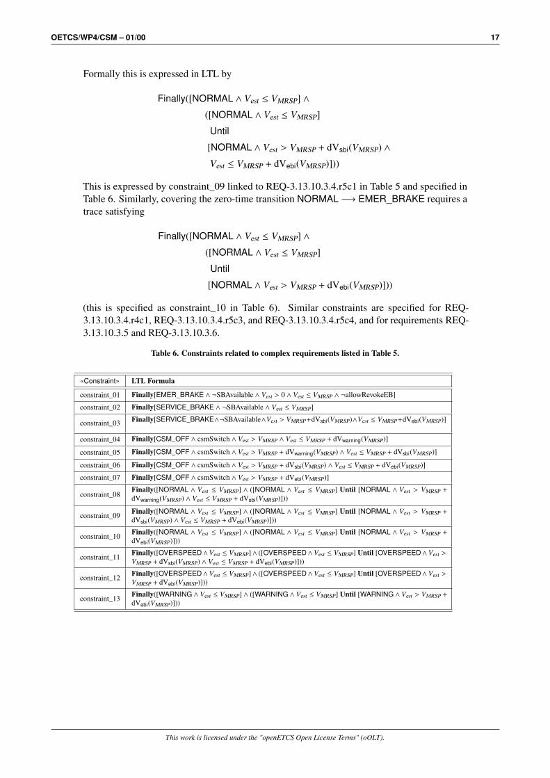
Formally this is expressed in LTL by
Finally([NORMAL ∧ Vest ≤ VMRSP] ∧
([NORMAL ∧ Vest ≤ VMRSP]
Until
[NORMAL ∧ Vest > VMRSP + dVsbi(VMRSP) ∧
Vest ≤ VMRSP + dVebi(VMRSP)]))
This is expressed by constraint_09 linked to REQ-3.13.10.3.4.r5c1 in Table 5 and specified inTable 6. Similarly, covering the zero-time transition NORMAL −→ EMER_BRAKE requires atrace satisfying
Finally([NORMAL ∧ Vest ≤ VMRSP] ∧
([NORMAL ∧ Vest ≤ VMRSP]
Until
[NORMAL ∧ Vest > VMRSP + dVebi(VMRSP)]))
(this is specified as constraint_10 in Table 6). Similar constraints are specified for REQ-3.13.10.3.4.r4c1, REQ-3.13.10.3.4.r5c3, and REQ-3.13.10.3.4.r5c4, and for requirements REQ-3.13.10.3.5 and REQ-3.13.10.3.6.
Table 6. Constraints related to complex requirements listed in Table 5.
«Constraint» LTL Formula
constraint_01 Finally[EMER_BRAKE ∧ ¬SBAvailable ∧ Vest > 0 ∧ Vest ≤ VMRSP ∧ ¬allowRevokeEB]
constraint_02 Finally[SERVICE_BRAKE ∧ ¬SBAvailable ∧ Vest ≤ VMRSP]
constraint_03 Finally[SERVICE_BRAKE∧¬SBAvailable∧Vest > VMRSP+dVsbi(VMRSP)∧Vest ≤ VMRSP+dVebi(VMRSP)]
constraint_04 Finally[CSM_OFF ∧ csmSwitch ∧ Vest > VMRSP ∧ Vest ≤ VMRSP + dVwarning(VMRSP)]
constraint_05 Finally[CSM_OFF ∧ csmSwitch ∧ Vest > VMRSP + dVwarning(VMRSP) ∧ Vest ≤ VMRSP + dVsbi(VMRSP)]
constraint_06 Finally[CSM_OFF ∧ csmSwitch ∧ Vest > VMRSP + dVsbi(VMRSP) ∧ Vest ≤ VMRSP + dVebi(VMRSP)]
constraint_07 Finally[CSM_OFF ∧ csmSwitch ∧ Vest > VMRSP + dVebi(VMRSP)]
constraint_08Finally([NORMAL ∧ Vest ≤ VMRSP] ∧ ([NORMAL ∧ Vest ≤ VMRSP] Until [NORMAL ∧ Vest > VMRSP +
dVwarning(VMRSP) ∧ Vest ≤ VMRSP + dVsbi(VMRSP)]))
constraint_09 Finally([NORMAL ∧ Vest ≤ VMRSP] ∧ ([NORMAL ∧ Vest ≤ VMRSP] Until [NORMAL ∧ Vest > VMRSP +
dVsbi(VMRSP) ∧ Vest ≤ VMRSP + dVebi(VMRSP)]))
constraint_10 Finally([NORMAL ∧ Vest ≤ VMRSP] ∧ ([NORMAL ∧ Vest ≤ VMRSP] Until [NORMAL ∧ Vest > VMRSP +
dVebi(VMRSP)]))
constraint_11 Finally([OVERSPEED∧Vest ≤ VMRSP]∧ ([OVERSPEED∧Vest ≤ VMRSP] Until [OVERSPEED∧Vest >VMRSP + dVsbi(VMRSP) ∧ Vest ≤ VMRSP + dVebi(VMRSP)]))
constraint_12 Finally([OVERSPEED∧Vest ≤ VMRSP]∧ ([OVERSPEED∧Vest ≤ VMRSP] Until [OVERSPEED∧Vest >VMRSP + dVebi(VMRSP)]))
constraint_13 Finally([WARNING ∧ Vest ≤ VMRSP] ∧ ([WARNING ∧ Vest ≤ VMRSP] Until [WARNING ∧ Vest > VMRSP +
dVebi(VMRSP)]))
This work is licensed under the "openETCS Open License Terms" (oOLT).
OETCS/WP4/CSM – 01/00 18
4 Formal Semantics – the Transition Relation
4.1 Semantic Definition Scope
In this section the formal behavioural semantics of the CSM model M written in SysML isspecified. The exposition is restricted to the situation where the CSM has already been switchedon; this scenario is completely captured by state machine CSM_ON depicted in Fig. 5. Thisrestriction is motivated by the fact that the activation/deactivation scenario for the CSM as shownin state machine CSM (Fig. 4) is incomplete without the models for TSM and RSM. These modelcomponents define the SUT behaviour when CSM is in state CSM_OFF.
4.2 State Transition System Semantics
The behaviour of the CSM SysML model M can be formalised by mapping M to a statetransition system (STS) S = (S , s0,R) with state space S , initial state s0 ∈ S and transitionrelation R ⊆ S × S . An infinite sequence π = s.s1.s2 . . . of S-states is called a computation or apath of S, if and only if it satisfies
s = s0 ∧ (∀i ∈ N : (si−1, si) ∈ R)
A finite computation prefix is called a trace.
The behavioural semantics of a SysML modelM is given by the set of computations that can beexecuted by the state transition system S associated withM.
4.3 State Space
For mappingM to S, we use state spaces over variable valuations: let V be a finite set of variablesymbols for variables v ∈ V with values in some domain D =
⋃v∈V Dv. The state space S of S is
the set of all variable valuations s : V → D with s(v) ∈ Dv. The variables of V are partitioned intoinput variables, internal model variables, and output variables; for the CSM model this results in
V = I ∪ M ∪ O
I = {Vest,VMRSP, allowRevokeEB}
M = {`, sbiCmd}
O = {DMICmd,TICmd}
These variables have domains as introduced in Section 3, but here we use integer values insteadof enumeration types. The enumeration to integer association is defined in Fig. 1.
DVest = DVMRSP = [0, 350]
DallowRevokeEB = DsbiCmd = D` = {0, 1}
DTICmd = {0, 1, 2}
DDMICmd = {0, 1, 2, 3, 4}
Internal variable ` does not occur in the SysML model described in Section 3; it is used hereto reduce the state space: each of the basic states NORMAL, OVERSPEED, WARNING, aswell as the intervention states of the state machine in Fig. 5 are associated with specific outputson DMICmd. Therefore all basic states of this machine are completely identified if we havea means to distinguish SERVICE_BRAKE from EMER_BRAKE in the case DMICmd = 4
This work is licensed under the "openETCS Open License Terms" (oOLT).

OETCS/WP4/CSM – 01/00 19
(INTERVENTION). To this end, auxiliary variable ` will be set to 1 if the state machine of Fig. 5resides in basic state SERVICE_BRAKE; otherwise ` will be set to 0. Using ` in this way allowsus to identify the basic states as specified in Table 7.
Table 7. Identification of basic states in machine CSM_ON
State Machine in Basic State Equivalent to
NORMAL DMICmd = 0
OVERSPEED DMICmd = 2
WARNING DMICmd = 3
SERVICE_BRAKE DMICmd = 4 ∧ ` = 1
EMER_BRAKE DMICmd = 4 ∧ ` = 0
We use a short-hand tuple notation for states: s = (d1, . . . , d7) with di ∈ D denotes the statesatisfying
s(Vest) = d1, s(VMRSP) = d2, s(allowRevokeEB) = d3,
s(`) = d4, s(sbiCmd) = d5,
s(DMICmd) = d6, s(TICmd) = d7
4.4 Quiescent and Transient States
The STS covered by our testing theory have state spaces that can be partitioned into disjoint setsS = S Q ∪ S T , where S Q denotes quiescent states and S T transient states. In quiescent states,the system is stable and cannot progress without a change of inputs. When these inputs change,internal states and outputs remain unchanged. Transitions emanating from quiescent states maylead to other quiescent states or to transient states. In contrast to this, each transient state hasexactly one post-state which is quiescent, and the transition to this post-state is immediate andmay change internal state variables and outputs only. The initial state s0 of the STS underconsideration is always quiescent.
From the intuitive interpretation of the CSM model, we see, for example, that the states si =
(Vest,VMRSP, allowRevokeEB, `, sbiCmd,DMICmd,TICmd),
s0 = (50, 100, 0, 0, 1, 0, 0)
s1 = (100.1, 100, 0, 1, 1, 4, 1)
s2 = (50, 100, 0, 0, 1, 4, 2)
are quiescent, while the states
s3 = (100.7, 100, 0, 0, 1, 0, 0)
s4 = (99.8, 100, 0, 1, 1, 4, 1)
s5 = (0, 100, 0, 0, 1, 4, 2)
are transient.
4.5 Initial State
This work is licensed under the "openETCS Open License Terms" (oOLT).

OETCS/WP4/CSM – 01/00 20
The initial state corresponds to the CSM in its de-activated state. We associate the deactivationstate with encoding
s0 = (0, 0, 0, 0, 0, 0, 0)
and the first input change activates the CSM.
The existence of a service brake (sbiCmd = 1) is a configuration parameter of the train hardware.Therefore it cannot be regarded as an input to the CSM that may change arbitrarily during itsexecution, but as a constant value sbiCmd = sb0 ∈ {0, 1} that remains invariant during each testexecution.
4.6 Transition Relation – General Construction Rules
The transition relation R ⊆ S ×S specifying the possible state changes of the STS associated withthe CSM is infinite, since the input domains are infinite. The transition relation, however, can berepresented by means of a finite predicate R relating pre-states to post-states. R is a propositionwith free variables in V and V ′ = {v′ | v ∈ V}, the primed variable symbols denoting post-states.The transition relation is specified by R via
R = {(s0, s1) ∈ S × S | R[s0(v)/v, s1(v)/v′ | v ∈ V]}
Predicate R[s0(v)/v, s1(v)/v′ | v ∈ V] results from R by replacing every unprimed variable v ∈ Voccurring in R by its pre-state value s0(v), and every primed variable v′ ∈ V ′ by its post-statevalue s1(v).
The propositional representation of the transition relation is crucial for automated test datageneration: as explained in [23], concrete test data is calculated by means of constraint solvingtechniques applied to formulas of the type
tc ≡ J(s0) ∧n∧
i=1
R(si−1, si) ∧G(s0, . . . , sn)
where G(s0, . . . , sn+1) encodes a test objective and∧n
i=1 R(si−1, si) asserts that every solution isa trace of the model. Each R(si−1, si) is represented by means of R as a proposition where newinputs to be selected in quiescent state si can be freely chosen by the solver, but their effect oninternal model variables and outputs is determined by R. Thus we are interested in propositionalrepresentations R mainly for the purpose of tool construction.
While R is not uniquely determined in the general case, well-defined construction rules areimplied by [12], if R is to be applied for the purpose of equivalence class construction.
1. The canonic structure of R is
R ≡
k∨i=0
(ϕi(V) ∧ ψi(V,V ′)
)where ϕi(V) is a proposition with free variables in V only, and ψi(V,V ′) has free variables inV and V ′. ϕi(V) describes the precondition for a transition to fire, and ψi(V,V ′) specifies thetransition’s effect.
2. Each ϕi(V) specifies a set of reachable quiescent states, or a set of reachable transient states.
This work is licensed under the "openETCS Open License Terms" (oOLT).

OETCS/WP4/CSM – 01/00 21
3. All atomic propositions occurring in R and involving primed or unprimed internal statevariables or output variables v, v′, v ∈ M ∪ O, must be of the form
v = d or v′ = d, with d ∈ Dv
Recall that the domains of internal state and outputs variables are finite, therefore the numberof atomic propositions v = d is finite. Moreover, every atomic proposition involving variablesfrom I and M∪O can be transformed into a disjunction of conjunctions of atomic propositionsp with free variables from either I or M ∪ O only3.
4. For transitions emanating from quiescent states, ϕi(V) is constructed according to the rules
• Every state s satisfying ϕi(V) must be reachable and quiescent.
• For any reachable quiescent state s there is a unique ϕi(V) such that s satisfies ϕi(V).
• Every state s satisfying ϕi(V) has the same valuation of internal state and outputvariables.
• For any reachable quiescent states s and r with the same valuation of internal state andoutput variables, s and r satisfy the same ϕi(V).
Again, since the domains of internal state and outputs variables are finite, this constructionrule leads to a finite number of propositions ϕi(V). We assume that propositions ϕi(V), i =
0, . . . , k0 − 1 specify quiescent states.
5. For transitions emanating from transient states, ϕi(V) is constructed according to the rules
• Every state s satisfying ϕi(V) must be reachable and transient.
• For any transient state s there is a unique ϕi(V) such that s satisfies ϕi(V).
• There exists an index j, such that ϕ j(V) specifies a set of quiescent states according toRule 3, and every state s satisfying ϕi(V) has a post-state satisfying ϕ j(V).
• For any transient states s and r with post-states satisfying the same ϕ j(V), s and r satisfythe same ϕi(V).
We assume that ϕk0+i(V), i = 0, . . . ,≤ k0−1 specify transient states. By construction of ϕi(V) andϕk0+i(V), the number of propositions specifying quiescent states according to Rule 4 is greaterthan or equals the number of transient-state propositions built according to Rule 5. This is easy tosee, because each transient state s satisfying ϕk0+i(V) has a post-state satisfying the same ϕ j(V),and this ϕ j(V) is unique. If the number of quiescent ϕi(V) is grater than the number of transientϕk0+i(V), then there are some reachable quiescent states which do not have any transient pre-states.This may only occur for the quiescent state s0. As a consequence we can assume that propositionϕ0(V) specifies the quiescent initial state, and the propositions ϕk(V), k > 0, are ordered in such away that the quiescent post-states visited from transient states satisfying ϕk0+i(V) are all specifiedby ϕi(V). The existence of ϕk0(V) depends on whether there is a transition from transient statesto s0 or if the initial state is never re-visited.
In the case of quiescent pre-states, ψi(V,V ′) is always the same proposition qpsc(V,V ′), where“qpsc” stands for quiescent post-state condition.
qpsc(V,V ′) ≡
∨x∈I
x′ , x
∧ ∧v∈M∪O
v′ = v
3Consider, for example, atomic proposition x < m with Dx = R and Dm = {0, 1}. Then x < m ≡ (x < 0 ∧ m =
0) ∨ (x < 1 ∧ m = 1).
This work is licensed under the "openETCS Open License Terms" (oOLT).

OETCS/WP4/CSM – 01/00 22
This specifies that at least one input variable must change its value during a transition from aquiescent state, and all internal state and output valuations remain unchanged.
Transitions from transient states to quiescent states always leave inputs unchanged; this leads tothe complementary transient post-state condition
tpsc(V,V ′) ≡∧v∈I
v′ = v
so the effect of the transition from transient pre-state to quiescent post-state can be written as
ψk0+i(V,V ′) ≡ ψk0+i(V,V′) ∧ tpsc(V,V ′)
where ψk0+i(V,V′) is still to be determined.
As a consequence of Rule 4, every ϕi(V) characterising a subset of quiescent states is of the form
ϕi(V) ≡ ϕIi (I) ∧ ξi(M ∪ O) (5)
ξi(M ∪ O) ≡∧m∈M
(m = dmi ) ∧
∧y∈O
(y = dyi ), dm
i ∈ Dm, dyi ∈ Dy (6)
so that ϕIi (I) is a (generally non-atomic) proposition over free variables from I.
As a consequence of Rule 5 and of our numbering conventions, each ϕk0+i(V) characterising asubset of transient states satisfies
∀s1, s2 ∈ S : s1(ϕk0+i) ∧ R(s1, s2)⇒ s2(ϕi)
This means that ϕk0+i(V) is constructed for transient states in such a way that all post-states ofthe transient state set
Bi = {s ∈ S | s(ϕk0+i(V))}
are members of the same setAi = {s ∈ S | s(ϕi(V))}
of quiescent states. Therefore each ψk0+i(V,V ′) specifying the effect of a transition from transientto quiescent state can be structured as
ψk0+i(V,V ′) ≡ ξi[m′/m, y′/y | m ∈ M, y ∈ O] ∧ tpsc(V,V ′)
where ξi[m′/m, y′/y | m ∈ m, y ∈ O] is the proposition specifying internal state and output valuesfor the associated set Ai of quiescent states, but each internal model state variable m and eachoutput variable y are replaced by their primed versions m′ and y′, respectively. Conversely, ifBi can be reached from quiescent state set Ak by means of input changes satisfying a certainproposition ϕI
k,i, these reachable elements s ∈ Bi satisfy ϕIk,i ∧ ξk, since internal state values and
outputs do not change when transiting from an Ak-state to a Bi-state. As a consequence, theproposition ϕk0+i(V) characterising Bi-states has a canonic structure
ϕk0+i(V) ≡k0−1∨q=0
(ϕI
q,i(V) ∧ ξq(V))
(7)
where ϕIq,i(V) ≡ false, if there are no transitions from Aq-states to Bi-states.
This work is licensed under the "openETCS Open License Terms" (oOLT).

OETCS/WP4/CSM – 01/00 23
Summarising, the systems covered by our equivalence class testing theory have a behaviouralsemantics that can be expressed by an associated STS whose transition relation can be specifiedby means of a proposition
R(V,V ′) ≡k0−1∨i=0
(ϕI
i (I) ∧ ξi(M ∪ O) ∧ qpsc(V,V ′))∨ (8)
k0−1∨i=0
((k0−1∨q=0
ϕIq,i(I) ∧ ξq(M ∪ O)) ∧ (9)
ξi[m′/m, y′, y | m ∈ M, y ∈ O] ∧ tpsc(V,V ′))
(10)
where k0 + 1 is the number of reachable quiescent state classes Ai, each determined by a specificvaluation of internal states and outputs, as specified by ξi.
4.7 Transition Relation for the CSM
With the preparations of the previous section at hand, we are now in the position to specify theproposition R for the ceiling speed monitor, as applicable to all states of S that are reachablefrom initial state s0. To this end, the propositions occurring in the canonic representation shownin Equation (8) are specified one by one.
4.7.1 Propositions Specifying Internal State and Outputs – ξi.
The following combinations of internal state values and output values are reachable; this resultsin k0 = 5 and in the following propositions.
ξ0(V) ≡ ` = 0 ∧ DMICmd = 0 ∧ TICmd = 0
ξ1(V) ≡ ` = 0 ∧ DMICmd = 2 ∧ TICmd = 0
ξ2(V) ≡ ` = 0 ∧ DMICmd = 3 ∧ TICmd = 0
ξ3(V) ≡ ` = 1 ∧ DMICmd = 4 ∧ TICmd = 2 − sb0
ξ4(V) ≡ ` = 0 ∧ DMICmd = 4 ∧ TICmd = 2
4.7.2 Propositions Specifying Input Conditions for Quiescent Classes – ϕIi .
The input conditions for the 5 quiescent class A0, . . . , A4 – each class Ai associated with internalstate and output valuation ξi – are defined as follows.
ϕI0(V) ≡ Vest ≤ VMRSP (11)
ϕI1(V) ≡ VMRSP < Vest ∧ Vest ≤ VMRSP + dVwarning(VMRSP) (12)
ϕI2(V) ≡ VMRSP < Vest ∧ Vest ≤ VMRSP + dVsbi(VMRSP) (13)
ϕI3(V) ≡ VMRSP < Vest ∧ Vest ≤ VMRSP + dVebi(VMRSP) (14)
ϕI4(V) ≡ (0 < Vest ∧ allowRevokeEB = 0) ∨ (VMRSP < Vest ∧ allowRevokeEB = 1) (15)
The propositions ϕIi (V), ξi(V) cover the following quiescent state classes.
ϕI0(V) ∧ ξ0(V) specifies the quiescent states associated with basic state NORMAL, while the train
speed does not exceed VMRSP.
ϕI1(V) ∧ ξ1(V) specifies the quiescent states associated with basic state OVERSPEED, while the
train speed does not exceed the boundary for transiting to the WARNING state, and the speedhas not yet been reduced enough to transit back to NORMAL.
This work is licensed under the "openETCS Open License Terms" (oOLT).

OETCS/WP4/CSM – 01/00 24
ϕI2(V) ∧ ξ2(V) specifies the quiescent states associated with basic state WARNING, while the
train speed does not exceed the boundary for transiting to the SERVICE_BRAKE state, andthe speed has not yet been reduced enough to transit back to NORMAL.
ϕI3(V) ∧ ξ3(V) specifies the quiescent states associated with basic state SERVICE_BRAKE,
while the train speed does not exceed the boundary for transiting to the EMER_BRAKEstate, and the speed has not yet been reduced enough to transit back to NORMAL. Outputspecification TICmd = 2−sb0 which is part of ξ3(V) requires that the service brake is triggered(TICmd = 1) if such a brake is available (constant sb0 = 1); otherwise the emergency brakeis triggered (TICmd = 2).
ϕI4(V) ∧ ξ4(V) specifies the quiescent states associated with basic state
EMER_BRAKE, while either
• the speed Vest is still greater zero and input allowRevokeEB = 0 forbids to return toNORMAL before the train has come to a standstill, or
• the CSM may return to NORMAL as soon as Vest ≤ VMRSP because allowRevokeEB = 1,but currently the estimated speed is still greater than VMRSP.
For building more fine-grained equivalence classes (see Section 5 below) it is important toobserve that the functions dVwarning(VMRSP), dVsbi(VMRSP), dVebi(VMRSP) contain internal casedistinctions as specified in Equations (2 — 4). Inserting these case distinctions into the inequalitiesreferencing these functions in propositions ϕI
i (V), i = 1, 2, 3 results in refined predicates
ϕI1(V) ≡ (VMRSP ≤ 110 ∧ VMRSP < Vest ≤ VMRSP + 4) ∨ (16)
(110 < VMRSP ≤ 140 ∧ VMRSP < Vest ≤3130
VMRSP +13
) ∨ (17)
(140 < VMRSP ∧ VMRSP < Vest ≤ VMRSP + 5) (18)
ϕI2(V) ≡ (VMRSP ≤ 110 ∧ VMRSP < Vest ≤ VMRSP + 5.5) ∨ (19)
(110 < VMRSP ≤ 210 ∧ VMRSP < Vest ≤209200
VMRSP +55
100) ∨ (20)
(210 < VMRSP ∧ VMRSP < Vest ≤ VMRSP + 10) (21)
ϕI3(V) ≡ (VMRSP ≤ 110 ∧ VMRSP < Vest ≤ VMRSP + 7.5) ∨ (22)
(110 < VMRSP ≤ 210 ∧ VMRSP < Vest ≤4340
VMRSP −34
) ∨ (23)
(210 < VMRSP ∧ VMRSP < Vest ≤ VMRSP + 15) (24)
4.7.3 Quiescent Post-State Condition – qpsc.
For the CSM, this conditions is defined as follows.
qpsc ≡ (Vest′,VMRSP
′, allowRevokeEB′) , (Vest,VMRSP, allowRevokeEB) ∧
`′ = ` ∧ DMICmd′ = DMICmd ∧ TICmd′ = TICmd ∧ sbiCmd′ = sb0
4.7.4 Transient Post-State Condition – tpsc.
For the CSM, this conditions is defined as follows.
tpsc ≡ Vest′ = Vest ∧ VMRSP
′ = VMRSP ∧ allowRevokeEB′ = allowRevokeEB ∧
sbiCmd′ = sb0
4.7.5 Transient State Input Conditions – ϕIq,i.
As explained in the previous section, the transient states of some class Bi are characterised bydisjunctions of predicates ϕI
q,i(V) ∧ ξq(V), where ϕIq,i denotes the condition on input changes
This work is licensed under the "openETCS Open License Terms" (oOLT).
OETCS/WP4/CSM – 01/00 25
required to reach Bi states from Aq states. These propositions are specified as follows.
ϕI0,1(V) ≡ VMRSP < Vest ∧ Vest ≤ VMRSP + dVwarning(VMRSP) (25)
ϕI0,2(V) ≡ VMRSP + dVwarning(VMRSP) < Vest ≤ VMRSP + dVsbi(VMRSP) (26)
ϕI0,3(V) ≡ VMRSP + dVsbi(VMRSP) < Vest ≤ VMRSP + dVebi(VMRSP) (27)
ϕI0,4(V) ≡ VMRSP + dVsbi(VMRSP) < Vest (28)
ϕI1,2(V) ≡ ϕI
0,2(V) (29)
ϕI1,3(V) ≡ ϕI
0,3(V) (30)
ϕI1,4(V) ≡ ϕI
0,4(V) (31)
ϕI2,3(V) ≡ ϕI
0,3(V) (32)
ϕI2,4(V) ≡ ϕI
0,4(V) (33)
ϕI3,4(V) ≡ ϕI
0,4(V) (34)
ϕI1,0(V) ≡ Vest ≤ VMRSP (35)
ϕI2,0(V) ≡ ϕI
1,0(V) (36)
ϕI3,0(V) ≡ ϕI
1,0(V) (37)
ϕI4,0(V) ≡ Vest = 0 ∨ (Vest ≤ VMRSP ∧ allowRevokeEB = 1) (38)
(39)
Again, taking into account the internal decisions in dVwarning(VMRSP), dVsbi(VMRSP), and dVebi(VMRSP),the propositions representing these functions can be refined; this leads to
ϕI0,1(V) ≡ VMRSP < Vest ∧
((VMRSP ≤ 110 ∧ Vest ≤ VMRSP + 4) ∨
(110 < VMRSP ≤ 140 ∧ Vest ≤3130
VMRSP +13
) ∨
(140 < VMRSP ∧ Vest ≤ VMRSP + 5))
ϕI0,2(V) ≡ (VMRSP ≤ 110 ∧ VMRSP + 4 < Vest ≤ VMRSP + 5.5) ∨
(110 < VMRSP ≤ 140 ∧3130
VMRSP +13< Vest ≤
209200
VMRSP +55
100) ∨
(140 < VMRSP ≤ 210 ∧ VMRSP + 5 < Vest ≤209200
VMRSP +55100
) ∨
(210 < VMRSP ∧ VMRSP + 5 < Vest ≤ VMRSP + 10)
ϕI0,3(V) ≡ (VMRSP ≤ 110 ∧ VMRSP + 5.5 < Vest ≤ VMRSP + 7.5) ∨
(110 < VMRSP ≤ 210 ∧209200
VMRSP +55100
< Vest ≤4340
VMRSP −34
) ∨
(210 < VMRSP ∧ VMRSP + 10 < Vest ≤ VMRSP + 15)
ϕI0,4(V) ≡ (VMRSP ≤ 110 ∧ VMRSP + 7.5 < Vest) ∨
(110 < VMRSP ≤ 210 ∧4340
VMRSP −34< Vest) ∨
(210 < VMRSP ∧ VMRSP + 15 < Vest)
Summarising, the transition relation of the CSM is specified by the following proposition, whereφi has been introduced in Equation (5), φk0+i in Equation (7), and all terms ϕI
i , qpsc, tpsc, ϕIq,i,
This work is licensed under the "openETCS Open License Terms" (oOLT).

OETCS/WP4/CSM – 01/00 26
and ξi have been specified above.
R ≡
k0−1∨i=0
(ϕi ∧ qpsc
)∨
k0−1∨i=0
(ϕk0+i ∧ ξi[m′/m, y′/y | m ∈ M, y ∈ O] ∧ tpsc
)(40)
k0 = 5 (41)
ϕ0 = ϕI0 ∧ ξ0 (42)
ϕ1 = ϕI1 ∧ ξ1 (43)
ϕ2 = ϕI2 ∧ ξ2 (44)
ϕ3 = ϕI3 ∧ ξ3 (45)
ϕ4 = ϕI4 ∧ ξ4 (46)
ϕk0 =
4∨q=1
(ϕIq,0 ∧ ξq) (47)
ϕk0+1 = (ϕI0,1 ∧ ξ0) (48)
ϕk0+2 = (ϕI0,2 ∧ (ξ0 ∨ ξ1)) (49)
ϕk0+3 = (ϕI0,3 ∧ (ξ0 ∨ ξ1 ∨ ξ2)) (50)
ϕk0+4 = (ϕI0,4 ∧ (ξ0 ∨ ξ1 ∨ ξ2 ∨ ξ3)) (51)
This work is licensed under the "openETCS Open License Terms" (oOLT).

OETCS/WP4/CSM – 01/00 27
5 Input Equivalence Class Partitionings
5.1 Strategy Overview
In this section we summarise the main results of the novel equivalence class partitioning method,whose theory has been described in [12], before its application is illustrated in Section 5.2, usingthe CSM as an example.
In the exposition below, variable symbols x,m, y are used with the convention that x ∈ I,m ∈M, y ∈ O, and the symbols can be enumerated as I = {x1, . . . , xk}, M = {m1, . . . ,mp}, O =
{y1, . . . , yq}. We use notation ~x = (x1, . . . , xk), s(~x) = (s(x1), . . . , s(xk)), DI = Dx1 × · · · × Dxk
denotes the cartesian product of the input variable domains. Tuples ~m, ~y and DM and DO aredefined over model variables and outputs in an analogous way. By s ⊕ {~x 7→ ~c}, ~c ∈ DI wedenote the state s′ which coincides with s on all variables from M ∪ O, but returns valuess′(xi) = ci, i = 1, . . . , k for the input symbols.
5.1.1 I/O-Equivalence
Applying a trace ι = ~c1 . . . ~cn of input vectors ~ci ∈ DI to a STS (S , s0,R) residing in somequiescent state s ∈ S , this stimulates a sequence of state transitions with associated output changesas triggered by the inputs. Restricting this sequence to quiescent states, this results in a trace ofstates τ = s1.s2 . . . sn such that si(~x) = ~ci, i = 1, . . . , n, and si(~y) is the last STS output resultingfrom application of ~c1 . . . ~ci to state s. This trace τ is generally denoted by s/ι. The restriction ofs/ι to output variables is denoted by (s/ι)|O. Since transient states have unique quiescent post-states, the restriction to quiescent states does not result in a loss of information, if the input traceι is known: the omitted transient states are some elements of s ⊕ {~x 7→ ~c1}, . . . , sn−1 ⊕ {~x 7→ ~cn},and these states satisfy R(s ⊕ {~x 7→ ~c1}, s1), . . . ,R(sn−1 ⊕ {~x 7→ ~cn}, sn).
Two states s, s′ are I/O-equivalent, written s ∼ s′, if every non-empty input trace ι, when appliedto s and s′, results in the same outputs, that is, (s/ι)|O = (s′/ι)|O. Two STS S,S′ are I/O-equivalent, if their initial states are I/O-equivalent. Note that for technical reasons, s ∼ s′ stilladmits that s|O , s′|O.
5.1.2 Input Equivalence Class Partitions
Since I/O-equivalence is an equivalence relation, we can factorise STS state spaces by ∼, and theresulting equivalence classes A ∈ S/∼ have the property that all s, s′ ∈ A yield the same outputtraces (s/ι)|O = (s′/ι)|O for arbitrary non-empty input traces ι. For systems like the CSM, thenumber of classes A is finite, so we can enumerate S/∼ = {A1, . . . , Ar}. Applying an arbitraryinput vector ~c ∈ DI to any state s ∈ Ai will always lead to a quiescent target state – denotedby (s//~c) – in the same target class A j. Index j only depends on (i, ~c), since for s, s′ ∈ Ai allcorresponding states sk, s′k in s/ι = s1.s2 . . . .sn, s′/ι = s′1.s
′2 . . . .s
′n are I/O-equivalent for any
ι = ~c1 . . . ~cn, k = 1 . . . n.
Therefore (s//~c) ∈ A j if and only if (s′//~c) ∈ A j. One class A j, however, may contain elementss ∼ s′ with different outputs, since I/O-equivalence only states that all future outputs will beidentical, when applying the same non-empty input trace to s, s′. Since DO = {~d1, . . . , ~d|DO |} isfinite, we can associate the value index h ∈ {1, . . . , |DO|} with the target class A j, if (s//~c)|O = ~dh.Again, h only depends on (i, ~c), but not on the choice of s ∈ Ai.
This work is licensed under the "openETCS Open License Terms" (oOLT).

OETCS/WP4/CSM – 01/00 28
Applying ~c to elements from all classes A1, . . . , Ar, results in (not necessarily distinct) index pairsj(~c, i), h(~c, i), i = 1, . . . , r. This induces a factorisation of the input domain DI : define X(~c) ⊆ DI
as the maximal set containing ~c, such that j(~c′, i) = j(~c, i) ∧ h(~c′, i) = h(~c, i), i = 1, . . . , r, holdsfor all ~c′ ∈ X(~c).
Then the Input Equivalence Class Partitioning (IECP) I = {X(~c) | ~c ∈ DI} has the followingproperties: (1) The elements of I are pairwise disjoint, (2) The union of all X ∈ I equals DI , (3)I is finite, and (4) for all s ∈ Ai, ~c ∈ X, target states (s//~c) are contained in the same target classA j(i,~c) and have the same output value dh(i,~c). Furthermore, each pair of input traces ι = ~c1 . . . ~cn,ι′ = ~c′1 . . . ~c
′n, when applied to the same state s, lead to the same output traces (s/ι)|O = (s/ι′)|O,
if ~c′i ∈ X(~ci) for each i = 1, . . . , n.
A given IECP I can be refined by selecting input sets I2 = {X1, X2, . . . } such that I2 alsofulfils the above properties (1), (2), (3), and such that every Xi is a subset of some X ∈ I. Ifthese conditions hold, I2 inherits property (4). Refinement is obviously reflexive, transitive andanti-symmetric.
5.1.3 Fault Model
As reference models we use the STS representations S of models elaborated in concrete for-malisms – like the CSM model presented in this paper – such that the expected behaviour of theSUT is specified by S up to I/O-equivalence. We use I/O-equivalence as conformance relation.The fault domainD specifies the set of potential systems under test, whose true behaviour canbe represented by an STS S′ ∈ D. For the equivalence class testing strategy, the fault domaindepends on the reference model S and two additional parameters m ∈ N and a refinement I2 ofI, the IECP associated with S. D(S,m,I2) contains all S′ satisfying
1. The states of S′ are defined over the same variable space V = I ∪ M ∪ O as defined for themodel S.
2. Initial state s′0 of S′ coincides with initial state s0 of S on I ∪ O.
3. S′ generates only finitely many different output values and internal state values.
4. The number of I/O-equivalence classes of S′ is less or equal m.
5. Let I′ be the IECP of S′ as defined above. Then
∀X ∈ I, X′ ∈ I′ :(X ∩ X′ , ∅⇒ ∃X2 ∈ I2 : X2 ⊆ X ∩ X′
)6. S′ has a well-defined reset operation allowing to re-start the system, in order to perform
another test from its initial state.
Requirement 2 is well-founded, since initial states correspond to the system’s switched-off state.Therefore we can assume that the implementation produces the same outputs as the referencemodel as long as it is switched off – otherwise we would not start testing, because S and S′
differed already in the off-state.
The fault domainD(S,m,I2) is obviously increased by increasing m ∈ N, and/or further refiningI2:
m′ ≥ m ∧ I3 refines I2 ⇒ D(S,m,I2) ⊆ D(S,m′,I3)
This work is licensed under the "openETCS Open License Terms" (oOLT).

OETCS/WP4/CSM – 01/00 29
5.1.4 Complete Test Strategy
The main result of the paper [12] states that, given reference model S and fixing (m,I2), it ispossible to generate a finite test suite from S, such that (a) this suite accepts every member ofD(S,m,I2) which is I/O-equivalent to S, and (b) at least one test of this suite fails for everynon-conforming member of D(S,m,I2) which violates the I/O-equivalence condition. Testsuites satisfying (a) are called sound, and those satisfying (b) are called exhaustive. Soundnessand exhaustiveness together is called complete. The test suite is generated as follows.
1. Select one representative input vector ~c(X) from each X ∈ I2.
2. Abstract S to a finite deterministic state machineM with I/O-equivalence classes A1, . . . , Ar
as states, input alphabet {~c(X) | X ∈ I2} and output alphabet DO (recall that DO is finite).This DFSM is well-defined due to the properties of the A ∈ S/∼ and the X ∈ I2.
3. SinceM is a DFSM, the well known W-Method [29, 4] can be used to create a test suite thatis complete with respect to reference modelM, conformance relation DFSM-equivalence,and the set of all DFSM over the same input/output alphabets as fault domain, whose numbersof states do not exceed m.
4. A STS S′ is I/O-equivalent to S if and only if its DFSMM′ passes these tests, so thatM′ isDFSM-equivalent toM.
5.2 Practical Construction of Input Equivalence Classes andAssociated Partitionings
The set-theoretic introduction of IECP in Section 5.1 have a propositional counterpart in theformulas introduced above in the context of the transition relation. This propositional view isneeded for being able to calculate concrete representatives of IECP with the help of an constraintsolver.
5.2.1 CSM I/O-Equivalence Classes
Reviewing the CSM transition relation shown in Formulas (40 — 51), the identification ofquiescent I/O equivalence classes is straightforward: they are identical to or unions of thequiescent state sets
Ai = {s ∈ S | s(ϕi)}, i = 0, . . . , 4, ϕi as defined in formulas (42 — 46) (52)
To see this, let us first show that each Ai only contains I/O-equivalent states, so that it is a subsetof an I/O equivalence class. This follows directly from the following observations about the CSMtransition relation.
1. If one quiescent state s from Ai can transit to a transient state s′ in set
B j = {s | s(ϕk0+ j)}, j = 0, . . . , 4
by an input change s′ = s⊕{(Vest,VMRSP, allowRevokeEB) 7→ (c1, c2, c3)} then all elements ofAi can transit to B j with the same input change (Vest,VMRSP, allowRevokeEB) 7→ (c1, c2, c3).
2. All elements of B j have post-states in the same quiescent state set A j, uniquely determinedby the fact that these post-states must satisfy ξ j, that is, must have the same outputs and thesame internal state.
This work is licensed under the "openETCS Open License Terms" (oOLT).

OETCS/WP4/CSM – 01/00 30
From the calculations performed for the CSM transition relation (Section 4.7.5) we know thatϕI
0,i ≡ ϕI1,i, i = 2, 3, 4, ϕ0 ≡ ϕ
I1,0, and ϕI
0,1 ≡ ϕ1. This implies that A0 and A1 are I/O-equivalent.Similarly, it can be deduced that A0 ∪ A1, A2, A3, A4 are pairwise distinguishable with respect toI/O-equivalence, so these four sets are the I/O-equivalence classes of the CSM’s STS.
5.2.2 CSM Input Equivalence Class Partitions
As described in Section 5.1.2, we need the refined quiescent state sets for the identificationof IECP, resulting from I/O-equivalence classes further partitioned in a way that the states ofeach resulting set have identical output valuations. These are exactly the sets A0, . . . , A4 fromequation (52), since the formulas ϕi defining the Ai specify the constant output values.
The input equivalence class partitions introduced in Section 5.1.2 can be expressed in a proposi-tional way by specifying
I = {X = {~c ∈ Di |
4∧i=0
ϕIq, ji[~c/(Vest,VMRSP, allowRevokeEB)]} | ji ∈ {0, . . . , 4} ∧ X , ∅} (53)
In this definition the ϕIq, ji
are defined as in Equation (25 — 38), for q , ji, and ϕIq,q ≡ ϕ
Iq, with ϕI
qdefined in Equation (11 — 15).
For the CSM, the feasible non-equivalent propositions Φk ≡∧4
i=0 ϕIq, ji
are
Φ1 ≡ ϕI0,0 ∧ ϕ
I1,0 ∧ ϕ
I2,0 ∧ ϕ
I3,0 ∧ ϕ
I4,4
≡ ϕI0,0 ∧ ϕ
I4,4
≡ 0 < Vest ≤ VMRSP ∧ allowRevokeEB = 0
Φ2 ≡ ϕI0,0 ∧ ϕ
I1,0 ∧ ϕ
I2,0 ∧ ϕ
I3,0 ∧ ϕ
I4,0
≡ ϕI4,0
≡ Vest = 0 ∨ (Vest ≤ VMRSP ∧ allowRevokeEB = 1)
Φ3 ≡ ϕI0,1 ∧ ϕ
I1,1 ∧ ϕ
I2,2 ∧ ϕ
I3,3 ∧ ϕ
I4,4
≡ ϕI0,1 ∧ ϕ
I4,4
≡ (VMRSP ≤ 110 ∧ VMRSP < Vest ≤ VMRSP + 4) ∨
(110 < VMRSP ≤ 140 ∧ VMRSP < Vest ≤3130
VMRSP +13
) ∨
(140 < VMRSP ∧ VMRSP < Vest ≤ VMRSP + 5)
Φ4 ≡ ϕI0,2 ∧ ϕ
I1,2 ∧ ϕ
I2,2 ∧ ϕ
I3,3 ∧ ϕ
I4,4
≡ ϕI0,2 ∧ ϕ
I4,4
≡ (VMRSP ≤ 110 ∧ VMRSP + 4 < Vest ≤ VMRSP + 5.5) ∨
(110 < VMRSP ≤ 140 ∧3130
VMRSP +13< Vest ≤
209200
VMRSP +55100
) ∨
(140 < VMRSP ≤ 210 ∧ VMRSP + 5 < Vest ≤209200
VMRSP +55100
) ∨
(210 < VMRSP ∧ VMRSP + 5 < Vest ≤ VMRSP + 10)
This work is licensed under the "openETCS Open License Terms" (oOLT).
OETCS/WP4/CSM – 01/00 31
Φ5 ≡ ϕI0,3 ∧ ϕ
I1,3 ∧ ϕ
I2,3 ∧ ϕ
I3,3 ∧ ϕ
I4,4
≡ ϕI0,3
≡ (VMRSP ≤ 110 ∧ VMRSP + 5.5 < Vest ≤ VMRSP + 7.5) ∨
(110 < VMRSP ≤ 210 ∧209200
VMRSP +55
100< Vest ≤
4340
VMRSP −34
) ∨
(210 < VMRSP ∧ VMRSP + 10 < Vest ≤ VMRSP + 15)
Φ6 ≡ ϕI0,4 ∧ ϕ
I1,4 ∧ ϕ
I2,4 ∧ ϕ
I3,4 ∧ ϕ
I4,4 ∧
≡ ϕI0,4
≡ (VMRSP ≤ 110 ∧ VMRSP + 7.5 < Vest) ∨
(110 < VMRSP ≤ 210 ∧4340
VMRSP −34< Vest) ∨
(210 < VMRSP ∧ VMRSP + 15 < Vest)
With these definitions, the IECP is given by
I = {X1, . . . , X6} (54)
Xi = {~c ∈ DI | Φi[~c/(Vest,VMRSP, allowRevokeEB)]}, i = 1, . . . , 6 (55)
The properties of this IECP will be discussed in the subsequent sections, and we will also discussthe necessity for IECP refinements.
5.3 Inter-Class Transitions
With the IECP at hand, the state transition system representing the behavioural semantics of theSysML state machine can be abstracted to a deterministic finite state machine (DFSM): Each Xi
introduced above, or a representative value of each Xi, represents an event of the state machine,and the classes Ai, Bi are the DFSM states. The DFSM transition table is specified in Table 8.
For concrete tests we select representatives of each IEC, such as the ones specified in Table 9.The set of these representatives is called the input alphabetAI .
6 CSM Fault Model
The fault model introduced in Section 5.1.3 is instantiated for the CSM as follows.
• The reference model for the CSM is the STS S defined in Section 4.
• We use I/O-equivalence as conformance relation, as introduced in Section 5.1.1.
• We will consider several fault domains, starting with
D(S,m = 6,I2 = I)
where m denotes the upper bound of I/O-equivalence classes occurring in (conforming ornon-conforming) implementations of S, and I is the IECP constructed in Section 5.2.2.
The assurance gained from performing a completed test suite with respect to fault domainD(S,m = 6,I2 = I) will be discussed below in Section 8, and meaningful refinements ofD(S,m = 6,I2 = I) are introduced in Section 9.
This work is licensed under the "openETCS Open License Terms" (oOLT).

OETCS/WP4/CSM – 01/00 32
Table 8. DFSM Transition Table.
Source Input via Target DMICmd TICmd
A0 X1 ∪ X2 — A0 0 0
A0 X3 B1 A1 2 0
A0 X4 B2 A2 3 0
A0 X5 B3 A3 4 2-sb0
A0 X6 B4 A4 4 2
A1 X1 ∪ X2 B0 A0 0 0
A1 X3 — A1 2 0
A1 X4 B2 A2 3 0
A1 X5 B3 A3 4 2-sb0
A1 X6 B4 A4 4 2
A2 X1 ∪ X2 B0 A0 0 0
A2 X3 ∪ X4 — A2 3 0
A2 X5 B3 A3 4 2-sb0
A2 X6 B4 A4 4 2
A3 X1 ∪ X2 B0 A0 0 0
A3 X3 ∪ X4 ∪ X5 — A3 4 2-sb0
A3 X6 B4 A4 4 2
A4 X2 B0 A0 0 0
A4⋃
i∈{1,3,4,5,6} Xi — A4 4 2
Table 9. Input AlphabetAI .
~ci Vest VMRSP allowRevokeEB Xi
~c1 60 90 0 X1
~c2 60 90 1 X2
~c3 152 150 0 X3
~c4 125 120 1 X4
~c5 66 60 0 X5
~c6 260 230 0 X6
This work is licensed under the "openETCS Open License Terms" (oOLT).

OETCS/WP4/CSM – 01/00 33
7 Complete Test Suites for the CSM
7.1 Test Suite Construction – Overview
Applying the recipe for complete test strategies specified in Section 5.1.4, such a test suite can beconstructed for the CSM as follows.
1. The input alphabetAI consists of the vectors ~ci selected from each of the IEC {X1, . . . , X6},as specified in Table 9.
2. For each of the two configurations “with service brake (sb0 = 1)”, and “without service brake(sb0 = 0)” a DFSM is constructed with state space {q0 = A0 ∪ A1, q2 = A2, q3 = A3, q4 =
A4} and initial state A0 ∪ A1; these I/O-equivalence classes have been identified above inSection 5.2.1. Each state machine operates on input alphabet AI and output alphabet DO,and their transition functions are specified by Table 8.
The resulting DFSMs are shown in Figure 7, with sb0 ∈ {0, 1} to be fixed according to thetrain configuration. In Table 10 the mapping of DFSM state names to I/O-equivalence classesis shown.
3. For each of the two DFSM a test suite is constructed according to the W-method, as describedbelow.
Table 10. DFSM states and associated I/O-equivalence classes.
DFSM State DFSM State Name I/O-Equivalence Class
q0 Normal or Overspeed A0 ∪ A1
q2 Warning A2
q3 Service Brake Intervention A3
q4 Emergency Brake Intervention A4
7.2 Application of the W-Method
For application of the W-Method on the given DFSMs, we need to identify two sets of inputtraces, the state-transition cover S TC and the characterisation set W [4, 29].
State-transition cover.
S TC is constructed as a set of traces fulfilling
1. The empty trace is a member of S TC.
2. For any reachable state q and any ~c ∈ AI , there is an input trace ι ∈ S TC such that
• q can be reached from the initial state of the DFSM by application of ι, and
• ι.~c ∈ S TC.
For the DFSMs under consideration, a state-transition cover is given by
S TC = {ε,~ci, ~c j.~ci | i = 1, . . . , 6, j = 4, . . . , 6}
This work is licensed under the "openETCS Open License Terms" (oOLT).
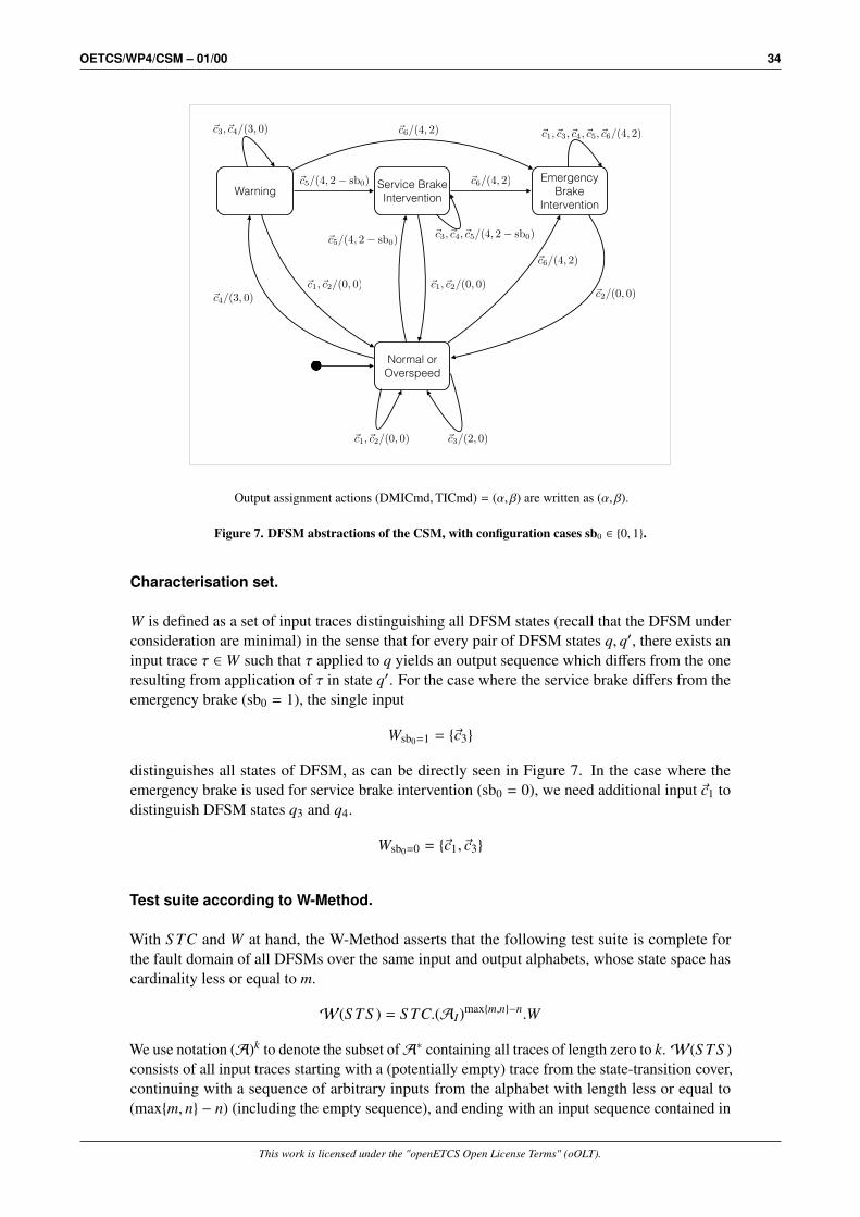
OETCS/WP4/CSM – 01/00 34
Normal or Overspeed
Warning Service Brake Intervention
Emergency Brake
Intervention
~c3/(2, 0)~c1,~c2/(0, 0)
~c4/(3, 0)~c1,~c2/(0, 0) ~c1,~c2/(0, 0)
~c2/(0, 0)
~c5/(4, 2 � sb0)
~c6/(4, 2)
~c6/(4, 2)
~c6/(4, 2)~c5/(4, 2 � sb0)
~c1,~c3,~c4,~c5,~c6/(4, 2)~c3,~c4/(3, 0)
~c3,~c4,~c5/(4, 2 � sb0)
Output assignment actions (DMICmd,TICmd) = (α, β) are written as (α, β).
Figure 7. DFSM abstractions of the CSM, with configuration cases sb0 ∈ {0, 1}.
Characterisation set.
W is defined as a set of input traces distinguishing all DFSM states (recall that the DFSM underconsideration are minimal) in the sense that for every pair of DFSM states q, q′, there exists aninput trace τ ∈ W such that τ applied to q yields an output sequence which differs from the oneresulting from application of τ in state q′. For the case where the service brake differs from theemergency brake (sb0 = 1), the single input
Wsb0=1 = {~c3}
distinguishes all states of DFSM, as can be directly seen in Figure 7. In the case where theemergency brake is used for service brake intervention (sb0 = 0), we need additional input ~c1 todistinguish DFSM states q3 and q4.
Wsb0=0 = {~c1, ~c3}
Test suite according to W-Method.
With S TC and W at hand, the W-Method asserts that the following test suite is complete forthe fault domain of all DFSMs over the same input and output alphabets, whose state space hascardinality less or equal to m.
W(S TS ) = S TC.(AI)max{m,n}−n.W
We use notation (A)k to denote the subset ofA∗ containing all traces of length zero to k.W(S TS )consists of all input traces starting with a (potentially empty) trace from the state-transition cover,continuing with a sequence of arbitrary inputs from the alphabet with length less or equal to(max{m, n} − n) (including the empty sequence), and ending with an input sequence contained in
This work is licensed under the "openETCS Open License Terms" (oOLT).

OETCS/WP4/CSM – 01/00 35
the transition cover. (A)0 just contains the empty trace, soW(S TS ) is reduced to S TC.W, ifthe fault domain of DFSM whose state space is less or equal to that of the reference DFSM isconsidered.
Assuming that the minimal DFSM associated with the SUT implements at most two additionalstates (m − n ≤ 2 implies m ≤ 6), the W-Method produces the following test suite for the theminimal DFSM:
S TC.(AI)2.Wsb0=1 = {~c3} ∪
{~ci.~c3 | i = 1, . . . , 6} ∪
{~ci.~c j.~c3 | i, j = 1, . . . , 6} ∪
{~ci.~c j.~ck.~c3 | i, j, k = 1, . . . , 6} ∪
{~c j.~ci.~c3 | i = 1, . . . , 6, j = 4, . . . , 6} ∪
{~c j.~ci.~ck.~c3 | i, k = 1, . . . , 6, j = 4, . . . , 6} ∪
{~c j.~ci.~ck.~ch.~c3 | h, i, k = 1, . . . , 6, j = 4, . . . , 6}
S TC.(AI)2.Wsb0=0 = {~cg | g = 1, 3} ∪
{~ci.~cg | i = 1, . . . , 6, g = 1, 3} ∪
{~ci.~c j.~cg | i, j = 1, . . . , 6, g = 1, 3} ∪
{~ci.~c j.~ch.~cg | h, i, j = 1, . . . , 6, g = 1, 3} ∪
{~c j.~ci.~cg | i = 1, . . . , 6, j = 4, . . . , 6, g = 1, 3} ∪
{~c j.~ci.~ck.~cg | i, k = 1, . . . , 6, j = 4, . . . , 6, g = 1, 3} ∪
{~c j.~ci.~ck.~ch.~cg | h, i, k = 1, . . . , 6, j = 4, . . . , 6, g = 1, 3}
Since ι-equivalence implies τ-equivalence when τ is a prefix of ι, the test suite produced by theW-Method can be reduced to the following:
TEST_SUITEsb0=1 = {~ci.~c j.~ck.~c3 | i, j, k = 1, . . . , 6} ∪
{~c j.~ci.~ck.~ch.~c3 | h, i, k = 1, . . . , 6, j = 4, . . . , 6}
TEST_SUITEsb0=0 = {~ci.~c j.~ch.~cg | h, i, j = 1, . . . , 6, g = 1, 3} ∪
{~c j.~ci.~ck.~ch.~cg | h, i, k = 1, . . . , 6, j = 4, . . . , 6, g = 1, 3}
8 Test Strength
8.1 Test Strength Assessment
The notion of test strength refers to the capability of test suites to uncover errors in an SUT. TheIECP testing strategy considered here is associated with a well-defined test strength, specified bymeans of the fault model: all deviations of an SUT from I/O-equivalence to the reference modelS will be detected, provided that the true behaviour of the SUT can be specified by means of anSTS which is contained in the fault domain. Based on the fault domain, the discussion of teststrength is “transformed” into the question whether the size of the fault domain for which the testsuite has been created is sufficient to contain all erroneous behaviours we can reasonably expect.
This work is licensed under the "openETCS Open License Terms" (oOLT).
OETCS/WP4/CSM – 01/00 36
In the next three sections examples will be presented where the erroneous SUT behaviour canalready by uncovered with IECP test suites based on the fault domain D(S,m = 6,I2 = I)specified in Section 6. The first example (Section 8.2) addresses a type of erroneous behaviourthat could not only be uncovered by the equivalence class testing strategy described in this report,but is also guaranteed to be detected by test suites achieving transition coverage of the SysMLstate machine model (see Section 10). The second example (Section 8.3) shows a type of failurethat is not guaranteed to be uncovered by test cases from a simple model coverage strategylike transition or MC/DC coverage, because it introduces an additional basic state in the SUT’sSysML state machine. Practical test execution documented in Section 10, however, shows thatthe failure is “accidentally” uncovered with the transition coverage strategy by the model-basedtesting tool used, due to suitable input values selected by the tool when trying to cover therequired transitions. The third example (Section 8.4) exhibits an even harder failure type, whichcannot be detected by any of the transition-based coverage strategies, as is documented by thetest results shown in Section 10.
In Section 9 we will discuss fault models associated with larger fault domains, based on truerefinements of I.
8.2 Example 1
Suppose that the implementation acts like the SysML state machine depicted in Fig. 8: frombasic state OVERSPEED there is a transition failure in the SysML state machine which links tobasic state EMER_BRAKE instead of NORMAL, when guard condition [Vest ≤ VMRSP] evaluatesto true. Note that the DFSM associated with S TS ′ now has one more state than the model’sDFSMs, because OVERSPEED and NORMAL are no longer equivalent.
Assuming the case sb0 = 1 and applying TEST_SUITEsb0=1 introduced in Section 7, this failurewill be uncovered, for example, by test case
ι = ~c1.~c3.~c1.~c3
= (Vest = 60,VMRSP = 90, allowRevokeEB = 0).(152, 150, 0).(60, 90, 0).(152, 150, 0)
On the model S TS , this input will trigger output sequence
(DMICmd = 0,TICmd = 0).(2, 0).(0, 0).(2, 0)
whereas output sequence
(DMICmd = 0,TICmd = 0).(2, 0).(4, 2).(4, 2)
will be triggered by ι, when applied to S TS ′ representing the SUT.
8.3 Example 2
Suppose that the implementation has an additional control state NORMAL_2, as depicted inFig. 9. When the SUT is in the control state OVERSPEED and inputs satisfy Vest ≤ VMRSP,the SUT’s state machine transits to the new basic state NORMAL_2. For this control state,there is only one outgoing transition whose guard condition is Vest > VMRSP + dVebi, and targetcontrol state is EMER_BRAKE. As a consequence, the SUT fails to issue warnings and totrigger service brake intervention, after having entered NORMAL_2; only the emergency brakeintervention condition is handled correctly. The SUT failure remains hidden until a transitionsequence from NORMAL to OVERSPEED and back to NORMAL should be performed. Notethat the introduction of this additional basic state in the SUT’s SysML state machine leads toa DFSM abstraction that has two more states than the DFSM abstraction of the original model,
This work is licensed under the "openETCS Open License Terms" (oOLT).

OETCS/WP4/CSM – 01/00 37
Figure 8. Faulty SUT – Example 1.
This work is licensed under the "openETCS Open License Terms" (oOLT).

OETCS/WP4/CSM – 01/00 38
because basic states NORMAL and OVERSPEED are no longer equivalent, and NORMAL_2 isnon-equivalent to any of the other states.
Assuming again the case sb0 = 1 and applying TEST_SUITEsb0=1 introduced in Section 7, thisfailure will be uncovered, for example, by test case
ι = ~c3.~c1.~c4.~c3
= (Vest = 152,VMRSP = 150, allowRevokeEB = 0).(60, 90, 0).(125, 120, 1).(152, 150, 0)
On the model S TS , this input will trigger output sequence
(DMICmd = 2,TICmd = 0).(0, 0).(3, 0).(3, 0)
whereas output sequence
(DMICmd = 2,TICmd = 0).(0, 0).(0, 0).(0, 0)
will be triggered by ι, when applied to S TS ′ representing the SUT.
Observe that this SUT failure would not be uncovered by every ordinary transition coveragetest strategy based on SysML state machine model. Transition coverage would be achieved, forexample, by the four test cases
TC_TEST_SUITE = {~c3.~c1, ~c3.~c4.~c1, ~c4.~c5.~c1, ~c5.~c6.~c2}
which fail to uncover the violation of I/O-equivalence.
8.4 Example 3
Suppose that the implementation has an additional control state NORMAL_2 as shown in themutant in Figure 10. When the SUT is in the control state Warning and inputs satisfy Vest ≤
VMRSP, the SUT’s state machine transits to the new basic state NORMAL_2. For this control state,there is only one outgoing transition in SysML whose guard condition is Vest > VMRSP +dVwarning,and target control state is Warning. Note that the introduction of this additional basic state inthe SUT’s SysML state machine leads to a DFSM abstraction that has two more states than theDFSM abstraction of the original model, because basic states NORMAL and OVERSPEED areno longer equivalent, and NORMAL_2 is non-equivalent to any of the other states.
Assuming again the case sb0 = 1 and applying TEST_SUITEsb0=1 introduced in Section 7, thisfailure will be uncovered, for example, by test case
ι = ~c4.~c1.~c3
= (Vest = 125,VMRSP = 120, allowRevokeEB = 1).(60, 90, 0).(152, 150, 0)
On the model S TS , this input will trigger output sequence
(DMICmd = 3,TICmd = 0).(0, 0).(2, 0)
whereas output sequence
(DMICmd = 3,TICmd = 0).(0, 0).(0, 0)
will be triggered by ι, when applied to S TS ′ representing the SUT.
Observe that this SUT failure would not be uncovered by every ordinary transition coveragetest strategy based on SysML state machine model. Transition coverage would be achieved,for example, by the test procedure TP-002 in Section 10 which fail to uncover the violation ofI/O-equivalence.
This work is licensed under the "openETCS Open License Terms" (oOLT).

OETCS/WP4/CSM – 01/00 39
Figure 9. Faulty SUT – Example 2.
This work is licensed under the "openETCS Open License Terms" (oOLT).
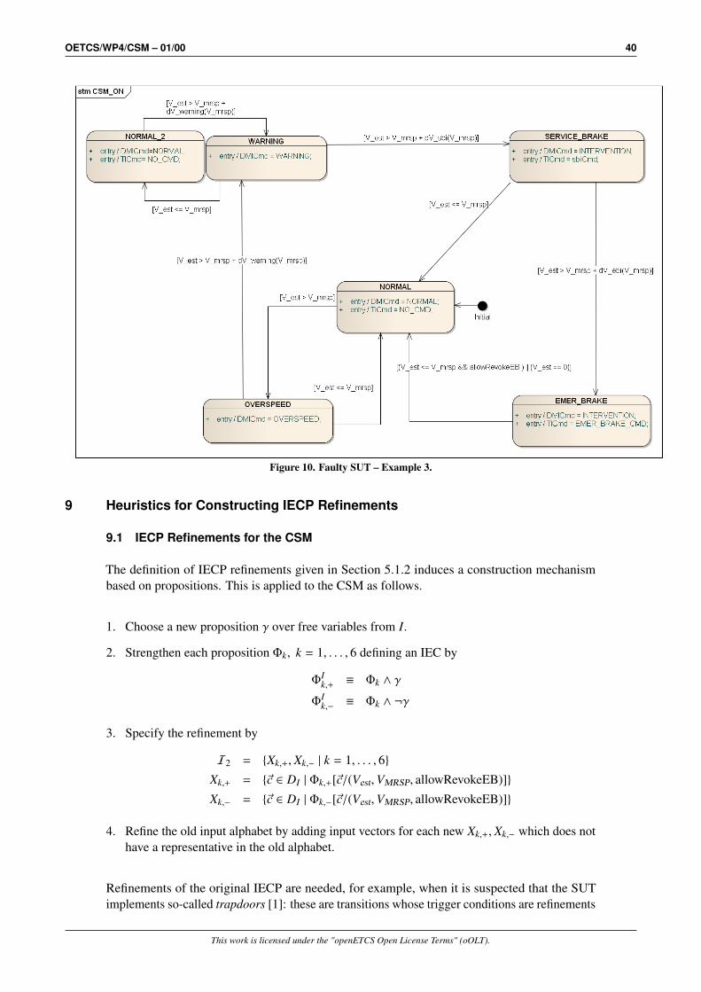
OETCS/WP4/CSM – 01/00 40
Figure 10. Faulty SUT – Example 3.
9 Heuristics for Constructing IECP Refinements
9.1 IECP Refinements for the CSM
The definition of IECP refinements given in Section 5.1.2 induces a construction mechanismbased on propositions. This is applied to the CSM as follows.
1. Choose a new proposition γ over free variables from I.
2. Strengthen each proposition Φk, k = 1, . . . , 6 defining an IEC by
ΦIk,+ ≡ Φk ∧ γ
ΦIk,− ≡ Φk ∧ ¬γ
3. Specify the refinement by
I2 = {Xk,+, Xk,− | k = 1, . . . , 6}
Xk,+ = {~c ∈ DI | Φk,+[~c/(Vest,VMRSP, allowRevokeEB)]}
Xk,− = {~c ∈ DI | Φk,−[~c/(Vest,VMRSP, allowRevokeEB)]}
4. Refine the old input alphabet by adding input vectors for each new Xk,+, Xk,− which does nothave a representative in the old alphabet.
Refinements of the original IECP are needed, for example, when it is suspected that the SUTimplements so-called trapdoors [1]: these are transitions whose trigger conditions are refinements
This work is licensed under the "openETCS Open License Terms" (oOLT).

OETCS/WP4/CSM – 01/00 41
ϕIq,i ∧ γ of trigger conditions ϕI
q,i in the original model. The SUT behaviour conforms to theassociated model transition for inputs satisfying ϕI
q,i ∧ ¬γ, but shows erroneous behaviour forinputs satisfying ϕI
q,i ∧ γ. Trapdoors may occur in transitions from quiescent to quiescent, and intransitions from quiescent to transient states. In the subsequent sections this and other motivationsfor introducing refinements are discussed.
9.2 Overview of the Refinement Concept
In this section we present and discuss a heuristic for constructing IECP refinements resulting inlarger fault domains that are well-justified from the perspective of standards related to safety-critical systems development in the avionic, automotive, and railway domains [26, 30, 14, 3].
Our heuristic involves the following refinement steps, and we suggest to apply these in the orderpresented here.
1. Requirements-based IECP refinement
2. Boundary value IECP refinement
3. IECP refinement by sub-paving
9.3 Requirements-based IECP Refinement
9.3.1 Requirements-related Case Distinctions
In Section 4.7.5 we introduced the transient state input conditions ϕIq,i. Intuitively speaking, each
of these conditions, when feasible and applied in quiescent state class q, triggers a well-definedbehaviour, namely the transformation of internal state and outputs performed by the transitionfrom transient state class Bi to its quiescent successor state class Ai. Since this transformationis constant (it only depends on Bi), it reflects one system requirement or a part of it. As aconsequence, any disjunction occurring in such a condition ϕI
q,i reflects a case distinction for thesame requirement.
Example Condition
ϕI0,1(V) ≡ VMRSP < Vest ∧ Vest ≤ VMRSP + dVwarning(VMRSP)
reflects the pre-condition for requirement REQ-3.13.10.3.3.t2 (see Table 2), concerning thetransition from NORMAL state to OVERSPEED state in the SysML state machine, with activationof the overspeed indication at the driver machine interface. ϕI
0,1(V) is applied in A0, and triggersa transition into B1 from where the overspeed indication is activated and the system stabilisesagain in A1. Expanding dVwarning(VMRSP), we get
ϕI0,1(V) ≡ VMRSP < Vest ∧
((VMRSP ≤ 110 ∧ Vest ≤ VMRSP + 4) ∨
(110 < VMRSP ≤ 140 ∧ Vest ≤3130
VMRSP +13
) ∨
(140 < VMRSP ∧ Vest ≤ VMRSP + 5))
The disjunction inside the second conjunct covers the three case distinctions for transiting intoOVERSPEED (see definition of dVwarning(VMRSP) in Equation (2)). �
This work is licensed under the "openETCS Open License Terms" (oOLT).
OETCS/WP4/CSM – 01/00 42
Similarly, the quiescent state conditions ϕIi (I) = ϕI
i,i(I) specify stability requirements regardinginput changes that will not lead to any new system reaction, so disjunctions in ϕI
i,i(I) representcase distinctions of these stability requirements.
Example Condition
ϕI4(V) ≡ ϕI
4,4(V) ≡ (0 < Vest ∧ allowRevokeEB = 0) ∨ (VMRSP < Vest ∧ allowRevokeEB = 1)
describes the stability condition when in SysML state machine state EMER_BRAKE. There aretwo cases to consider.
1. When the emergency brake command may only be revoked after the train has come to astandstill (case allowRevokeEB = 0), any input condition satisfying 0 < Vest is a stabilitycondition when in basic state EMER_BRAKE.
2. When the emergency brake command may already be revoked as soon as Vest ≤ VMRSP (caseallowRevokeEB = 1), any input condition satisfying VMRSP < Vest is a stability conditionwhen in basic state EMER_BRAKE.
�
Standards for safety-relevant systems always demand that requirements should be completelycovered by tests (see, e.g.,[30, 6.4.4]). Therefore it is advisable to refine the IECP in such a way,that the extended input alphabet resulting from this refinement covers all requirements-relatedcase distinctions.
9.3.2 Construction of the Requirements-based IECP Refinement
The mechanisable construction of the requirements-based IECP refinement is performed for theCSM as follows.
1. Transform each ϕIq,i and each ϕI
i,i into disjunctive normal form (DNF). This results in disjunctsϕI
q,i,h, such that
ϕIq,i ≡
∨j
ϕIq,i,h
Define index set Iq as the set of all pairs (i, h) where ϕIq,i,h is a disjunct in the DNF of ϕI
q,i.
2. Drop infeasible disjuncts. This can be performed by means of an SMT solver determining foreach disjunct whether it has at least one solution.
3. Refine the Φk, k = 1, . . . , 6 specifying the IECP of the CSM as described in Section 5.2.2 topropositions
Φk,( j0,h0),...,( j4,h4) ≡
4∧q=0
ϕIq, jq,hq
where ( jq, hq) ∈ Iq, q = 0, . . . , 4.
4. Create IECs in analogy to the rules given in Section 5.1.2, but this time using feasiblesolutions Φk,( j0,h0),...,( j4,h4):
Xk,( j0,h0),...,( j4,h4) = {~c ∈ DI | Φk,( j0,h0),...,( j4,h4)[~c/(Vest,VMRSP, allowRevokeEB)]}
This work is licensed under the "openETCS Open License Terms" (oOLT).

OETCS/WP4/CSM – 01/00 43
5. Determine the Xk,( j0,h0),...,( j4,h4) that are already represented by the existing members ~c of theold alphabet.
6. For each of the remaining Xk,( j0,h0),...,( j4,h4), select a new member for the new, extended inputalphabet by letting a constraint solver find a solution ~c for
Φk,( j0,h0),...,( j4,h4)[~c/(Vest,VMRSP, allowRevokeEB)]
Example For the CSM, the requirements-based IECP-refinement leads to the following disjunctsϕI
q,i, j.
ϕI0,0,0 ≡ ϕI
0(V) ≡ Vest ≤ VMRSP
ϕI1,1,0 ≡ VMRSP ≤ 110 ∧ VMRSP < Vest ≤ VMRSP + 4
ϕI1,1,1 ≡ 110 < VMRSP ≤ 140 ∧ VMRSP < Vest ≤
3130
VMRSP +13
ϕI1,1,2 ≡ 140 < VMRSP ∧ VMRSP < Vest ≤ VMRSP + 5
ϕI2,2,0 ≡ VMRSP ≤ 110 ∧ VMRSP < Vest ≤ VMRSP + 5.5
ϕI2,2,1 ≡ 110 < VMRSP ≤ 210 ∧ VMRSP < Vest ≤
209200
VMRSP +55
100ϕI
2,2,2 ≡ 210 < VMRSP ∧ VMRSP < Vest ≤ VMRSP + 10
ϕI3,3,0 ≡ VMRSP ≤ 110 ∧ VMRSP < Vest ≤ VMRSP + 7.5
ϕI3,3,1 ≡ 110 < VMRSP ≤ 210 ∧ VMRSP < Vest ≤
4340
VMRSP −34
ϕI3,3,2 ≡ 210 < VMRSP ∧ VMRSP < Vest ≤ VMRSP + 15
ϕI4,4,0 ≡ 0 < Vest ≤ VMRSP ∧ allowRevokeEB = 0
ϕI4,4,1 ≡ VMRSP < Vest
ϕI0,1,0 ≡ VMRSP ≤ 110 ∧ VMRSP < Vest ≤ VMRSP + 4
ϕI0,1,1 ≡ 110 < VMRSP ≤ 140 ∧ VMRSP < Vest ≤
3130
VMRSP +13
ϕI0,1,2 ≡ 140 < VMRSP ∧ VMRSP < Vest ≤ VMRSP + 5
ϕI0,2,0 ≡ VMRSP ≤ 110 ∧ VMRSP + 4 < Vest ≤ VMRSP + 5.5
ϕI0,2,1 ≡ 110 < VMRSP ≤ 140 ∧
3130
VMRSP +13< Vest ≤
209200
VMRSP +55100
ϕI0,2,2 ≡ 140 < VMRSP ≤ 210 ∧ VMRSP + 5 < Vest ≤
209200
VMRSP +55
100ϕI
0,2,3 ≡ 210 < VMRSP ∧ VMRSP + 5 < Vest ≤ VMRSP + 10
ϕI0,3,0 ≡ VMRSP ≤ 110 ∧ VMRSP + 5.5 < Vest ≤ VMRSP + 7.5
ϕI0,3,1 ≡ 110 < VMRSP ≤ 210 ∧
209200
VMRSP +55100
< Vest ≤4340
VMRSP −34
ϕI0,3,2 ≡ 210 < VMRSP ∧ VMRSP + 10 < Vest ≤ VMRSP + 15
ϕI0,4,0 ≡ VMRSP ≤ 110 ∧ VMRSP + 7.5 < Vest
ϕI0,4,1 ≡ 110 < VMRSP ≤ 210 ∧
4340
VMRSP −34< Vest
ϕI0,4,2 ≡ 210 < VMRSP ∧ VMRSP + 15 < Vest
This work is licensed under the "openETCS Open License Terms" (oOLT).

OETCS/WP4/CSM – 01/00 44
ϕI1,2,i ≡ ϕI
0,2,i, i = 0, 1, 2, 3
ϕI1,3,i ≡ ϕI
0,3,i, i = 0, 1, 2
ϕI1,4,i ≡ ϕI
0,4,i, i = 0, 1, 2
ϕI2,3,i ≡ ϕI
0,3,i i = 0, 1, 2
ϕI2,4,i ≡ ϕI
0,4,i i = 0, 1, 2
ϕI3,4,i ≡ ϕI
0,4,i i = 0, 1, 2
ϕI1,0,0 ≡ ϕ1,0 ≡ Vest ≤ VMRSP
ϕI2,0,0 ≡ ϕI
1,0,0
ϕI3,0,0 ≡ ϕI
1,0,0
ϕI4,0,0 ≡ Vest = 0
ϕI4,0,1 ≡ 0 < Vest ≤ VMRSP ∧ allowRevokeEB = 1
This leads to the following refined predicates Φi j .
Φ10 ≡ ϕI0,0,0 ∧ ϕ
I1,0,0 ∧ ϕ
I2,0,0 ∧ ϕ
I3,0,0 ∧ ϕ
I4,4,0
≡ ϕI0,0,0 ∧ ϕ
I4,4,0
≡ 0 < Vest ≤ VMRSP ∧ allowRevokeEB = 0
Φ20 ≡ ϕI0,0,0 ∧ ϕ
I1,0,0 ∧ ϕ
I2,0,0 ∧ ϕ
I3,0,0 ∧ ϕ
I4,0,0
≡ ϕI4,0,0
≡ Vest = 0
Φ21 ≡ ϕI0,0,0 ∧ ϕ
I1,0,0 ∧ ϕ
I2,0,0 ∧ ϕ
I3,0,0 ∧ ϕ
I4,0,1
≡ ϕI4,0,1
≡ 0 < Vest ≤ VMRSP ∧ allowRevokeEB = 1
Φ30 ≡ ϕI0,1,0 ∧ ϕ
I1,1,0 ∧ ϕ
I2,2,0 ∧ ϕ
I3,3,0 ∧ ϕ
I4,4,1
≡ VMRSP ≤ 110 ∧ VMRSP < Vest ≤ VMRSP + 4
Φ31 ≡ ϕI0,1,1 ∧ ϕ
I1,1,1 ∧ ϕ
I2,2,1 ∧ ϕ
I3,3,1 ∧ ϕ
I4,4,1
≡ 110 < VMRSP ≤ 140 ∧ VMRSP < Vest ≤3130
VMRSP +13
Φ32 ≡ ϕI0,1,2 ∧ ϕ
I1,1,2 ∧ ϕ
I2,2,1 ∧ ϕ
I3,3,1 ∧ ϕ
I4,4,1
≡ 140 < VMRSP ≤ 210 ∧ VMRSP < Vest ≤ VMRSP + 5
This work is licensed under the "openETCS Open License Terms" (oOLT).

OETCS/WP4/CSM – 01/00 45
Φ33 ≡ ϕI0,1,2 ∧ ϕ
I1,1,2 ∧ ϕ
I2,2,2 ∧ ϕ
I3,3,2 ∧ ϕ
I4,4,1
≡ 210 < VMRSP < Vest ≤ VMRSP + 5
Φ40 ≡ ϕI0,2,0 ∧ ϕ
I1,2,0 ∧ ϕ
I2,2,0 ∧ ϕ
I3,3,0 ∧ ϕ
I4,4,1
≡ VMRSP ≤ 110 ∧ VMRSP + 4 < Vest ≤ VMRSP + 5.5
Φ41 ≡ ϕI0,2,1 ∧ ϕ
I1,2,1 ∧ ϕ
I2,2,1 ∧ ϕ
I3,3,1 ∧ ϕ
I4,4,1
≡ 110 < VMRSP ≤ 140 ∧3130
VMRSP +13< Vest ≤
209200
VMRSP +55100
Φ42 ≡ ϕI0,2,2 ∧ ϕ
I1,2,2 ∧ ϕ
I2,2,1 ∧ ϕ
I3,3,1 ∧ ϕ
I4,4,1
≡ 140 < VMRSP ≤ 210 ∧ VMRSP + 5 < Vest ≤209200
VMRSP +55100
Φ43 ≡ ϕI0,2,3 ∧ ϕ
I1,2,3 ∧ ϕ
I2,2,2 ∧ ϕ
I3,3,2 ∧ ϕ
I4,4,1
≡ 210 < VMRSP ∧ VMRSP + 5 < Vest ≤ VMRSP + 10
Φ50 ≡ ϕI0,3,0 ∧ ϕ
I1,3,0 ∧ ϕ
I2,3,0 ∧ ϕ
I3,3,0 ∧ ϕ
I4,4,1
≡ VMRSP ≤ 110 ∧ VMRSP + 5.5 < Vest ≤ VMRSP + 7.5
Φ51 ≡ ϕI0,3,1 ∧ ϕ
I1,3,1 ∧ ϕ
I2,3,1 ∧ ϕ
I3,3,1 ∧ ϕ
I4,4,1
≡ 110 < VMRSP ≤ 210 ∧209200
VMRSP +55
100< Vest ≤
4340
VMRSP −34
Φ52 ≡ ϕI0,3,2 ∧ ϕ
I1,3,2 ∧ ϕ
I2,3,2 ∧ ϕ
I3,3,2 ∧ ϕ
I4,4,1
≡ 210 < VMRSP ∧ VMRSP + 10 < Vest ≤ VMRSP + 15
Φ60 ≡ ϕI0,4,0 ∧ ϕ
I1,4,0 ∧ ϕ
I2,4,0 ∧ ϕ
I3,4,0 ∧ ϕ
I4,4,1
≡ VMRSP ≤ 110 ∧ VMRSP + 7.5 < Vest
Φ61 ≡ ϕI0,4,1 ∧ ϕ
I1,4,1 ∧ ϕ
I2,4,1 ∧ ϕ
I3,4,1 ∧ ϕ
I4,4,1
≡ 110 < VMRSP ≤ 210 ∧4340
VMRSP −34< Vest
Φ62 ≡ ϕI0,4,2 ∧ ϕ
I1,4,2 ∧ ϕ
I2,4,2 ∧ ϕ
I3,4,2 ∧ ϕ
I4,4,1
≡ 210 < VMRSP ∧ VMRSP + 15 < Vest
From the refined predicates additional members of the input alphabet are selected. This results ina new alphabet as the one shown in Table 11.
The resulting test suite comprises the test cases of the old suite plus additional cases, the newtest suite can be expressed as an extension of the old one. Since (A ∪ B)3 = A3 ∪ A2.B ∪A.B.(A ∪ B) ∪ B.(A ∪ B)2, for any subsets A, B of the input alphabet, the old input alphabet withset A = {c1, . . . , c6}, and the new alphabet values contained in B = {c7, . . . , c17} result in thefollowing test suite.
TEST_SUITEsb0=1′ = {~ci.~c j.~ck.~c3 | i, j, k = 1, . . . , 17} ∪
{~c j.~ci.~ck.~ch.~c3 | h, i, k = 1, . . . , 17, j = 4, 5, 6} ∪
= {~ci.~c j.~ck.~c3 | i, j, k = 1, . . . , 6} ∪
{~c j.~ci.~ck.~ch.~c3 | h, i, k = 1, . . . , 6, j = 4, 5, 6} ∪
{~ci.~c j.~ck.~c3 | i, j = 1, . . . , 6, k = 7, . . . , 17} ∪
{~ci.~ck.~c j.~c3 | i = 1, . . . , 6, j = 1, . . . , 17, k = 7, . . . , 17} ∪
{~ck.~ci.~c j.~c3 | i, j = 1, . . . , 17, k = 7, . . . , 17} ∪
{~c j.~ci.~ch.~ck.~c3 | i, h = 1, . . . , 6, k = 7, . . . , 17, j = 4, 5, 6} ∪
{~c j.~ci.~ck.~ch.~c3 | i = 1, . . . , 6, h = 1, . . . , 17, k = 7, . . . , 17, j = 4, 5, 6} ∪
{~c j.~ck.~ci.~ch.~c3 | i, h = 1, . . . , 17, k = 7, . . . , 17, j = 4, 5, 6}
�
This work is licensed under the "openETCS Open License Terms" (oOLT).
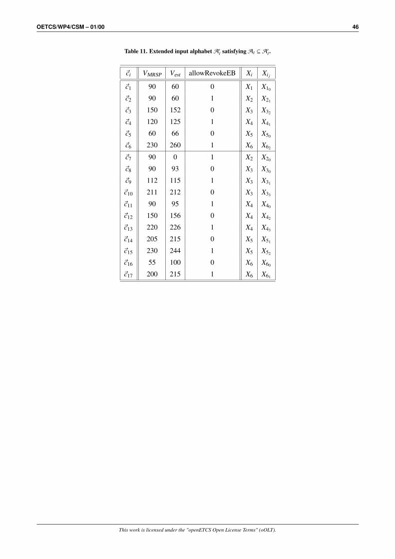
OETCS/WP4/CSM – 01/00 46
Table 11. Extended input alphabetA′I satisfyingAI ⊆ A′I .
~ci VMRSP Vest allowRevokeEB Xi Xi j
~c1 90 60 0 X1 X10
~c2 90 60 1 X2 X21
~c3 150 152 0 X3 X32
~c4 120 125 1 X4 X41
~c5 60 66 0 X5 X50
~c6 230 260 1 X6 X62
~c7 90 0 1 X2 X20
~c8 90 93 0 X3 X30
~c9 112 115 1 X3 X31
~c10 211 212 0 X3 X33
~c11 90 95 1 X4 X40
~c12 150 156 0 X4 X42
~c13 220 226 1 X4 X43
~c14 205 215 0 X5 X51
~c15 230 244 1 X5 X52
~c16 55 100 0 X6 X60
~c17 200 215 1 X6 X61
This work is licensed under the "openETCS Open License Terms" (oOLT).

OETCS/WP4/CSM – 01/00 47
9.3.3 Discussion
The requirements-based IECP refinement ensures that all case distinctions of requirements aretested. As a consequence, all SUT failures will be detected, where in a certain SUT state allinputs that should trigger the reaction for a given requirements sub-case are handled incorrectly.Compared to the original IECP, this is a considerable improvement, because the original IECP isonly guaranteed to detect failures if all sub-cases of a requirement are incorrectly handled by theSUT in a certain state.
Just as for the original IECP, however, the requirements-based IECP refinement relies on theSUT implementing all control decisions, that is, all guard conditions specified in the originalSysML state machine, correctly. Failures are only allowed in the actions setting outputs andinternal states. This is of considerable value if SUT code is generated semi-automatically. Aqualified code-frame generator, for example, might derive a control procedure from the statemachine model, so that all control states, guard conditions, and state machine transitions aregenerated with high reliability by the tool. However, the driver software implementing access tothe hardware output interfaces – in our example the DMI and the train interface acting on thebrakes – may have been implemented in a manual way, so that some actions will show erroneousbehaviour in certain states of the SUT.
For other development scenarios, in particular, when the SUT code has been developed from therequirements in manual way, the test strength of the requirements-based IECP refinement is stillinsufficient, because SUT failures in the handling of guard conditions are just as likely as failuresin the action implementations. These failure scenarios will be considered in the next refinements.
9.4 Boundary Value IECP Refinement
Let I2 = {X10 , X20 , X21 , . . . , X62} be the input equivalence class partitioning containing the 17input equivalence classes constructed above by Φi j . Extend the old input alphabet to a newinput alphabet which includes input vectors of the boundary of each Xi j . Then the new inputalphabet (see Table 12) contains 31 inputs more then the old one, and the new test suite contains4 · 483 = 442368 test cases, 4 · 483 − 4 · 173 = 442368 − 19652 = 422716 test cases more.
Since the CSM code does not depend on dealt-time conditions, this is still an acceptable numberof software tests. For hardware-in-the-loop tests, when timing constraints of the target hardwareand the operational environment have to be considered, however, it would be too time-consumingto execute them all. A well-justified reduction heuristic in this case is to drop the tests of certainboundary values for states where these boundaries are of no relevance.
This work is licensed under the "openETCS Open License Terms" (oOLT).
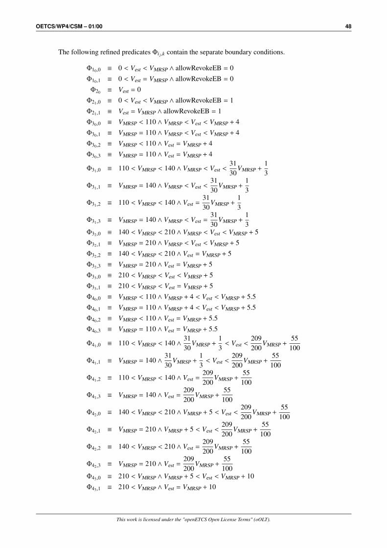
OETCS/WP4/CSM – 01/00 48
The following refined predicates Φi j,k contain the separate boundary conditions.
Φ10,0 ≡ 0 < Vest < VMRSP ∧ allowRevokeEB = 0
Φ10,1 ≡ 0 < Vest = VMRSP ∧ allowRevokeEB = 0
Φ20 ≡ Vest = 0
Φ21,0 ≡ 0 < Vest < VMRSP ∧ allowRevokeEB = 1
Φ21,1 ≡ Vest = VMRSP ∧ allowRevokeEB = 1
Φ30,0 ≡ VMRSP < 110 ∧ VMRSP < Vest < VMRSP + 4
Φ30,1 ≡ VMRSP = 110 ∧ VMRSP < Vest < VMRSP + 4
Φ30,2 ≡ VMRSP < 110 ∧ Vest = VMRSP + 4
Φ30,3 ≡ VMRSP = 110 ∧ Vest = VMRSP + 4
Φ31,0 ≡ 110 < VMRSP < 140 ∧ VMRSP < Vest <3130
VMRSP +13
Φ31,1 ≡ VMRSP = 140 ∧ VMRSP < Vest <3130
VMRSP +13
Φ31,2 ≡ 110 < VMRSP < 140 ∧ Vest =3130
VMRSP +13
Φ31,3 ≡ VMRSP = 140 ∧ VMRSP < Vest =3130
VMRSP +13
Φ32,0 ≡ 140 < VMRSP < 210 ∧ VMRSP < Vest < VMRSP + 5
Φ32,1 ≡ VMRSP = 210 ∧ VMRSP < Vest < VMRSP + 5
Φ32,2 ≡ 140 < VMRSP < 210 ∧ Vest = VMRSP + 5
Φ32,3 ≡ VMRSP = 210 ∧ Vest = VMRSP + 5
Φ33,0 ≡ 210 < VMRSP < Vest < VMRSP + 5
Φ33,1 ≡ 210 < VMRSP < Vest = VMRSP + 5
Φ40,0 ≡ VMRSP < 110 ∧ VMRSP + 4 < Vest < VMRSP + 5.5
Φ40,1 ≡ VMRSP = 110 ∧ VMRSP + 4 < Vest < VMRSP + 5.5
Φ40,2 ≡ VMRSP < 110 ∧ Vest = VMRSP + 5.5
Φ40,3 ≡ VMRSP = 110 ∧ Vest = VMRSP + 5.5
Φ41,0 ≡ 110 < VMRSP < 140 ∧3130
VMRSP +13< Vest <
209200
VMRSP +55100
Φ41,1 ≡ VMRSP = 140 ∧3130
VMRSP +13< Vest <
209200
VMRSP +55100
Φ41,2 ≡ 110 < VMRSP < 140 ∧ Vest =209200
VMRSP +55100
Φ41,3 ≡ VMRSP = 140 ∧ Vest =209200
VMRSP +55100
Φ42,0 ≡ 140 < VMRSP < 210 ∧ VMRSP + 5 < Vest <209200
VMRSP +55100
Φ42,1 ≡ VMRSP = 210 ∧ VMRSP + 5 < Vest <209200
VMRSP +55
100
Φ42,2 ≡ 140 < VMRSP < 210 ∧ Vest =209200
VMRSP +55100
Φ42,3 ≡ VMRSP = 210 ∧ Vest =209200
VMRSP +55100
Φ43,0 ≡ 210 < VMRSP ∧ VMRSP + 5 < Vest < VMRSP + 10
Φ43,1 ≡ 210 < VMRSP ∧ Vest = VMRSP + 10
This work is licensed under the "openETCS Open License Terms" (oOLT).
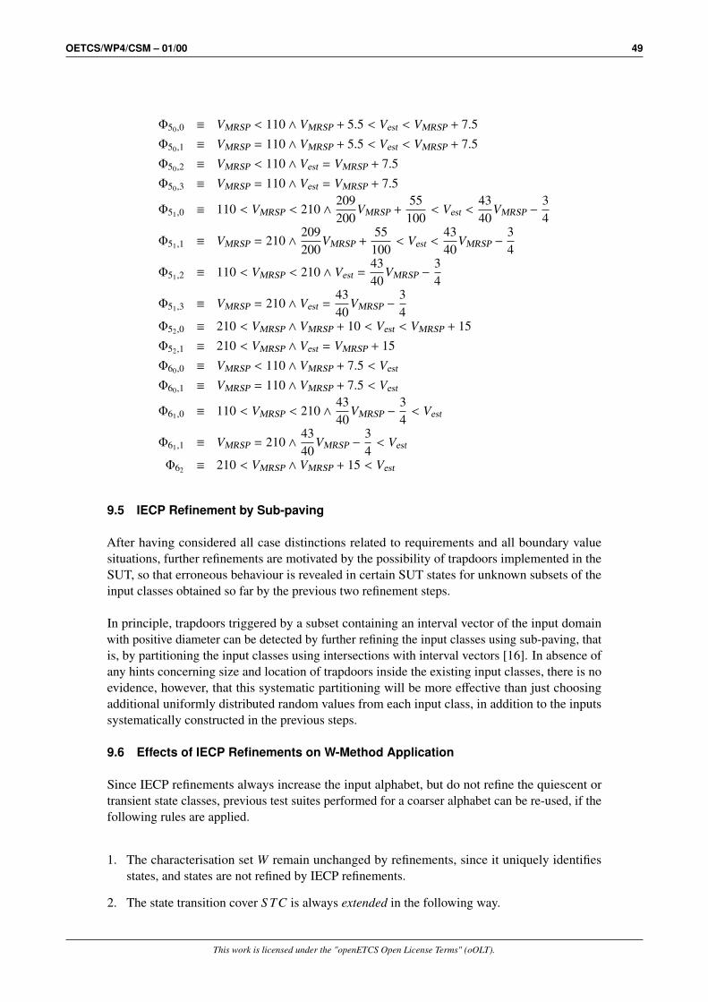
OETCS/WP4/CSM – 01/00 49
Φ50,0 ≡ VMRSP < 110 ∧ VMRSP + 5.5 < Vest < VMRSP + 7.5
Φ50,1 ≡ VMRSP = 110 ∧ VMRSP + 5.5 < Vest < VMRSP + 7.5
Φ50,2 ≡ VMRSP < 110 ∧ Vest = VMRSP + 7.5
Φ50,3 ≡ VMRSP = 110 ∧ Vest = VMRSP + 7.5
Φ51,0 ≡ 110 < VMRSP < 210 ∧209200
VMRSP +55100
< Vest <4340
VMRSP −34
Φ51,1 ≡ VMRSP = 210 ∧209200
VMRSP +55100
< Vest <4340
VMRSP −34
Φ51,2 ≡ 110 < VMRSP < 210 ∧ Vest =4340
VMRSP −34
Φ51,3 ≡ VMRSP = 210 ∧ Vest =4340
VMRSP −34
Φ52,0 ≡ 210 < VMRSP ∧ VMRSP + 10 < Vest < VMRSP + 15
Φ52,1 ≡ 210 < VMRSP ∧ Vest = VMRSP + 15
Φ60,0 ≡ VMRSP < 110 ∧ VMRSP + 7.5 < Vest
Φ60,1 ≡ VMRSP = 110 ∧ VMRSP + 7.5 < Vest
Φ61,0 ≡ 110 < VMRSP < 210 ∧4340
VMRSP −34< Vest
Φ61,1 ≡ VMRSP = 210 ∧4340
VMRSP −34< Vest
Φ62 ≡ 210 < VMRSP ∧ VMRSP + 15 < Vest
9.5 IECP Refinement by Sub-paving
After having considered all case distinctions related to requirements and all boundary valuesituations, further refinements are motivated by the possibility of trapdoors implemented in theSUT, so that erroneous behaviour is revealed in certain SUT states for unknown subsets of theinput classes obtained so far by the previous two refinement steps.
In principle, trapdoors triggered by a subset containing an interval vector of the input domainwith positive diameter can be detected by further refining the input classes using sub-paving, thatis, by partitioning the input classes using intersections with interval vectors [16]. In absence ofany hints concerning size and location of trapdoors inside the existing input classes, there is noevidence, however, that this systematic partitioning will be more effective than just choosingadditional uniformly distributed random values from each input class, in addition to the inputssystematically constructed in the previous steps.
9.6 Effects of IECP Refinements on W-Method Application
Since IECP refinements always increase the input alphabet, but do not refine the quiescent ortransient state classes, previous test suites performed for a coarser alphabet can be re-used, if thefollowing rules are applied.
1. The characterisation set W remain unchanged by refinements, since it uniquely identifiesstates, and states are not refined by IECP refinements.
2. The state transition cover S TC is always extended in the following way.
This work is licensed under the "openETCS Open License Terms" (oOLT).
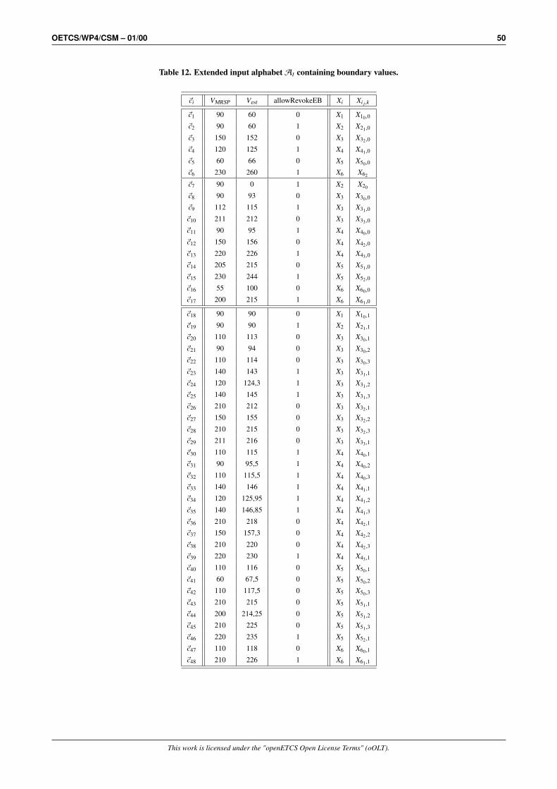
OETCS/WP4/CSM – 01/00 50
Table 12. Extended input alphabetAI containing boundary values.
~ci VMRSP Vest allowRevokeEB Xi Xi j ,k
~c1 90 60 0 X1 X10 ,0
~c2 90 60 1 X2 X21 ,0
~c3 150 152 0 X3 X32 ,0
~c4 120 125 1 X4 X41 ,0
~c5 60 66 0 X5 X50 ,0
~c6 230 260 1 X6 X62
~c7 90 0 1 X2 X20
~c8 90 93 0 X3 X30 ,0
~c9 112 115 1 X3 X31 ,0
~c10 211 212 0 X3 X33 ,0
~c11 90 95 1 X4 X40 ,0
~c12 150 156 0 X4 X42 ,0
~c13 220 226 1 X4 X43 ,0
~c14 205 215 0 X5 X51 ,0
~c15 230 244 1 X5 X52 ,0
~c16 55 100 0 X6 X60 ,0
~c17 200 215 1 X6 X61 ,0
~c18 90 90 0 X1 X10 ,1
~c19 90 90 1 X2 X21 ,1
~c20 110 113 0 X3 X30 ,1
~c21 90 94 0 X3 X30 ,2
~c22 110 114 0 X3 X30 ,3
~c23 140 143 1 X3 X31 ,1
~c24 120 124,3 1 X3 X31 ,2
~c25 140 145 1 X3 X31 ,3
~c26 210 212 0 X3 X32 ,1
~c27 150 155 0 X3 X32 ,2
~c28 210 215 0 X3 X32 ,3
~c29 211 216 0 X3 X33 ,1
~c30 110 115 1 X4 X40 ,1
~c31 90 95,5 1 X4 X40 ,2
~c32 110 115,5 1 X4 X40 ,3
~c33 140 146 1 X4 X41 ,1
~c34 120 125,95 1 X4 X41 ,2
~c35 140 146,85 1 X4 X41 ,3
~c36 210 218 0 X4 X42 ,1
~c37 150 157,3 0 X4 X42 ,2
~c38 210 220 0 X4 X42 ,3
~c39 220 230 1 X4 X43 ,1
~c40 110 116 0 X5 X50 ,1
~c41 60 67,5 0 X5 X50 ,2
~c42 110 117,5 0 X5 X50 ,3
~c43 210 215 0 X5 X51 ,1
~c44 200 214,25 0 X5 X51 ,2
~c45 210 225 0 X5 X51 ,3
~c46 220 235 1 X5 X52 ,1
~c47 110 118 0 X6 X60 ,1
~c48 210 226 1 X6 X61 ,1
This work is licensed under the "openETCS Open License Terms" (oOLT).
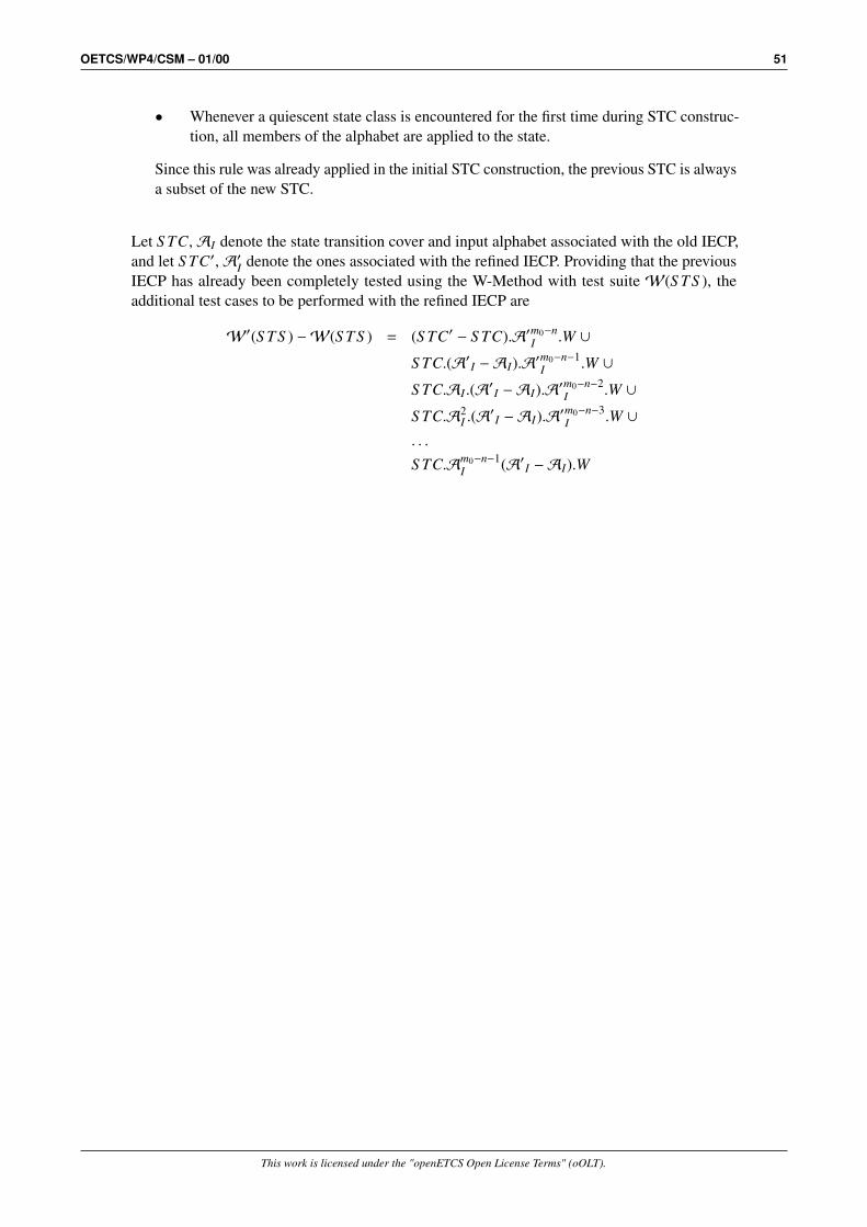
OETCS/WP4/CSM – 01/00 51
• Whenever a quiescent state class is encountered for the first time during STC construc-tion, all members of the alphabet are applied to the state.
Since this rule was already applied in the initial STC construction, the previous STC is alwaysa subset of the new STC.
Let S TC,AI denote the state transition cover and input alphabet associated with the old IECP,and let S TC′,A′I denote the ones associated with the refined IECP. Providing that the previousIECP has already been completely tested using the W-Method with test suite W(S TS ), theadditional test cases to be performed with the refined IECP are
W′(S TS ) −W(S TS ) = (S TC′ − S TC).A′m0−nI .W ∪
S TC.(A′I −AI).A′m0−n−1I .W ∪
S TC.AI .(A′I −AI).A′m0−n−2I .W ∪
S TC.A2I .(A
′I −AI).A′
m0−n−3I .W ∪
. . .
S TC.Am0−n−1I (A′I −AI).W
This work is licensed under the "openETCS Open License Terms" (oOLT).

OETCS/WP4/CSM – 01/00 52
10 Test Procedures
10.1 Test Automation Tool
The tests for the CSM provided under www.mbt-benchmarks.org have been performed withthe model-based testing component RTT-MBT of the test automation tool RT-Tester [23]. RT-Tester supports all test levels from unit testing to system integration testing and provides differentfunctions for manual test procedure development, automated test case, test data and test proceduregeneration, as well as management functions for large test campaigns. The typical applicationscope covers (potentially safety-critical) embedded real-time systems involving concurrency, timeconstraints, discrete control decisions as well as integer and floating point data and calculations.While the tool has been used in industry for about 15 years and has been qualified for avionic,automotive and railway control systems under test according to the standards [26, 15, 3], its MBTfunctionality is based on more recent extensions that have been validated during the last years invarious projects from the transportation domains and are now made available to the public.
10.2 Test Categories
The tests presented for the CSM under www.mbt-benchmarks.org can be structured according tothe following coverage strategies.
1. Test procedures aiming at basic state coverage
2. Test procedures aiming at transition coverage
3. Test procedures aiming at MC/DC coverage
4. Test procedures based on user defined test cases, aiming at requirements coverage
5. Test procedures based on input equivalence class partitioning principle described in thistechnical report. These are described in Section 10.4.
10.3 Tests of Categories 1 — 4
Table 13 summarises the coverage achieved by the generated tests of categories 1 — 4. Each testprocedure is duplicated to take into account the different values of the flag SBAvailable, exceptfor the test procedure TP-005 that checks the behaviour only when service brakes are available.TP-001-BCS is the test procedure realising the basic state coverage, TP-002-Transitions thetransition coverage and TP-003-MC/DC the MC/DC coverage. Requirement-based testing isperformed by the Test procedures TP-004 to TP-008. Table 14 defines the requirements associatedwith each test procedure. TP-004 focuses on the DMI interface. TP-005 provides a test to checkthe behaviour when the service brake is not available. TP-006 validates the special transitionwhen entering the ceiling speed monitoring with the indication status set to one. TP-007 andTP-008 are the test procedure for testing the revocation and the triggering of DMICmd andTICmd.
TP-002-OnlyCSM_ON, TP-002-OnlyCSM_ON-SNOSB
These two test procedures generated by the tool have allowRevokeEB equals 0 and are of theform specified in Table 15 and Table 16. The two test procedures are able to kill the mutant inExample 1 thanks to the sequence NORMAL→ OVERSPEED→ NORMAL. The second mutant isnot killed by the first test procedure but the sequence NORMAL→ OVERSPEED→WARNING in
This work is licensed under the "openETCS Open License Terms" (oOLT).

OETCS/WP4/CSM – 01/00 53
Table 13. Test procedures
TP Name MCDC UD HITR TR BCS REQ
TP-001-BCS 42% 15% 0% 45% 100% 12%
TP-001-BCS-NOSB 42% 15% 0% 45% 100% 12%
TP-002-OnlyCSM_ON 57% 23% 0% 81% 100% 40%
TP-002-OnlyCSM_ON-NOSB 57% 23% 0% 81% 100% 36%
TP-002-Transition 64% 38% 100% 90% 100% 56%
TP-002-Transition-NOSB 78% 23% 100% 100% 100% 52%
TP-003-MCDC 85% 15% 0% 54% 100% 20%
TP-003-MCDC-NOSB 85% 30% 0% 54% 100% 20%
TP-004-3.13.10-DMIOutputs 85% 46% 100% 90% 100% 80%
TP-004-3.13.10-DMIOutputs-NOSB 85% 61% 100% 90% 100% 80%
TP-005-3.13.10-EBvsSB 64% 30% 20% 90% 100% 48%
TP-006-3.13.10-IndicationStatus 57% 38% 60% 63% 100% 24%
TP-006-3.13.10-IndicationStatus-NOSB 57% 46% 60% 63% 100% 28%
TP-007-3.13.10-RevokeCmd 57% 15% 0% 81% 100% 36%
TP-007-3.13.10-RevokeCmd-NOSB 64% 30% 0% 81% 100% 36%
TP-008-3.13.10-Trigger 85% 38% 100% 90% 100% 76%
TP-008-3.13.10-Trigger-NOSB 85% 69% 100% 90% 100% 84%
This work is licensed under the "openETCS Open License Terms" (oOLT).
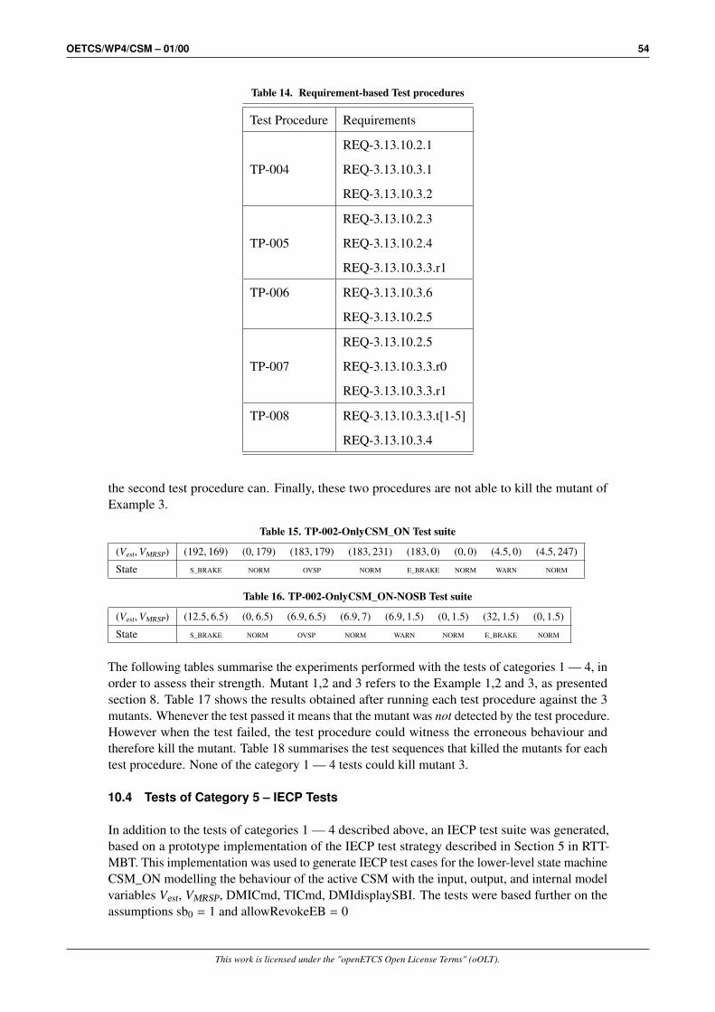
OETCS/WP4/CSM – 01/00 54
Table 14. Requirement-based Test procedures
Test Procedure Requirements
REQ-3.13.10.2.1
TP-004 REQ-3.13.10.3.1
REQ-3.13.10.3.2
REQ-3.13.10.2.3
TP-005 REQ-3.13.10.2.4
REQ-3.13.10.3.3.r1
TP-006 REQ-3.13.10.3.6
REQ-3.13.10.2.5
REQ-3.13.10.2.5
TP-007 REQ-3.13.10.3.3.r0
REQ-3.13.10.3.3.r1
TP-008 REQ-3.13.10.3.3.t[1-5]
REQ-3.13.10.3.4
the second test procedure can. Finally, these two procedures are not able to kill the mutant ofExample 3.
Table 15. TP-002-OnlyCSM_ON Test suite
(Vest,VMRSP) (192, 169) (0, 179) (183, 179) (183, 231) (183, 0) (0, 0) (4.5, 0) (4.5, 247)
State S_BRAKE NORM OVSP NORM E_BRAKE NORM WARN NORM
Table 16. TP-002-OnlyCSM_ON-NOSB Test suite
(Vest,VMRSP) (12.5, 6.5) (0, 6.5) (6.9, 6.5) (6.9, 7) (6.9, 1.5) (0, 1.5) (32, 1.5) (0, 1.5)
State S_BRAKE NORM OVSP NORM WARN NORM E_BRAKE NORM
The following tables summarise the experiments performed with the tests of categories 1 — 4, inorder to assess their strength. Mutant 1,2 and 3 refers to the Example 1,2 and 3, as presentedsection 8. Table 17 shows the results obtained after running each test procedure against the 3mutants. Whenever the test passed it means that the mutant was not detected by the test procedure.However when the test failed, the test procedure could witness the erroneous behaviour andtherefore kill the mutant. Table 18 summarises the test sequences that killed the mutants for eachtest procedure. None of the category 1 — 4 tests could kill mutant 3.
10.4 Tests of Category 5 – IECP Tests
In addition to the tests of categories 1 — 4 described above, an IECP test suite was generated,based on a prototype implementation of the IECP test strategy described in Section 5 in RTT-MBT. This implementation was used to generate IECP test cases for the lower-level state machineCSM_ON modelling the behaviour of the active CSM with the input, output, and internal modelvariables Vest, VMRSP, DMICmd, TICmd, DMIdisplaySBI. The tests were based further on theassumptions sb0 = 1 and allowRevokeEB = 0
This work is licensed under the "openETCS Open License Terms" (oOLT).

OETCS/WP4/CSM – 01/00 55
Table 17. Mutants experiments results
Test-Procedure Mutant 1 Mutant 2 Mutant 3
TP-001-BCS PASS PASS PASS
TP-001-BCS-NOSB PASS PASS PASS
TP-002-OnlyCSM_ON FAIL PASS PASS
TP-002-OnlyCSM_ON-NOSB FAIL FAIL PASS
TP-002-Transition FAIL FAIL PASS
TP-002-Transition-NOSB FAIL FAIL PASS
TP-003-MCDC PASS PASS PASS
TP-003-MCDC-NOSB PASS PASS PASS
TP-004-3.13.10-DMIOutput FAIL PASS PASS
TP-004-3.13.10-DMIOutput-NOSB FAIL PASS PASS
TP-005-3.13.10-EBvsSB FAIL PASS PASS
TP-006-3.13.10-IndicationStatus FAIL PASS PASS
TP-006-3.13.10-IndicationStatus-NOSB FAIL PASS PASS
TP-007-3.13.10-RevokeCmd FAIL FAIL PASS
TP-007-3.13.10-RevokeCmd-NOSB FAIL FAIL PASS
TP-008-3.13.10-Trigger FAIL FAIL PASS
TP-008-3.13.10-Trigger-NOSB FAIL FAIL PASS
Table 18. Test sequences that kills the mutant
Mutant Test Procedure sequences
Mutant 1
TP-002 NORM→ OVSP→NORM
TP-004 NORM→ OVSP→NORM
TP-005 NORM→ OVSP→NORM
TP-006 NORM→ OVSP→NORM
TP-007 NORM→ OVSP→NORM
TP-008 NORM→ OVSP→NORM
Mutant 2
TP-002 OVSP→ NORM→OVSP
TP-005 OVSP→ NORM→WARN
TP-007 OVSP→ NORM→WARN
TP-008 OVSP→NORM→OVSP
This work is licensed under the "openETCS Open License Terms" (oOLT).

OETCS/WP4/CSM – 01/00 56
In addition to the IECP test suites introduced in Section 7, a refined test suite based on 66input equivalence classes was performed; this suite provided full requirements coverage andadds selected boundary value test cases. The generation of input classes, selection of the inputalphabet, and the application of the W-Method results in 1630 test cases, assuming no additionalstates in the implementation (m = 4). The generation of the whole test suite took approx. 11minutes. As expected, the IECP test suites killed the three mutants from Example 1 — 3. Formore details readers are referred to www.mbt-benchmarks.org.
11 Related Work
The test method described and illustrated in this technical report is a specific instance of partitiontesting approaches, where the input domains of the SUT are divided into subsets, and smallnumbers of candidates are chosen from each of these sets [19]. The formalisation of equivalenceclasses is typically based on a uniformity hypothesis as introduced in [9]. In the context of safety-relevant applications, the identification of subsets, as well as the selection of representativesfrom each set, has to be justified. To this end, heuristic techniques such as the classification treemethod described in [11] have been implemented in interactive test automation tools. They enableusers to clearly represent the input combinations taken into account in a test suite. In absenceof a model for the required SUT behaviour, however, no formal justification of this selectioncould be performed, since internal dependencies between input variables could not be formallyanalysed. As a consequence, classes have been constructed on a per-input variable basis; thisresulted in partitions Xi1, Xi2, Xi3, . . . , structuring the domain of input variable xi ∈ I, i = 1, . . . , k.To increase the confidence into the class selection, heuristics like strong equivalence classtesting have been applied, where it was tried to cover every possible combination (X1 j1 , . . . , Xk jk )of classes, by choosing representatives from each of these vectors. In [20], this approach toequivalence class testing is applied to an ATC (automatic train control) system which comprisesfunctionality similar to the one described in this report, but which is based on a national ItalianATC specification. In order to further increase the confidence into the test strength achieved,a grey-box test strategy is applied instead of “purely black-box”, so that a subset of internalcommunication variables can be observed. In addition, equivalence class partition testing iscombined with other techniques, such as robustness tests and worst case tests.
The crucial contributions of model-based testing in this context consists in (1) providing insightinto the dependencies between input variables and the expected internal control decisions anddata transformations performed by the SUT, and (2) in taking into account the expected internalstate of the SUT. Contribution (1) allows us to identify input equivalence class partitions inan automated way and to formally justify that these classes are adequate for the verificationobjectives under consideration. Contribution (2) enables us to create an exhaustive finite test suite,by applying the W-Method on a state machine resulting from an equivalence class abstraction ofthe model. A random sequence of input vector applications according to the strong equivalenceclass testing heuristics only uncovers a certain error, if the vector has been “accidentally” appliedin a SUT state where the error could be uncovered by the vector under consideration. In contrastto this, our strategy “drives” the SUT systematically through its state space, so that – providedthat the SUT is a member of the fault domain – it is guaranteed that a suitable (state,input vector)combination revealing the error will be applied in the resulting test suite.
In model-based testing, the idea to use data abstraction for the purpose of equivalence classdefinition has been originally introduced in [10], where the classes are denoted as hyperstates,and the concept is applied to testing against abstract state machine models. Our results presentedhere surpass the findings described in [10] in the following ways: (1) while the authors of [10]introduce the equivalence class partitioning technique for abstract state machines only, our
This work is licensed under the "openETCS Open License Terms" (oOLT).
OETCS/WP4/CSM – 01/00 57
approach extracts partitions from the models’ semantic representation. Therefore an exhaustiveequivalence class testing strategy can be elaborated for any formalism whose semantics can beexpressed by state transition systems. (2) The authors sketch for white box tests only how anexhaustive test suite could be created [10, Section 4]: the transition cover approach discussedthere is only applicable for SUT where the internal state (respectively, its abstraction) can bemonitored during test execution. (3) The authors only consider finite input sets whose valueshave been fixed a priori [10, Section 2], whereas our approach allows for inputs from arbitrarydomains.
Applications of model-based testing in the railway domain are currently investigated by numerousresearch groups and enterprises. The paper [7] reports on how a railway signalling manufacturersuccessfully adopted and applied a two-step approach for the verification of two ATP systemsreducing their validation costs by about 70%4. In the first step MBT was applied by meansof the Simulink/Stateflow platform to test the compliance of the implementation of the ATPsystem with the requirements, and in the second step abstract interpretation was applied bymeans of the Polyspace tool in order to detect runtime errors like buffer overflows. The MBTapproach includes a form of automated back-to-back testing and an additional evaluation thatno unexpected behaviours have been introduced by the model-to-code translation process. Incontrast to our fully automated strategy, the test suites are created in a manual way (at least onefunction for each requirement) and equivalence class testing is not covered in this approach. Noformal guarantees with respect to the test suites’ completeness have been made.
In [2] the TTCN-3 test language is applied in a case study of interlocking systems testing. Theresults presented there take into account that in this application field the topology of the railwaynetwork has to be considered; these aspects have not been covered by our approach presented inthis report, which is more applicable to onboard controllers whose behaviour is fairly independenton a specific network topology.
In [8] the authors describe MBT strategies in a distributed real-time setting. The concepts areapplied to speed/distance monitoring for rolling stock trains travelling close to each other on thesame track and in the same direction. While their example also involves infinite input domains(distance and speed), the problem of equivalence class selection is not considered. Our approachcould be applied “locally” to each of the controllers involved in that case study.
12 Conclusion
In this technical report, a SysML model for the Ceiling Speed Monitor of the ETCS onboard con-troller has been presented and made publicly available on the website www.mbt-benchmarks.org,for the purpose of testing theory evaluation and MBT tool comparisons. The model has beenrepresented in SysML, and a formal model semantics based on state transition systems has beenspecified by presenting the model’s transition relation in propositional form.
A novel equivalence class testing strategy has been applied to derive tests from the CSM model inan automated way. This strategy allows test suite creation depending on a given fault model andguarantees completeness of the generated suites for all members of the associated fault domain.The evaluation shows that for certain types of mutants, the equivalence class testing strategyis significantly stronger than that of other test strategies, such as model transition coverage orMC/DC coverage.
4In [18] the authors report cost reductions of at least 30%.
This work is licensed under the "openETCS Open License Terms" (oOLT).
OETCS/WP4/CSM – 01/00 58
13 Ongoing and Future Work
The mutations used for the evaluation in this technical report were mainly constructed forillustration purposes. Currently, we are evaluating the test strength of IECP test suites incomparison with other model coverage criteria, using large numbers of mutants created by arandom generator that mutates models and creates executable “SUT” code from each mutation.These results will also be published on www.mbt-benchmarks.org.
The test suites described in this technical report focused on the active CSM only. We are currentlyworking on a completion of the ETCS speed supervision functions, elaborating SysML sub-models for target speed monitoring and release speed monitoring. The resulting test suites willthen also consider the switching between these three supervision functions.
The CSM test model inspires further investigations with respect to product line testing [17]: thesystem depends on a constant parameter sb0 marking the availability of a service brake to be usedfor intervention purposes in case of speed restriction violations (Section 4.5). This parameteris not an input to the SUT, but to be kept constant throughout a test suite, since it refers to thetrains’ hardware configurations. The SUT behaviour, however, depends on the value of sb0, sotwo different test suites have to be produced and exercised on the SUT, one for sb0 = 0, the otherfor sb0 = 1. This results in the challenge to identify in an automated way which test cases do notdepend on sb0, so that they have to be executed just once, and which cases have to be exercisedfor every possible value of sb0.
References
[1] Robert V. Binder. Testing Object-Oriented Systems: Models, Patterns, and Tools. Addison-Wesley,2000.
[2] Jens R. Calame, Nicolae Goga, Natalia Ioustinova, and Jaco van de Pol. TTCN-3 Testing of Hoorn-Kersenboogerd Railway Interlocking. In Proceedings of the Canadian Conference on Electrical andComputer Engineering (CCECE’06), pages 620–623. IEEE, 2006.
[3] CENELEC. EN 50128:2011 Railway applications - Communication, signalling and processingsystems - Software for railway control and protection systems. 2011.
[4] Tsun S. Chow. Testing software design modeled by finite-state machines. IEEE Transactions onSoftware Engineering, SE-4(3):178–186, March 1978.
[5] Edmund M. Clarke, Orna Grumberg, and Doron A. Peled. Model Checking. The MIT Press,Cambridge, Massachusetts, 1999.
[6] European Railway Agency. ERTMS – System Requirements Specification – UNISIG SUBSET-026,February 2012. Available under http://www.era.europa.eu/Document-Register/Pages/Set-2-System-Requirements-Specification.aspx.
[7] Alessio Ferrari, Gianluca Magnani, Daniele Grasso, Alessandro Fantechi, and Matteo Tempestini.Adoption of Model-based Testing and Abstract Interpretation by a Railway Signalling Manufacturer.International Journal of Embedded and Real-Time Communication Systems (IJERTCS), 2(2):42–61,2011.
[8] Christophe Gaston, RobertM. Hierons, and Pascale Gall. An implementation relation and testframework for timed distributed systems. In Hüsnü Yenigün, Cemal Yilmaz, and Andreas Ulrich,editors, Testing Software and Systems, volume 8254 of Lecture Notes in Computer Science, pages82–97. Springer Berlin Heidelberg, 2013.
This work is licensed under the "openETCS Open License Terms" (oOLT).
OETCS/WP4/CSM – 01/00 59
[9] Marie-Claude Gaudel. Testing can be formal, too. In PeterD. Mosses, Mogens Nielsen, and MichaelI.Schwartzbach, editors, TAPSOFT ’95: Theory and Practice of Software Development, volume 915of Lecture Notes in Computer Science, pages 82–96. Springer Berlin Heidelberg, 1995.
[10] Wolfgang Grieskamp, Yuri Gurevich, Wolfram Schulte, and Margus Veanes. Generating finite statemachines from abstract state machines. ACM SIGSOFT Software Engineering Notes, 27(4):112–122,July 2002.
[11] Matthias Grochtmann and Klaus Grimm. Classification Trees for Partition Testing. Software Testing,Verification and Reliability, 3(2):63–82, 1993.
[12] Wen-ling Huang and Jan Peleska. Exhaustive model-based equivalence class testing. In HüsnüYenigün, Cemal Yilmaz, and Andreas Ulrich, editors, Testing Software and Systems, volume 8254 ofLecture Notes in Computer Science, pages 49–64. Springer Berlin Heidelberg, 2013.
[13] Wen-ling Huang, Jan Peleska, and Uwe Schulze. Test automation support. Technical Report D34.1,COMPASS Comprehensive Modelling for Advanced Systems of Systems, 2013. Available underhttp://www.compass-research.eu/deliverables.html.
[14] International Organization for Standardization. ISO 26262 - Road Vehicles - Functional Safety -Part 8: Supporting Processes. 2009. ICS 43.040.10.
[15] ISO/DIS 26262-4. Road vehicles – functional safety – part 4: Product development: system level.Technical report, International Organization for Standardization, 2009.
[16] Luc Jaulin, Michel Kieffer, Olivier Didrit, and Éric Walter. Applied Interval Analysis. Springer-Verlag, London, 2001.
[17] Beatriz Pérez Lamancha, Macario Polo Usaola, and Mario Piattini Velthuis. Software product linetesting - a systematic review. In Boris Shishkov, José Cordeiro, and Alpesh Ranchordas, editors,ICSOFT (1), pages 23–30. INSTICC Press, 2009.
[18] Helge Löding and Jan Peleska. Timed moore automata: test data generation and model checking.In Proc. 3rd International Conference on Software Testing, Verification and Validation (ICST’10).IEEE Computer Society, 2010.
[19] Giuseppe Nicola, Pasquale Tommaso, Esposito Rosaria, Flammini Francesco, Marmo Pietro, andOrazzo Antonio. A Grey-Box Approach to the Functional Testing of Complex Automatic TrainProtection Systems. In Mario Cin, Mohamed Kaâniche, and András Pataricza, editors, DependableComputing - EDCC 5, volume 3463 of Lecture Notes in Computer Science, pages 305–317. Springer,2005.
[20] Giuseppe De Nicola, Pasquale di Tommaso, Rosaria Esposito, Francesco Flammini, and AntonioOrazzo. A Hybrid Testing Methodology for Railway Control Systems. In Maritta Heisel, PeterLiggesmeyer, and Stefan Wittmann, editors, Proceedings of SAFECOMP 2004, volume 3219 ofLecture Notes in Computer Science, pages 116–129. Springer, 2004.
[21] Object Management Group. OMG Systems Modeling Language (OMG SysMLT M). Technicalreport, Object Management Group, 2010. OMG Document Number: formal/2010-06-02.
[22] Object Management Group. OMG Unified Modeling Language (OMG UML), superstructure,version 2.4.1. Technical report, OMG, 2011.
[23] Jan Peleska. Industrial-strength model-based testing - state of the art and current challenges. InAlexander K. Petrenko and Holger Schlingloff, editors, Proceedings Eighth Workshop on Model-Based Testing, Rome, Italy, 17th March 2013, volume 111 of Electronic Proceedings in TheoreticalComputer Science, pages 3–28. Open Publishing Association, 2013.
This work is licensed under the "openETCS Open License Terms" (oOLT).
OETCS/WP4/CSM – 01/00 60
[24] Jan Peleska, Artur Honisch, Florian Lapschies, Helge Löding, Hermann Schmid, Peer Smuda, ElenaVorobev, and Cornelia Zahlten. A real-world benchmark model for testing concurrent real-timesystems in the automotive domain. In Burkhart Wolff and Fatiha Zaidi, editors, Testing Software andSystems. Proceedings of the 23rd IFIP WG 6.1 International Conference, ICTSS 2011, volume 7019of LNCS, pages 146–161, Heidelberg Dordrecht London New York, November 2011. IFIP WG 6.1,Springer.
[25] A. Petrenko, N. Yevtushenko, and G. v. Bochmann. Fault Models for Testing in Context, pages163–177. Chapman&Hall, 1996.
[26] RTCA,SC-167. Software Considerations in Airborne Systems and Equipment Certification,RTCA/DO-178B. RTCA, 1992.
[27] Andreas Spillner, Tilo Linz, and Hans Schaefer. Software Testing Foundations. dpunkt.verlag,Heidelberg, 2006.
[28] UNISIG. ERTMS/ETCS SystemRequirements Specification, Chapter 3, Principles, volume Subset-026-3. February 2012. Issue 3.3.0.
[29] M. P. Vasilevskii. Failure diagnosis of automata. Kibernetika (Transl.), 4:98–108, July-August 1973.
[30] RTCA SC-205/EUROCAE WG-71. Software Considerations in Airborne Systems and EquipmentCertification. Technical Report RTCA/DO-178C, RTCA Inc, 1140 Connecticut Avenue, N.W., Suite1020, Washington, D.C. 20036, December 2011.
This work is licensed under the "openETCS Open License Terms" (oOLT).


![PACKAGE 00 [CLASS] ACTION RESEARCH CONCEPTS AND …](https://img.dokumen.tips/doc/110x75/625324846d521505fc54619b/package-00-class-action-research-concepts-and-.jpg)


