Embed Size (px)
Citation preview

“A Study on Strength and Deformation
Behaviour of Jointed Rock Mass”
A THESIS SUBMITTED IN PARTIAL FULFILMENT
OF THE REQUIREMENTS FOR THE DEGREE OF
Master of Technology
in
Civil Engineering
By
Smrutirekha Sahoo
Roll. No- 209CE1253
DEPARTMENT OF CIVIL ENGINEERING
NATIONAL INSTITUTE OF TECHNOLOGY
ROURKELA-769008,
2011

“A Study on Strength and Deformation
Behaviour of Jointed Rock Mass”
A THESIS SUBMITTED IN PARTIAL FULFILMENT
OF THE REQUIREMENTS FOR THE DEGREE OF
Master of Technology
in
Civil Engineering
By
Smrutirekha Sahoo
Under the guidance of
Prof. N. Roy
DEPARTMENT OF CIVIL ENGINEERING
NATIONAL INSTITUTE OF TECHNOLOGY
ROURKELA-769008
2011

NATIONAL INSTITUTE OF TECHNOLOGY
ROURKELA – 769008, ORISSA
INDIA
CERTIFICATE
This is to certify that the thesis entitled, “A Study on Strength and Deformation
Behaviour of Jointed Rock Mass” submitted by Ms. Smrutirekha Sahoo in partial
fulfillment of the requirements for the award of Master of Technology
Degree in CIVIL ENGINEERING with specialization in “GEOTECHNICAL
ENGINEERING” at the National Institute of Technology, Rourkela is an
authentic work carried out by her under my supervision and guidance.
To the best of my knowledge, the matter embodied in the thesis has not been
submitted to any other University / Institute for the award of any Degree or
Diploma.
Date : 6/6/2011 Prof. N. Roy
Dept. of Civil Engineering
National Institute of Technology
Rourkela-769008
I express my sincere gratitude and thank to Prof. N. Roy, for his guidance and constant
encouragement and support during the course of my work in the last one year. I truly
appreciate and value his esteemed guidance and encouragement from the beginning to the end
of this thesis, his knowledge and company at the time of crisis remembered lifelong.
I sincerely thank to our Prof. S. K. Sarangi, Director at the starting of this project and
Dr. P.C.Panda, Director at present and Prof M. Panda, Head of the Civil Engineering
Department, National Institute of Technology Rourkela, for their maintained academic
curriculum and providing necessary facility for my work. I am also thankful to Prof. S.K.
Das, Associate Professor in Civil Engineering Department as faculty advisor, Prof. D. P.
Tripathy, Head of the Mining Engineering Department, and Prof. M.K.Mishra, Associate
Professor in Mining Engineering Department for their encouragement and help and all
Professors of the Civil Engineering Department, especially of the Geotechnical engineering
group who have directly or indirectly helped me during the project.
I am also thankful to all the staff members of Geotechnical Engineering Laboratory and
Ground Control Laboratory of Mining Engineering Department for their assistance and co-
operation during the course of experimentation.
• ACKNOWLEDGEMENT

I also thank all my batch mates who have directly or indirectly helped me in my project
work and shared the moments of joy and sorrow throughout the period of project work.
Finally yet importantly, I would like to thank my parents, who taught me the value of
hard work by their own example. I would like to share this moment of happiness with my
parents. They rendered me enormous support and blessings during the whole tenure of my stay
in NIT Rourkela.
At last but not the list, I thank to all those who are directly or indirectly associated in
completion of this project work.
Date: 6th
June, 2011 Smrutirekha Sahoo
Place: NIT, Rourkela Roll. No- 209CE1253

CONTENTS
Page No
ABSTRACT i
LIST OF FIGURES ii
LIST OF TABLES vii
NOTATIONS ix
CHAPTER 1:
INTRODUCTION 1
CHAPTER 2:
LITERATURE CITED 4
CHAPTER 3:
SOME BASIC CONCEPTS 8
3.1 Definition of the problem 8
3.2 Rock for engineers 8
3.3 Gypsum Plaster 11
3.4 X-Ray Diffraction Analysis 11
3.5 SEM/EDX Analyses 12
3.6 Uniaxial compressive strength 13
3.7 Elastic Modulus 14
3.8 Intact rock mass 14

3.9 Jointed Rock Mass 15
3.10 Strength criterion for anisotropic rocks 20
3.11 Influence of Number and Location of joints 21
3.12 Parameters Characterizing type of Anisotropy 21
3.13 Deformation Behaviour of rock mass 22
3.14 Failure modes in Rock mass 23
CHAPTER 4:
LABORATORY INVESTIGATION 27
4.1 MATERIALS USED 27
4.2 PREPARATION OF SPECIMENS 27
4.3 CURING 28
4.4 MAKING JOINTS IN SPECIMENS 28
4.5 EXPERIMENTAL SETUP AND TEST PROCEDURE 29
4.5.1 DIRECT SHEAR TEST 29
4.5.2 UNIAXIAL COMPRESSIVE STRENGTH TEST 30
4.5.3 TRIAXIAL COMPRESSION TEST 33
4.6 PARAMETERS STUDIED 35

CHAPTER 5:
RESULTS AND DISCUSSIONS 38
5.1 RESULTS FROM XRD, SEM AND EDX 38
5.2 DIRECT SHEAR TEST RESULTS 41
5.3 UNIAXIAL COMPRESSION TEST RESULTS 42
5.4 TRIAXIAL COMPRESSION TEST RESULTS 51
CHAPTER 6:
CONCLUSIONS 85
CHAPTER 7:
SCOPE OF FUTURE WORK 88
CHAPTER 8:
REFERENCES 89

i
ABSTRACT
Rock, like soil, is sufficiently distinct from other engineering materials that the process of
design in rock is very complex. In rock structures, the applied loads are often less significant
than the forces deriving from redistribution of initial stresses. Hence, the determination of
material strength requires as much judgement as measurement. A thorough review of literature
on different aspects of jointed rock mass indicate that the behavior of jointed rock mass is
influenced by many factors such as location of joints, joint frequency, joint orientation and
joint strength. In the present study, an effort has been made to establish empirical relations to
define the properties of jointed rock mass as a function of intact rock properties and joint
factor. The effect of joints in the jointed rock is taken into account by the joint factor. The most
important factors which govern the strength of rock mass are type of rocks, bedding planes,
stress condition, presence of cracks and fissures, nature of joint surfaces and presence of
minerals in bedding planes also play an important role in the strength and deformation
behaviour of jointed rock mass. As the in situ determination of jointed rock mass is costly and
time consuming, attempts are being made to predict the strength and deformation of rock mass
through model test under controlled laboratory conditions.

ii
Figure No. Title Page No.
Fig 2.1 Relative strength of mass after Goldstein et al. (1966) 4
Fig 2.2 Block-jointed specimens tested by Brown (1970) 6
Fig 2.3 Jointed rock sample geometry after Brown and Trollope 7
Fig 3.1 Splitting and shearing modes of failures in rocks. 24
Fig 3.2 Rotation and sliding modes of failures 25
Fig 4.1 Stresses in A UCS Specimen 31
Fig 4.2 Loading on the 32
Fig 4.3 Stress system in triaxial test. 35
Fig 4.4 Types of joints studied in Plaster of Paris specimens 37
(some single &double jointed specimens are shown here)
Fig 5.1 X-ray diffraction pattern of Plaster of Paris 38
Fig 5.2 Microscopic pattern of Plaster of Paris 39
Fig 5.3 Microstructure of Plaster of Paris (X500) 40
Fig 5.4 Microstructure of Plaster of Paris (X1000) 40
Fig 5.5 Microstructure of Plaster of Paris (X2000) 40
• LIST OF FIGURES

iii
Fig 5.6 Microstructure of Plaster of Paris (X5000) 40
Fig 5.7 Normal Stress Vs Shear Stress 42
Fig 5.8 Axial Strain Vs Uniaxial Compressive Strength 44
Fig 5.9 Joint factor Vs compressive strength ratio (Single joint) 46
Fig 5.10 Joint factor Vs compressive strength ratio(Double joint) 47
Fig 5.11 Orientation angle (β˚) Vs Uniaxial compressive strength, 48
σcj(MPa) represents the nature of compressive strength anisotropy
Fig 5.12 Joint factor Vs modular ratio(single joint) 49
Fig 5.13 Joint factor Vs modular ratio(Double joint) 50
Fig 5.15 Normal Stress(MPa) Vs Shear Stress(MPa) at different 52
confining pressure (for intact specimes)
Fig 5.16 Axial strain(%) Vs Deviator stress(MPa) at different 52
confining pressures (for intact specimes)
Fig 5.17 σci/σ3 Vs σdi/σ3 at different confining pressures(for intact specimens), 53
where αi and Bi are material constants
Fig 5.18 Normal Stress(MPa) Vs Shear Stress(MPa) at different 55
confining pressures (for 1J-0˚)
Fig 5.19 Axial strain(%) Vs Deviator stress(MPa) at different 55
confining pressures (for 1J-0˚)
Fig 5.20 σcj/σ3 Vs σdj/σ3 at different confining pressures(for jointed 56
specimens i.e.,1-J-0˚),where αj(0) and Bj(0) are material constants
Fig 5.21 Normal Stress(MPa) Vs Shear Stress(MPa) at different 58
confining pressures (for 1J-10˚)

iv
Fig 5.22 Axial strain(%) Vs Deviator stress(MPa) at different 58
confining pressures (for 1J-10˚)
Fig 5.23 σcj/σ3 Vs σdj/σ3 at different confining pressures(for jointed 59
specimens i.e.,1-J-10˚),where αj(10) and Bj(10) are material constants
Fig 5.24 Normal Stress(MPa) Vs Shear Stress(MPa) at different 61
confining pressures (for 1J-20˚)
Fig 5.25 Axial strain(%) Vs Deviator stress(MPa) at different 61
confining pressures (for 1J-20˚)
Fig 5.26 σcj/σ3 Vs σdj/σ3 at different confining pressures(for jointed 62
specimens i.e.,1-J-20˚),where αj(20) and Bj(20) are material constants
Fig 5.27 Normal Stress(MPa) Vs Shear Stress(MPa) at different 64
confining pressures (for 1J-30˚)
Fig 5.28 Axial strain(%) Vs Deviator stress(MPa) at different 64
confining pressures (for 1J-30˚)
Fig 5.29 σcj/σ3 Vs σdj/σ3 at different confining pressures(for jointed 65
specimens i.e.,1-J-30˚),where αj(30) and Bj(30) are material constants
Fig 5.30 Normal Stress(MPa) Vs Shear Stress(MPa) at different 67
confining pressures (for 1J-40˚)
Fig 5.31 Axial strain(%) Vs Deviator stress(MPa) at different 67
confining pressures (for 1J-40˚)
Fig 5.32 σcj/σ3 Vs σdj/σ3 at different confining pressures(for jointed 68
specimens i.e.,1-J-40˚),where αj(40) and Bj(40) are material constants

v
Fig 5.33 Normal Stress(MPa) Vs Shear Stress(MPa) at different 70
confining pressures (for 1J-50˚)
Fig 5.34 Axial strain(%) Vs Deviator stress(MPa) at different 70
confining pressures (for 1J-50˚)
Fig 5.35 σcj/σ3 Vs σdj/σ3 at different confining pressures(for jointed 71
specimens i.e.,1-J-50˚),where αj(50) and Bj(50) are material constants
Fig 5.36 Normal Stress(MPa) Vs Shear Stress(MPa) at different 73
confining pressures (for 1J-60˚)
Fig 5.37 Axial strain(%) Vs Deviator stress(MPa) at different 73
confining pressures (for 1J-60˚)
Fig 5.38 σcj/σ3 Vs σdj/σ3 at different confining pressures(for jointed 74
specimens i.e.,1-J-60˚),where αj(60) and Bj(60) are material constants
Fig 5.39 Normal Stress(MPa) Vs Shear Stress(MPa) at different 76
confining pressures (for 1J-60˚)
Fig 5.40 Axial strain(%) Vs Deviator stress(MPa) at different 76
confining pressures (for 1J-60˚)
Fig 5.41 σcj/σ3 Vs σdj/σ3 at different confining pressures(for jointed 77
specimens i.e.,1-J-70˚),where αj(70) and Bj(70) are material constants
Fig 5.42 Normal Stress(MPa) Vs Shear Stress(MPa) at different 79
confining pressures (for 1J-70˚)
Fig 5.43 Axial strain(%) Vs Deviator stress(MPa) at different 79
confining pressures (for 1J-70˚)

vi
Fig 5.44 σcj/σ3 Vs σdj/σ3 at different confining pressures(for jointed 80
specimens i.e.,1-J-80˚),where αj(80) and Bj(80) are material constants
Fig 5.45 Normal Stress(MPa) Vs Shear Stress(MPa) at different 82
confining pressures (for 1J-80˚)
Fig 5.46 Axial strain(%) Vs Deviator stress(MPa) at different 82
confining pressures (for 1J-80˚)
Fig 5.47 σcj/σ3 Vs σdj/σ3 at different confining pressures(for jointed 83
specimens i.e.,1-J-90˚),where αj(90) and Bj(90) are material constants
Fig 5.4 Joint orientation(β˚) vs Failure strength in MPa(σ1), for 84
different confining pressures

vii
Table No. Title Page No.
Table 3.1 PROPERTIES OF PARAMETERS ACCORDING TO THE MATERIAL 13
Table 3.2 The value of inclination parameter, n (Ramamurty,1993) 17
Table 3.3 STRENGTH OF JOINTED AND INTACT ROCK MASS 26
(Ramamurthy and Arora, 1993)
Table 3.4 MODULUS RATIO CLASSIFICATION OF INTACT AND 26
JOINTED ROCKS (Ramamurthy and Arora, 1993)
TABLE 4.1 STANDARD TABLE FOR REFERENCES (for Direct Shear Test) 30
TABLE 4.2 STANDARD TABLE FOR REFERENCES (for Uniaxial Compressive Strength) 32
TABLE 4.3 TYPES OF JOINTS STUDIED 36
TABLE 5.1 VALUES OF SHEAR STRESS FOR DIFFERENT VALUES OF NORMAL 41
STRESS ON JOINTED SPECIMENS OF PLASTER OF PARIS IN DIRECT
SHEAR STRESS TEST
TABLE 5.2 VALUES OF STRESS AND STRAIN FOR INTACT SPECIMENS 43
Table 5.3 PHYSICAL AND ENGINNERING PROPERTIES OF PLASTER OF PARIS 44
USED FOR JOINTS STUDIED
TABLE 5.4 VALUES OF Jn, Jf, σcj, σcr FOR JOINTED SPECIMENS (Single joint) 46
TABLE 5.5 VALUES OF Jn, Jf, σcj, σcr FOR JOINTED SPECIMENS (Double joint) 47
• LIST OF TABLES :

viii
TABLE 5.6 VALUES OF Etj , Er FOR JOINTED SPECIMENS (Single joint) 49
TABLE 5.7 VALUES OF Etj , Er FOR JOINTED SPECIMENS (Double joint) 50
TABLE 5.8 Stress and Strain values at different confining pressures 51
TABLE 5.9 Stress and Strain values at different confining pressures (For β=0˚) 54
TABLE 5.10 Stress and Strain values at different confining pressures (For β=10˚) 57
TABLE 5.11 Stress and Strain values at different confining pressures (For β=20˚) 60
TABLE 5.12 Stress and Strain values at different confining pressures (For β=30˚) 63
TABLE 5.13 Stress and Strain values at different confining pressures (For β=40˚) 66
TABLE 5.14 Stress and Strain values at different confining pressures (For β=50˚) 69
TABLE 5.15 Stress and Strain values at different confining pressures (For β=60˚) 72
TABLE 5.16 Stress and Strain values at different confining pressures (For β=70˚) 75
TABLE 5.17 Stress and Strain values at different confining pressures (For β=80˚) 78
TABLE 5.18 Stress and Strain values at different confining pressures (For β=90˚) 81

ix
Jf = Joint factor
Jn = Number of joints per metre length.
n = Joint inclination parameter
r = Roughness parameter.
β = Orientation of joint.
i = Inclination of the asperity
σcj = Uniaxial compressive strength of jointed rock.
σci = Uniaxial compressive strength of intact rock
σcr = Uniaxial compressive ration.
Ej = Tangent modulus of jointed rock
Ei = Tangent modulus of intact rock
Er = Elastic modulus ratio.
τ = Shear strength
υ = angle of friction
• NOTATIONS

A Study on Strength and Deformation Behaviour of Jointed Rock Mass
NATIONAL INSTITUTE OF TECHNOLOGY ROURKELA Page 1
INTRODUCTION
Natural geological conditions are usually complex. In India the
topography is varied and complex. Rocks are taken as a separate field of engineering and
efficient from engineering geology. It not only deals with rocks as engineering materials but it
also deals with changes in mechanical behaviour in rocks such as stress, strain and movements
in rocks brought in due to engineering activities. It is also associated with design and stability
of underground structures in rocks. Rocks are not as closely homogeneous and isotropic as
many other engineering materials. Rock is a discontinuous medium with faults, folds, fissures,
fractures, joints, bedding planes, shear zones and other structural features which may exert
significant influence on their engineering responses. These discontinuities may exist with or
without gouge material. The strength of rock masses depends on the behaviour of these
discontinuities or planes of weaknesses. The frequency of joints, their orientation with respect
to the engineering structures, and the roughness of the joint have a significant importance from
the stability point of view. Reliable characterization of the strength and deformation behaviour
of jointed rocks is very important for safe design of civil structures such as buildings, dams,
bridge piers, tunnels, etc. The properties of the intact rock between the discontinuities and the
properties of the joints themselves can be determined in the laboratory where as the direct
physical measurements of the properties of the rock mass are very expensive. Artificial joints
have been studied mainly as they have the advantage of being reproducible. The anisotropic
strength behaviour of shale, slates, and phyllites has been investigated by a large number of
investigators. Laboratory studies show that many different failure modes are possible in jointed
rock and that the internal distribution of stresses within a jointed rock mass can be highly
complex.

A Study on Strength and Deformation Behaviour of Jointed Rock Mass
NATIONAL INSTITUTE OF TECHNOLOGY ROURKELA Page 2
A fair assessment of strength behavior of jointed rock mass is necessary for the design of slope
foundations, underground openings and anchoring systems. The difficulties of making
predictions of the engineering responses of rocks and rock masses derive largely from their
discontinuous and variable nature. The strength behaviour of rock mass is governed by both
intact rock properties and properties of discontinuities. The strength of rock mass depends on
several factors as follows:
1. The angle made by the joint with the principal stress direction.
2. The degree of joint separation.
3. Opening of the joint
4. Number of joints in a given direction
5. Strength along the joint
6. Joint frequency
7. Joint roughness

A Study on Strength and Deformation Behaviour of Jointed Rock Mass
NATIONAL INSTITUTE OF TECHNOLOGY ROURKELA Page 3
The present study aims to link between the ratios of intact and joint rock mass strength with
joint factor Jf and other factors. The important factors which influence the strength and
modulus values of jointed rock are (i) joint frequency, Jn,(ii) joint orientation, β, with respect
to major principal stress direction and (iii) joint strength.
These effects can be incorporated into a Joint factor (Ramamurthy (1994)),given as,
Where, Jn is the number of joints per meter depth, 'n' is an inclination parameter depending on
the orientation of the joint β, and 'r' is a roughness parameter depending on the joint condition.
The value of 'n' is obtained by taking the ratio of log (strength reduction) at β = 90° to log
(strength reduction) at the desired value of β. This inclination parameter is independent of
joint frequency. The values of 'n' are given for various orientation angles in tabular form
(Ramamurthy, 1994 ). The joint strength parameter 'r' is obtained from a shear test along the
joint and is given as r = ζj/ σnj where ζj is the shear strength along the joint and σnj is the
normal stress on the joint.
Jf=Jn/(n. r)

A Study on Strength and Deformation Behaviour of Jointed Rock Mass
NATIONAL INSTITUTE OF TECHNOLOGY ROURKELA Page 4
Literature Cited
Goldstein et al. (1966) Uniaxial compression tests were conducted on composite specimens
made from cubes of plaster of Paris and the following relationship is suggested:
σcm/σce =a + b(
where, σcm = compressive strength of the composite specimen; σce = compressive strength of
the element constituting the block; L= length of the specimen; I = length of rock element; and
a, b, and e=constants, where e<1 and b=(1-a) (Fig. 1).
Fig. 2.1. Relative strength of mass after Goldstein et al. (1966)
Hayashi( 1966) conducted uniaxial compression tests on the jointed specimens of plaster of
Paris and found that the strength decreased with increasing number of joints.
Lama (1974) conducted extensive tests by using model materials of different strengths to
determine the influence of the number of horizontal and vertical joints on both deformation
moduli and strength. He proposed the following equation based on his results:
σcm/σce
σc or Ed = K +

A Study on Strength and Deformation Behaviour of Jointed Rock Mass
NATIONAL INSTITUTE OF TECHNOLOGY ROURKELA Page 5
Where σc =compressive strength; Ed =deformation modulus; K= strength of the specimen
containing more than 150 joints; v = constant; L = length of the specimen; and 1 = length of the
element.
Brown and Trollope (1970) carried out a series of triaxial compression tests on a block-
jointed systems using cubic blocks with different joint orientations and unjointed joint material.
The mechanical behavior of the most simple block-jointed system was markedly different from
the unjointed specimen; a power law was fitted to the test results. The difficulty involved in the
application of the power law to practical problems is that it requires appropriate strength
parameters for each rock mass to be determined experimentally. Brown (1970) reported triaxial
compression tests on prismatic samples in which parallelopiped and hexagonal blocks were
used to produce intermittent joint planes and simulate more complex and real practical
behavior.
Einstein and Hirschfeld (1973) and Einstein et al. (1970) conducted triaxial tests to study the
effect of joint orientation, Spacing and number of joint sets on the artificially made jointed
specimens of gypsum plaster. They have found that the upper limit of the relation between
shear strength and normal stress of the jointed mass with parallel/perpendicular joints as well
as inclined joints is defined by the Mohr envelope for the intact material and the lower limit is
defined by the Mohr envelope for sliding along a smooth joint surface. The strength of jointed
rock masses is minimum if the joints are favourably inclined and increases if the joints are
unfavourably inclined. The strength of a jointed specimen is the same as the intact specimen
regardless of joint orientation or spacing of joints at very high confining pressures. At low

A Study on Strength and Deformation Behaviour of Jointed Rock Mass
NATIONAL INSTITUTE OF TECHNOLOGY ROURKELA Page 6
confining pressures, the specimen fails in a brittle mode, and at high confining pressures it
exhibits ductile behavior.
Yaji (1984) conducted triaxial tests on intact and single jointed specimens of plaster of Paris,
sandstone, and granite. He has also conducted tests on step-shaped and berm-shaped joints in
plaster of Paris. He presented the results in the form of stress strain curves and failure
envelopes for different confining pressures. The modulus number K and modulus exponent n is
determined from the plots of modulus of elasticity versus confining pressure. The results of
these experiments were analyzed for strength and deformation purposes. It was found that the
mode of failure is dependent on the confining stress and orientation of the joints. Joint
specimens with rough joint surface failed by shearing across the joint, by tensile splitting, or by
a combination of thereof.
(c)H60 (d)H45 (e)H30
Fig. 2.2: Block-jointed specimens tested by Brown (1970)

A Study on Strength and Deformation Behaviour of Jointed Rock Mass
NATIONAL INSTITUTE OF TECHNOLOGY ROURKELA Page 7
Arora (1987) conducted tests on intact and jointed specimens of plaster of Paris, Jamarani
sandstone, and Agra sandstone. Extensive laboratory testing of intact and jointed specimens in
uniaxial and triaxial compression revealed that the important factors which influence the
strength and modulus values of the jointed rock are joint frequency, joint orientation with
respect to major principal stress direction, and joint strength. Based on the results he defined a
joint factor (Jf) as,
Jf=Jn/(n. r)
Where, Jn = number of joints per meter depth; n = inclination parameter depending on the
orientation of the joint ; r = roughness parameter depending on the joint condition.
Fig. 2.3

A Study on Strength and Deformation Behaviour of Jointed Rock Mass
NATIONAL INSTITUTE OF TECHNOLOGY ROURKELA Page 8
SOME BASIC CONCEPTS :
3.1 Definition of the problem
In order to understand the behaviour of jointed rock masses,
it is necessary to start with the components which go together to make up the system - the
intact rock material and individual discontinuity surfaces. Depending upon the number,
orientation and nature of the discontinuities, the intact rock pieces will translate, rotate or crush
in response to stresses imposed upon the rock mass. Since there are a large number of possible
combinations of block shapes and sizes, it is obviously necessary to find any behavioural
trends which are common to all of these combinations. The establishment of such common
trends is the most important objective of this paper. Before embarking upon a study of the
individual components and of the system as a whole, it is necessary to set down some basic
definitions.
3.2 Rock for engineers
A better definition of rock may now be given as granular, aelotropic,
heterogeneous technical substance which occurs naturally and which is composed of grains,
cemented together with glue or by a mechanical bond, but ultimately by atomic, ionic and
molecular bond within the grains. Thus by an engineer rock is a firm and coherent substance
which normally cannot be excavated by general methods alone. Thus like any other material a
rock is frequently assumed to be homogenous and isotropic but in most cases it is not so.
Although civil and mining engineers have worked with rock since pre-historic times,
engineering knowledge in this area has, until recently, been largely uncoordinated with each
individual or group of engineers developing their own methods and experience outside the

A Study on Strength and Deformation Behaviour of Jointed Rock Mass
NATIONAL INSTITUTE OF TECHNOLOGY ROURKELA Page 9
framework of an established academic and professional discipline. This state of affairs existed
until approximately the time of the first congress of the then newly formed International
Society for Rock Mechanics (ISRM) held in Lisbon, Portugal, in 1966. The majority of rock
masses, in particular those within a few hundred meters from the surface, behave as dis-
continua, with the dis-continuities largely determining the mechanical behaviour. It is therefore
essential that both the structure of a rock mass and the nature of its discontinuities are carefully
described in addition to the lithological description of the rock type.
(i) JOINT : A break of geological origin in the continuity of a body of rock along
which there has been no visible displacement. A group of parallel joints is called a
set and joint sets intersect to form a joint system. Joints can be open, filled or
healed. Joints frequently formed parallel to bedding planes, foliation and cleavage
and may be termed bedding joints, foliation joints and cleavage joints accordingly.
(ii) FAULT : A fracture or fracture zone along which there has been recognizable
displacement, from a few centimeters to a few kilometers in scale. The walls are
often striated and polished (slickensided) resulting from the shear displacement.
Frequently rock on both sides of a fault is shattered and altered or weathered,
resulting in fillings such as breccia and gauge. Fault widths may vary from
millimeters to hundreds of meters.
(iii) DISCONTINUITY : It is the collective term for most types of joints, weak
bedding planes, weak schistocity planes, weakness zones and faults. The ten
parameters selected to describe discontinuities in rock masses are defined below:

A Study on Strength and Deformation Behaviour of Jointed Rock Mass
NATIONAL INSTITUTE OF TECHNOLOGY ROURKELA Page 10
(a) Orientation : Attitude of discontinuity in space described by the dip
direction(azimuth) and dip of the line of steepest declination in the plane of the
discontinuity. Ex. Dip direction or dip(015º/35º)
(b) Spacing : Perpendicular distance between adjacent discontinuities. Normally
refers to the mean or modal spacing of a set of joints.
(c) Persistence : Discontinuity trace length as observed in an exposure may give a
crude measure of the areal extent or penetration length of a discontinuity.
Termination in solid rock or against other discontinuities reduces the
persistence.
(d) Roughness : Inherent surface roughness and waviness relative to the mean
plane of a discontinuity. Both roughness and waviness contribute to the shear
strength. Large scale waviness may also alter the dip locally.
(e) Wall strength : Equivalent compression strength of the adjacent rock walls of a
discontinuity may be lower than rock block strength due to weathering or
alteration of the walls. An important component of shear strength is resulted if
rock walls are in contact.
(f) Aperture : Perpendicular distance between adjacent rock walls of a
discontinuity, in which the intervening space is air or water filled.
(g) Filling : Material that separates the adjacent rock walls of a discontinuity and
that is usually weaker than the parent tock. Typical filling materials are sand,
silt, clay, breccia, gauge, mylonite. Also include thin mineral coatings and
healed discontinuities, e. g. quartz and calcite veins.
(h) Seepage : Water flow and free moisture visible in individual discontinuities or
in the rock mass as a whole.

A Study on Strength and Deformation Behaviour of Jointed Rock Mass
NATIONAL INSTITUTE OF TECHNOLOGY ROURKELA Page 11
(i) Number of sets : The number of joint sets comprising the intersecting joint
system. The rock mass may be further divided by individual discontinuities.
(j) Block size : Rock block dimensions resulting from the mutual orientation of
intersecting joint sets, and resulting from the spacing of the individual sets.
Individual discontinuities may further influence the block size and shape.
3.3 Gypsum Plaster
Plaster of Paris is a type of building material based on calcium sulphate
hemihydrates, nominally CaSO4.0.5H2O. It is created by heating Gypsum to about 300ºF
(150ºC).
CaSO4.H2O 2CaSO4.0.5H2O + 3H2O
A large Gypsum deposit at Montmartre in Paris is the source of the name. When the dry
plaster powder is mixed with water, it reforms into Gypsum. Plaster is used as a building
material similar to mortar or cement. Like those material Plaster starts as a dry powder that is
mixed with water to form a paste which liberates heat and then hardens. Unlike mortar and
cement, plaster remains quite soft after setting and can be easily manipulated with metal tools
or even sand paper. These characteristics make Plaster suitable for a finishing, rather than a
load bearing material.
3.4 X-Ray Diffraction Analysis
X-Ray powder Diffraction analysis is a powerful method
by which X-Rays of a known wavelength are passed through a sample to be identified in order
to identify the crystal structure. The wave nature of the X-Rays means that they are diffracted
by the lattice of the crystal to give a unique pattern of peaks of 'reflections' at differing angles

A Study on Strength and Deformation Behaviour of Jointed Rock Mass
NATIONAL INSTITUTE OF TECHNOLOGY ROURKELA Page 12
and of different intensity, just as light can be diffracted by a grating of suitably spaced lines.
The X-ray diffraction (XRD) test was used to determine the phase compositions of Plaster of
Paris. The basic principles underlying the identification of minerals by XRD technique is that
each crystalline substance has its own characteristics atomic structure which diffracts x-ray
with a particular pattern. In general the diffraction peaks are recorded on output chart in terms
of 2θ, where θ is the glancing angle of x-ray beam. The 2 θ values are then converted to lattice
spacing „d‟ in angstrom unit using Bragg‟s law, d = λ/2n Sin θ ; where n is an integer & λ =
wave length of x-ray specific to target used. The X-Ray detector moves around the sample and
measures the intensity of these peaks and the position of these peaks [diffraction angle 2θ ].
The highest peak is defined as the 100% * peak and the intensity of all the other peaks are
measured as a percentage of the 100% peak.
3.5 SEM/EDX Analyses
A SEM (Scanning Electron Microscope) can be utilized for
high magnification imaging of almost all materials. With SEM in combination with EDX
(Energy Dispersive X-ray Spectroscopy), it is also possible to find out which elements are
present in different parts of a sample. The microstructures of Plaster Of Paris were studied.
Micro-photographs of the sample are shown in fig. (3.17-3.19) and fig .3.20. It is clearly
observed that most of the particles are angular structure with irregular surfaces.

A Study on Strength and Deformation Behaviour of Jointed Rock Mass
NATIONAL INSTITUTE OF TECHNOLOGY ROURKELA Page 13
PROPERTIES OF PARAMETERS ACCORDING TO THE MATERIAL
3.6 Uniaxial compressive strength
The uniaxial compressive strength of rock mass is represented in a non dimensional form as the
ratio of compressive strength of jointed rock and that of intact rock. The uniaxial compressive
strength ratio is expressed as :
σcr=σcj/σci
Where, σcj = uniaxial compressive strength of jointed rock; σci = uniaxial strength of intact
rock.
The uniaxial compressive strength of the experimental data should be plotted against the joint
factor .The joint factor for the experimental specimen should be estimated based on the joint
orientation, strength and spacing. Based on the statistical analysis of the data, empirical
relationship for uniaxial compressive strength ratio as function joint factor (Jf) are derived.
Table:3.1

A Study on Strength and Deformation Behaviour of Jointed Rock Mass
NATIONAL INSTITUTE OF TECHNOLOGY ROURKELA Page 14
3.7 Elastic Modulus
Elastic modulus expressed as the tangent modulus at 50 % of stress failure is considered in this
analysis. The elastic modulus ratio is expressed as
Er =Ej / Ei
Where, Ej =is the tangent modulus of jointed rock ; Ei =is the tangent modulus of intact rock.
3.8 Intact rock mass
An intact rock is considered to be an aggregate of mineral, without any structural defects and
also such rocks are treated as isotropic, homogenous and continuous. Their failures can be
classified as brittle which implies a sudden reduction in strength when a limiting stress level is
exceeded.
Strength of intact rock mass
Strength of intact rock mass varies mainly by the following factors :
(1)Geological
(2)Lithiological
(3)Physical
(4)Mechanical
(5)Environmental factors
When a rock is on the earth‟s surface there is no confining pressure. If the rock mass is present
below the earth surface, confining pressures on the strength of the rock has been investigated
extensively. Various investigations are conducted to study the influence of confining pressure
which show a non linear variation of strength with confining pressure .An important behavior
under uniaxial condition is the change in behaviour from brittle to ductile nature at confining
pressure.

A Study on Strength and Deformation Behaviour of Jointed Rock Mass
NATIONAL INSTITUTE OF TECHNOLOGY ROURKELA Page 15
Effect of confining pressure, temperature & rate of loading :
Other than the situ condition there are so many factors which effect the strength of intact rocks.
The final summary of these factors are :
1.Confining pressure increases the strength of the rock and the degree of post yield axial strain
hardening these effects diminishes with increasing pressures.
2. At low confining pressure there is increasing dilation which reduces at higher confining
pressure until a highest of 400 MN/m2 .
3. The strength of the rock decreases with the increase of temperature the effect being different
on different rocks.
4. The effect of pore water pressure depends on the porosity of rocks, viscosity of the pore
fluid, specimen size and rate of straining; usually increase of pressure decreases strength.
5. Usually the strength increase with the rate of loading, but here opposite cases has been
observed.
3.9 Jointed Rock Mass
Faults, joints, bedding planes, fractures, and fissures are widespread occurance in rocks
encounted in engineering practice. Discontinuities play a major role in controlling the
engineering behavior of rock mass. The earthquake takes a major part in discontinuity. The
engineering behavior of rock mass as per Piteau (1970) depends upon the following.

A Study on Strength and Deformation Behaviour of Jointed Rock Mass
NATIONAL INSTITUTE OF TECHNOLOGY ROURKELA Page 16
1. Nature of occurance
2. Orientation and position in space
3. Continuity
4. Intensity
5. Surface geometry
The form of index adopted to describe discontinuity intensity is of the following type:
1) Measurement of discontinuities per unit volume of rock mass (Skerpton 1969)
2) Rock quality design (RQD) technique (Deere 1964)
3) Scan line survey technique (piteau1979)
4) A linear relationship between RQD and average number of discontinuities per meter
(suggested by Bieniawaki (1973))
Jointed rock properties
Joint rock intensity
The joint intensity is the number of joints per unit distance normal to the plane of joints
in a set. It influences the stress behavior of rock mass significantly, strength of rock decreases
as the number of joints increases this has been well established on the basis of studies by
(Goldstein 1966, Walker1971, Lama1971). To understand the strength behavior of jointed rock
specimen, Arora 1987 introduced a factor (Jf) defined by the expression as :
Jf=Jn/(n. r)
Where Jn = no. of joints per meter length; n = joint inclination parameter which is a function of
joint orientation; r = roughness parameter(depends on joint condition).

A Study on Strength and Deformation Behaviour of Jointed Rock Mass
NATIONAL INSTITUTE OF TECHNOLOGY ROURKELA Page 17
Table 3.2: The value of inclination parameter, n (Ramamurty,1993):
Joint roughness
Joint roughness is of paramount importance to the shear behaviour of rock joints. This
is because joint roughness has a fundamental influence on the development of dilation and as a
consequence on the strength of joint during relative shear displacement. When a fractured rock
surface is viewed under a magnifier, the profile shows a random arrangement of peaks and
valleys called asperities forming a rough surface. The surface roughness is owing to asperities
with short spacing and height. Patton 1966 suggested the following equation for friction angle
(ϕe)along the joints,
Where, Φu is the friction angle of smooth joint;
i is the inclination of asperity.
According to Patton, joint roughness has been considered as a parameter that effectively
increases the friction angle Φr which is given by the relation,
Φe = Φu + i

A Study on Strength and Deformation Behaviour of Jointed Rock Mass
NATIONAL INSTITUTE OF TECHNOLOGY ROURKELA Page 18
for small values of σn
for large values of σn
where τ = Peak shear strength of the joint; σn=normal stress on the joint; Φr = Residual friction
angle.
Typically for rock joints, the value of „I‟ is not but gradually decreases with increasing
shear displacement. The variation in „i‟ is due to the random and irregular surface geometry of
natural rock joints, the finite strength of the rock and the interplay between surface sliding and
asperity shear mechanism.
For computing shear strength along the sliding joint Barton (1971) suggested the following
relationship,
where, dn is the peak
dilation angle which is almost equal to 10 log10 (σc/σn); σc is the uniaxial compressive
strength.
Joint roughness coefficient
The empirical approach proposed by Barton and Choubey (1977) is most widely used.
They expressed roughness in terms of a joint roughness coefficient that could be determined
either by tilt, push or pull test on rock samples or by visual comparison with a set of roughness
profile. The joint roughness coefficient (JRC) represents a sliding scale of roughness which
varies from approximately 20 to 0 from roughest to smoothest surface respectively.
Scale Effects
The strength of the rock material decreases with increase of the volume of test
specimen. This property is called scale effect can also be observed in soft rock. Bandis et al.
τ=σn.tan(Φr+i)
τ=c+σn.tanΦr
τ/σn=tan[(90-Φu (dn/Φu)+Φu]

A Study on Strength and Deformation Behaviour of Jointed Rock Mass
NATIONAL INSTITUTE OF TECHNOLOGY ROURKELA Page 19
(1981) did experimental studies of scale effects on the shear behaviour of rock joints by
performing direct shear test on different sized specimens with various natural joint surfaces.
Their results show significant scale effects on shear strength and deformation characteristics.
Scale effects are more pronounced in case of rough, undulating joint types where they are
virtually seen absent for plane joints. Their result showed that both the JRC and JCS reduced
to the changing stiffness of rock masses. The block size or joint spacing increases or decreases
to overcome the effects of size. They suggested tilt or pull tests on singly jointed naturally
occurring blocks of length equal to mean joint spacing to derive almost scale free estimates of
JRC as,
Where, α =tilt angle; σn0 =Normal stress when sliding occurs.
Dilation
Dilation is the relative moment between two joint faces along the profiles. For rocks,
Fecker and Engers (1971) indicated that if all the asperities are over- ridden and there is
shearing off, the dilation (hn) for any displacement can be given as,
where, ni is the displacements (in
steps of length); dn is the max. angle between the reference plane and profile for base length.
Dilation can be represented in form of dilation angle as follows,
Where, Δv is the vertical displacement perpendicular to the direction of the shear force, Δh is
the horizontal displacement in the direction of the applied shear force. Peak dilation angle of
joints was predicted by Barton and choubey (1977) based on the roughness component which
includes mobilized angle of internal friction and JRC, residual friction angle and normal stress.
JRC = (α – ϕr)/log(JCS-σn0)
hn=ni .tan dn
Δd=Δv/Δh

A Study on Strength and Deformation Behaviour of Jointed Rock Mass
NATIONAL INSTITUTE OF TECHNOLOGY ROURKELA Page 20
Barton (1986) predicted that dilation begins when roughness is mobilized and dilation declines
as roughness reduces.
3.10 Strength criterion for anisotropic rocks
Strength criterion
Unlike isotropic rocks, the strength criterion for anisotropic rocks is more complicated
because of the variation in the orientation angle β. A number of empirical formulae have been
proposed like by Navier –coulomb and Griffith criteria. It is clearly shown that the strength for
all rocks is maximum at β=0º or 90º and is minimum at β=20º or 30º.
Influence of single plane of weakness
In a laboratory test the orientation of the plane of weakness with respect to principal
stress directions remains unaltered. Variation of the orientation of this plane can only be
achieved by obtaining cores in different directions. In field situation, either in foundation of
dams around underground or open excavation, the orientation of joint system remains
stationary but the directions of principal stress rotate resulting in a change in the strength of
rock mass. Jaegar and Cook (1979) developed a theory to predict the strength of rock
containing a single plane of weakness,
Where, ϕ = friction angle; β = Angle of inclination of plane of weakness with vertical failure
while sliding will occur for angles 0º to 90º .
σ1 – σ3 = (2c + 2 σ3 tanϕ)/(1 – tanϕ.cotβ)sin2β

A Study on Strength and Deformation Behaviour of Jointed Rock Mass
NATIONAL INSTITUTE OF TECHNOLOGY ROURKELA Page 21
3.11 Influence of Number and Location of joints
For Plaster Of Paris representing weak rock, the variation of number of joints per meter length
(Jn, joint frequency) with the ratio of uniaxial strength of joint and intact specimens under
unconfined compression has been presented in fig. The ratio of module of jointed specimen to
that of intact specimen is also included. The reduction of strength is observed to be lower than
the modulus values with joint frequency. The location of a single joint with respect to loading
surface defined by dj= Dj/B (ratio of depth of joint Dj to the width or diameter of loaded area)
greatly influences the strength of rock when the joint is placed very close the strength of joint
away from the loading face the strength of jointed rock increases and attain a value the same as
that of the intact rock when the joint is located at about 1.2 B below the loading surface. The
modulus of jointed rock is higher than that of intact rock so long as the joints within the depth
equal to width of loaded arrears. The stiffness of the rock is highest when the joint is close to
loading face contrary to the strength influence of location of a joint on the stiffness continuous
to decrease even up to depth twice the width of loaded area.
3.12 Parameters Characterizing type of Anisotropy
Broadly three possible parameters define the concept of strength anisotropy of rocks. These are
1) Location of maximum and minimum compressive strength (σcj) in the anisotropic curve in
terms of the orientation angle (β).
2) The value of uniaxial compressive strength at these orientations
3) General shape of anisotropy curve.
A Study on Strength and Deformation Behaviour of Jointed Rock Mass
NATIONAL INSTITUTE OF TECHNOLOGY ROURKELA Page 22
Rock exhibit maximum strength at 0˚ or 90˚and minimum strength between 20˚ to 40˚(Arora
and Ramamurthy 1987) has introduced an inclination parameter (n) to predict the behavior of
different orientation of joints in rock behavior. The relationship between n and β is given on
the experiment on plaster of paris specimen. The variation n and β was observed to be similar
to the variation of uniaxial compressive strength ratio σcr with the value for the corresponding β
values.
3.13 Deformation Behaviour of rock mass
Deformation behavior of jointed rock is greatly influenced by deformability along the joints. In
addition to significant influence on strength of the rocks joints will generally lead to marked
reduction in the deformation modulus which is another parameter of interest to the designer. In
situ testing such as plate load and radial jacking have been generally performed in practice for
determining the rock mass module values. The deformation characteristic of a rock mass
depends on the orientation of joint with respect to the loading direction, the insitu stress
condition, the spacing of joints and the size of loading region.
Equation given by Konder (1963),
Where ε1 = axial strain, a= reciprocal strain modulus, b= reciprocal of asymptotic value of
deviation stress.
(ε1)/(σ1 – σ3) = a + bε1
A Study on Strength and Deformation Behaviour of Jointed Rock Mass
NATIONAL INSTITUTE OF TECHNOLOGY ROURKELA Page 23
3.14 Failure modes in Rock mass
The failure modes were identified based on the visual observations at the time of failure. The
failure modes obtained are:
(i) Splitting of intact material of the elemental blocks,
(ii) Shearing of intact block material,
(iv) Rotation of the blocks, and
(v) Sliding along the critical joints.
These modes were observed to depend on the combination of orientation n and the stepping.
The angle θ in this study represents the angle between the normal to the joint plane and the
loading direction, whereas the stepping represents the level/extent of interlocking of the mass.
The following observations were made on the effect of the orientation of the joints and their
interlocking on the failure modes. These observations may be used as rough guidelines to
assess the probable modes of failure under a uniaxial loading condition in the field.

A Study on Strength and Deformation Behaviour of Jointed Rock Mass
NATIONAL INSTITUTE OF TECHNOLOGY ROURKELA Page 24
SPLITTING
Material fails due to tensile stresses developed inside the elemental
blocks. The cracks are roughly vertical with no sign of shearing. The specimen fails in this
mode when joints are either horizontal or vertical and are tightly interlocked due to stepping.
SHEARING
In this category, the specimen fails due to shearing of the elemental block
material. Failure planes are inclined and are marked with signs of displacements and formation
of fractured material along the sheared zones. This failure mode occurs when the continuous
joints are close to horizontal (i.e., θ<= 10º) and the mass is moderately interlocked.
As the angle n increases, the tendency to fail in shearing reduces, and sliding takes place. For
θ≈ 30º, shearing occurs only if the mass is highly interlocked due to stepping.
Fig – 3.1: Splitting and shearing modes of failures in rocks.

A Study on Strength and Deformation Behaviour of Jointed Rock Mass
NATIONAL INSTITUTE OF TECHNOLOGY ROURKELA Page 25
SLIDING
The specimen fails due to sliding on the continuous joints. The mode is
associated with large deformations, stick–slip phenomenon, and poorly defined peak in stress–
strain curves. This mode occurs in the specimen with joints inclined between θ≈ 20º– 30º if the
interlocking is nil or low. For orientations, θ= 35º– 65º sliding occurs invariably for all the
interlocking conditions.
ROTATION
The mass fails due to rotation of the elemental blocks. It occurs for all
interlocking conditions if the continuous joints have θ > 70º, except for θ equal to 90º when
splitting is the most probable failure mode.
Fig – 3.2: Rotation and sliding modes of failures

A Study on Strength and Deformation Behaviour of Jointed Rock Mass
NATIONAL INSTITUTE OF TECHNOLOGY ROURKELA Page 26
Table -3.3: STRENGTH OF JOINTED AND INTACT ROCK MASS (Ramamurthy
and Arora, 1993)
Table – 3.4: MODULUS RATIO CLASSIFICATION OF INTACT AND JOINTED
ROCKS (Ramamurthy and Arora, 1993)

A Study on Strength and Deformation Behaviour of Jointed Rock Mass
NATIONAL INSTITUTE OF TECHNOLOGY ROURKELA Page 27
LABORATORY INVESTIGATION
4.1 MATERIALS USED
Experiments have been conducted on model materials so as to get uniform, identical or
homogenous specimen in order to understand the failure mechanism, strength and deformation
behavior. It is observed that plaster of paris has been used as model material to simulate weak
rock mass in the field. Many researchers have used plaster of paris because of its ease in
casting, flexibility, instant hardening, low cost and easy avalibility. Any type of joint can be
modeled by plaster of paris. The reduced strength and deformed abilities in relation to actual
rocks has made plaster of paris one of the ideal material for modeling in Geotechnical
engineering & hence is used to prepare models for this investigation.
4.2 PREPARATION OF SPECIMENS
A bag (25 kg) of Plaster of paris is procured from the local market. This plaster of paris powder
is produced by pulverizing partially burnt gypsum which is duly white in colour with smooth
feel of cement. The water content at which maximum density is to be achieved is found out by
conducting number of trial tests with different percentage of distilled water. The optimum
moisture content was found out to be 32% by weight. For preparation of specimen, 135gm of
plaster of paris is mixed thoroughly with 43.2cc(32% by weight)water to form a uniform paste.
The plaster of paris specimens are prepared by pouring the plaster mix in the mould and
vibrating on the vibrating table machine for approximately 2 min for proper compaction and to
avoid presence of air gaps. After that it is allowed to set for 5 min. and after hardening, the
specimen was extruded manually from the mould by using an extruder. The specimens are

A Study on Strength and Deformation Behaviour of Jointed Rock Mass
NATIONAL INSTITUTE OF TECHNOLOGY ROURKELA Page 28
polished by using sand paper. The polished specimens are then kept at room temperature for 48
hours.
4.3 CURING
After keeping the specimens in oven, they are placed inside desiccators containing a solution
of concentrated sulphuric acid (47.7cc) mixed with distilled water(52.3cc). This is done mainly
to maintain the relative humidity in range of 40% to 60%. Specimens are allowed to cure inside
the desiccators till constant weight is obtained (about 15 days). Before testing each specimen of
plaster of paris obtaining constant weight dimensioned to L/D = 2:1,at L = 76 mm, D = 38 mm.
4.4 MAKING JOINTS IN SPECIMENS
The following instruments are used in making joints in specimen
1) “V” block
2) Light weight hammer
3) Chisel
4) Scale
5) Pencil
6) Protractor
Two longitudinal lines are drawn on the specimen just opposite to each other. At the centre of
the line the desired orientation angle is marked with the help of a protractor. Then this marked
specimen is placed on the “V” block and with the help of chisel keeping its edge along the
drawn line, hammered continuously to break along the line. It is observed that the joints thus
formed comes under a category of rough joint. The uniaxial compressive strength test and
Direct shear test are conducted on intact specimens, jointed specimens with single and double

A Study on Strength and Deformation Behaviour of Jointed Rock Mass
NATIONAL INSTITUTE OF TECHNOLOGY ROURKELA Page 29
joints to know the strength as well as deformation behavior of intact and jointed rocks and the
shear parameters respectively.
4.5 EXPERIMENTAL SETUP AND TEST PROCEDURE
In this study, specimens were tested to obtain their uniaxial compressive strength, deformation
behavior and shear parameters. The tests conducted to obtain these parameter were direct shear
test, uniaxial compression test and triaxial compression test. These tests were carried as per
ISRM and IS codes. A large number of uniaxial compressive strength tests were conducted on
the prepared specimens of jointed block mass having various combinations of orientations and
different levels of interlocking of joints for obtaining the ultimate strength of jointed rock
mass.
4.5.1 DIRECT SHEAR TEST :
The direct shear test was conducted to determine (roughness factor) joint
strength r = tan ϕj in order to predict the joint factor Jf (Arora 1987). These tests were carried
out on conventional direct shear test apparatus (IS: 1129, 1985) with certain modifications
required for placement of specimens inside the box. Two identical wooden blocks of sizes
59X59X12 mm each having circular hole diameter of 39 mm at the Centre were inserted into
two halves of shear box the specimen is then place inside the shear box (60 x 60 mm). The
cylindrical specimen broken into the two equal parts was fitted into the circular hole of the
wooden blocks, so that the broken surface match together and laid on the place of shear i.e. the
contact surface of two halves of the shear box.

A Study on Strength and Deformation Behaviour of Jointed Rock Mass
NATIONAL INSTITUTE OF TECHNOLOGY ROURKELA Page 30
TABLE. 4.1: STANDARD TABLE FOR REFERENCES (for Direct Shear Test)
Direct shear test calibration chart
Proving ring No-66111
Least count = 0.0001 inch
4.5.2 UNIAXIAL COMPRESSIVE STRENGTH TEST:
In Uniaxial Compressive Strength test the cylindrical specimens were subjected to major
principal stress till the specimen fails due to shearing along a critical plane of failure. In this
test the samples were fixed to cylindrical in shape, length 2 to 3 times the diameter; ends
maintained flat within 0.02mm. Perpendicularity of the axis were not deviated by 0.001radian
and the specimen were tested within 30days. The prepared specimens(L=76 mm, D=38 mm)

A Study on Strength and Deformation Behaviour of Jointed Rock Mass
NATIONAL INSTITUTE OF TECHNOLOGY ROURKELA Page 31
were put in between the two steel plates of the testing machine and load applied at the
predetermined rate along the axis of the sample till the sample fails. The deformation of the
sample was measured with the help of a separate dial gauge. During the test, load versus
deformation readings were taken and a graph is plotted. When a brittle failure occurs, the
proving ring dial indicates a definite maximum load which drops rapidly with the further
increase of strain. The applied load at the point of failure was noted. The load is divided by the
bearing surface of the specimen which gives the Uniaxial compressive strength of the
specimen.
Fig. 4.1

A Study on Strength and Deformation Behaviour of Jointed Rock Mass
NATIONAL INSTITUTE OF TECHNOLOGY ROURKELA Page 32
TABLE. 4.2: STANDARD TABLE FOR REFERENCES (for Uniaxial Compressive
Strength)
Calibration chart
Proving ring No-PR20 KN. 01002
Value of each smallest division – 0.02485 KN (24.844N)
Dial gauge least count = .002mm
Fig.4.2

A Study on Strength and Deformation Behaviour of Jointed Rock Mass
NATIONAL INSTITUTE OF TECHNOLOGY ROURKELA Page 33
4.5.3 TRIAXIAL COMPRESSION TEST :
Triaxial compression refers to a test with simultaneous compression of a rock cylinder and
application of axisymmetric confining pressure. At the peak load, the stress conditions are
σ1=P/A & σ3=p, where P is the highest load supportable parallel to the cylinder axis, and p is
the pressure in the confining medium where Hydraulic oil of Grade 68 is used as confining
fluid & the jacket is oil resistant rubber (polyurethane). The circular base of the triaxial testing
machine has a central pedestal on which the specimen is placed and is enclosed in an
impervious jacket for strengthening of the rock by the application of confining pressure, p. At
first confining pressure(σ1=σ3=p) was applied all-round the cylinder & then the axial load(σ1-
p) was applied with the lateral pressure remaining constant. The all-round pressure is taken to
be the minor principal stress and the sum of the all-round pressure and the applied axial stress
as the major principal stress, on the basis that there are no shear stresses on the surfaces of the
specimen. The applied axial stress is thus referred to as the principal stress difference (also
known as the deviator stress). The intermediate principal stress is equal to the minor principal
stress. Hence, Triaxial compression experiment can be interpreted as the superposition of a
uniaxial compression test on an initial state of all-round compression.
Non-linear Strength Criterion
(σ1-σ3)/σ3 = Bi(σci/σ3)α
i
(σ1-σ3)/σ3 = Bj(σcj/σ3)α
j

A Study on Strength and Deformation Behaviour of Jointed Rock Mass
NATIONAL INSTITUTE OF TECHNOLOGY ROURKELA Page 34
Where, σ1 and σ3 = major and minor principal stresses; σci = Uniaxial Compressive Strength of
intact specimens; αi = the slope of the plot between (σ1-σ3)/σ3 and σci/σ3, for most intact rocks
its mean value is 0.8; and Bi = a material constant, equal to (σ1-σ3)/σ3 when σci/σ3 = 1. The
value of Bi varies from 1.8 to 3.0 for argillaceous, arenaceous, chemical and igneous rocks. σcj
= Uniaxial Compressive Strength at an orientation; αj and Bj = values of α and B at the
orientation under consideration. These parameters, αj and Bj are evaluated from the
following equations proposed by Ramamurthy et al. and Singh :
αj/α90 = (σcj/σc90)1-α
90
Bj/B90 = (α90/αj)0.5
Where σc90 = Uniaxial Compressive Strength (σcj) at β = 90˚; and α90 and B90 = values of αj and
Bj at β = 90˚ obtained from two or three triaxial tests at the 90˚ orientation.
The values of αi and Bi can be estimated by conducting a minimum of two triaxial tests at
confining pressure greater than 5% of σc for the rock. This expression is applicable in the
ductile region and in most of the brittle region. It underestimates the strength when σ3 is less
than 5% of σc and also ignores the tensile strength of the rock.

A Study on Strength and Deformation Behaviour of Jointed Rock Mass
NATIONAL INSTITUTE OF TECHNOLOGY ROURKELA Page 35
Fig. 4.3: Stress system in triaxial test.
4.6 PARAMETERS STUDIED :
The main objective of the experimental investigation is to study
the following aspects.
1) The effect of joint factor in the strength characteristic of jointed specimen.
2) The deformation behavior of jointed specimen.
3) The shear strength behavior of plaster of paris.
Uniaxial compressive strength tests as well as triaxial tests were conducted on intact
specimens, jointed specimens with single and double joints to know the strength as well as the
deformation behavior of intact and jointed rocks with out and with lateral confinements. The
specimens were tested for different orientation angles such as 10, 20, 30, 40, 50, 60, 70, 80, 90
degrees and for intact specimens. For each orientation of joints, three U.C.S tests were

A Study on Strength and Deformation Behaviour of Jointed Rock Mass
NATIONAL INSTITUTE OF TECHNOLOGY ROURKELA Page 36
conducted as shown in the table. These are shown in the figures. The jointed specimens were
placed inside a rubber membrane before testing of U.C.S to avoid slippage along the joints just
after application of the load.
Triaxial tests are conducted with intact specimens (with five different confining
pressures 2,3,4,5 & 6 MPa) and single jointed specimens (with angle of orientations from 0˚ to
90˚).Hence with results of triaxial compression test, the strength parameters as well as the
material constants of plaster of paris (α & B) has been found out.
Direct shear test was conducted on jointed specimens of plaster of paris to
know Cj and ϕj values at 0.1 Mpa, 0.2 Mpa, and 0.3 Mpa respectively.
Table. 4.3:TYPES OF JOINTS STUDIED
Fig. 4.4: TYPES OF JOINTS STUDIED IN PLASTER OF PARIS SPECIMENS.(some single &double
jointed specimens are shown here)

A Study on Strength and Deformation Behaviour of Jointed Rock Mass
NATIONAL INSTITUTE OF TECHNOLOGY ROURKELA Page 37
2J - 10˚ 2J - 20˚ 2J - 30˚ 2J - 40˚ 2J - 90˚

A Study on Strength and Deformation Behaviour of Jointed Rock Mass
NATIONAL INSTITUTE OF TECHNOLOGY ROURKELA Page 38
RESULTS AND DISCUSSIONS
5.1 RESULTS FROM XRD, SEM AND EDX:
Fig. 5.1: X-ray diffraction pattern of Plaster of Paris
Fig. 5.2: Microscopic pattern of Plaster of Paris
-20
180
380
580
780
20 30 40 50 60 70 80
Counts
Position [º2Theta] (Plaster Of Paris)
2,3,4
1 3 2 1 2
3
1 3
1. Quartz 2. Calcite 3. Mica 4. Cementing materials
1
2
3
4
1
2 3
4 1,3,4
3,4
2 4 2
3,4

A Study on Strength and Deformation Behaviour of Jointed Rock Mass
NATIONAL INSTITUTE OF TECHNOLOGY ROURKELA Page 39
Fig. 5.3: Microstructure of Plaster of Paris (X500)
Fig. 5.4: Microstructure of Plaster of Paris (X1000)

A Study on Strength and Deformation Behaviour of Jointed Rock Mass
NATIONAL INSTITUTE OF TECHNOLOGY ROURKELA Page 40
Fig. 5.5: Microstructure of Plaster of Paris (X2000)
Fig. 5.6: Microstructure of Plaster of Paris (X5000)

A Study on Strength and Deformation Behaviour of Jointed Rock Mass
NATIONAL INSTITUTE OF TECHNOLOGY ROURKELA Page 41
5.2 DIRECT SHEAR TEST RESULTS :
The roughness parameter (r) which is the tangent value of the friction angle (Фj) was obtained
from the direct shear test conducted at different normal stresses. The variation of shear stress
with normal stress for specimens tested in direct shear tests are illustrated in the fig.11 and
their corresponding values are given in the table 7. The value of cohesion (Cj) for jointed
specimens of Plaster of Paris has been found as 0.194 Mpa and value of friction angle (Фj)
found as 40º. Hence the roughness parameter (r = tanФj) comes to be 0.839 for the specimens
of Plaster of Paris tested.
TABLE. 5.1: VALUES OF SHEAR STRESS FOR DIFFERENT VALUES OF NORMAL
STRESS ON JOINTED SPECIMENS OF PLASTER OF PARIS IN DIRECT SHEAR
STRESS TEST.
CROSS SECTIONAL AREA OF SAMPLES = 1134
NORMAL STRESS, σn (Mpa) SHEAR STRESS, τ (Mpa)
0.098 0.276
0.196 0.362
0.294 0.442

A Study on Strength and Deformation Behaviour of Jointed Rock Mass
NATIONAL INSTITUTE OF TECHNOLOGY ROURKELA Page 42
y = 0.8474x + 0.1939 R² = 0.9995
0
0.1
0.2
0.3
0.4
0.5
0 0.05 0.1 0.15 0.2 0.25 0.3 0.35
She
ar S
tre
ss, M
pa
Normal Stress, Mpa
Fig. 5.7: NORMAL STRESS Vs SHEAR STRESS
5.3 UNIAXIAL COMPRESSION TEST RESULTS:
FOR INTACT SPECIMENS:
The variations of the stress with strain as obtained in uniaxial compression test for the intact
specimen of plaster of Paris is illustrated in the fig. 12 and its corresponding stress Vs strain
values are presented in table 8. The value of uniaxial compression strength (σci) evaluated
from the above tests was found to be 11.24 Mpa. The modulus of elasticity of intact specimen
(Eti) has been calculated at 50% of the σci value to account the tangent modulus. The value of
Eti was found as 0.422 * Mpa.

A Study on Strength and Deformation Behaviour of Jointed Rock Mass
NATIONAL INSTITUTE OF TECHNOLOGY ROURKELA Page 43
TABLE 5.2: VALUES OF STRESS AND STRAIN FOR INTACT SPECIMENS:
Length of specimen = 76mm
Diameter of specimen = 38mm
Cross sectional area of the specimen = 1134
Strain rate = 0.5 mm/minute
Axial strain, εa(%) Uniaxial compressive strength, σci (Mpa)
0 0
0.658 2.235
1.316 5.556
1.974 8.898
2.631 11.089
3.289 11.178
3.421 11.244
4.605 10.956

A Study on Strength and Deformation Behaviour of Jointed Rock Mass
NATIONAL INSTITUTE OF TECHNOLOGY ROURKELA Page 44
Fig. 5.8: AXIAL STRAIN Vs STRESS (for Uniaxial Compressive Strength)
Table. 5.3: PHYSICAL AND ENGINNERING PROPERTIES OF PLASTER OF PARIS
USED FOR JOINTS STUDIED:
Sl No. Property/Parameter Values
1 Mass density (KN/m3) 13.94
2 Specific gravity 2.81
3 Uniaxial compressive strength, σci (Mpa) 11.24
4 Tangent modulus, (Eti) (Mpa) 422
5 Cohesion intercept, Cj (Mpa) 0.194
6 Angle of friction, Фj (degree) 40˚
0
2
4
6
8
10
12
0 1 2 3 4 5
Un
iaxia
l co
mp
ress
ive
stre
ngth
,σci (M
pa)
Axial Strain εa (%)

A Study on Strength and Deformation Behaviour of Jointed Rock Mass
NATIONAL INSTITUTE OF TECHNOLOGY ROURKELA Page 45
FOR JOINTED SPECIMENS:
STRENGTH CRITERIA
The uniaxial compressive strength of intact specimens obtained from the test results has
already been found out. In similar manner, the uniaxial compressive strength (σcj) as well as
modulus of elasticity (Etj) for the jointed specimens was evaluated after testing the jointed
specimens. In this case, the jointed specimens are placed inside a rubber membrane before
testing, to avoid slippage along the critical joints. After obtaining the values of (σcj) and Eti for
different orientations (β) of joints, it was observed that the jointed specimens exhibit minimum
strength when the joint orientation angle was at 30º. The values of (σcr) for different orientation
angle (β) were obtained with the help of the following relationship:
σcr=σcj/σci
The values of joint factor (Jf) were evaluated by using the relationship:
Jf = Jn / (nxr)
Arora (1987) has suggested the following relationship between Jf and σcr as,
σcr=
Arora (1987) has suggested the following relationship between Jf and Er as,
Er=
Padhy (2005) has suggested the following relationship between Jf and σcr as,
σcr=
Padhy (2005)has suggested the following relationship between Jf and Er as,
Er=

A Study on Strength and Deformation Behaviour of Jointed Rock Mass
NATIONAL INSTITUTE OF TECHNOLOGY ROURKELA Page 46
TABLE. 5.4: VALUES OF Jn, Jf, σcj, σcr FOR JOINTED SPECIMENS (Single joint)
Joint
type
in
degrees
Jn n r =
tanФj
Jf
=Jn/(nxr)
σcj
(Mpa)
σcr =
σcj/ σci
Predicted
Arora(1987)
σcr=
Predicted
Padhy(2005)
σcr=
0 13 0.810 0.839 19.129 9.78 0.87 0.858 0.178778083
10 13 0.460 0.839 33.684 8.676 0.77 0.764 0.048240324
20 13 0.105 0.839 147.568 4.07 0.36 0.307 1.70641E-06
30 13 0.046 0.839 336.84 1.372 0.122 0.067 6.82499E-14
40 13 0.071 0.839 218.234 3.497 0.311 0.174 2.95118E-09
50 13 0.306 0.839 50.636 7.88 0.701 0.667 0.010490974
60 13 0.465 0.839 33.32 8.72 0.77 0.766 0.049846849
70 13 0.634 0.839 24.44 9.56 0.85 0.822 0.110847488
80 13 0.814 0.839 19.035 9.78 0.87 0.859 0.180296962
90 13 1.000 0.839 15.494 10.004 0.89 0.883 0.247966902
Fig . 5.9: Joint factor Vs compressive strength ratio(Single joint)
-0.2
0
0.2
0.4
0.6
0.8
1
1.2
0 50 100 150 200 250 300 350 400
σ cr
Jf
Present Experimental data
Predicted Arora,1987
Predicted Padhy, 2005

A Study on Strength and Deformation Behaviour of Jointed Rock Mass
NATIONAL INSTITUTE OF TECHNOLOGY ROURKELA Page 47
TABLE. 5.5: VALUES OF Jn, Jf, σcj, σcr FOR JOINTED SPECIMENS (Double joint)
Fig. 5.10: Joint factor Vs compressive strength ratio(Double joint)
Joint
(degree)
Jn n r =
tanФj
Jf=Jn/(nx
r)
σcj
(Mpa
)
σcr =
σcj/ σci
Predicted
Arora(1987)
σcr=
Predicted
Padhy(2005)
σcr=
10 26 0.460 0.839 67.368 7.04 0.626 0.583 0.002327129
20 26 0.105 0.839 295.136 1.815 0.159 0.094 2.91183E-12
30 26 0.046 0.839 673.68 0.182 0.016 0.004 4.65805E-27
40 26 0.071 0.839 436.468 1.33 0.118 0.030 8.70948E-18
50 26 0.306 0.839 101.272 5.719 0.509 0.444 0.000110061
60 26 0.465 0.839 66.643 6.93 0.616 0.586 0.002484038
70 26 0.634 0.839 48.88 8.062 0.717 0.676 0.012287166
80 26 0.814 0.839 38.07 8.368 0.744 0.737 0.032506994
90 26 1.000 0.839 30.989 9.022 0.8027 0.780 0.061482051
-0.2
0
0.2
0.4
0.6
0.8
1
1.2
0 100 200 300 400 500 600 700 800
σ cr
Jf
Present Experimental data
Predicted Arora, 1987
Predicted Padhy, 2005

A Study on Strength and Deformation Behaviour of Jointed Rock Mass
NATIONAL INSTITUTE OF TECHNOLOGY ROURKELA Page 48
Fig. 5.11: Orientation angle (β˚) Vs Uniaxial compressive strength, σcj(MPa) represents
the nature of compressive strength anisotropy
0
2
4
6
8
10
12
0 20 40 60 80 100
σcj
(MP
a)
β˚
single joint
double joint

A Study on Strength and Deformation Behaviour of Jointed Rock Mass
NATIONAL INSTITUTE OF TECHNOLOGY ROURKELA Page 49
TABLE.5.6: VALUES OF Etj , Er FOR JOINTED SPECIMENS (Single joint)
Joint
type
in
degrees
Jn n r =
tanФj
Jf
=Jn/(nx
r)
Etj (Mpa) Er
=Etj/Eti
Predicted
Arora(198
7)
Er=
Predicted
Padhy(2005)
Er=
0 13 0.810 0.839 19.129 349 0.828 0.802 0.787
10 13 0.460 0.839 33.684 305 0.722 0.679 0.656
20 13 0.105 0.839 147.568 102.3 0.242 0.183 0.158
30 13 0.046 0.839 336.84 21.4 0.05 0.021 0.015
40 13 0.071 0.839 218.234 78 0.186 0.081 0.065
50 13 0.306 0.839 50.636 250 0.598 0.558 0.531
60 13 0.465 0.839 33.32 296 0.703 0.682 0.659
70 13 0.634 0.839 24.44 304 0.72 0.755 0.737
80 13 0.814 0.839 19.035 340 0.81 0.803 0.788
90 13 1.000 0.839 15.494 357 0.846 0.837 0.824
Fig. 5.12: Joint factor Vs modular ratio(single joint)
0
0.2
0.4
0.6
0.8
1
1.2
0 50 100 150 200 250 300 350 400
E r
Jf
Present Experimental data
Predicted Arora, 1987
Predicted Padhy, 2005

A Study on Strength and Deformation Behaviour of Jointed Rock Mass
NATIONAL INSTITUTE OF TECHNOLOGY ROURKELA Page 50
TABLE. 5.7: VALUES OF Etj , Er FOR JOINTED SPECIMENS (Double joint)
Fig. 5.13: Joint factor Vs modular ratio(Double joint)
Joint
(degree)
Jn N r =
tanФj
Jf=Jn/(n
xr)
Etj
(Mpa)
Er
=Etj/Eti Predicted
Arora(1987)
Er=
Predicted
Padhy(2005)
Er=
10 26 0.460 0.839 67.368 222 0.526 0.460 0.430
20 26 0.105 0.839 295.136 61.3 0.145 0.033 0.025
30 26 0.046 0.839 673.68 10.22 0.024 0.0004 0.0002
40 26 0.071 0.839 436.468 31.62 0.075 0.006 0.004
50 26 0.306 0.839 101.272 143.056 0.34 0.312 0.282
60 26 0.465 0.839 66.643 227.48 0.54 0.465 0.435
70 26 0.634 0.839 48.88 266.21 0.63 0.57 0.543
80 26 0.814 0.839 38.07 276.513 0.655 0.645 0.621
90 26 1.000 0.839 0.989 314.45 0.745 0.700 0.679
-0.2
0
0.2
0.4
0.6
0.8
1
1.2
0 100 200 300 400 500 600 700 800
E r
Jf
Present Experimental data
Predicted Arora, 1987
Predicted Padhy, 2005

A Study on Strength and Deformation Behaviour of Jointed Rock Mass
NATIONAL INSTITUTE OF TECHNOLOGY ROURKELA Page 51
5.4 TRIAXIAL COMPRESSION TEST RESULTS
FOR INTACT SPECIMENS
TABLE. 5.8: Stress and Strain values at different confining pressures
σ3= 2 N/mm2
Axial strain(%) Deviator
stress(P/A)(σ1-
σ3)in N/mm2
σ1 (Major
Principal Stress)
in N/mm2
σ=(σ1+σ3)/2
(Normal stress)
in N/mm2
τ=(σ1-σ3)/2
(Shear Stress)
in N/mm2
0 0 2 2 0
0.657894737 12.843 14.843 8.4215 6.4215
1.315789474 13.655 15.655 8.8275 6.8275
1.973684211 14.324 16.324 9.162 7.162
2.368421053 12.675 14.675 8.3375 6.3375
σ3= 3 N/mm2
0 0 3 3 0
0.657894737 13.675 16.675 9.8375 6.8375
1.315789474 15.004 18.004 10.502 7.502
1.447368421 16.992 19.992 11.496 8.496
2.105263158 14.545 17.545 10.2725 7.2725
σ3= 4 N/mm2
0 0 4 4 0
0.657894737 16.221 20.221 12.1105 8.1105
1.315789474 19.313 23.313 13.6565 9.6565
1.710526316 19.767 23.767 13.8835 9.8835
2.368421053 16.123 20.123 12.0615 8.0615
σ3= 5 N/mm2
0 0 5 5 0
0.657894737 16.555 21.555 13.2775 8.2775
1.315789474 19.432 24.432 14.716 9.716
1.973684211 21.101 26.101 15.5505 10.5505
2.5 16.896 21.896 13.448 8.448
σ3= 6 N/mm2
0 0 6 6 0
0.657894737 19.654 25.654 15.827 9.827
1.315789474 21.132 27.132 16.566 10.566
1.842105263 22.435 28.435 17.2175 11.2175
2.105263158 18.564 24.564 15.282 9.282

A Study on Strength and Deformation Behaviour of Jointed Rock Mass
NATIONAL INSTITUTE OF TECHNOLOGY ROURKELA Page 52
Fig. 5.15: Normal Stress(MPa) Vs Shear Stress(MPa) at different confining pressure
Fig. 5.16: Axial strain(%) Vs Deviator stress(MPa) at different confining pressures
0
5
10
15
20
25
0 0.5 1 1.5 2 2.5 3
Dev
iato
r st
ress
(MP
a)
Axial strain(%)
for 2 MPa
for 3 MPa
for 4 MPa
for 5 MPa
for 6 MPa
0
2
4
6
8
10
12
0 5 10 15 20
Sh
ear
Str
ess(
MP
a)
Normal Stress(MPa)
for 2 MPa
for 3 MPa
for 4 MPa
for 5 MPa
for 6 MPa

A Study on Strength and Deformation Behaviour of Jointed Rock Mass
NATIONAL INSTITUTE OF TECHNOLOGY ROURKELA Page 53
Fig.5.17: σci/σ3 Vs σdi/σ3 at different confining pressures(for intact specimens),where αi
and Bi are material constants
y = 0.8921x + 2.2376 R² = 0.9885
1
10
1 10
σd
i/σ
3
σci/σ3
αi = 0.8921
Bi = 2.2376

A Study on Strength and Deformation Behaviour of Jointed Rock Mass
NATIONAL INSTITUTE OF TECHNOLOGY ROURKELA Page 54
FOR JOINTED SPECIMENS
TABLE.5.9: Stress and Strain values at different confining pressures (For β=0˚)
σ3= 0.5 N/mm2
Axial strain(%) Deviator
stress(P/A)(σ1-
σ3)in N/mm2
σ1 (Major
Principal
Stress)
in N/mm2
σ=(σ1+σ3)/2
(Normal stress)
in N/mm2
τ=(σ1-σ3)/2
(Shear Stress)
in N/mm2
0 0 0.5 0.5 0
0.657894737 7.924 8.424 4.462 3.962
1.315789474 8.268 8.768 4.634 4.134
1.973684211 9.002 9.502 5.001 4.501
2.631578947 9.686 10.186 5.343 4.843
3.026315789 8.292099462 8.792099 4.646049731 4.14604973
σ3= 1 N/mm2
0 0 1 1 0
0.657894737 10.004 11.004 6.002 5.002
1.315789474 10.729 11.729 6.3645 5.3645
1.842105263 11.347 12.347 6.6735 5.6735
3.026315789 10.884 11.884 6.442 5.442
σ3= 2 N/mm2
0 0 2 2 0
0.657894737 12.444 14.444 8.222 6.222
1.184210526 13.687 15.687 8.8435 6.8435
1.315789474 13.002 15.002 8.501 6.501
σ3= 3 N/mm2
0 0 3 3 0
0.657894737 13.211 16.211 9.6055 6.6055
1.315789474 14.553 17.553 10.2765 7.2765
1.973684211 15.345 18.345 10.6725 7.6725
2.368421053 14.998 17.998 10.499 7.499
σ3= 4 N/mm2
0 0 4 4 0
0.657894737 13.886 17.886 10.943 6.943
1.315789474 15.431 19.431 11.7155 7.7155
1.973684211 16.196 20.196 12.098 8.098
2.368421053 14.864 18.864 11.432 7.432

A Study on Strength and Deformation Behaviour of Jointed Rock Mass
NATIONAL INSTITUTE OF TECHNOLOGY ROURKELA Page 55
Fig. 5.18: Normal Stress(MPa) Vs Shear Stress(MPa) at different confining pressures
Fig. 5.19: Axial strain(%) Vs Deviator stress(MPa) at different confining pressures
0
2
4
6
8
10
12
14
16
18
0 0.5 1 1.5 2 2.5 3 3.5
Dev
iato
r st
ress
(MP
a)
Axial strain(%)
for 0.5 MPa
for 1 MPa
for 2 MPa
for 3 MPa
for 4 MPa
0
1
2
3
4
5
6
7
8
9
0 2 4 6 8 10 12 14
Sh
ear
Str
ess(
MP
a)
Normal Stress(MPa)
for 0.5 MPA
for 1 MPa
for 2 MPa
for 3 MPa
for 4 MPa

A Study on Strength and Deformation Behaviour of Jointed Rock Mass
NATIONAL INSTITUTE OF TECHNOLOGY ROURKELA Page 56
Fig. 5.20: σcj/σ3 Vs σdj/σ3 at different confining pressures(for jointed specimens i.e.,1-J-
0˚),where αj(0) and Bj(0) are material constants
αj(0)
= 0.8845
Bj(0)
= 2.2807
y = 0.8845x + 2.2807 R² = 0.9972
1
10
100
1 10 100
σd
j/σ
3
σcj/σ3

A Study on Strength and Deformation Behaviour of Jointed Rock Mass
NATIONAL INSTITUTE OF TECHNOLOGY ROURKELA Page 57
TABLE. 5.10: Stress and Strain values at different confining pressures (For β=10˚)
σ3= 0.5 N/mm2
Axial strain(%) Deviator
stress(P/A)(σ1-
σ3)in N/mm2
σ1 (Major
Principal
Stress)
in N/mm2
σ=(σ1+σ3)/2
(Normal stress)
in N/mm2
τ=(σ1-σ3)/2
(Shear Stress)
in N/mm2
0 0 0.5 0.5 0
0.657894737 3.682 4.182 2.341 1.841
1.315789474 4.002 4.502 2.501 2.001
1.973684211 4.781 5.281 2.8905 2.3905
2.631578947 3.804 4.304 2.402 1.902
σ3= 1 N/mm2
0 0 1 1 0
0.657894737 5.084 6.084 3.542 2.542
1.315789474 6.124 7.124 4.062 3.062
1.710526316 7.992 8.992 4.996 3.996
1.973684211 6.821 7.821 4.4105 3.4105
σ3= 2 N/mm2
0 0 2 2 0
0.657894737 8.348 10.348 6.174 4.174
1.315789474 9.461 11.461 6.7305 4.7305
1.842105263 10.446 12.446 7.223 5.223
1.973684211 11.679 13.679 7.8395 5.8395
2.631578947 10.126 12.126 7.063 5.063
σ3= 3 N/mm2
0 0 3 3 0
0.657894737 12.889 15.889 9.4445 6.4445
1.315789474 14.684 17.684 10.342 7.342
1.842105263 15.729 18.729 10.8645 7.8645
1.973684211 15.128 18.128 10.564 7.564
σ3= 4 N/mm2
0 0 4 4 0
0.657894737 15.452 19.452 11.726 7.726
1.315789474 16.434 20.434 12.217 8.217
1.710526316 17.886 21.886 12.943 8.943
1.973684211 15.086 19.086 11.543 7.543

A Study on Strength and Deformation Behaviour of Jointed Rock Mass
NATIONAL INSTITUTE OF TECHNOLOGY ROURKELA Page 58
Fig. 5.21: Normal Stress(MPa) Vs Shear Stress(MPa) at different confining pressures
Fig. 5.22: Axial strain(%) Vs Deviator stress(MPa) at different confining pressures
0
1
2
3
4
5
6
7
8
9
10
0 2 4 6 8 10 12 14
Sh
ear
Str
ess(
MP
a)
Normal Stress(MPa)
for 0.5 MPa
for 1 MPa
for 2 MPa
for 3 MPa
for 4 MPa
0
2
4
6
8
10
12
14
16
18
20
0 0.5 1 1.5 2 2.5 3
Dev
iato
r st
ress
(MP
a)
Axial strain(%)
for 0.5 MPa
for 1 MPa
for 2 MPa
for 3 MPa
for 4 MPa

A Study on Strength and Deformation Behaviour of Jointed Rock Mass
NATIONAL INSTITUTE OF TECHNOLOGY ROURKELA Page 59
Fig. 5.23: σcj/σ3 Vs σdj/σ3 at different confining pressures(for jointed specimens i.e.,1-J-
10˚),where αj(10) and Bj(10) are material constants
y = 0.3235x + 4.3294 R² = 0.9319
1
10
1 10 100
σd
j/σ
3
σcj/σ3
αj(10)
= 0.3235
Bj(10)
= 4.3294

A Study on Strength and Deformation Behaviour of Jointed Rock Mass
NATIONAL INSTITUTE OF TECHNOLOGY ROURKELA Page 60
TABLE. 5.11: Stress and Strain values at different confining pressures (For β=20˚)
σ3= 0.5 N/mm2
Axial strain(%) Deviator
stress(P/A)(σ1-
σ3)in N/mm2
σ1 (Major
Principal
Stress)
in N/mm2
σ=(σ1+σ3)/2
(Normal stress)
in N/mm2
τ=(σ1-σ3)/2
(Shear Stress)
in N/mm2
0 0 0.5 0.5 0
0.657894737 3.568 4.068 2.284 1.784
1.315789474 4.246 4.746 2.623 2.123
1.710526316 4.529 5.029 2.7645 2.2645
1.973684211 4.002 4.502 2.501 2.001
σ3= 1 N/mm2
0 0 1 1 0
0.657894737 5.436 6.436 3.718 2.718
1.315789474 6.002 7.002 4.001 3.001
1.710526316 6.684 7.684 4.342 3.342
1.973684211 5.686 6.686 3.843 2.843
σ3= 1.5 N/mm2
0 0 1.5 1.5 0
0.657894737 6.432 7.932 4.716 3.216
1.315789474 7.658 9.158 5.329 3.829
1.578947368 8.888 10.388 5.944 4.444
1.973684211 8.012 9.512 5.506 4.006
σ3= 2 N/mm2
0 0 2 2 0
0.657894737 8.996 10.996 6.498 4.498
1.315789474 10.012 12.012 7.006 5.006
1.447368421 10.668 12.668 7.334 5.334
1.973684211 9.822 11.822 6.911 4.911

A Study on Strength and Deformation Behaviour of Jointed Rock Mass
NATIONAL INSTITUTE OF TECHNOLOGY ROURKELA Page 61
Fig. 5.24: Normal Stress(MPa) Vs Shear Stress(MPa) at different confining pressures
Fig. 5.25: Axial strain(%) Vs Deviator stress(MPa) at different confining pressures
0
1
2
3
4
5
6
0 1 2 3 4 5 6 7 8
Sh
ear
Str
ess(
MP
a)
Normal Stress(MPa)
for 0.5 MPa
for 1 MPa
for 1.5 MPa
for 2 MPa
0
2
4
6
8
10
12
0 0.5 1 1.5 2 2.5
Dev
iato
r s
tress
(MP
a)
Axial strain(%)
for 0.5 MPa
for 1 MPa
for 1.5 MPa
for 2 MPa

A Study on Strength and Deformation Behaviour of Jointed Rock Mass
NATIONAL INSTITUTE OF TECHNOLOGY ROURKELA Page 62
Fig. 5.26: σcj/σ3 Vs σdj/σ3 at different confining pressures(for jointed specimens i.e.,1-J-
20˚),where αj(20) and Bj(20) are material constants
y = 0.5971x + 4.2189 R² = 0.9976
1
10
1 10
σd
j/σ
3
σcj/σ3
αj(20)
= 0.5971
Bj(20)
= 4.2189

A Study on Strength and Deformation Behaviour of Jointed Rock Mass
NATIONAL INSTITUTE OF TECHNOLOGY ROURKELA Page 63
TABLE. 5.12: Stress and Strain values at different confining pressures (For β=30˚)
σ3= 0.4 N/mm2
Axial strain(%) Deviator
stress(P/A)(σ1-
σ3)in N/mm2
σ1 (Major
Principal
Stress)
in N/mm2
σ=(σ1+σ3)/2
(Normal stress)
in N/mm2
τ=(σ1-σ3)/2
(Shear Stress)
in N/mm2
0 0 0.4 0.4 0
0.657894737 2.122 2.522 1.461 1.061
1.315789474 2.541 2.941 1.6705 1.2705
1.973684211 2.016 2.416 1.408 1.008
σ3= 0.6 N/mm2
0 0 0.6 0.6 0
0.657894737 2.888 3.488 2.044 1.444
1.184210526 3.438 4.038 2.319 1.719
1.973684211 3.112 3.712 2.156 1.556
σ3= 0.8 N/mm2
0 0 0.8 0.8 0
0.657895 4.014 4.814 2.807 2.007
1.447368 4.349 5.149 2.9745 2.1745
1.973684 4.122 4.922 2.861 2.061
σ3= 1 N/mm2
0 0 1 1 0
0.657894737 4.112 5.112 3.056 2.056
0.921052632 4.999 5.999 3.4995 2.4995
1.315789474 4 5 3 2

A Study on Strength and Deformation Behaviour of Jointed Rock Mass
NATIONAL INSTITUTE OF TECHNOLOGY ROURKELA Page 64
Fig. 5.27: Normal Stress(MPa) Vs Shear Stress(MPa) at different confining pressures
Fig. 5.28: Axial strain(%) Vs Deviator stress(MPa) at different confining pressures
0
0.5
1
1.5
2
2.5
3
0 1 2 3 4
Sh
ear
Str
ess(
MP
a)
Normal Stress(MPa)
for 0.4 MPa
for 0.6 MPa
for 0.8 MPa
for 1 MPa
0
1
2
3
4
5
6
0 0.5 1 1.5 2 2.5
Dev
iato
r st
ress
(MP
a)
Axial strain(%)
for 0.4 MPa
for 0.6 MPa
for 0.8 MPa
for 1 MPa

A Study on Strength and Deformation Behaviour of Jointed Rock Mass
NATIONAL INSTITUTE OF TECHNOLOGY ROURKELA Page 65
Fig. 5.29: σcj/σ3 Vs σdj/σ3 at different confining pressures(for jointed specimens i.e.,1-J-
30˚),where αj(30) and Bj(30) are material constants
y = 0.6201x + 4.2647 R² = 0.97
1
10
1 10
σd
j/σ
3
σcj/σ3
αj(30) = 0.6201
Bj(30) = 4.2647

A Study on Strength and Deformation Behaviour of Jointed Rock Mass
NATIONAL INSTITUTE OF TECHNOLOGY ROURKELA Page 66
TABLE. 5.13: Stress and Strain values at different confining pressures (For β=40˚)
σ3= 0.5 N/mm2
Axial strain(%) Deviator
stress(P/A)(σ1-
σ3)in N/mm2
σ1 (Major
Principal
Stress)
in N/mm2
σ=(σ1+σ3)/2
(Normal stress)
in N/mm2
τ=(σ1-σ3)/2
(Shear Stress)
in N/mm2
0 0 0.5 0.5 0
0.657894737 4.122 4.622 2.561 2.061
1.315789474 4.238 4.738 2.619 2.119
1.973684211 4.004 4.504 2.502 2.002
σ3= 1 N/mm2
0 0 1 1 0
0.657894737 5.012 6.012 3.506 2.506
1.315789474 5.865 6.865 3.9325 2.9325
1.447368421 6.547 7.547 4.2735 3.2735
1.973684211 6.002 7.002 4.001 3.001
σ3= 1.5 N/mm2
0 0 1.5 1.5 0
0.657894737 6.218 7.718 4.609 3.109
1.315789474 7.886 9.386 5.443 3.943
1.710526316 8.562 10.062 5.781 4.281
1.973684211 8.006 9.506 5.503 4.003
σ3= 2 N/mm2
0 0 2 2 0
0.657894737 8.286 10.286 6.143 4.143
1.315789474 9.435 11.435 6.7175 4.7175
1.578947368 10.478 12.478 7.239 5.239
1.973684211 9.222 11.222 6.611 4.611
σ3= 2.5 N/mm2
0 0 2.5 2.5 0
0.657894737 9.246 11.746 7.123 4.623
1.315789474 11.345 13.845 8.1725 5.6725
1.973684211 10.008 12.508 7.504 5.004

A Study on Strength and Deformation Behaviour of Jointed Rock Mass
NATIONAL INSTITUTE OF TECHNOLOGY ROURKELA Page 67
Fig. 5.30: Normal Stress(MPa) Vs Shear Stress(MPa) at different confining pressures
Fig. 5.31: Axial strain(%) Vs Deviator stress(MPa) at different confining pressures
0
1
2
3
4
5
6
0 2 4 6 8 10
Sh
ear
Str
ess(
MP
a)
Normal Stress(MPa)
for 0.5 MPa
for 1 MPa
for 1.5 MPa
for 2 MPa
for 2.5 MPa
0
2
4
6
8
10
12
0 0.5 1 1.5 2 2.5
Dev
iato
r st
ress
(MP
a)
Axial strain(%)
for 0.5 MPa
for 1 MPa
for 1.5 MPa
for 2 MPa
for 2.5 MPa

A Study on Strength and Deformation Behaviour of Jointed Rock Mass
NATIONAL INSTITUTE OF TECHNOLOGY ROURKELA Page 68
Fig. 5.32: σcj/σ3 Vs σdj/σ3 at different confining pressures(for jointed specimens i.e.,1-J-
40˚),where αj(40) and Bj(40) are material constants
y = 0.6582x + 3.9994 R² = 0.9716
1
10
1 10
σd
j/σ
3
σcj/σ3
αj(40)
= 0.6582
Bj(40)
= 3.9994
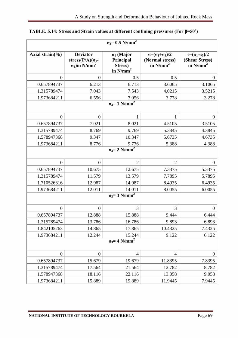
A Study on Strength and Deformation Behaviour of Jointed Rock Mass
NATIONAL INSTITUTE OF TECHNOLOGY ROURKELA Page 69
TABLE. 5.14: Stress and Strain values at different confining pressures (For β=50˚)
σ3= 0.5 N/mm2
Axial strain(%) Deviator
stress(P/A)(σ1-
σ3)in N/mm2
σ1 (Major
Principal
Stress)
in N/mm2
σ=(σ1+σ3)/2
(Normal stress)
in N/mm2
τ=(σ1-σ3)/2
(Shear Stress)
in N/mm2
0 0 0.5 0.5 0
0.657894737 6.213 6.713 3.6065 3.1065
1.315789474 7.043 7.543 4.0215 3.5215
1.973684211 6.556 7.056 3.778 3.278
σ3= 1 N/mm2
0 0 1 1 0
0.657894737 7.021 8.021 4.5105 3.5105
1.315789474 8.769 9.769 5.3845 4.3845
1.578947368 9.347 10.347 5.6735 4.6735
1.973684211 8.776 9.776 5.388 4.388
σ3= 2 N/mm2
0 0 2 2 0
0.657894737 10.675 12.675 7.3375 5.3375
1.315789474 11.579 13.579 7.7895 5.7895
1.710526316 12.987 14.987 8.4935 6.4935
1.973684211 12.011 14.011 8.0055 6.0055
σ3= 3 N/mm2
0 0 3 3 0
0.657894737 12.888 15.888 9.444 6.444
1.315789474 13.786 16.786 9.893 6.893
1.842105263 14.865 17.865 10.4325 7.4325
1.973684211 12.244 15.244 9.122 6.122
σ3= 4 N/mm2
0 0 4 4 0
0.657894737 15.679 19.679 11.8395 7.8395
1.315789474 17.564 21.564 12.782 8.782
1.578947368 18.116 22.116 13.058 9.058
1.973684211 15.889 19.889 11.9445 7.9445

A Study on Strength and Deformation Behaviour of Jointed Rock Mass
NATIONAL INSTITUTE OF TECHNOLOGY ROURKELA Page 70
Fig. 5.33: Normal Stress(MPa) Vs Shear Stress(MPa) at different confining pressures
Fig. 5.34: Axial strain(%) Vs Deviator stress(MPa) at different confining pressures
0
1
2
3
4
5
6
7
8
9
10
0 2 4 6 8 10 12 14
She
ar S
tre
ss(M
Pa)
Normal Stress(MPa)
for 0.5 MPa
for 1 MPa
for 2 MPa
for 3 MPa
for 4 MPa
0
2
4
6
8
10
12
14
16
18
20
0 0.5 1 1.5 2 2.5
Dev
iato
r st
ress
(MP
a)
Axial strain(%)
for 0.5 MPa
for 1 MPa
for 2 MPa
for 3 MPa
for 4 MPa

A Study on Strength and Deformation Behaviour of Jointed Rock Mass
NATIONAL INSTITUTE OF TECHNOLOGY ROURKELA Page 71
Fig. 5.35: σcj/σ3 Vs σdj/σ3 at different confining pressures(for jointed specimens i.e.,1-J-
50˚),where αj(50) and Bj(50) are material constants
y = 0.6904x + 3.4391 R² = 0.9912
1
10
100
1 10 100
σd
j/σ
3
σcj/σ3
αj(50)
= 0.6904
Bj(50)
= 3.4391

A Study on Strength and Deformation Behaviour of Jointed Rock Mass
NATIONAL INSTITUTE OF TECHNOLOGY ROURKELA Page 72
TABLE. 5.15: Stress and Strain values at different confining pressures (For β=60˚)
σ3= 0.5 N/mm2
Axial strain(%) Deviator
stress(P/A)(σ1-
σ3)in N/mm2
σ1 (Major
Principal
Stress)
in N/mm2
σ=(σ1+σ3)/2
(Normal stress)
in N/mm2
τ=(σ1-σ3)/2
(Shear Stress)
in N/mm2
0 0 0.5 0.5 0
0.657894737 6.545 7.045 3.7725 3.2725
1.315789474 7.434 7.934 4.217 3.717
1.842105263 8.134 8.634 4.567 4.067
2.236842105 7.006 7.506 4.003 3.503
σ3= 1 N/mm2
0 0 1 1 0
0.657894737 8.326 9.326 5.163 4.163
1.315789474 9.786 10.786 5.893 4.893
1.842105263 10.676 11.676 6.338 5.338
2.105263158 9.882 10.882 5.941 4.941
σ3= 2 N/mm2
0 0 2 2 0
0.657894737 11.266 13.266 7.633 5.633
1.315789474 12.657 14.657 8.3285 6.3285
1.710526316 13.478 15.478 8.739 6.739
1.973684211 13.011 15.011 8.5055 6.5055
σ3= 3 N/mm2
0 0 3 3 0
0.657894737 12.864 15.864 9.432 6.432
1.315789474 14.238 17.238 10.119 7.119
1.710526316 15.254 18.254 10.627 7.627
1.973684211 14.544 17.544 10.272 7.272
σ3= 4 N/mm2
0 0 4 4 0
0.657894737 14.559 18.559 11.2795 7.2795
1.315789474 16.453 20.453 12.2265 8.2265
1.973684211 17.347 21.347 12.6735 8.6735
2.105263158 18.322 22.322 13.161 9.161
2.631578947 15.408 19.408 11.704 7.704

A Study on Strength and Deformation Behaviour of Jointed Rock Mass
NATIONAL INSTITUTE OF TECHNOLOGY ROURKELA Page 73
0
2
4
6
8
10
12
14
16
18
20
0 0.5 1 1.5 2 2.5 3
Dev
iato
r st
ress
(MP
a)
Axial strain(%)
for 0.5 MPa
for 1 MPa
for 2 MPa
for 3 MPa
for 4 MPa
Fig. 5.36: Normal Stress(MPa) Vs Shear Stress(MPa) at different confining pressures
Fig. 5.37: Axial strain(%) Vs Deviator stress(MPa) at different confining pressures
0
1
2
3
4
5
6
7
8
9
10
0 2 4 6 8 10 12 14
Shea
r St
ress
(MP
a)
Normal Stress(MPa)
for 0.5 MPa
for 1 MPa
for 2 MPa
for 3 MPa
for 4 MPa

A Study on Strength and Deformation Behaviour of Jointed Rock Mass
NATIONAL INSTITUTE OF TECHNOLOGY ROURKELA Page 74
Fig. 5.38: σcj/σ3 Vs σdj/σ3 at different confining pressures(for jointed specimens i.e.,1-J-
60˚),where αj(60) and Bj(60) are material constants
y = 0.7697x + 3.1882 R² = 0.9899
1
10
100
1 10 100
σd
j/σ
3
σcj/σ3
αj(60)
= 0.7697
Bj(60)
= 3.1882

A Study on Strength and Deformation Behaviour of Jointed Rock Mass
NATIONAL INSTITUTE OF TECHNOLOGY ROURKELA Page 75
TABLE. 5.16 Stress and Strain values at different confining pressures (For β=70˚)
σ3= 1 N/mm2
Axial strain(%) Deviator
stress(P/A)(σ1-
σ3)in N/mm2
σ1 (Major
Principal
Stress)
in N/mm2
σ=(σ1+σ3)/2
(Normal stress)
in N/mm2
τ=(σ1-σ3)/2
(Shear Stress)
in N/mm2
0 0 1 1 0
0.657894737 8.552 9.552 5.276 4.276
1.315789474 9.426 10.426 5.713 4.713
1.578947368 10.412 11.412 6.206 5.206
1.973684211 9.128 10.128 5.564 4.564
σ3= 2 N/mm2
0 0 2 2 0
0.657894737 13.124 15.124 8.562 6.562
1.315789474 13.486 15.486 8.743 6.743
1.973684211 12.446 14.446 8.223 6.223
σ3= 3 N/mm2
0 0 3 3 0
0.657894737 13.236 16.236 9.618 6.618
1.315789474 14.886 17.886 10.443 7.443
1.710526316 15.847 18.847 10.9235 7.9235
1.973684211 14.008 17.008 10.004 7.004
σ3= 4 N/mm2
0 0 4 4 0
0.657894737 14.122 18.122 11.061 7.061
1.315789474 15.468 19.468 11.734 7.734
1.710526316 17.684 21.684 12.842 8.842
1.973684211 15.065 19.065 11.5325 7.5325
σ3= 5 N/mm2
0 0 5 5 0
0.657894737 14.544 19.544 12.272 7.272
1.315789474 16.654 21.654 13.327 8.327
1.447368421 18.148 23.148 14.074 9.074
1.973684211 16.222 21.222 13.111 8.111

A Study on Strength and Deformation Behaviour of Jointed Rock Mass
NATIONAL INSTITUTE OF TECHNOLOGY ROURKELA Page 76
Fig. 5.39: Normal Stress(MPa) Vs Shear Stress(MPa) at different confining pressures
Fig. 5.40: Axial strain(%) Vs Deviator stress(MPa) at different confining pressures
0
1
2
3
4
5
6
7
8
9
10
0 2 4 6 8 10 12 14 16
She
ar S
tre
ss(M
Pa)
Normal Stress(MPa)
for 1 MPa
for 2 MPa
for 3 MPa
for 4 MPa
for 5 MPa
0
2
4
6
8
10
12
14
16
18
20
0 0.5 1 1.5 2 2.5
Dev
iato
r st
ress
(MP
a)
Axial strain(%)
for 1 MPa
for 2 MPa
for 3 MPa
for 4 MPa
for 5 MPa
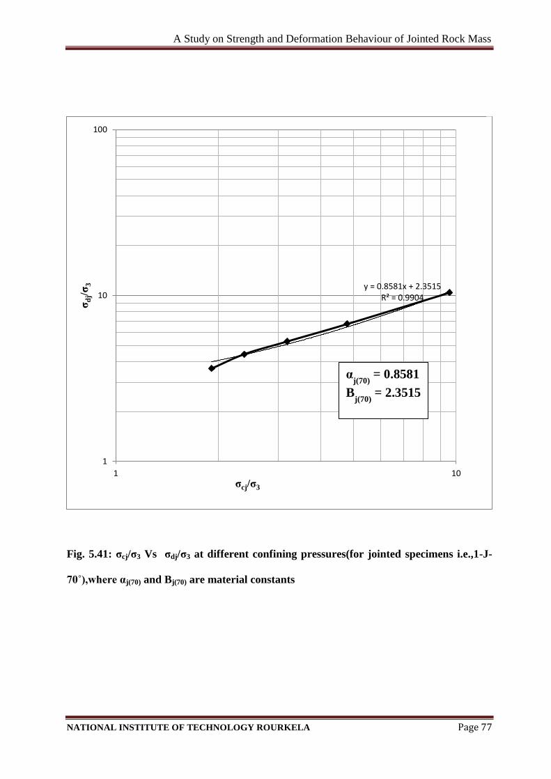
A Study on Strength and Deformation Behaviour of Jointed Rock Mass
NATIONAL INSTITUTE OF TECHNOLOGY ROURKELA Page 77
Fig. 5.41: σcj/σ3 Vs σdj/σ3 at different confining pressures(for jointed specimens i.e.,1-J-
70˚),where αj(70) and Bj(70) are material constants
y = 0.8581x + 2.3515 R² = 0.9904
1
10
100
1 10
σd
j/σ
3
σcj/σ3
αj(70)
= 0.8581
Bj(70)
= 2.3515

A Study on Strength and Deformation Behaviour of Jointed Rock Mass
NATIONAL INSTITUTE OF TECHNOLOGY ROURKELA Page 78
TABLE. 5.17: Stress and Strain values at different confining pressures (For β=80˚)
σ3= 1 N/mm2
Axial strain(%) Deviator
stress(P/A)(σ1-
σ3)in N/mm2
σ1 (Major
Principal
Stress)
in N/mm2
σ=(σ1+σ3)/2
(Normal stress)
in N/mm2
τ=(σ1-σ3)/2
(Shear Stress)
in N/mm2
0 0 1 1 0
0.657894737 9.479 10.479 5.7395 4.7395
1.315789474 10.004 11.004 6.002 5.002
1.842105263 10.466 11.466 6.233 5.233
1.973684211 9.222 10.222 5.611 4.611
σ3= 2 N/mm2
0 0 2 2 0
0.657894737 12.688 14.688 8.344 6.344
1.315789474 13.432 15.432 8.716 6.716
1.578947368 13.872 15.872 8.936 6.936
1.973684211 12.444 14.444 8.222 6.222
σ3= 3 N/mm2
0 0 3 3 0
0.657894737 13.124 16.124 9.562 6.562
1.315789474 14.128 17.128 10.064 7.064
1.973684211 15.845 18.845 10.9225 7.9225
2.631578947 12.998 15.998 9.499 6.499
σ3= 4 N/mm2
0 0 4 4 0
0.657894737 13.257 17.257 10.6285 6.6285
1.315789474 14.453 18.453 11.2265 7.2265
1.842105263 16.898 20.898 12.449 8.449
1.973684211 13.242 17.242 10.621 6.621
σ3= 5 N/mm2
0 0 5 5 0
0.657894737 13.867 18.867 11.9335 6.9335
1.315789474 16.123 21.123 13.0615 8.0615
1.710526316 17.245 22.245 13.6225 8.6225
1.973684211 13.544 18.544 11.772 6.772

A Study on Strength and Deformation Behaviour of Jointed Rock Mass
NATIONAL INSTITUTE OF TECHNOLOGY ROURKELA Page 79
Fig. 5.42: Normal Stress(MPa) Vs Shear Stress(MPa) at different confining pressures
Fig. 5.43: Axial strain(%) Vs Deviator stress(MPa) at different confining pressures
0
1
2
3
4
5
6
7
8
9
10
0 2 4 6 8 10 12 14 16
Sh
ear
Str
ess(
MP
a)
Normal Stress(MPa)
for 1 MPa
for 2 MPa
for 3 MPa
for 4 MPa
for 5 MPa
0
2
4
6
8
10
12
14
16
18
20
0 0.5 1 1.5 2 2.5 3
Dev
iato
r st
ress
(MP
a)
Axial strain(%)
for 1 MPa
for 2 MPa
for 3 MPa
for 4 MPa
for 5 MPa

A Study on Strength and Deformation Behaviour of Jointed Rock Mass
NATIONAL INSTITUTE OF TECHNOLOGY ROURKELA Page 80
Fig. 5.44: σcj/σ3 Vs σdj/σ3 at different confining pressures(for jointed specimens i.e.,1-J-
80˚),where αj(80) and Bj(80) are material constants
y = 0.8691x + 2.19 R² = 0.9817
1
10
100
1 10
σd
j/σ
3
σcj/σ3
αj(80)
= 0.8691
Bj(80)
= 2.19

A Study on Strength and Deformation Behaviour of Jointed Rock Mass
NATIONAL INSTITUTE OF TECHNOLOGY ROURKELA Page 81
TABLE. 5.18: Stress and Strain values at different confining pressures (For β=90˚)
σ3= 1 N/mm2
Axial strain(%) Deviator
stress(P/A)(σ1-
σ3)in N/mm2
σ1 (Major
Principal Stress)
in N/mm2
σ=(σ1+σ3)/2
(Normal stress)
in N/mm2
τ=(σ1-σ3)/2
(Shear Stress)
in N/mm2
0 0 1 1 0
0.657894737 9.433 10.433 5.7165 4.7165
1.315789474 10.666 11.666 6.333 5.333
1.842105263 11.023 12.023 6.5115 5.5115
2.236842105 9.244 10.244 5.622 4.622
σ3= 2 N/mm2
0 0 2 2 0
0.657894737 12 14 8 6
1.315789474 12.432 14.432 8.216 6.216
1.842105263 13.123 15.123 8.5615 6.5615
2.5 12.087 14.087 8.0435 6.0435
σ3= 3 N/mm2
0 0 3 3 0
0.657894737 13.442 16.442 9.721 6.721
1.315789474 14.888 17.888 10.444 7.444
1.842105263 16.433 19.433 11.2165 8.2165
2.236842105 14.126 17.126 10.063 7.063
σ3= 4 N/mm2
0 0 4 4 0
0.657894737 13.542 17.542 10.771 6.771
1.315789474 16.087 20.087 12.0435 8.0435
1.842105263 17.922 21.922 12.961 8.961
2.236842105 14.554 18.554 11.277 7.277
σ3= 5 N/mm2
0 0 5 5 0
0.657894737 13.867 18.867 11.9335 6.9335
1.315789474 16.234 21.234 13.117 8.117
1.973684211 18 23 14 9
2.631578947 12.345 17.345 11.1725 6.1725

A Study on Strength and Deformation Behaviour of Jointed Rock Mass
NATIONAL INSTITUTE OF TECHNOLOGY ROURKELA Page 82
Fig. 5.45: Normal Stress(MPa) Vs Shear Stress(MPa) at different confining pressures
Fig. 5.46: Axial strain(%) Vs Deviator stress(MPa) at different confining pressures
0
1
2
3
4
5
6
7
8
9
10
0 2 4 6 8 10 12 14 16
Sh
ear
Str
ess(
MP
a)
Normal Stress(MPa)
for 1 MPa
for 2 MPa
for 3 MPa
for 4 MPa
for 5 MPa
0
2
4
6
8
10
12
14
16
18
20
0 0.5 1 1.5 2 2.5 3
Dev
iato
r st
ress
(MP
a)
Axial strain(%)
for 1 MPa
for 2 MPa
for 3 MPa
for 4 MPa
for 5 MPa

A Study on Strength and Deformation Behaviour of Jointed Rock Mass
NATIONAL INSTITUTE OF TECHNOLOGY ROURKELA Page 83
Fig. 5.47: σcj/σ3 Vs σdj/σ3 at different confining pressures(for jointed specimens i.e.,1-J-
90˚),where αj(90) and Bj(90) are material constants
y = 0.8901x + 2.162 R² = 0.9925
1
10
100
1 10 100
σd
j/σ
3
σcj/σ3
αj(90)
= 0.8901
Bj(90)
= 2.162

A Study on Strength and Deformation Behaviour of Jointed Rock Mass
NATIONAL INSTITUTE OF TECHNOLOGY ROURKELA Page 84
Fig. 5.48: Joint orientation(β˚) vs Failure strength in MPa(σ1), for different confining
pressures
0
5
10
15
20
25
0 10 20 30 40 50 60 70 80 90 100
Fail
ure
str
ength
in
MP
a(σ
1)
Joint orientation(β˚)
for 0.5 MPa
for 1 MPa
for 2 MPa
for 3 MPa
for 4 MPa
for 5 MPa

A Study on Strength and Deformation Behaviour of Jointed Rock Mass
NATIONAL INSTITUTE OF TECHNOLOGY ROURKELA Page 85
CONCLUSIONS
On the basis of present experimental study on the intact and jointed specimen of plaster of
Paris the following conclusions are drawn:
1. The Plaster of Paris tested contained 22% quartz, 24% calcite, 43% mica and 11%
cementing materials.
2. The uniaxial compressive strength and Elastic modulus (Eti) of intact specimen of
plaster of Paris is found to be 11.24Mpa and 0.422 * Mpa respectively. Hence as
per ISRM (1979) classification of intact rocks, the plaster of paris tested in this study is
classified as low strength rock. And according to Deere and Miller (1966) classification
as EL depicting very low strength and low modulus ratio.
3. The following empirical relationship given by Arora (1987) have been used for
predicting the strength and elastic modulus of jointed rocks which is almost matching
with that of the present experimental strength and elastic modulus values.
σcr= and Er=
where, σcr=σcj/σci, Er =Ej / Ei , Jf=Jn/(n. r),
Jn = number of joints per meter depth;
n = inclination parameter depending on the orientation of the joint ;
r = roughness parameter depending on the joint condition;
σcj = uniaxial compressive strength of jointed rock;
σci = uniaxial strength of intact rock;
Ej =is the tangent modulus of jointed rock ;
.Ei =is the tangent modulus of intact rock

A Study on Strength and Deformation Behaviour of Jointed Rock Mass
NATIONAL INSTITUTE OF TECHNOLOGY ROURKELA Page 86
4. The strength of jointed specimen depends on the joint orientation β with respect to the
direction of major principal stress. The strength at β =30º is found to be minimum and
the strength at β= 90º is found to be maximum.
5. As the number of joints increases, the uniaxial compressive strength decreases.
6. The compressive strength is more when the double joints are made at angle of
orientation at 60º – 60º to than at 90 º - 90º.
7. The values of Modulus ratio (Er) also depends on the joint orientation β. The modulus
ratio is least at 30º.
8. For the intact specimens as well as all the single jointed specimens varying from 0˚ to
90˚, the response curves of triaxial compression test i.e., Normal Stress Vs Shear Stress
curves are almost similar in nature. With increase in Confining Pressure, the Normal
Stress as well as Shear stress increases and also both are directly proportional to each
other.
9. For all the specimens (intact and single jointed), it has been proved that, with increase
in confining pressure the failure strength also increases.

A Study on Strength and Deformation Behaviour of Jointed Rock Mass
NATIONAL INSTITUTE OF TECHNOLOGY ROURKELA Page 87
10. For intact specimens of Plaster Of Paris, the material constants, αi and Bi are found as
0.892 and 2.237 respectively, where
(σ1-σ3)/σ3 = Bj(σcj/σ3)α
j ; αj = αi (σcj/σ3)0.5
;
σcj= σci ; Bj= Bi/0.13
Where, σ1 and σ3 = major and minor principal stresses; σci = Uniaxial Compressive Strength of
intact specimens; αi = the slope of the plot between (σ1-σ3)/σ3 and σci/σ3, for most intact rocks
its mean value is 0.8; and Bi = a material constant, equal to (σ1-σ3)/σ3 when σci/σ3 = 1. The
value of Bi varies from 1.8 to 3.0 for argillaceous, arenaceous, chemical and igneous rocks. σcj
= Uniaxial Compressive Strength at an orientation; αj and Bj = values of α and B at the
orientation under consideration.
11. For the single jointed specimens, at each orientations i.e., from 0˚ to 90˚, the material
constants αj and Bj are found out and are represented in the respective figures. And also
it has been found that with increase in the value of joint orientation(β), the value of αj
increases whereas the value of Bj decreases for most cases.

A Study on Strength and Deformation Behaviour of Jointed Rock Mass
NATIONAL INSTITUTE OF TECHNOLOGY ROURKELA Page 88
SCOPE OF FUTURE WORK:
1. The effect of temperature, confining pressure and rate of loading on the strength
characteristics can be studied.
2. Studies can be made by introducing multiple joints in varying orientation.
3. Strength and deformation behaviour of jointed specimens can be studied under triaxial
conditions for the samples with more than one number of joints.
4. Strength and deformation behaviour of jointed specimens under triaxial conditions can be
studied with gouge filled joints.
5. Prediction of strength and deformation behavior of specimens with any arbitrary orientation
and at any number of joints can be done by using Artificial Neural Network with the help of
these datas as well as datas from the literature also can be taken.
6. Numerical models can be developed by using different theories and the results can be
compared with the Experimental results to reach at the best possible Numerical Model.
7. Different Softwares can be used to analyse the Experimental results.

A Study on Strength and Deformation Behaviour of Jointed Rock Mass
NATIONAL INSTITUTE OF TECHNOLOGY ROURKELA Page 89
REFERENCES
1. Arora, V. K. ( 1987). "Strength and deformation behavior of jointed rocks." PhD thesis,
IIT Delhi, India.
2. Barton, N. (1988). Rock Mass Classification and Tunnel Reinforcement Selection using
the Q-System. Rock Classification Systems for Engineering Purposes, ed. Kirkaldie, L.,
ASTM STP 984, pp. 59-84.
3. Barton, N. and Bandis, S. (1990). Review of predictive capabilities of JRC-JCS model
in engineering practice, Proc. Int. Conf. on Rock Joints, Rotterdam, Balkema, pp. 603-
610.
4. Bieniawski, Z.T. (1973). Engineering classification of jointed rock masses, J.S. Afr.
Inst. Min. Metall., Vol. 15, pp. 335-344
5. Bieniawski, Z. T. ( 1979). The geomechanics classification in rock engineering
application, Proc. 4th Int. Cong. Rock Mech., ISRM, Montreux, Vol. 2, pp. 51-58.
6. Brown, E. T. (1970). "Strength of models of rock with intermittent joints." J. Soil
Mech. Found. Div., 96(6), 1935-1949.
7. Brown. E. T., and Trollope, D. H. (1970). "Strength of model of jointed rock." J. Soil
Mech. Found. Div., 96(2), 685-704.
8. Deere, D.U. and Deere, D.W. (1988). The Rock Quality Designation (RQD) Index in
Practice, Rock Classification Systems for Engineering Purposes, (ed. L. Kirkaldie),
ASTM Special Publication 984, pp. 91-101.

A Study on Strength and Deformation Behaviour of Jointed Rock Mass
NATIONAL INSTITUTE OF TECHNOLOGY ROURKELA Page 90
9. Einstein, H. H., Nelson, R. A., Bruhn. R. W., and Hirschfeld, R. C.,(1970). "Model
studies of jointed rock behaviour." Proc., Ilth Symp. of Rock Mechanics, Berkeley,
Calif., 83-103.
10. Einstein, H. H., and Hirschfeld, R. C. (1973). "Model studies in mechanics of jointed
rocks." J. SIJiI Mech. Found. Div.. 99(3), 229-248.
11. Goldstein, M., Goosev, B., Pyrogovsky, Tulinov, R., and Turovskaya A. (1966).
"Investigations of mechanical properties of cracked rock." Proc., 1st Congress of
Society of Rock Mechanics, Lisbon, I, 521-524.
12. Goodman, Richard E, Intoduction to Rock Mechanics. New york, John Wiley, 1980
13. Gerrard, C. M. ( 1982). Elastic models of rock masses having one, two and three sets of
joints, Int. J. Rock Mech. Min. Sci. & Geomech. Abstr.,Vol.19, pp 5-23.
14. Hayashi, M., (1966). "Strength and dilatancy of brittle jointedmass.The extreme
stochastic and anisotropic failure mechanism." Proc., 1 st Int. Congress on Rock
Mechanics, Libson, I, 295-302.
15. Hoek, E. and Brown, E. T .( 1997). Practical estimates of rock mass strength, Int J.
Rock. Mech. Min. Sci., V 01. 34, No.8, pp. 1165-1186.
16. I.S. 11229 – 1985, Specifications for shear box for testing of soils.
17. I.S. 2720 (part XIII) – 1972, Determination of shear strength parameters from direct
shear test.
18. Jaeger C., Fundamentals of Rock Mechanics. London, Chapman and Hall, 1969.

A Study on Strength and Deformation Behaviour of Jointed Rock Mass
NATIONAL INSTITUTE OF TECHNOLOGY ROURKELA Page 91
19. Laboratory testing of rocks manual
20. Lama, R. D. (1974). "Uniaxial compressive strength of jointed rock." Institute of soil
mechanics and rock mechanics, P-Muller Festschrift.ed., Karlsruhe,Germany, 67- 77.
21. Lama, R. D. (1974). "Uniaxial compressive strength of jointed rock." Institute of soil
mechanics and rock mechanics, P-Muller Festschrift.ed., Karlsruhe,Germany, 67- 77.
22. Ramamurthy,T. (1994). "Strength and modulus responses of anisotropic rocks." Rock
Eng.. 1(13), 313-329
23. Roy, N. (1993). "Engineering behavior of rock masses through study of jointed
models." PhD thesis, Indian Institute of Technology, Delhi,India.
24. Shahin, M.A., Jaksa, M.B. and Maier, H.R. (2000). “Predicting the settlement of
shallow foundations on cohesion less soils using back-propagation neural networks”
Research.report No. R 167, Dept. of Civil and Envi.Eng.,University of Adelaide,
Australia
25. Simon Hilykin (2001) Neural Networks (A Comprehensive Foundation) Addison
Wesley Longrnan (Singapore) Pte. Ltd, Indian Branch Delhi.
26. Sitharam, T.G., Sridevi, J. and Shimizu, N. (2001). Practical equivalent continuum
characterization of jointed rock masses, International Journal of Rock Mechanics and
Mining Sciences, Vol. 38, pp. 437-448.
27. Sridevi, J. (2000). “Numerical modeling of jointed rock mass”, Ph.D. Thesis, Indian
Institute of Science, Bangalore, India.

A Study on Strength and Deformation Behaviour of Jointed Rock Mass
NATIONAL INSTITUTE OF TECHNOLOGY ROURKELA Page 92
28. Sridevi, J. and Sitharam, T .G .(2000). Analysis of Strength and Moduli of Jointed
Rocks, Int. J. Geotech. Geolog. Eng., Vol. 18, pp.1-19.
29. Sridevi, J., Sitharam, T.G. and Chandrashekar, H.M. (2000) Simulation of jointed rock
mass behavior using finite element method, Vol. 6, No, 2 pp. 113- 132
30. Sridevi, J. and Sitharam, T .G .(2003). Characterization of Strength and Deformation of
Jointed Rock Mass Based on Statistical Analysis. International journal of
Geomechanics ASCE 1 September.(43-54).
31. Terminology, ISRM, 1975
32. T G. SITHARAM, K ET. Al (2001).]ntelligent Prediction of Elastic Properties of
Jointed Rocks, J. of Rock Mech. & Tunneling Tech. Vol. 9.
33. Varadarajan, A., Sharma, K.G., Desai, C.S. and Hashemi, M. (2001) Analysis of a
powerhouse cavern in the Himalayas, Int. J. Geomech., Vol. I, No.1, pp.109-127.
34. Yaji, R. K. (1984). "Shear strength and deformation of jointed rocks."PhD thesis,
Indian Institute of Technology, Delhi, India.
35. Yegnanarayana, B. (1999). Artificial Neural Networks, Prentice-l-Hall of India private
Limited, New Delhi, India.
36. Zienkiewicz, O.C., Kelly, D.W. and Bettess, P. (1977). The coupling of the finite
element method and boundary solution procedures, International journal for numerical
methods in engineering, Vol. 11, pp. 355- 375.
37. Zurada, J .M. ( 1997). Introduction to artificial neural systems, Jaico Publishing House,
Mumbai, India.