A STUDY OF ADAPTIVE BEAMFORMING TECHNIQUES USING SMART ANTENNA FOR

MOBILE COMMUNICATION

A THESIS SUBMITTED IN PARTIAL FULFILLMENT

OF THE REQUIREMENTS FOR THE DEGREE OF

Master of Technology in

Electrical Engineering

By

Shankar Ram

Department of Electrical Engineering

National Institute of Technology

Rourkela

2007

A STUDY OF ADAPTIVE BEAMFORMING TECHNIQUES USING SMART ANTENNA FOR

MOBILE COMMUNICATION A THESIS SUBMITTED IN PARTIAL FULFILLMENT

OF THE REQUIREMENTS FOR THE DEGREE OF

Master of Technology in

Electrical Engineering

By

Shankar Ram

Under the Guidance of

Prof. Susmita Das

Department of Electrical Engineering

National Institute of Technology

Rourkela

2007

National Institute of Technology

Rourkela

CERTIFICATE

This is to certify that the thesis entitled, “A Study of Adaptive Beamforming

Techniques Using Smart Antenna for Mobile Communication” submitted by Sri

Shankar Ram in partial fulfillment of the requirements for the award of MASTER of

Technology Degree in Electrical Engineering with specialization in “Electronics System

and Communication” at the National Institute of Technology, Rourkela (Deemed

University) is an authentic work carried out by him under my supervision and guidance.

To the best of my knowledge, the matter embodied in the thesis has not been submitted to

any other University/ Institute for the award of any degree or diploma.

Date: Prof. Susmita Das

Dept. of Electrical Engineering. National Institute of Technology

Rourkela - 769008

Acknowledgement

I would like to express my deep sense of respect and gratitude toward my supervisor Dr.

Susmita Das, who not only guided the academic project work but also stood as a teacher and

philosopher in realizing the imagination in pragmatic way. I want to thank her for introducing me

in the field of the Smart Antenna for wireless communication. Her presence and optimism have

provided an invaluable influence on my career and outlook for the future. I consider it as my

good fortune to have got an opportunity to work with such a wonderful person.

I express my gratitude to Dr P.K. Nanda, Professor and Head, Department of Electrical

Engineering, faculty member and staff of Department of Electrical Engineering for extending all

possible help in carrying out the dissertation work directly or indirectly. They have been great

source of inspiration to me and I thank them from bottom of my heart. I would like to

acknowledge my institute, National Institute of Technology, Rourkela, for providing good

facilities to complete my thesis work.

I would also like to take this opportunity to acknowledge my friends for their support and

encouragement. Without them, it would have been very difficult for me to complete my thesis

work.

I am especially indebted to my parents for their love, sacrifice and support. They are my

teachers after I came to this world and have set great example for me about how to live, study

and work.

At last, I would like to give thanks to God since He has given me wisdom, health and all the

necessities that I need for all these years.

Shankar Ram

i

Contents Acknowledgement…………………………………………………………………………i

Abstract…………………………………………………………………………………...iv

List of Figure……………………………………………………………………………..vi

Chapter 1 Introduction………………………………………………………………….1

Chapter 2- Antennas and Antenna Systems……………………………………………9

2.1 A Useful Analogy for Adaptive Smart Antenna………………………………...10

2.2 Antennas………………………………………………………………………....10

2.2.1 Omni Directional Antenna………………………………………………………..10

2.2.2 Directional Antennas……………………………………………………………...11

2.3 Antenna Systems………………………………………………………...............12

2.3.1 Sectorized Systems……………………………………………………………….12

2.3.2 Diversity Systems………………………………………………………………...13

2.3.3 Smart………………………………………………………………………14

Chapter 3- Brief Overview of Smart Antenna System…………………………….15

3.1 How Many Types of Smart Antenna Systems Are There?....................................16

3.1.1 What Are Switched Beam Antennas?.......................................................................16

3.1.2 What Are Adaptive Array Antennas?.......................................................................17

3.2 What Do They Look Like?.....................................................................................17

3.3 The Goals of the Smart Antenna System…………………………………………18

3.4 Smart Antenna Drawbacks……………………………………………………….19

Chapter 4- Multipath path and co-channel interference…………………………….20

4.1 A Useful Analogy for Signal Propagation………………………………………..21

4.2 Multipath………………………………………………………………………….21

4.3 Problems Associated with Multipath……………………………………………..21

Chapter 5- Architecture of Smart Antenna System….………………………………25

5.1 How Do Smart Antenna Systems Work?...............................................................26

5.1.1 Listening to the Cell (Uplink Processing)…………………………………………26

ii

5.1.2 Speaking to the Users (Downlink Processing)……………………………………..26

5.2 Switched Beam Systems………………………………………………………….27

5.3 Adaptive Antenna Approach……………………………………………………..28

5.4 Relative Benefits/Tradeoffs of Switched Beam and Adaptive Array

Systems…………………………………………………………………………………..28

Chapter 6- Basics of Smart Antenna Approach………………………………………31

6.1 Antenna Array (Smart Antenna)………………………………………………....32

6.2 Conventional Beam-forming…………………………………………………….33

6.3 Effect of the element spacing on the beam pattern ……………………………...34

6.4 Effect of the array aperture on the beam pattern…………………………………35

6.5 Adaptive Beam-forming Algorithm……………………………………………...36

6.5.1 Sample Matrix Inversion…………………………………………………………..37

6.5.2 Least Mean Square Algorithm….………………………………………………….39

6.5.3 Constant Modulus Algorithm………………………………………………………42

6.5.4. Least Square Constant Modulus..………………………………………………….45

6.5.5 Recursive Least Square Algorithm.. ……………………………………………….48

Chapter 7- Comparison of Beamforming Algorithms ………………….…………....52

7.1 Comparison of Algorithms……….. ……………………………………………………...53

Chapter 8- Conclusion and Scope for Future Work…………………………………57 8.1 Conclusion..……………………………………………………………………….58

8.2 Scope of Future Work…………………………………………………………………….59

Reference..………………………………………………………………………………60

iii

Abstract

Mobile radio network with cellular structure demand high spectral efficiency for

minimizing number of connections in a given bandwidth. One of the promising technologies is

the use of “Smart Antenna”. A smart antenna is actually combination of an array of individual

antenna elements and dedicated signal processing algorithm. Such system can distinguish signal

combinations arriving from different directions and subsequently increase the received power

from the desired user. Wireless systems that enable higher data rates and higher capacities have

become the need of hour. Smart antenna technology offer significantly improved solution to

reduce interference level and improve system capacity. With this technology, each user’s signal

is transmitted and received by the base station only in the direction of that particular user. Smart

antenna technology attempts to address this problem via advanced signal processing technology

called beam-forming. The advent of powerful low-cost digital signal processors (DSPs), general-

purpose processors (and ASICs), as well as innovative software-based signal-processing

techniques (algorithms) have made intelligent antennas practical for cellular communications

systems and makes it a promising new technology. Through adaptive beam-forming, a base

station can form narrower beam toward user and nulls toward interfering users.

In this thesis, both the block adaptive and sample-by-sample methods are used to update

weights of the smart antenna. Block adaptive beam-former employs a block of data to estimate

the optimum weight vector and is known as sample matrix inversion (SMI) algorithm. The

sample-by-sample method updates the weight vector with each sample. Various sample-by-

sample methods, attempted in the present study are least mean square (LMS) algorithm, constant

modulus algorithm (CMA), least square constant modulus algorithm(LS-CMA) and recursive

least square (RLS) algorithm. In the presence of two interfering signals and noise, both

amplitude and phase comparison between desired signal and estimated output, beam patterns of

the smart antennas and learning characteristics of the above mentioned algorithms are compared

and analyzed. The recursive least square algorithm has the faster convergence rate; however

this improvement is achieved at the expense of increase in computational complexity.

Smart antennas technology suggested in this present work offers a significantly improved

solution to reduce interference levels and improve the system capacity. With this novel

technology, each user’s signal is transmitted and received by the base station only in the

direction of that particular user. This drastically reduces the overall interference in the system.

Further through adaptive beam forming, the base station can form narrower beams towards the

iv

desired user and nulls towards interfering users, considerably improving the signal-to-

interference-plus-noise ratio. It provides better range or coverage by focusing the energy sent out

into the cell, multi-path rejection by minimizing fading and other undesirable effects of multi-

path propagation.

v

List of Figure Chapter 1

1.1 Spectrum allocation in multiple cells with frequency reuse………………………………….3

1.2 Impact of smart antenna on wireless communication………………………………………...8

Chapter 2

2.1 Omni directional Antenna and Coverage Patterns….……………………………………….11

2.2 Directional Antenna and Coverage Pattern.…………………………………………………12

2.3 Sectorized Antenna and Coverage Patterns….………………………………………………13

2.4 Switched Diversity Coverage with Fading and Switched Diversity…...…………………….13

2.5 Combined Diversity Effective Coverage Pattern with Single Element and Combined

Diversity………………………………………………………………………………………….14

Chapter 3

3.1 Switched Beam System Coverage Patterns (Sectors)….…………………………………….16

3.2 Adaptive Array Coverage….………………………………………………………………...17

3.3 Different array geometries for smart antenna: a) Uniform linear array, b) Circular array, c)

Two dimensional grid array and d) Three dimensional grid array………………………………17

Chapter 4

4.1 The Effect of Multipath on a Mobile User….……………………………………………….21

4.2 Two Out-of-Phase Multipath Signals….…………………………………………………….22

4.3 A Representation of the Rayleigh Fade Effect on a User Signal…..………………………..22

4.4 Illustration of Phase Cancellation………….………………………………………………..23

4.5 Multipath: The Cause of Delay Spread…..………………………………………………….23

4.6 Illustration of Co channel Interference in a Typical Cellular Grid….………………………23

Chapter 5

5.1 Beam forming Lobes and Nulls that Switched Beam (Red) and Adaptive Array (Blue)

Systems might choose for Identical User Signals (Green Line) and Co channel Interferers

(Yellow Lines)…………………………………………………………………………………...27

5.2 Coverage Patterns for Switched Beam and Adaptive Array Antennas….…………………..28

5.3 Fully Adaptive Spatial Processing, Supporting Two Users on the Same Conventional

Channel Simultaneously in the Same Cell……………………………………………………….30

vi

Chapter 6

6.1 Adaptive Beam forming block diagram.…………………………………………………….33

6.2 Conventional beam former…….…………………………………………………………….33

6.3 A sample beam-pattern for a spatial matched filter for an N=16 element ULA and

φ = …………………………………………………………………………………………….34 °0

6.4 Beam-pattern for different element spacing λ/4, λ/2, λ, and 2λ respectively (equal size

aperture of 10λ with 40, 20, 10, and 5 elements respectively)…………………………………..35

6.5 Beam-pattern for different aperture sizes2λ, 4λ, 8λ, and 16λ respectively (common element

spacing of d= λ/2 with 4, 8, 16, and 32 elements respectively…………………………………..36

6.6 The beam-pattern of SMI adaptive beam-former for 8-elements ULA. The signal of interest

and two interfering signal are arriving at , and respectively. ………………….....39 °10 °− 35 °32

6.7 Comparison of the phase of desired signal and output for LMS…….………………………40

6.8 Comparison of the amplitude of desired signal and output for LMS….…………………….41

6.9 Performance curve for LMS algorithm ….………………………………………………….41

6.10 The beam-pattern of LMS algorithm adaptive beam-former for 8-elements ULA. The signal

of interest and two interfering signal are arriving at 35, 0 and -20 degree

respectively……………………………………………………………………………………....42

6.11 Comparison of the phase of desired signal and array output for CMA…….……………....43

6.12 Comparison of the amplitude of desired signal and array output for CMA………………..44

6.13 Performance curve for CMA……………………………………………………………….44

6.14 The beam-pattern of CMA adaptive beam-former for 8-elements ULA. The signal of

interest and two interfering signal are arriving at 35, 0 and -20 degree respectively.

……………………………………………………………………………………………………45

6.15 Comparison of the phase of desired signal and array output for LS-CMA………………...46

6.16 Comparison of the amplitude of desired signal and array output for LS-CMA…….47

6.17 Performance curve for LS-CMA algorithm………………………………………………...47

6.18 The beam-pattern of LS-CMA algorithm adaptive beam-former for 8-elements ULA. The

signal of interest and two interfering signal are arriving at 35, 0 and -20 degree respectively.

……………………………………………………………………………………………………48

6.19 Comparison of the phase of desired signal and array output for RLS……………………...49

6.20 Comparison of the amplitude of desired signal and array output for RLS…………………50

6.21 Performance curve for RLS algorithm……………………………………………………...50

vii

6.22 The beam-pattern of RLS algorithm adaptive beam-former for 8-elements ULA. The signal

of interest and two interfering signal are arriving at 35, 0 and -20 degree

respectively………………………………………………………………………………………51

Chapter 7

7.1 SMI adaptive beam-forming for 8-elements ULA. The signal of interest and two interfering

signal are arriving at , and respectively…………………………………………....53 °10 °− 35 °32

7.2 LMS adaptive beam-forming for 8-elements ULA and μ =0.05. The signal of interest and

two interfering signal are arriving at , and respectively. ………………………….54 °10 °− 35 °32

7.3 CMA adaptive beam-forming for 8-elements ULA and μ =0.05. . The signal of interest and

two interfering signal are arriving at , and respectively…………………………...54 °10 °− 35 °32

7.4 LS- CMA adaptive beam-forming for 8-elements ULA and μ =0.05. . The signal of interest

and two interfering signal are arriving at , and respectively……………………....55 °10 °− 35 °32

7.5 RLS adaptive beam-forming for 8-elements ULA, 1=λ and 004.0=δ . The signal of

interest and two interfering signal are arriving at , and respectively. …………….56 °10 °− 35 °32

viii

1

CHAPTER 1

INTRODUCTION

2

In the past decade, there has been a tremendous growth in the area of telecommunications.

As cellular phones and the high speed Internet become more and more popular, the demand for

faster and more efficient telecommunication systems has been skyrocketing. Both the increase in

the number of users and the increase in high data rate transfers from the Internet have produced a

huge increase in traffic. In order to handle this heavy traffic, the whole telecommunications

infrastructure has been transformed in the past several years. Thousands and thousands of optical

fibers were laid underground to allow high speed, wide bandwidth signal transfer. This has

solved most of the problems for land-based systems. However, more and more high-speed

services are now carried out in a mobile environment where data transfer is done through

wireless channels. Compared to the capacity of a fiber, the capacity of a wireless link is the

weakest part in the whole infrastructure. Many people have realized this and have tried different

methods to increase the bandwidth of the wireless channels.

Before going any further, let us explain how wireless communications systems work [1].

In most wireless communications systems, there are two major components - base stations and

the mobiles. The base station is located at the center of a coverage area called a ‘cell’ and the

mobiles can be anywhere within the cell. Communication then takes place between the base

station and the mobile through the wireless channel. A certain amount of spectrum is assigned to

a cell for signal transfer. This spectrum provides the media for the signals to be transmitted. With

a wider spectrum, more users can be served within a cell. To serve a large area, one can use a

high power base station to cover the whole area. but only a fixed amount of users can be served

in this way. So instead of having a single large cell, multiple cells with smaller size are usually

used to cover a large area. To avoid severe interference between cells, base stations that are

adjacent to each other are allocated different spectrum or channel groups. Also the output power

of the base station is maintained at a level so it is just enough to cover the whole area up to the

cell boundary. With this method, cells that are separated by a certain amount of distance can use

the same spectrum. This is true as long as the interference caused by surrounding co-channel

cells is within tolerable limits. Figure1.1. Shows one possible frequency reuse topology with a

cluster size of seven. In this frequency reuse scheme, each cell in the cluster has one-seventh of

the total spectrum, and the same spectrum is used in cells with the same label. With this cellular

reuse method, the same spectrum can now be reused over and over again and can be used to

cover an infinitely large area.

3

Fig.1.1. Spectrum allocation in multiple cells with frequency reuse

To allow simultaneous communication with multiple users within the same cell, the system has

to have methods to isolate the signals from each user. A typical method is to separate users by

frequency. In this kind of system, signals from each user are transmitted at different frequencies and

are separated by proper filtering.

By now, one should have a brief idea on how wireless communications systems function. So let

us explore some of the possibilities in improving the system performance. The easiest way is to use

more spectrum in each cell so that more users can be handled by the same base station, provided that

the user’s bandwidth remains unchanged, or more bandwidth can be assigned to each user so that

faster data transfer rates can be achieved through the wireless channel. Although this approach does

not require any changes in the system architecture, it is an impractical and expensive approach. This

is because there is limited spectrum allocated for wireless applications and it costs a lot of money for

the service providers to rent it. More spectrum is available at higher frequencies, but the cost of

building RF components that work at these frequency ranges becomes an issue. Another approach to

enhance the capacity and the performance of the system is to minimize the size of a cell so that each

serves a smaller area with the same amount of users, increasing overall density. This is a good

method and is used by most service providers to increase the system capacity. However, there is still

a limitation in how close co-channel cells can be put together. Besides, more base stations are

required to cover the same area, driving up the cost. The last approach is quite different from the

4

previous two. Instead of finding more spectrums to serve the same number of users, different

transmission techniques are used so that the system can serve more users with the same amount of

spectrum. Unlike the prior two approaches that do not require changes in the system design, this

method needs hardware customized to the transmission method. Although the base station is more

expensive, the additional cost is likely less than that of buying more spectrums. This system makes

better use of the available spectrum and has a higher spectral efficiency.

Many transmission methods have been developed in the past for wireless communications.

They vary from the very simple that support one user per channel to those that handle multiple

users per channel. Some access schemes that are commonly used in wireless communications are

listed below.

The simplest access scheme is called Frequency Division Multiple Access (FDMA). It is

widely used in many wireless applications like TV broadcast, radio broadcast, cellular system,

etc. In FDMA, signals from different users are transmitted with different frequencies just to

avoid interference. Each signal is isolated from others by passing the received signals through a

band pass filter. This method has been available for many decades and is used mainly in analog

systems. With the invention of digital technology, new methodologies became available in

designing communications systems and access schemes. The two most well known access

schemes that make use of the digital technology are Time Division Multiple Access (TDMA)

and Code Division Multiple Access (CDMA). Unlike FDMA, which can only support one user

per channel, both of these support multiple users per channel and increase the system capacity.

In TDMA systems, users are not just separated by frequency, but are separated both by

time and frequency. By doing so, multiple users can now share the same frequency channel by

having a different time slot. This kind of access scheme works well for voice communication.

Although a user is not transmitting or receiving during the whole communication, the signal

segments are carefully put together to reconstruct the original signal at the receiver with no

difference to a human ear. However, the data rate will be compromised in case of data

transmission with TDMA compared to other access schemes that do not require time sharing.

Unlike TDMA, which is still partly based on the FDMA concept, CDMA uses a totally

different concept. In CDMA, the signal from each user is spread across the entire channel by a

unique spreading code. The codes are chosen so that they are orthogonal to each other. They act

as the key to access the message in the transmitted signal. To retrieve a particular message at the

5

receiver, the corresponding code or key is used to extract the signal. To further illustrate how

the multiple access takes place, a simple analogy is used below to explain the process. In

CDMA, each code acts like a mask, which makes only the signal being transmitted with the same

mask visible but not signals with other masks. In an ideal situation, an infinite number of users

can be added to the same channel as long as the system can supply an uncorrelated code for each

signal. However, the orthogonal characteristics of the code diminish when they travel through

the wireless channel. This means that the masks are not perfect and do not give perfect isolation

from other signals. Leaking signals from other users now cause interference and noise in the

desired signal. More interference is received if more users are added to the channel, decreasing

the signal-to-interference plus noise ratio (SINR) of the desired signal. Since a certain amount of

SINR is required to ensure an acceptable signal quality, this interference in turn limits the system

capacity in the CDMA system. But if there is a method to minimize this co-channel interference,

the system capacity can obviously be increased in the CDMA system.

TDMA or CDMA systems can have 3 to 6 times the capacity of FDMA systems.

However, there is still a lot of room for improving system performance. It is always a challenge

to provide higher system capacity in the network to fulfill the growing demand. A lot of research

is being performed to look for methods to further improve system performance and the spectral

efficiency. One recent development in this area is a use of smart antenna with algorithm [2, 3],

also known as Space Division Multiple Access (SDMA) technology.

SDMA [4] is a totally different concept compared to TDMA and CDMA. It uses a

different technique to separate users. Instead of using time or code, users are now separated by

their spatial locations. Although SDMA may be new to commercial use, this is not the case for

military applications. In the past, similar systems were used to counter electronic jamming in

electronic warfare. It may not be as powerful as the one that is built in this project, but the basic

concept stays the same. It makes use of the fact that the jammer is usually located at a different

point to the desired communication partner. By adjusting the radiation pattern of the antenna

structure, the effect of the jammer can be reduced by placing a null in the direction of the

jammer. This was sometimes done in the past by manually changing the orientation of a highly

directional antenna. The same concept is now used in the commercial system. But instead of

eliminating jammers, the system is now used to reduce interference from co-channel users. Also,

6

no more hand-tuning is needed in the antenna since the radiation pattern can be manipulated by

software.

To implement an SDMA system, the most obvious difference in the system architecture

compared to regular systems is the antenna design. In a regular base station, the antenna is either

omni-directional or sectorized. To establish a connection between the base station and the

mobile, the transmitted signal is broadcast from the base station antenna. Its goal is to cover the

entire cell or sector so that the mobile can pick up the broadcast signal as long as it is within the

coverage area. However, this kind of signal transmission wastes a lot of energy due to the fact

that the mobile being addressed can only occupy one spot at a time. With broadcasting, most of

the power is radiated in other directions instead of traveling toward the desired user. Besides, the

broadcasting signal also causes undesired interference to other users located within the cell. If

there is a way to pinpoint a user within the cell so that the transmitting antenna aims toward the

desired user, less power will be needed to carry out the transmission. Also a lot of unnecessary

interference can be removed from the desired signal. This is the basic philosophy behind SDMA.

One may wonder, if this concept has been around for so many years and is so beneficial,

why has it only recently become popular. There is no simple answer to this question, but the

computation requirement in such a system plays a major role in hindering its implementation. As

mentioned earlier, in order for the system to have a flexible radiation pattern, some kind of

adaptation process has to be added to the system. There are different levels of intelligence

available and the kind of intelligence selected directly affects the performance of the system. In

the past, computational cost was large. The computation requirement needed to implement the

simplest algorithm could cost quite a lot of money. Also, there was no reason for the provider to

spend money on something that was not necessary at that time. Only recently has the demand for

system capacity gone up tremendously so that sophisticated multiple access schemes are now

economically viable.

In order to manipulate the radiation pattern of an antenna structure with software, multiple

antennas are required instead of a single antenna. Unlike a single antenna, which has a fixed

radiation pattern, the radiation pattern of an antenna array can be quite flexible. The flexibility

varies according to the algorithm being implemented in the system. The most straight forward

approach to generate a flexible radiation pattern is the switched lobe (SL) or the switched beam

technique where the antenna array contains a number of highly directional antennas. Each of the

7

antennas points in a slightly different direction. The system then analyzes the received signal

from each of the antennas and selects the one that has the best signal. A more intelligent

approach would be, instead of switching antennas, determine the direction of arrival (DoA) of

the signal. Once the DoA is obtained, the system uses the antenna array to form a highly

directional beam pointing toward the user. Both methods should provide some advantages over

the conventional system; however the benefit would be minimal if the signal suffers a lot of

angular spread where the signal arrives at many different directions in a multipath environment.

The situation would be even worse when no line-of-sight (LOS) is present between the user and

the base station.

To overcome the above shortcoming, a more advanced method was developed. This

method, usually called the optimum beam forming technique, fully utilizes the spatial diversity

present in the multipath channel so that a stronger received signal can be generated. With

optimum beam forming, signals received from multiple antennas are adjusted separately in both

amplitude and phase before being combined. By doing so, the system behaves as if it has

multiple adjustable radiation patterns. Each of the patterns is tuned to receive signals from a

single user. An adaptive algorithm is used at the base station so that the system has the ability to

determine the optimal radiation pattern for each user. As part of the training procedure, each of

the users transmits a short training sequence to the base station. The algorithm then makes use of

this information from a user by comparing each received signal to the original sequence to find

out the correct radiation pattern for that user. With this method, all received signals from each

antenna element are used and are optimally combined to enhance the desired signal and to cancel

unwanted interference. During the training process, a lot of number crunching is needed at the

base station. So it was not popular in the past due to the expensive cost of computation power.

However, intensive signal processing is no longer an issue with the availability of low cost,

extremely fast processors. Keep in mind that what actually happens in optimal beam forming is

more complicated than what is shown in the diagram. It is more complicated when interference

from other mobile occurs.

As mentioned earlier, SDMA provides a lot of benefits. For example, signals are now

radiated more directly toward the selected user. This increases the power efficiency and extends

the coverage area. Multipath fading is no longer an issue with a SDMA system. With multiple

antennas, each of them located at a different spot, the possibility of having a fade at all of the

8

antennas simultaneously is very small and can be ignored. Interference from other users is now

minimized. This improves the SINR of the received signal and therefore gives better signal

quality. It also provides another way of having multiple users on the same frequency channel

since signals originating from users at different locations are reduced after the signal combining.

This further increases the system capacity and also the spectral efficiency.

The development of a truly personal communication space will rely on the design of next-

generation wireless system which require adoption of smart antenna technique in order to

provide the expected beneficial impact on efficient use of the spectrum, minimization of the cost,

robust and transparent operation across multi-technology wireless network. Today, when

spectrally efficient solutions are increasingly a business imperative, these systems are providing

greater coverage area for each cell site, higher rejection of interference, data rate and substantial

capacity improvements as shown in fig1.2.

Fig.1.2. Impact of smart antenna on wireless communication

9

CHAPTER 2

ANTENNAS AND ANTENNA SYSTEMS

10

2.1 A Useful Analogy for Adaptive Smart Antenna

For an intuitive grasp of how an adaptive antenna system works, close your eyes and

converse with someone as they move about the room. You will notice that you can determine

their location without seeing them because of the following:

• You hear the speaker's signals through your two ears, your acoustic sensors.

• The voice arrives at each ear at a different time.

• Your brain, a specialized signal processor, does a large number of calculations to correlate

information and compute the location of the speaker.

Your brain also adds the strength of the signals from each ear together, so you perceive

sound in one chosen direction as being twice as loud as everything else.

Adaptive antenna systems [5] do the same thing, using antennas instead of ears. As a result,

8, 10, or 12 ears can be employed to help fine-tune and turn up signal information. Also, because

antennas both listen and talk, an adaptive antenna system can send signals back in the same

direction from which they came. This means that the antenna system cannot only hear 8 or 10 or

12 times louder but talk back more loudly and directly as well.

Going a step further, if additional speakers joined in, your internal signal processor could

also tune out unwanted noise (interference) and alternately focus on one conversation at a time.

Thus, advanced adaptive array systems have a similar ability to differentiate between desired and

undesired signals.

2.2 Antennas

Radio antennas couple electromagnetic energy from one medium (space) to another (e.g.,

wire, coaxial cable, or waveguide). Physical designs can vary greatly.

2.2.1 Omni Directional Antennas

Since the early days of wireless communications, there has been the simple dipole antenna,

which radiates and receives equally well in all directions. To find its users, this single-element

design broadcasts omni directionally in a pattern resembling ripples radiating outward in a pool

of water. While adequate for simple RF environments where no specific knowledge of the users'

11

whereabouts is available, this unfocused approach scatters signals, reaching desired users with

only a small percentage of the overall energy sent out into the environment.

Fig.2.1. Omni directional Antenna and Coverage Patterns

Given this limitation, omni directional strategies attempt to overcome environmental

challenges by simply boosting the power level of the signals broadcast. In a setting of numerous

users (and interferers), this makes a bad situation worse in that the signals that miss the intended

user become interference for those in the same or adjoining cells.

In uplink applications (user to base station), omni directional antennas offer no preferential

gain for the signals of served users. In other words, users have to shout over competing signal

energy. Also, this single-element approach cannot selectively reject signals interfering with those

of served users and has no spatial multi-path mitigation or equalization capabilities.

Omni directional strategies directly and adversely impact spectral efficiency, limiting

frequency reuse. These limitations force system designers and network planners to devise

increasingly sophisticated and costly remedies. In recent years, the limitations of broadcast

antenna technology on the quality, capacity, and coverage of wireless systems have prompted an

evolution in the fundamental design and role of the antenna in a wireless system.

2.2.2 Directional Antennas

A single antenna can also be constructed to have certain fixed preferential transmission and

reception directions [5]. As an alternative to the brute force method of adding new transmitter

sites, many conventional antenna towers today split, or sectaries cells. A 360° area is often split

into three 120° subdivisions, each of which is covered by a slightly less broadcast method of

transmission.

12

All else being equal, sector antennas provide increased gain over a restricted range of

azimuths as compared to an omni directional antenna. This is commonly referred to as antenna

element gain and should not be confused with the processing gains associated with smart antenna

systems. While sectaries antennas multiply the use of channels, they do not overcome the major

disadvantages of standard omni directional antenna broadcast such as co channel Interference.

Fig.2.2. Directional Antenna and Coverage Pattern

2.3 Antenna Systems

How can an antenna be made more intelligent? First, its physical design can be modified by

adding more elements. Second, the antenna can become an antenna system that can be designed

to shift signals before transmission at each of the successive elements so that the antenna has a

composite effect. This basic hardware and software concept is known as the phased array

antenna.

The following summarizes antenna developments in order of increasing benefits and

intelligence.

2.3.1 Sectorized Systems

Sectorized antenna systems [5] take a traditional cellular area and subdivide it into sectors

that are covered using directional antennas looking out from the same base station location.

Operationally, each sector is treated as a different cell, the range of which is greater than in the

omni directional case. Sector antennas increase the possible reuse of a frequency channel in such

cellular systems by reducing potential interference across the original cell, and they are widely

used for this purpose. As many as six sectors per cell have been used in practical service. When

combining more than one of these directional antennas, the base station can cover all directions.

13

Fig.2.3. Sectorized Antenna and Coverage Patterns

2.3.2 Diversity Systems

In the next step toward smart antennas, the diversity system [6] incorporates two antenna

elements at the base station, the slight physical separation (space diversity) of which has been

used historically to improve reception by counteracting the negative effects of multipath .

Diversity offers an improvement in the effective strength of the received signal by using

one of the following two methods:

• Switched diversity. Assuming that at least one antenna will be in a favorable location at a

given moment, this system continually switches between antennas (connects each of the

receiving channels to the best serving antenna) so as always to use the element with the largest

output. While reducing the negative effects of signal fading, they do not increase gain since only

one antenna is used at a time.

• Diversity combining. This approach [7] corrects the phase error in two multipath signals

and effectively combines the power of both signals to produce gain. Other diversity systems,

such as maximal ratio combining systems, combine the outputs of all the antennas to maximize

the ratio of combined received signal energy to noise.

Because macro cell-type base stations historically put out far more power on the downlink

(base station to user) than mobile terminals can generate on the reverse path, most diversity

antenna systems have evolved only to perform in uplink (user to base station).

Fig. 2.4. Switched Diversity Coverage with Fading and Switched Diversity

14

Fig2.5. Combined Diversity Effective Coverage Pattern with Single Element and Combined Diversity

Diversity antennas merely switch operation from one working element to another. Although

this approach mitigates severe multipath fading, its use of one element at a time offers no uplink

gain improvement over any other single element approach. In high-interference environments,

the simple strategy of locking onto the strongest signal or extracting maximum signal power

from the antennas is clearly inappropriate and can result in crystal-clear reception of an interferer

rather than the desired signal.

The need to transmit to numerous users more efficiently without compounding the

interference problem led to the next step of the evolution antenna systems that intelligently

integrate the simultaneous operation of diversity antenna elements.

2.3.3 Smart

The concept of using multiple antennas and innovative signal processing to serve cells

more intelligently has existed for many years. In fact, varying degrees of relatively costly smart

antenna [2, 3, 5] systems have already been applied in defense systems. Until recent years, cost

barriers have prevented their use in commercial systems. The advent of powerful low-cost digital

signal processors(DSPs), general-purpose processors (and ASICs), as well as innovative

software-based signal-processing techniques (algorithms) have made intelligent antennas

practical for cellular communications systems. Today, when spectrally efficient solutions are increasingly a business imperative, these

systems are providing greater coverage area for each cell site, higher rejection of interference,

and substantial capacity improvements.

15

CHAPTER 3

BRIEF OVERVIEW OF SMART ANTENNA SYSTEM

16

In truth, antennas are not smart—antenna systems are smart. Generally collocated with a

base station, a smart antenna system combines an antenna array with a digital signal-processing

capability to transmit and receive in an adaptive, spatially sensitive manner. In other words, such

a system can automatically change the directionality of its radiation patterns in response to its

signal environment. This can dramatically increase the performance characteristics (such as

capacity) of a wireless system.

3.1 How Many Types of Smart Antenna Systems Are There?

Terms commonly heard today that embrace various aspects of a smart antenna system

technology include intelligent antennas, phased array, SDMA, spatial processing, digital beam

forming, adaptive antenna systems, and others. Smart antenna systems [8] are customarily

categorized, however, as either switched beam or adaptive array systems. The following are

distinctions between the two major categories of smart antennas regarding the choices in transmit

strategy:

• Switched beam. A finite number of fixed, predefined patterns or combining strategies (sectors)

• Adaptive array. An infinite number of patterns (scenario-based) that are adjusted in real time.

3.1.1 What Are Switched Beam Antennas?

Switched beam antenna systems form multiple fixed beams with heightened sensitivity in

particular directions. These antenna systems detect signal strength, choose from one of several

predetermined, fixed beams, and switch from one beam to another as the mobile moves

throughout the sector. Instead of shaping the directional antenna pattern with the metallic

properties and physical design of a single element (like a sectorized antenna), switched beam

systems combine the outputs of multiple antennas in such a way as to form finely sectorized

(directional) beams with more spatial selectivity than can be achieved with conventional, single-

element approaches.

Fig.3.1. Switched Beam System Coverage Patterns (Sectors)

17

3.1.2 What Are Adaptive Array Antennas?

Adaptive antenna technology represents the most advanced smart antenna approach to date.

Using a variety of new signal-processing algorithms, the adaptive system takes advantage of its

ability to effectively locate and track various types of signals to dynamically minimize

interference and maximize intended signal reception.

Both systems attempt to increase gain according to the location of the user; however, only

the adaptive system provides optimal gain while simultaneously identifying, tracking, and

minimizing interfering signals.

Fig3.2. Adaptive Array Coverage.

3.2 What Do They Look Like?

Omni directional antennas are obviously distinguished from their intelligent counterparts

by the number of antennas (or antenna elements) employed. Switched beam and adaptive array

systems, however, share many hardware characteristics and are distinguished primarily by their

adaptive intelligence.

To process information that is directionally sensitive requires an array of antenna elements

(typically 4 to 12), the inputs from which are combined to control signal transmission adaptively.

Antenna elements can be arranged in linear, circular, or planar configurations and are most often

installed at the base station, although they may also be used in mobile phones or laptops.

Fig.3.3.Different array geometries for smart antenna: a) Uniform linear array, b) Circular array, c) Two dimensional grid array

and d) Three dimensional grid array

18

3.3 The Goals of the Smart Antenna System

The dual purpose of a smart antenna system is to augment the signal quality of the radio-

based system through more focused transmission of radio signals while enhancing capacity

through increased frequency reuse. More specifically, the features of and benefits derived from a

smart antenna system include those listed in table 3.1

Feature Benefit

Signal gain-Inputs from multiple

antennas are combined to optimize

available power required to establish

given level of coverage.

Better range/coverage-Focusing the energy sent

out into the cell increases base station range and

coverage. Lower power requirements also enable a

greater battery life and smaller/lighter handset size.

Interference rejection- Antenna pattern

can be generated toward co channel

interference sources, improving the

signal- to interference ratio of the

received signals.

Increased capacity- Precise control of signal nulls

quality and mitigation of interference combine to

frequency reuse reduce distance (or cluster size),

improving capacity. Certain adaptive technologies

(such as space division multiple access) support the

reuse of frequencies within the same cell.

Spatial diversity-Composite information

from the array is used to minimize fading

and other undesirable effects of multipath

propagation.

multipath rejection-can reduce the effective delay

spread of the channel, allowing higher bit rates to be

supported without the use of an equalizer

Power efficiency-Combines the inputs to

multiple elements to optimize available

reduced expense -Lower amplifier

costs, power consumption, and higher

processing gain in the downlink(toward

users)

reliability will result

19

3.4 A few drawbacks of Smart Antenna

Smart-antenna transceivers are much more complex than traditional base-station

transceivers. The antenna array needs separate transceiver chains for each antenna element in the

array, and accurate real-time calibration for each of them. Moreover, the antenna beam forming

is computationally intensive, which means that smart-antenna base stations must be equipped

with very powerful digital signal processors. This tends to increase the system costs in the short

term; however, since the benefits outweigh the costs, it will be cheaper in the long run.

For a smart antenna to have a reasonable gain, an array of antenna elements is necessary.

Consequently, this means that a linear array consisting of 10 elements with an inter-element

spacing of λ/2, operating at 2 GHz, would be approximately 70 cm wide. This might pose

problems, due to the growing public demand for less-visible base stations.

20

CHAPTER 4

MULTIPATH AND CO CHANNEL INTERFERENCE

21

4.1 A Useful Analogy for Signal Propagation

Envision a perfectly still pool of water into which a stone is dropped. The waves that radiate

outward from that point are uniform and diminish in strength evenly. This pure omni directional

broadcasting equates to one caller's signal—originating at the terminal and going uplink. It is

interpreted as one signal everywhere it travels.

Picture now a base station at some distance from the wave origin. If the pattern remains

undisturbed, it is not a challenge for a base station to interpret the waves. But as the signal's

waves begin to bounce off the edges of the pool, they come back (perhaps in a combination of

directions) to intersect with the original wave pattern. As they combine, they weaken each other's

strength. These are multipath interference problems.

Now, picture a few more stones being dropped in different areas of the pool, equivalent to

other calls starting. How could a base station at any particular point in the pool distinguish which

stone's signals were being picked up and from which direction? This multiple-source problem is

called co channel interference.

These are two-dimensional analogies; to fully comprehend the distinction between callers

and/or signal in the earth's atmosphere, a base station must possess the intelligence to place the

information it analyzes in a true spatial context.

4.2 Multipath

Multipath is a condition where the transmitted radio signal is reflected by physical

features/structures, creating multiple signal paths between the base station and the user terminal.

Fig.4.1. The Effect of Multipath on a Mobile User

4.3 Problems Associated with Multipath

One problem resulting from having unwanted reflected signals is that the phases of the

waves arriving at the receiving station often do not match. The phase of a radio wave is simply

22

an arc of a radio wave, measured in degrees, at a specific point in time.Fig4.2. illustrates two

out-of-phase signals as seen by the receiver.

Figure 4.2. Two Out-of-Phase Multipath Signals

Conditions caused by multipath that are of primary concern are as follows:

� fading ─When the waves of multipath signals are out of phase, reduction in signal strength

can occur. One such type of reduction is called a fade; the phenomenon is known as "Rayleigh

fading" or "fast fading."

A fade is a constantly changing, three-dimensional phenomenon. Fade zones tend to be

small, multiple areas of space within a multipath environment that cause periodic attenuation of a

received signal for users passing through them. In other words, the received signal strength will

fluctuate downward, causing a momentary, but periodic, degradation in quality.

Fig. 4.3. A Representation of the Rayleigh Fade Effect on a User Signal

phase cancellation ─When waves of two multipath signals are rotated to exactly 180° out of

phase, the signals will cancel each other. While this sounds severe, it is rarely sustained on any

given call (and most air interface standards are quite resilient to phase cancellation). In other

words, a call can be maintained for a certain period of time while there is no signal, although

with very poor quality. The effect is of more concern when the control channel signal is canceled

out, resulting in a black hole, a service area in which call set-ups will occasionally fail.

23

Fig.4.4. Illustration of Phase Cancellation

delay spread─ The effect of multipath on signal quality for a digital air interface (e.g.,

TDMA) can be slightly different. Here, the main concern is that multiple reflections of the same

signal may arrive at the receiver at different times. This can result in inter symbol interference

(or bits crashing into one another) that the receiver cannot sort out. When this occurs, the bit

error rate rises and eventually causes noticeable degradation in signal quality.

Fig.4.5. Multipath: The Cause of Delay Spread

While switched diversity and combining systems do improve the effective strength of the

signal received, their use in the conventional macro cell propagation environment has been

typically reverse-path limited due to a power imbalance between base station and mobile unit.

This is because macro cell-type base stations have historically put out far more power than

mobile terminals were able to generate on the reverse path.

co channel interference ─One of the primary forms of man-made signal degradation

associated with digital radio, co channel interference occurs when the same carrier frequency

reaches the same receiver from two separate transmitters.

Fig.4.6. Illustration of Co channel Interference in a Typical Cellular Grid

24

As we have seen, both broadcast antennas as well as more focused antenna systems scatter

signals across relatively wide areas. The signals that miss an intended user can become

interference for users on the same frequency in the same or adjoining cells.

While sectorized antennas multiply the use of channels, they do not overcome the major

disadvantage of standard antenna broadcast—co channel interference. Management of co

channel interference is the number-one limiting factor in maximizing the capacity of a wireless

system. To combat the effects of co channel interference, smart antenna systems not only focus

directionally on intended users, but in many cases direct nulls or intentional noninterference

toward known, undesired users

25

CHAPTER 5

THE ARCHITECTURE OF SMART ANTENNA SYSTEM

26

5.1 How Do Smart Antenna Systems Work?

Traditional switched beam and adaptive array systems enable a base station to customize the

beams they generate for each remote user effectively by means of internal feedback control.

Generally speaking, each approach forms a main lobe toward individual users and attempts to

reject interference or noise from outside of the main lobe.

5.1.1 Listening to the Cell (Uplink Processing)

It is assumed here that a smart antenna is only employed at the base station and not at the

handset or subscriber unit. Such remote radio terminals transmit using omni directional antennas,

leaving it to the base station to separate the desired signals from interference selectively.

Typically, the received signal from the spatially distributed antenna elements is multiplied by

a weight, a complex adjustment of amplitude and a phase. These signals are combined to yield

the array output. An adaptive algorithm controls the weights according to predefined objectives.

For a switched beam system, this may be primarily maximum gain; for an adaptive array system,

other factors may receive equal consideration. These dynamic calculations enable the system to

change its radiation pattern for optimized signal reception.

5.1.2 Speaking to the Users (Downlink Processing)

The task of transmitting in a spatially selective manner is the major basis for differentiating

between switched beam and adaptive array systems. As described below, switched beam systems

communicate with users by changing between preset directional patterns, largely on the basis of

signal strength. In comparison, adaptive arrays attempt to understand the RF environment more

comprehensively and transmit more selectively.

The type of downlink processing used depends on whether the communication system uses

time division duplex (TDD), which transmits and receives on the same frequency or frequency

division duplex (FDD), which uses separate frequencies for transmit and receiving (e.g., GSM).

In most FDD systems, the uplink and downlink fading and other propagation characteristics may

be considered independent, whereas in TDD systems the uplink and downlink channels can be

considered reciprocal. Hence, in TDD systems uplink channel information may be used to

27

achieve spatially selective transmission. In FDD systems, the uplink channel information cannot

be used directly and other types of downlink processing must be considered.

5.2 Switched Beam Systems

In terms of radiation patterns, switched beam [9] is an extension of the current

microcellular or cellular sectorization method of splitting a typical cell. The switched beam

approach further subdivides macro sectors into several micro sectors as a means of improving

range and capacity. Each micro sector contains a predetermined fixed beam pattern with the

greatest sensitivity located in the center of the beam and less sensitivity elsewhere. The design of

such systems involves high-gain, narrow azimuthally beam width antenna elements.

The switched beam system selects one of several predetermined fixed-beam patterns (based

on weighted combinations of antenna outputs) with the greatest output power in the remote user's

channel. These choices are driven by RF or base band DSP hardware and software. The system

switches its beam in different directions throughout space by changing the phase differences of

the signals used to feed the antenna elements or received from them. When the mobile user

enters a particular macro sector, the switched beam system selects the micro sector containing

the strongest signal. Throughout the call, the system monitors signal strength and switches to

other fixed micro sectors as required.

Fig.5.1. Beam forming Lobes and Nulls that Switched Beam (Red) and Adaptive Array (Blue) Systems might choose for

Identical User Signals (Green Line) and Co channel Interferers (Yellow Lines)

Smart antenna systems communicate directionally by forming specific antenna beam

patterns. When a smart antenna directs its main lobe with enhanced gain in the direction of the

user, it naturally forms side lobes and nulls or areas of medium and minimal gain respectively in

directions away from the main lobe. Different switched beam and adaptive smart antenna

systems control the lobes and the nulls with varying degrees of accuracy and flexibility.

28

5.3 Adaptive Antenna Approach

The adaptive antenna systems approach communication between a user and base station in a

different way, in effect adding a dimension of space. By adjusting to an RF environment as it

changes (or the spatial origin of signals), adaptive antenna technology can dynamically alter the

signal patterns to near infinity to optimize the performance of the wireless system.

Adaptive arrays utilize sophisticated signal-processing algorithms to continuously

distinguish between desired signals, multipath, and interfering signals as well as calculate their

directions of arrival. This approach continuously updates its transmit strategy based on changes

in both the desired and interfering signal locations. The ability to track users smoothly with main

lobes and interferers with nulls ensures that the link budget is constantly maximized because

there are neither micro sectors nor predefined patterns.

Figure 5.2 illustrates the relative coverage area for conventional sectorized, switched beam,

and adaptive antenna systems [8]. Both types of smart antenna systems provide significant gains

over conventional sectored systems. The low level of interference on the left represents a new

wireless system with lower penetration levels. The significant level of interference on the right

represents either a wireless system with more users or one using more aggressive frequency

reuse patterns. In this scenario, the interference rejection capability of the adaptive system

provides significantly more coverage than either the conventional or switched beam system.

Fig.5.2. Coverage Patterns for Switched Beam and Adaptive Array Antennas

5.4 Relative Benefits/Tradeoffs of Switched Beam and Adaptive Array Systems

� integration─ Switched beam systems are traditionally designed to retrofit widely deployed

cellular systems. It has been commonly implemented as an add-on or appliqué technology that

intelligently addresses the needs of mature networks. In comparison, adaptive array systems have

29

been deployed with a more fully integrated approach that offers less hardware redundancy than

switched beam systems but requires new build-out.

� range/coverage─ Switched beam systems can increase base station range from 20 to 200

percent over conventional sectored cells, depending on environmental circumstances and the

hardware/software used. The added coverage can save an operator substantial infrastructure costs

and means lower prices for consumers. Also, the dynamic switching from beam to beam

conserves capacity because the system does not send all signals in all directions. In comparison,

adaptive array systems can cover a broader, more uniform area with the same power levels as a

switched beam system.

� interference suppression─ Switched beam antennas suppress interference arriving from

directions away from the active beam's center. Because beam patterns are fixed, however, actual

interference rejection is often the gain of the selected communication beam pattern in the

interferer's direction. Also, they are normally used only for reception because of the system's

ambiguous perception of the location of the received signal (the consequences of transmitting in

the wrong beam being obvious). Also, because their beams are predetermined, sensitivity can

occasionally vary as the user moves through the sector.

Switched beam solutions work best in minimal to moderate co channel interference and have

difficulty in distinguishing between a desired signal and an interferer. If the interfering signal is

at approximately the center of the selected beam, and the user is away from the center of the

selected beam, the interfering signal can be enhanced far more than the desired signal. In these

cases, the quality is degraded for the user. Adaptive array technology currently offers more

comprehensive interference rejection. Also, because it transmits an infinite, rather than finite,

number of combinations, its narrower focus creates less interference to neighboring users than a

switched-beam approach.

spatial division multiple access (SDMA)—Among the most sophisticated utilizations of

smart antenna technology is SDMA, which employs advanced processing techniques to, in

effect, locate and track fixed or mobile terminals, adaptively steering transmission signals toward

users and away from interferers. This adaptive array technology achieves superior levels of

interference suppression, making possible more efficient reuse of frequencies than the standard

30

fixed hexagonal reuse patterns. In essence, the scheme can adapt the frequency allocations to

where the most users are located.

Fig.5.3. Fully Adaptive Spatial Processing, Supporting Two Users on the Same Conventional Channel Simultaneously in the

Same Cell

Utilizing highly sophisticated algorithms and rapid processing hardware, spatial processing

takes the reuse advantages that result from interference suppression to a new level. In essence,

spatial processing dynamically creates a different sector for each user and conducts a

frequency/channel allocation in an ongoing manner in real time.

Adaptive spatial processing integrates a higher level of measurement and analysis of the

scattering aspects of the RF environment. Whereas traditional beam forming and beam-steering

techniques assume one correct direction of transmission toward a user, spatial processing

maximizes the use of multiple antennas to combine signals in space in a method that transcends a

one user-one beam methodology.

31

CHAPTER 6

BASICS OF SMART ANTENNA APPROACH

32

6.1 Antenna Array (Smart Antenna)

Generally co-located with a base station, a smart antenna system combines an antenna array

with a digital signal-processing capability to transmit and receive in an adaptive, spatially

sensitive manner. In other words, such a system can automatically change the directionality of its

radiation patterns in response to its signal environment. This can dramatically increase the

performance characteristics (such as capacity) of a wireless system.

In many applications, the desired information to be extracted from an array of sensors is the

content of a spatially propagating signal from a certain direction. The content may be a massage

content in the signal, such as in communications applications, or merely the existence of the

signal, as in the radar and sonar. To this end, we want to linearly combine the signals from all the

sensors in a manner that is with a certain weighting, so as to examine signals arriving from

specific angles. This operation is known as beam-forming because the weighting process

emphasizes signals from a particular direction while attenuating those from other directions and

can be thought of as forming a beam. In this sense, the beam-former is a spatial filter.

A standard tool for analyzing the performance of a beam-former as shown in fig.6.1 is the

response for a given N-by-1 weight vector w(n) as function of θ , known as the beam response

[2,3,10] . This angular response is computed for all possible angles, that is °° ≤≤− 9090 θ

(6.1) )()()( θθ SnWR H=

Where, )(θS is an N-by-1 steering vector? The dependence of the steering vector on θ is

defined with the use of the relationship

(6.2) TNjjj eeeS ]...,.........,,1[)( )1(2 θθθθ −−−−=

Let φ denote the actual angle of incidence of a plane wave, measured with respect to the

normal to the linear array then

φλπθ sin2 d

= , 22πθπ ≤≤− (6.3)

Where d is the spacing between adjacent sensors of the array and λ is the wave length of the

incident wave. First, the conventional beam-former will be discussed, and then the adaptive

beam-former will be discussed.

33

Fig.6.1. Adaptive Beam forming block diagram

6.2 Conventional Beam-forming

A conventional beam-former [2] as shown in fig6.2 is a smart antenna in which fixed weight

is used to study the signal arriving from a specific direction. Since it optimize the signal arriving

from specific direction while attenuating signals from other directions, thus it is called the spatial

matched filter.

Fig6.2. Conventional beam former

A sample beam-pattern for a 16-element uniform linear array with uniform weighting

(1/ 16 ) is shown in fig.6.3, which is plotted on a logarithm scale in decibels. The large main

lobe is centered at the angle ,the direction in which the signal is arriving. °0

34

-80 -60 -40 -20 0 20 40 60 80-50

-45

-40

-35

-30

-25

-20

-15

-10

-5

0

angle phi in degree

pow

er r

espo

nse

(db)

Fig6.3. A sample beam-pattern for a spatial matched filter for an N=16 element ULA and φ = °0

6.3 Effect of the element spacing on the beam pattern

We determined that the element spacing must be 2/λ≤d to prevent spatial aliasing [2].

Here we relax this restriction and look at various element spacing and resulting array

characteristics, namely, their beam-pattern. In fig.6.4 we show the beam-pattern of spatial

matched filter with φ = for ULAs with element spacing of λ/4, λ/2, λ, and 2λ (equal size

aperture of 10λ with 40, 20, 10, and 5 elements, respectively). We note that the beam-pattern for

λ/4 and λ/2 are identical with equal-sized main-lobes and the first side-lobe having a height of -

13dB. In the case of under-sampled array (d= λ and d=2λ), we see the same structure (beam-

width) around the look direction but also note the additional peaks in the in the beam-pattern (0

dB) at ± for d= λ and even closer for d=2λ. These additional lobes in the beam-pattern are

known as grating lobes. Grating lobes create spatial ambiguities: that is, signal incident on the

array from the angle associated with grating lobes look just like signals from the direction of

interest.

°0

°90

35

-50 0 50-50

-40

-30

-20

-10

0

angle phi

pow

er r

espo

nse

(db)

-50 0 50-50

-40

-30

-20

-10

0

angle phi

pow

er r

espo

nse

(db)

-50 0 50-50

-40

-30

-20

-10

0

angle phi

pow

er r

espo

nse

(db)

-50 0 50-50

-40

-30

-20

-10

0

angle phi

pow

er r

espo

nse

(db)

Fig6.4. Beam-pattern for different element spacing λ/4, λ/2, λ, and 2λ respectively (equal size aperture of 10λ with 40, 20, 10,

and 5 elements respectively).

6.4 Effect of the array aperture on the beam pattern

The aperture [2] is the finite area over which a sensor collects spatial energy. In the case of

ULAs, the aperture is the distance between the first and last elements. In general the designer of

array yearns for a much aperture as possible. The greater the aperture, the finer the resolution of

the array, which is its ability to distinguish between closely spaced sources. We illustrate the

effect of aperture on resolution, using few representative beam-patterns. Fig.6.5 show beam-

pattern for N=4, 8, 16, and 32 with enter elements spacing fixed at d= λ/2 (non-aliasing

condition). Therefore, the corresponding aperture in wavelengths is 2λ, 4λ, 8λ, and 16λ. Clearly,

increasing the aperture yields better resolution, with factor-of-2 improvement for each of the

successive twofold increase in aperture length. The label of first side lobe is always -13dBbelow

the main lobe peak.

36

-50 0 50-50

-40

-30

-20

-10

0

angle phi

pow

er r

espo

nse

(db)

beampattern for N=4

-50 0 50-50

-40

-30

-20

-10

0

angle phi

pow

er r

espo

nse

(db)

beampattern for N=8

-50 0 50-50

-40

-30

-20

-10

0

angle phi

pow

er r

espo

nse

(db)

beampattern for N=16

-50 0 50-50

-40

-30

-20

-10

0

angle phi

pow

er r

espo

nse

(db)

beampattern for N=32

Fig.6.5. Beam-pattern for different aperture sizes2λ, 4λ, 8λ, and 16λ respectively (common element spacing of d= λ/2 with 4, 8,

16, and 32 elements respectively.

6.5 Adaptive Beam-forming Algorithm

The adaptive algorithm used in the signal processing has a profound effect on the

performance of a Smart Antenna system. Although the smart antenna system is sometimes called

the “Space Division Multiple Access”, it is not the antenna that is smart. The function of an

antenna is to convert electrical signals into electromagnetic waves or vice versa but nothing else.

The adaptive algorithm is the one that gives a smart antenna system its intelligence. Without an

adaptive algorithm, the original signals can no longer be extracted.

Different adaptive algorithms were developed for different purposes and tasks. The task of

the algorithm in a Smart antenna system is to adjust the received signals so that the desired

signals are extracted once the signals are combined. Various methods can be used in the

implementation of an adaptive algorithm. In this project, the adaptive algorithm is implemented

in MATLAB code.

In comparison, the hearing system of a human being is much like a smart antenna system.

Like the antenna, our ears pick up all sound waves from the surrounding environment. From

37

what has been received, the human brain picks out the important information. For example,

people are able to listen to a conversation even though the conversation may take place in a very

noisy environment. The desired signal can be mixed with other interference like traffic noise,

background music, etc., but the human brain is able to suppress the unrelated sounds and

concentrate on the conversation. Furthermore, a human can even listen to sound which is weaker

than the interference. The adaptive algorithm in a smart antenna system serves a similar purpose

as the brain in this analogy, however it is less sophisticated. Our brain can perform the above

signal selection and suppression with only two ears, but multiple antennas are required for the

adaptive algorithm so that enough information on the user signals can be acquired to perform the

task. In human beings, some people are more intelligent than others. In order for them to be more

intelligent, they have to have a more developed brain. Similarly, some algorithms are smarter

than other algorithms. A smart algorithm usually requires more resources than algorithms that

are less intelligent. Unlike our brain which is a free resource, more resources in the world of

technology always mean more expensive components and more complicated system.

In this project, we look at the two type of method: block adaptive and sample-by-sample

method. Block implementation of the adaptive beam-former uses a block of data to estimate the

adaptive beam-forming weight vector and is known as “sample matrix inversion (SMI)”. The

sample-by-sample method updates the adaptive beam-forming weight vector with each sample.

The sample-by-sample method, here we used, are least mean square (LMS) algorithm, constant

modulus algorithm (CMA) ,least square CMA and recursive least square (RLS) algorithm. All

algorithms are described in more details in the following sections.

6.5.1 Sample Matrix Inversion

For a N-element antenna array, the baseband received signal vector X is given by

)()()()(1

knakstx i

M

iii += ∑

=

θ (6.4)

Where ][ )(..).........()()( 21 kxkxkxkx N= is N×1 complex valued vector and k denotes discrete

time. The co-channel transmitted signals are represented by , for)(ksi Mi ,........2,1= . The N×1

row vector ia is the array response vector associated with the transmitted signal, which

models the antenna array gain and phase across each of the elements. This is a function of angle-

of-arrival,

thi

iθ of the received signal. Noise is modeled by [ ])(......)()()( 21 knknknkn N= , a N×1

38

20Nvector of complex white noise with variance . The assumption is that each of the

transmitted signals and noise sequences are mutually uncorrelated. The sensor outputs are each

multiplied by a complex weight which may vary with time, and then summed to produce

the output . The goal is to adjust the complex weights to improve reception of the signal

of interest (SOI). The array output is expressed as

)(kwi

)(ky iw

)()()()(1

kxkxkwky i

N

ii == ∑

=

() kw (6.5)

Where )(kw is the column vector of beam-former weights. The weight vector that

minimizes the mean squared error is given by

1×N

PRwopt1−= (6.6)

Where R=E[ )()( kxkx H ]and P=E[ )()( kdkx H ]. The Sample Matrix inversion (SMI) [2, 3]

method is a technique used to approximate the solution to the minimum mean square error

(MMSE) problem. It assumes that there is a known training sequence d (k) which occurs in the

SOI data, that for some j, k. )()( kdks j =

First, K samples of the signal vector X are collected in a K x N matrix

= (6.7) )(kX K

⎢⎢⎢⎢⎢⎢

⎣

⎡

−+

+

)1(..

)1()(

1

1

1

Kkx

kxkx

⎥⎥⎥⎥⎥⎥

⎦

⎤

−+

+

)1(.....

)1()(...

1

Kkx

kxkx

N

N

This sample is used to form an estimate of the N× N covariance matrix

(6.8) )()()(ˆ kXkXkR KHK=

and N× 1 cross-covariance vector

)()()(ˆ kdkXkP HK= (6.9)

where, ][ TKkdkdkdkd )1()......1()()( −++= is a K× 1 column vector. The approximation to

the solution of MMSE problem is calculated as:

)(ˆ)(ˆ)(ˆ 1 kPkRkw −= (6.10)

39

SMI adaptation results in poor interference cancellation performance. This is due to the

inadequate estimate of R and P using a finite size K block of array data. Also, in an environment

where signals are not continuously transmitted, the problem of partial burst overlap of interferers

further degrades SMI performance.

-80 -60 -40 -20 0 20 40 60 80

-50

-40

-30

-20

-10

0

10Amplitude Response for uniform linear Antenne Array

Mag

nitu

de(d

B)

Angle(Degrees)

Fig.6.6 the beam-pattern of SMI adaptive beam-former for 8-elements ULA. The signal of interest and two interfering signal are

arriving at , and respectively. °10 °− 35 °32

6.5.2 Least Mean Square Algorithm

This algorithm was first developed by Widrow and Hoff in 1960 [2, 10, 11]. The design of

this algorithm was stimulated by the Wiener-Hopf equation. By modifying the set of Wiener-

Hopf equations with the stochastic gradient approach, a simple adaptive algorithm that can be

updated recursively was developed. This algorithm was later on known as the least-mean-square

(LMS) algorithm.

The algorithm contains three steps in each recursion: the computation of the processed

signal with the current set of weights, the generation of the error between the processed signal

and the desired signal, and the adjustment of the weights with the new error information. The

following equations summarize the above three steps.

(6.11)

40

or in matrix form,

(6.12)

(6.13)

(6.14)

The w in the above equations is a vector which contains the whole set of weights. The H

in Eqn.(6.12) represents the Hermitian transpose of a vector, i.e. the vector is transposed and

each element in the vector is replaced by its conjugate. Here, we have taken eight elements, so

there are eight u’s for each symbol received at time n. All eight weights are updated according to

Eqn.(6.14) in each recursion. At time zero, all weights are initialized to have a value of zero. The

symbol µ in Eqn.(6.14) is called the step size parameter. The value of this parameter affects the

settling time and the steady state error of the LMS algorithm. A large step-size allows fast

settling but causes poor steady state performance. On the other hand, a small step-size decreases

the steady state error but compromises the rate of convergence. The current value of this

parameter is selected by trying out different values in the algorithm. The simulation result for

LMS algorithm is as following:

0 50 100 150 200 250 300 350 400-40

-35

-30

-25

-20

-15

-10

-5

0

phas

e(rad)

samples

phase(y)phase(d)

Fig.6.7. Comparison of the phase of desired signal and output for LMS

41

0 50 100 150 200 250 300 350 4000

0.2

0.4

0.6

0.8

1

1.2

1.4

ampl

itude

samples

magnitude(y)magnitude(d)

Fig.6.8. Comparison of the amplitude of desired signal and output for LMS

0 50 100 150 200 250 300 350 4000

0.1

0.2

0.3

0.4

0.5

0.6

0.7

0.8

0.9

1

ampl

itude

samples

Fig.6.9. Performance curve for LMS algorithm

42

-80 -60 -40 -20 0 20 40 60 80-50

-40

-30

-20

-10

0

10

Mag

nitu

de(d

B)

Angle(Degrees)

Fig.6.10. The beam-pattern of LMS algorithm adaptive beam-former for 8-elements ULA. The signal of interest and two

interfering signal are arriving at 35, 0 and -20 degree respectively.

6.5.3 Constant Modulus Algorithm

Many adaptive beam forming algorithms are based on minimizing the error between

reference signal and array output. The reference signal is typically a training sequence used to

train the adaptive array or a desired signal based upon a priori knowledge of nature of the

arriving signals. In the case where a reference signal is not available one must resort to an

assortment of optimization techniques that are blind to exact content of the incoming signals.

The constant modulus algorithm (CMA) [10 ,15] is used for blind equalization of signals

that have a constant modulus .The minimum shift key (MSK) signal, for example, is a signal that

has the property of a constant modulus.

The constant modulus algorithm is Godard Algorithm. Godard was the first to propose a

family of constant modulus blind equalization algorithms .The algorithm contains three steps in

each recursion: the computation of the processed signal with the current set of weights(Initial

43

weight w(1) are chosen), the generation of the error , and the adjustment of the weights with the

new error information. The following equations summarize the above three steps.

(6.15) )(.)( kXWky H=

))()()(()(

kykykyke −= (6.16)

)().()()1( kXkekWkW μ+=+ (6.17)

In equation (6.15), W represents weight vector of the arrays. Here, eight elements have been

taken, so each weight vector contains eight elements of weight. In equation (6.16), e(k) is error at

k iteration. The symbol µ in Eqn.(6.17) is called the step size parameter. The value of this

parameter affects the settling time and the steady state error of the CM algorithm. The simulation

results for constant modulus algorithm are as following:

0 50 100 150 200 250 300 350 400-40

-35

-30

-25

-20

-15

-10

-5

0

5

phas

e(ra

d)

samples

phase(y)phase(d)

Fig6.11. Comparison of the phase of desired signal and array output for CMA

44

0 50 100 150 200 250 300 350 4000

0.2

0.4

0.6

0.8

1

1.2

1.4

ampl

itude

samples

magnitude(y)magnitude(d)

Fig.6.12.Comparison of the amplitude of desired signal and array output for CMA

0 50 100 150 200 250 300 350 4000

0.2

0.4

0.6

0.8

1

1.2

1.4

ampl

itude

samples

Fig.6.13. Performance curve for CMA

45

-80 -60 -40 -20 0 20 40 60 80-50

-40

-30

-20

-10

0

10M

agni

tude

(dB

)

Angle(Degrees)

Fig.6.14. The beam-pattern of CMA adaptive beam-former for 8-elements ULA. The signal of interest and two interfering signal

are arriving at 35, 0 and -20 degree respectively.

6.5.4. Least Square Constant Modulus

One severe disadvantage of the Godard CMA is slow convergence time .The slow

converges limits the usefulness of the algorithm in the dynamic environment where the signal

must be captured quickly. This also limits the usefulness of CMA when channel conditions are

rapidly changing. The previous Godrad CMA is based upon the method of steepest descent by

taking the gradient of the cost function. A faster algorithm was developed by Agee[16] using the

method of non-linear least square. The least square algorithm is also known as the Gauss method

based upon the work of Gauss in 1795.This method is known as least square constant modulus

algorithm.

The least-squares constant modulus algorithm (LSCMA) is summarized as following:

(6.18)

46

ky kWhere X is the input data matrix and andδ , are the output-data and complex-limited

output-data vectors,

(6.19)

(6.20)

(6.21)

While only one block of data is used to implement the LS-CMA algorithm iterates through n

values until convergence. The initial weight vector W (1) are chosen, the complex-limited output

data vector kδ (1) is calculated, and then the next weight vector W (2) is calculated, and the

iteration continue until satisfactory convergence is satisfied. This is called the static LS-CMA

because only one block, of length K, is used for the iteration process. The least square constant

modulus algorithm bears resemblance to the SMI algorithm. The simulation results for LS-CMA

are as following:

0 50 100 150 200 250 300 350 400-40

-35

-30

-25

-20

-15

-10

-5

0

5

phas

e(ra

d)

samples

phase(y)phase(d)

Fig.6.15. Comparison of the phase of desired signal and array output for LS-CMA

47

0 50 100 150 200 250 300 350 4000

0.2

0.4

0.6

0.8

1

1.2

1.4

ampl

itude

samples

magnitude(y)magnitude(d)

Fig 6.16 Comparison of the amplitude of desired signal and array output for LS-CMA.

0 50 100 150 200 250 300 350 4000

0.1

0.2

0.3

0.4

0.5

0.6

0.7

0.8

0.9

1

ampl

itude

samples

Fig6.17. Performance curve for LS-CMA algorithm.

48

-80 -60 -40 -20 0 20 40 60 80-50

-40

-30

-20

-10

0

10Amplitude Response for given Antenne Array

Mag

nitu

de(d

B)

Angle(Degrees)

Fig.6.18 The beam-pattern of LS-CMA algorithm adaptive beam-former for 8-elements ULA. The signal of interest and two

interfering signal are arriving at 35, 0 and -20 degree respectively.

6.5.5 Recursive Least Square Algorithm

The recursive least-squares (RLS) algorithm [10] uses a different approach in carrying

out the adaptation. Instead of minimizing the mean square error as in the LMS algorithm, the

sum of the squared errors of different set of inputs is the subject of minimization. This algorithm

was first derived from the Kalman filter. Although it is intended to be used in a multi-tap

transversal filter where the squared error information is sampled over a varying time frame, this

method also works in our system where input information originates from different elements.

The following equations illustrate the update procedures in each recursion with the RLS

algorithm.

(6.22)

49

(6.23)

(6.24)

(6.25)

The P in the above equations is first initialized to where I1−δ δ is a small positive

constant and I is an identity matrix. All w’s are again initialized to zeroes. k is a vector called the

Kalman gain factor. λ is the forgetting factor and is supposed to weight the error value

differently depending on the ages of the received signals in a transversal filter. Since the filter in

this system does not have a transversal architecture, it makes more sense to leave it as 1. The

simulation result for RLS algorithm is as following:

0 50 100 150 200 250 300 350 400-40

-35

-30

-25

-20

-15

-10

-5

0

phas

e(ra

d)

samples

phase(y)phase(d)

Fig.6.19. Comparison of the phase of desired signal and array output for RLS.

50

0 50 100 150 200 250 300 350 4000

0.2

0.4

0.6

0.8

1

1.2

1.4am

plitu

de

samples

magnitude(y)magnitude(d)

Fig.6.20. Comparison of the amplitude of desired signal and array output for RLS.

0 50 100 150 200 250 300 350 4000

0.2

0.4

0.6

0.8

1

1.2

1.4

ampl

itude

samples

Fig6.21. Performance curve for RLS algorithm

51

-80 -60 -40 -20 0 20 40 60 80-50

-40

-30

-20

-10

0

10M

agni

tude

(dB

)

Angle(Degrees)

Fig.6.22. The beam-pattern of RLS algorithm adaptive beam-former for 8-elements ULA . The signal of interest and two

interfering signal are arriving at 35, 0 and -20 degree respectively.

52

CHAPTER 7

COMPARISON OF BEAMFORMING ALGORITHMS

53

7.1 Comparison of Algorithms

In the simulation, the smart antenna of 8-elements has been taken. The signal arrives at

.Two interfering signals are at and . The smart antenna algorithms compute the

antenna weights for all eight antenna elements so that the signal-to-noise-and-interference ratio

(SINR) becomes optimum.

°10 °− 35 °32

-80 -60 -40 -20 0 20 40 60 80-50

-40

-30

-20

-10

0

10Amplitude Response for uniform linear Antenne Array

Mag

nitu

de(d

B)

Angle(Degrees) Fig7.1 SMI adaptive beam-forming for 8-elements ULA. The signal of interest and two interfering signal are arriving at ,

and respectively.

°10°− 35 °32

The SMI adaptive beam-former uses a block of code to get optimum weight; therefore it is

not suitable for non stationary environment. Since the sample-by-sample adaptive beam-former

alter its weight with each new sample, it can dynamically update its response for such a changing

scenario.

Another important distinction between sample and block adaptive method is the inclusion of

the signal of interest in each sample and thus in the correlation matrix. Therefore, for sample

adaptive method, we can not use signal free version of the correlation matrix, that is, the

interference plus noise correlation matrix, but rather must use the whole correlation matrix .The

inclusion of the signal in the correlation matrix has profound effect on the robustness of the

adaptive beam-former in the case of signal mismatch.

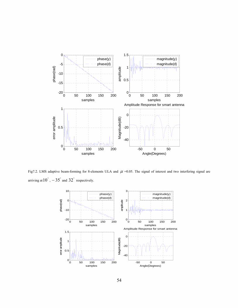
54

0 50 100 150 200-20

-15

-10

-5

0ph

ase(

rad)

samples

phase(y)phase(d)

0 50 100 150 2000

0.5

1

1.5

ampl

itude

samples

magnitude(y)magnitude(d)

0 50 100 150 2000

0.5

1

erro

r am

plitu

de

samples-50 0 50

-40

-20

0

Amplitude Response for smart antenna

Mag

nitu

de(d

B)

Angle(Degrees)

Fig7.2. LMS adaptive beam-forming for 8-elements ULA and μ =0.05. The signal of interest and two interfering signal are

arriving at , and respectively. °10 °− 35 °32

0 50 100 150 200-20

-10

0

10

phas

e(ra

d)

samples

phase(y)phase(d)

0 50 100 150 2000

1

2

3

ampl

itude

samples

magnitude(y)magnitude(d)

0 50 100 150 2000

0.5

1

1.5

erro

r am

plitu

de

samples-50 0 50

-40

-20

0

Amplitude Response for smart antenna

Mag

nitu

de(d

B)

Angle(Degrees)

55

Fig7.3. CMA adaptive beam-forming for 8-elements ULA and μ =0.05. . The signal of interest and two interfering signal are

arriving at , and respectively. °10 °− 35 °32

0 100 200 300 400-40

-20

0

20ph

ase(

rad)

samples

phase(y)phase(d)

0 100 200 300 4000

0.5

1

1.5

ampl

itude

samples

magnitude(y)magnitude(d)

0 100 200 300 4000

0.5

1

ampl

itude

samples-50 0 50

-40

-20

0

Amplitude Response for given Antenne Array

Mag

nitu

de(d

B)

Angle(Degrees)

Fig.7.4. LS- CMA adaptive beam-forming for 8-elements ULA and μ =0.05. . The signal of interest and two interfering signal

are arriving at , and respectively °10 °− 35 °32 The constant modulus algorithm converges slower then least square algorithm .During the

effort to simulate constant modulus algorithm it was clear that the algorithm is less stable than

the least mean square algorithm .The constant modulus algorithm seems to be more sensitive to

gradient constant μ .

The simulation results support the stability and convergence results presented in fig.7.3,

fig.7.4, and demonstrate the superior adaptivity of the least-squares CMA over the steepest-

descent CMA. One severe disadvantage of the CMA is slow convergence time .The slow

converges limits the usefulness of the algorithm in the dynamic environment where the signal

must be captured quickly. This also limits the usefulness of CMA when channel conditions are

rapidly changing. The CMA is based upon the method of steepest descent by taking the gradient

of the cost function. A faster algorithm was developed using the method of non-linear least

square.

56

0 50 100 150 200-20

-15

-10

-5

0

phas

e(ra

d)

samples

phase(y)phase(d)

0 50 100 150 2000

0.5

1

1.5

ampl

itude

samples

magnitude(y)magnitude(d)

0 50 100 150 2000

0.5

1

erro

r am

plitu

de

samples-50 0 50

-40

-20

0

Amplitude Response for smart antenna

Mag

nitu

de(d

B)

Angle(Degrees)

Fig7.5. RLS adaptive beam-forming for 8-elements ULA, 1=λ and 004.0=δ . The signal of interest and two interfering

signal are arriving at , and respectively. °10 °− 35 °32 An important feature of the recursive least square algorithm is that its rate convergence is

typically an order of magnitude faster then that of the simple least square algorithm ,due to fact

that recursive least square algorithm whiten the input data by using the inverse correlation matrix

of the data, assumed to be zero mean . This improvement, however, achieved at the expense of

an increase in computational complexity of the recursive least square algorithm. We verified

with simulation result that the smart antenna minimizes interference noise, and RLS algorithm is

better than CMA, LS-CMA and LMS algorithm.

57

CHAPTER 8

CONCLUSION AND SCOPE OF FURURE WORK

8.1 Conclusion

58

The principle reason for the growing interest in smart antenna systems is the capacity

increase and low power consumption. In densely populated areas, mobile systems are normally

interference-limited, meaning that the interference from other users is the main source of noise in

the system. This means that the signal-to-interference ratio (SIR) is much larger than the signal-

to-noise ratio (SNR). In general, smart antennas will increase the SIR by simultaneously

increasing the useful received signal level and lowering the interference level.

Just by looking at the equations that describe the updating procedures, it is clear that the

RLS algorithm is more complicated than the LMS algorithm. The RLS algorithm has a

computation complexity in the order of square of M, where M is the number of taps or in this

case, the number of elements. For the LMS algorithm, the complexity is in the order of M.

However, the RLS algorithm has much better performance than LMS algorithm. Its rate of

convergence is consistent and is independent of the eigen values of the received signals. It only

takes approximately 2M + 1 iterations to get to the steady state. Moreover, the steady state error

is smaller in magnitude than the one obtained by the LMS algorithm.

CMA algorithm has slower convergence then LMS algorithm. The constant modulus

algorithm is unsupervised algorithm. It optimizes weight of elements in the array without

reference signal. The reference signal is typically a training sequence used to train the adaptive

array or a desired signal based upon priory knowledge of nature of the arriving signal. The LS-

CMA is also an unsupervised algorithm, but its performance is better then CMA algorithm. The

chief advantage of the LS-CMA is that it can converge up to 100 times faster then the

conventional CMA algorithm.

Wireless operators face a sizeable technology challenge as they pursue growth through data

and multimedia services. We have outlined how smart antenna system will contribute to meeting

that challenge, along with continued spectrum efforts and new scale economies in the wireless

supply base. We can expect, smart antenna system will play a key role in wireless

communication.

8.2 Scope of future work

59

The LS-CMA, also known as static LS-CMA, computed the weights simply based upon a

fixed block of sampled data. In order to maintain up-to-date adaptation in dynamic signal

environment, it is better to update the data block for each iteration Thus a dynamic LS-CMA

algorithm [15] is more appropriate. The dynamic LS-CMA is a modification of the previous

static version.

The neural network approach [17] is used to the problem of finding the weights of one- (1-

D) and two-dimensional (2-D) adaptive arrays. In modern cellular satellite mobile

communications systems and in global positioning systems (GPS’s), both desired and interfering

signals change their directions continuously. Therefore, a fast tracking system is needed to

constantly track the users and then adapt the radiation pattern of the antenna to direct multiple

narrow beams to desired users and nulls interfering sources. In the approach suggested, the

computation of the optimum weights is accomplished using three-layer radial basis function

neural networks (RBFNN). The results obtained from this network are in excellent agreement

with the Wiener solution.

References

60

[1] Rappaport T. S., “Wireless Communications: Principles & Practice” Upper Saddle River,

NJ, Prentice Hall PTR, 1999.

[2] Dimitris G. Manolakis , Vinay K.Ingle,Stephen M. Kogon , “Statistical and adaptive signal

processing”, Mc Graw Hill Publication, 2005.

[3] Lal C. Godara, “Application of antenna arrays to mobile communications, part П: beam-

forming and direction-of-arrival considerations”, Proceeding of the IEEE, Vol. 85, No. 8, pp.

1195-1234, August 1997.

[4] Bruno Suard, Guanghan Xu, Hui Liu, and Thomas Kailath, “Uplink Channel Capacity of Space-

Division-Multiple-Access Schemes” IEEE Transaction on Information Theory, Vol. 44. No. 4,

(July 1998): p. 1468-1476.

[5] Salvatore Bellofiore, Consfan fine A. Balanis, Jeffrey Foufz, and Andreas S. Spanias,

“Smart-Antenna Systems for Mobile Communication Networks Part I: Overview and Antenna

Design” IEEE Antenna’s and Propagation Magazine, Vol. 44, No. 3, June 2002.

[6] Carl B. Dietrich, Jr., Warren L. Stutzman, Byung-Ki Kim, and Kai Dietze, “Smart Antennas

in Wireless Communications: Base-Station Diversity and Handset Beam forming” lEEE

Antennas and Propagation Magazine, Vol. 42, No. 5, October 2000.

[7] Jack H. Winters, “Optimum Combining in Digital Mobile Radio with Co-channel Interference”,

IEEE Journal on Selected Areas In Comm., Vol. SAC-2, No. 4, July 1984.

[8] Michael Chryssomallis, “Smart Antennas” lEEE Antennas and Propagation Magazine, Vol.

42, No. 3, June 2000.

[9] Eleftheria Siachalou, EIias Vafiadis, Sotirios S. Goudos, Theodoros Samaras, Christos S.

Koukourlis, and Stavros Panas, “On The Design of Switched-Beam Wideband Base Stations”

IEEE Antennas and Propagation Magazine, Vol. 46, No. 1, February 2004.

[10] Symon Haykin, “Adaptive filter theory”, Forth edition, Pearson education asia, Second

Indian reprint,2002.

[11] Bernard widrow, Semuel D. Stearns, “Adaptive signal processing”, Pearson education asia,

Second Indian reprint,2002.

[12] Angeliki Alexiou and Martin Haardt, “Smart antenna technologies for future wireless

systems: Trends and Challenges”, IEEE Comm. Magazine, vol. 42 ,no.9 ,pp. 90-97, September

2004.

61

[13] Angela Doufexi, Simon Armour, Andrew Nix, Peter Karlsson, and Dave Bull “Range

andThroughput Enhancement of Wireless Local Area Networks Using Smart Sectorised

Antennas” IEEE transaction on wireless communications,vol.3, no. 5, September 2005.

[14] Salvatore Bellofiore, Jeffrey Foutz, Constantine A. Balanis, and Andreas S. Spanias,

“Smart-Antenna System for Mobile Communication Networks Part 2: Beamforming and

Network Throughput” IEEE Antenna's and Propagation Magazine, Vol. 44, NO. 4, August 2002.

[15] Frank Gross, “Smart Antenna For Wireless Communication” Mcgraw-hill, September 14,

2005.

[16] Agee, B, “The Least-Square CMA: A New Technique for Rapid Correction of Constant

Modulus Signal” IEEE International Conference on ICASSP’86, Vol. 11, pp. 953-956, April

1986.

[17] A. H. El Zooghby, C. G. Christodoulou, and M. Georgiopoulos, “Neural Network-Based

Adaptive Beamforming for One- and Two-Dimensional Antenna Arrays” IEEE Transaction on

Antennas and Propagation, Vol. 46, No. 12, DECEMBER 1998

62