IN DEGREE PROJECT ELECTRICAL ENGINEERING,SECOND CYCLE, 30 CREDITS

, STOCKHOLM SWEDEN 2016

A STUDY OF A MULTI BAND ANTENNA’S PERFORMANCE FOR DIFFERENT FREQUENCIES AND RADIO ACCESS TECHNOLOGIES

KULDEEP PAREEK

KTH ROYAL INSTITUTE OF TECHNOLOGYSCHOOL OF INFORMATION AND COMMUNICATION TECHNOLOGY

Kuldeep Pareek

Master of Science Thesis performed at the Radio Systems Lab,Communication Systems Department School of ICT, KTH

September 2016

Internal Advisor : Mats NilsonExternal Advisor : Tord SjölundExaminer : Ben Slimane

�i

A STUDY OF A MULTI BAND ANTENNA’S PERFORMANCE FOR DIFFERENT FREQUENCIES AND RADIO ACCESS TECHNOLOGIES

�ii

Abstract:

There has been and will be a constant development in the field of communication

systems and telecommunication in the form of network designs, access technologies, and equipment. Today, most of the mobile users are in indoors environments such as

buildings, metros, arenas etc. These users are becoming impossible to serve from outdoor base station antenna because of energy-effective building techniques, which

have RF shielding properties. A solution to this is to move antenna closer to the users in the indoor environment. There is a need to find a cost effective and economical

and environmental solution to this switch. Generally, a separate deployment for RAKEL, 2G, 3G and LTE each is done for indoor coverage. With the use of a Multi

band antenna, all the above radio access technologies can be deployed while sharing hardware.

This thesis investigates one such multi band antenna’s performance parameters for

frequencies ranging from 380 MHz to 2700 MHz and provides a case study which analyses multiple deployed network locations and design where the antenna is

deployed while serving RAKEL, 2G, 3G and LTE.

�iii

Sammanfattning

Telekommunikationer har varit under konstant utveckling ända sedan vi började

använda mobil kommunikation. Ständig utveckling av system design, olika teknologier och utrustningar. Idag sker den mobila kommunikationen i

inomhusmiljöer, kontor, gallerior, hotell, tunnelbanor, sportarenor etc.  Trafiken från just dessa anläggningar är i storleksordning 70 – 80 % av all trafik vilket gör

det omöjligt att serva dessa användare från basstationer utomhus och med dagens energikrav på nya byggnader stänger effektivt ut alla radiosignaler från

utomhus siter. En lösning är att flytta antennen närmare användaren vilket också innebär att hitta nya kosteffektiva lösningar för just denna typ av miljöer. Idag så

designar man  inomhusanläggningar för samtliga operatörer, 2G, 3G, LTE samt RAKEL. Användandet av en multiband-antenn  kan man dela den mobila

infrastrukturen med olika teknologier vilket innebär minskade kostnader.  

Examensarbetet uppgift var att undersöka egenskaperna hos denna multiband antenn för frekvenserna 380 – 400 MHz, 698 – 2700 MHz och också fältstudier

från redan installerade för RAKEL, 2G, 3G och LTE.

�iv

Acknowledgment:

I would like to thank my supervisors Mats Nilson (KTH) and Tord Sjölund (MIC Nordic) for providing me continuous support throughout the thesis, without their

support it would be impossible to finish this thesis on time. Secondly, I would like to thank my examiner Ben Slimane for providing me his support in the existence

of such unrealistic deadlines. I would also like to especially thank Leif Eriksson and Bikash Shakya at MIC Nordic who taught me so much about antenna’s and

indoor network components. I would extent my gratitude to the whole team at MIC Nordic for providing me a great work environment. Finally, I would like to thank my

parents for pushing me to get a higher education and inspiring me, without their support I would not have been in the academic field in the first place

�v

Table of Content

List of Figures viiiList of tables ixAcronyms and Abbreviation xChapter 1: Introduction 11.1 Background 11.2 Previous work 31.3 Research Problem 31.4 Method 41.5 Ethics 41.6 Limitations 5Chapter 2: Theory 62.1 Link Budget 62.2 Propagation Models 8 2.2.1 Free Space Path Loss 8 2.2.2 The Modified Indoor Model 10 2.2.3 The Path loss slope Indoor Model 10 2.2.4 Empirical Models 11 2.2.5 Fast Ray Tracing Model 132.3 Antenna types 14Chapter 3 Technology background 163.1 System Technology 16 3.1.1 RAKEL/ Tetra 16 3.1.2 GSM 16 3.1.3 UMTS 17 3.1.4 LTE 17 3.1.5 WLAN 2.4 GHz 183.2 Indoor Systems 20 3.2.1 Traditional Indoor Systems 20 3.2.2 Integrated Indoor Systems 20 3.2.3. Radiating cables (Leaky Feeder) 20 3.2.4 Distributed antenna system 21

�vi

Table of Content

Chapter 4 Methodology 254.1 Antenna analysis Measurements and Methodology: 254.2 System Design: 264.2.1 Active Network design 26 4.2.2 Measurement tools 29 4.2.3 Measurement locations 30 4.2.4 Link Budget calculations 33Chapter 5 Result and Discussion: 345.1 Antenna Analysis: 345.2 Coverage Analysis: 40Chapter 6 Conclusion 49Chapter 7 Future work 50References: 51

�vii

List of Figures

Figure 1.1 :MIC 360 antenna………………………….…………………..……2Figure 2.1 :Link Budget………………………….………………………………6

Fig 2.2.1 : :Free space path loss………………………….……………………9Fig 3.1.4 :Evolution of LTE from GSM and UMTS ……………………..….18

Figure 4.2.1 :Active DAS network design used………………………….……..28Figure 4.2.3.1:Floor Plan Building 1 & 2 ………………………….………………30

Figure 4.2.3.2: Antenna Placement Building 1 & 2 ……………………………..31Figure 4.2.3.3 :Floor Plan Building 3………………………….………….………..31

Figure 4.2.3.4 :Antenna Placement Building 3………………………….………..32Figure 5.1.1 :S11 MIC 360 antenna………………………….…..…….………..36

Figure 5.1.2 :Smith Chart 380-490 MHz MIC 360 antenna………….………..37Figure 5.1.3 :Smith Chart 800-900 MHz MIC 360 antenna………….………..37

Figure 5.1.4 :Smith Chart 1800-1900 MHz MIC 360 antenna……….………..38Figure 5.1.5 :Smith Chart 2600-2700 MHz MIC 360 antenna……….………..38

Figure 5.2.1 :Antenna placement building 1 and 2……………………………..40Figure 5.2.2 :Antenna Placement building 3……………………………….……41

Figure 5.2.3 :Site Master Screen Shot………………………………………..…43Figure 5.2.4 :Rakel Terminal screenshot………………………………..………45

Figure 5.2.5 :Tems screenshot………………………………………….……….46Figure 5.2.5 :Spectrum analyser screen shots ………………………..………47

�viii

List of tables

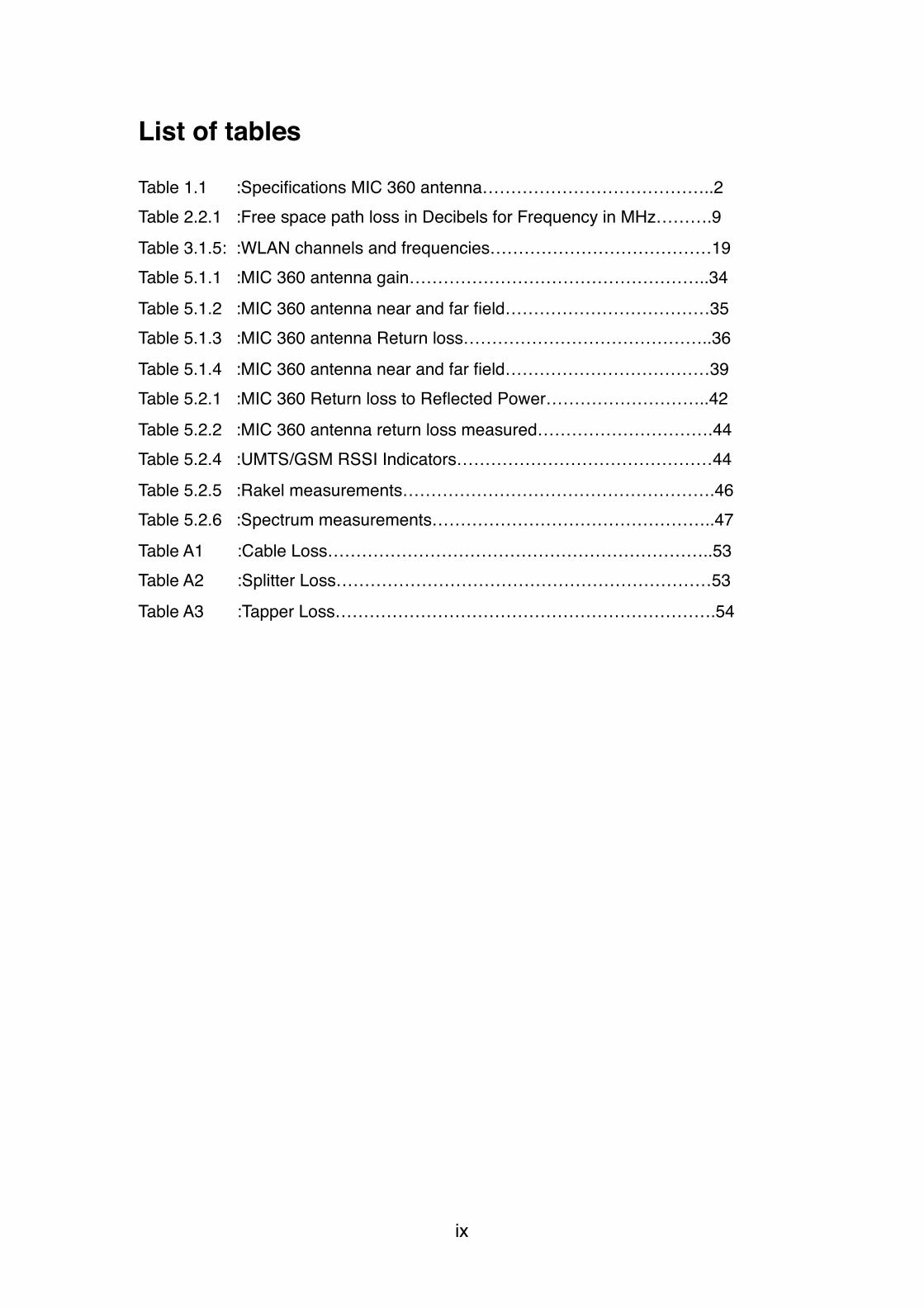
Table 1.1 :Specifications MIC 360 antenna…………………………………..2Table 2.2.1 :Free space path loss in Decibels for Frequency in MHz……….9

Table 3.1.5: :WLAN channels and frequencies…………………………………19Table 5.1.1 :MIC 360 antenna gain……………………………………………..34

Table 5.1.2 :MIC 360 antenna near and far field………………………………35Table 5.1.3 :MIC 360 antenna Return loss……………………………………..36

Table 5.1.4 :MIC 360 antenna near and far field………………………………39Table 5.2.1 :MIC 360 Return loss to Reflected Power………………………..42

Table 5.2.2 :MIC 360 antenna return loss measured………………………….44Table 5.2.4 :UMTS/GSM RSSI Indicators………………………………………44

Table 5.2.5 :Rakel measurements……………………………………………….46Table 5.2.6 :Spectrum measurements…………………………………………..47

Table A1 :Cable Loss…………………………………………………………..53Table A2 :Splitter Loss…………………………………………………………53

Table A3 :Tapper Loss………………………………………………………….54

�ix

Acronyms and Abbreviation

DAS Distribute antenna systemEM Electro MagneticPIM Passive IntermodulationEIRP Equivalent isotropically radiated powerERP Effective Radiated powerFSPL Free Space Path Loss PLS Path Loss ConstantRU Remote UnitMU Master UnitWLAN Wireless Local Area NetworkTETRA Terrestrial Trunked RadioUMTS Universal Mobile Telecommunication SystemWCDMA Wide band Code Division Multiple AccessDS-CDMA Direct-Sequence Code Division Multiple AccessGSM Global System for Mobile CommunicationFDD Frequency Division DuplexTDD Time Division DuplexFDMA Frequency Division Multiple AccessTDMA Time Division Multiple AccessDSSS Direct Sequence Spread SpectrumFHSS Frequency Hoping Spread SpectrumMIMO Multiple Input Multiple OutputRSSI Received Signal Strength IndicationRSCP Received Signal Code PowerRSRP Received Signal Reference Power

3GPP 3rd Generation Partnership Project

�x

Chapter 1: Introduction

1.1 Background

In 1830 the first telecommunication system was introduced and within less than two centuries it has developed to a point where it has integrated deep into our lives. We are using telecommunication in the form of various access technologies such as TETRA, 2G, 3G, 4G, IEEE 802.11 WLAN and soon 5G will be introduced. Each new radio access technology offers more features in the form of bandwidth, capacity, and coverage.

At this point, we are able to provide coverage to even remote outdoors and indoors but with the introduction of energy efficient building techniques and materials such as energy efficient glasses, walls, and doors it is becoming impractical to use the same outdoor network to provide coverage within the indoor buildings and environments.

“Some 70-80% of Mobile Traffic is Inside Buildings” [1], Such buildings are airports, offices, industrial plants tunnels, homes, arenas, malls, schools, and universities etc. Large traffic demands are impossible to fulfil with the outdoor base station antennas thus a solution to this is to bring antenna’s capacity closer to the users, which is now already being implemented at various locations in the form of indoor distributed antenna systems for TETRA, 2G, 3G, 4G, IEEE 802.11 WLAN.

Currently, separate distributed antenna systems for each of the above access technologies and different operators are generally deployed, which is an expensive and non-efficient use of the distributed antenna system and also consuming more energy as separate equipment for each radio access is used. A solution to this is provided in the form of a master unit which takes in multiple different transmission signals at different frequency bands and combines them with the use of multiple combiners and repeaters. This signal is combined to generate a wide band signal, which the master unit transmits to a Multi band antenna distribution system and thus with the use of a distributed antenna system the coverage for TETRA, 2G, 3G, 4G and IEEE 802.11 WLAN can be deployed.

MIC Nordic is a system integrator which provides solutions from preliminary assessment to the final deployment of the network has developed a multi band

�1

antenna for frequencies from 380 MHz to 2700 MHz that supports TETRA, 2G, 4G , IEEE 802.11 WLAN and possibly also 5G networks. The deployment of this antenna in a distributed antenna system not only reduces the overall all cost of deployment of this radio access technologies but also makes the network future proof for the introduction of 5G radio access technology to be introduced in the supported frequency bands in the nearby future.

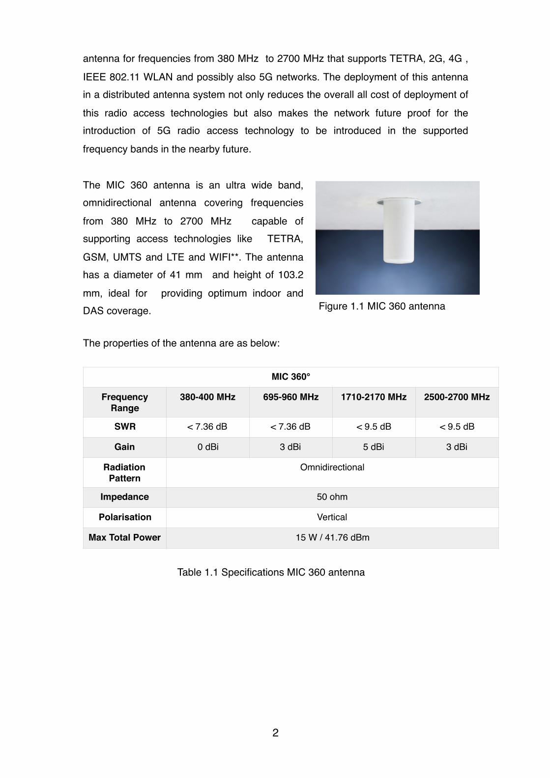
The MIC 360 antenna is an ultra wide band, omnidirectional antenna covering frequencies from 380 MHz to 2700 MHz capable of supporting access technologies like TETRA, GSM, UMTS and LTE and WIFI**. The antenna has a diameter of 41 mm and height of 103.2 mm, ideal for providing optimum indoor and DAS coverage.

The properties of the antenna are as below:

MIC 360°

Frequency Range

380-400 MHz 695-960 MHz 1710-2170 MHz 2500-2700 MHz

SWR < 7.36 dB < 7.36 dB < 9.5 dB < 9.5 dB

Gain 0 dBi 3 dBi 5 dBi 3 dBi

Radiation Pattern

Omnidirectional

Impedance 50 ohm

Polarisation Vertical

Max Total Power 15 W / 41.76 dBm

�2

Figure 1.1 MIC 360 antenna

Table 1.1 Specifications MIC 360 antenna

1.2 Previous work

There has been some previous works on the indoor broadband antenna’s capable of transmitting signals in GSM/UMTS/LTE for 1.5 GHz to 2.8 GHz and for Wifi at 4.7 GHz to 8.5 GHz [13] [14] but most of such antennas have return loss in the range of 10 dB in the compatible frequency ranges.

The paper titled “ A Dual-Broadband MIMO Antenna System for GSM/UMTS/LTE and WLAN Handsets” [13] by Xiang Zhou explains the broadband antenna in much detail and this thesis extends the work done in the paper.

Another thesis at KTH titled “A study on multi-band radio distribution system” [14] describes in much detail the feasibility and cost of using such antenna in a distributed antenna system, this thesis is a continuation of that work.’

Some of the work has also been inspired greatly by the previous work in the publication titled “Factors influencing outdoor to indoor radio wave propagation” [15] by S. Stavrou which describes how the traditional variables and factors change when serving a user with an outdoor macro cell vs and indoor minor cell.

1.3 Research Problem

The introduction of energy effective materials and their shielding properties has made it infeasible to serve the indoor user with the outdoor macrocell network. Users have to open their windows and doors in order to get a signal in their devices as the attenuation of this energy effective materials is quite high, this is also addressed in a previous thesis [14]. The opening of the windows also adds to increased energy consumption because of the heat loss factor [16].

Multiple solutions for the indoor networks are sometimes deployed separately for different radio access. A wide band distributed antenna system indoors along with a master unit which combines all the different radio access technologies as TETRA, 2G, 3G, 4G, IEEE 802.11 WLAN can be an effective solution for addressing the indoor signal strength and also the deployment costs.

The focus of this thesis will be on solving the following:

�3

• There are multiple variables which are used for antenna analysis which include return loss and impedance matching which should be tested for this antenna for a wide range of frequencies to predict the selected antenna’s feasibility.

• A detailed analysis is required of the broadband antenna used in indoor network deployment for a multitude of radio access technologies as TETRA, 2G, 3G, 4G, IEEE 802.11 WLAN.

• Also, the properties of this antenna in the frequencies outside its range should also be checked to predict the feasibility of the antenna in such frequencies.

1.4 Method

To provide answers to the research question in this thesis the process will be divided into the following steps in the respective order:

• Literature studies to understand the variables for antenna analysis and indoor network planning.

• Analysis of the antenna.

• Choose optimal test location for the analysis.• Test location network study.

• Take measurements in the test location for coverage analysis.• Measurement and result from analysis and documentation.

1.5 Ethics

Access to communication technologies in some constitutions (Estonia) has been described as basic human rights. And a part of the population should not be denied an access to mobile networks because they are indoors in a tunnel or a newly constructed building. This thesis plays it own small but significant role in laying the foundation towards moving the communication indoors. Also as described previously in a thesis[ 16] that just the opening of windows in a building increases the energy-consumption by a significant amount. Moving the network indoors might to some level

�4

will prevent users from opening windows and this will lead to a high energy saving when combined for multiple locations

1.6 Limitations

There can be certain limitations in providing the coverage analysis for this thesis in the form of lack of locations where all TETRA, GSM, 3G and LTE are deployed. Also sometimes the operators are not comfortable in making the network design of their networks public, thus limiting some content of this thesis. For coverage analysis the location chosen is designed for TETRA, GSM, 3G and LTE, but because all the access technologies were not deployed by the operators in the time frame of thesis, we will skip coverage analysis for GSM and LTE.

�5

Chapter 2: Theory

2.1 Link Budget

The Link budget is the basic block of indoor modeling, it basically describes how much power went out with respect to how much power went in a system.It describes how much power was attenuated in every block of the system.

Elements of a link budget:

Transmitter output power: Transmitter output is the power emitted by the transmitter.

Transmitter antenna gain: Gain can be defined as how much power went out relative to how much power went in. The relative increase in power transmitted by the antenna with respect to the power received by the transmitter.

Receiver antenna gain: The relative increase in power transmitted to the receiver by the antenna with respect to the power received by the transmitted antenna

Cable Loss: Intensity reduction of a signal transmitting through a cable

�6

Figure 2.1 Link Budget

Propagation path loss: Intensity reduction of a signal transmitting through free space/walls etc. Path loss is frequency and distance dependent.

Effective Isotropic Radiated Power (EIRP):EIRP is the effective amount of power that is radiated by a transmitting antenna.EIRP can be denoted as EIRP = Transmitter power - cable loss + antenna gain

the Link Budget is the gain and loss calculation for a system, a typical calculation looks like

Where,Prx = Received Power Ptx = Transmitted PowerGt = Transmitting antenna gainLtx = loss on the transmitting side (feeder, cable, combiner, external filters etc)Lp = Path lossGrx = Receiving antenna gainLrx = Loss on receiver side(Feeder, cable etc)Lms = miscellaneous loss (Mismatch, fading, Margins etc)

�7

2.2 Propagation Models

To predict the strength of a signal at any location, a path loss model has been used during the design phase. So that the resulting measurements after the deployment can be as close to the desired strength level. A propagation model predicts the characteristics of a radio signal with respect to the environment.A propagation model is basically an algorithm in the form of a mathematical expression. A Propagation model is generally more accurate for lower radio frequencies compared to the higher radio frequencies as the lower frequencies are less affected by the objects around in the environment compared to the higher frequencies (refer to free space path loss table on page 9).

2.2.1 Free Space Path Loss

Free space path loss is calculated using the assumption that there is a line of sight between the receiver and the transmitter without the presence of any object in between.The model can be mathematically described as [3]

or

where Pr is termed as the received power and Pt as power transmitted.D is the free space distance and Ct is the transmitter’s constant

�8

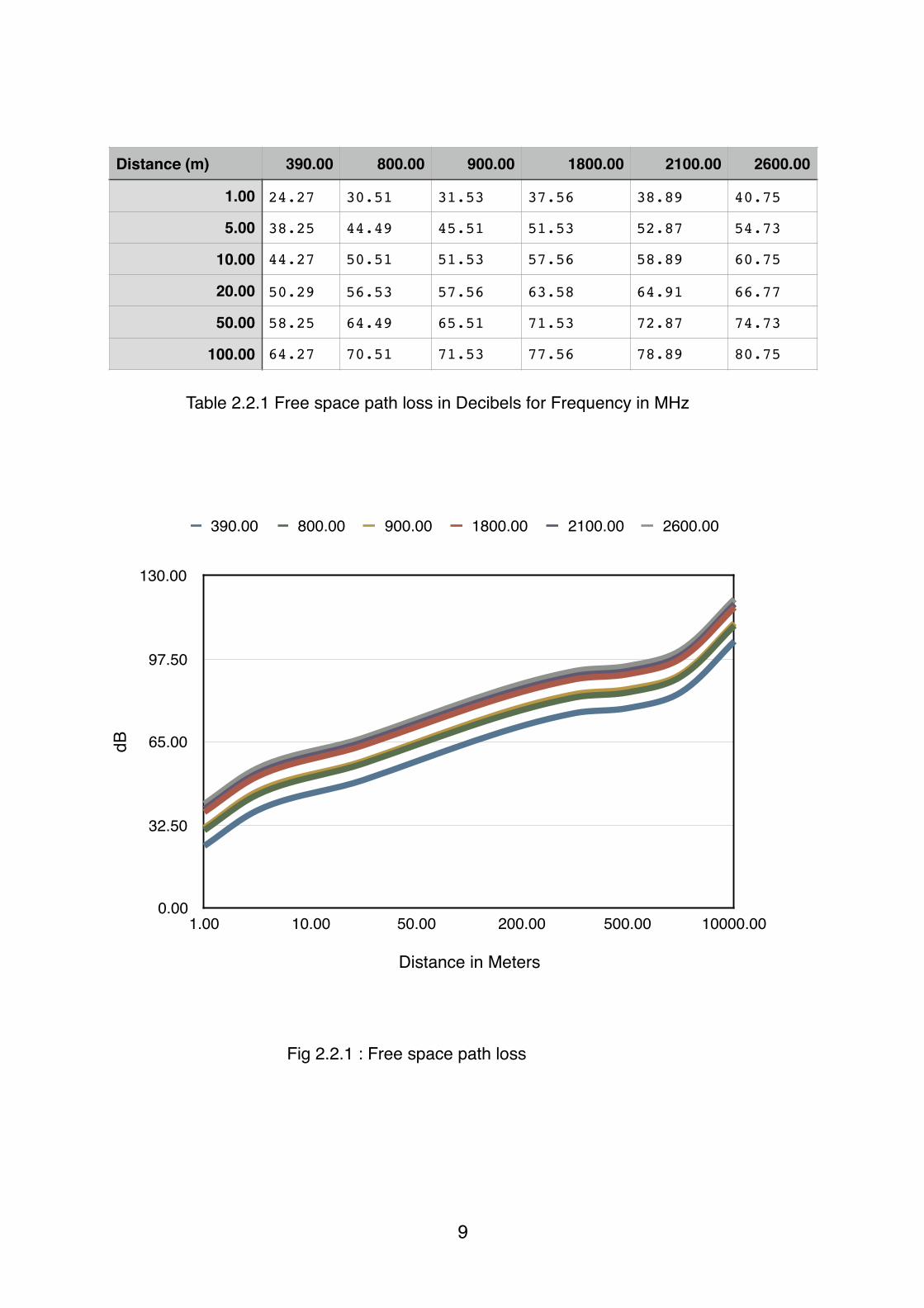
Table 2.2.1 Free space path loss in Decibels for Frequency in MHz

Distance in Meters

Fig 2.2.1 : Free space path loss

�9

Distance (m) 390.00 800.00 900.00 1800.00 2100.00 2600.00

1.00 24.27 30.51 31.53 37.56 38.89 40.75

5.00 38.25 44.49 45.51 51.53 52.87 54.73

10.00 44.27 50.51 51.53 57.56 58.89 60.75

20.00 50.29 56.53 57.56 63.58 64.91 66.77

50.00 58.25 64.49 65.51 71.53 72.87 74.73

100.00 64.27 70.51 71.53 77.56 78.89 80.75

dB

0.00

32.50

65.00

97.50

130.00

1.00 10.00 50.00 200.00 500.00 10000.00

390.00 800.00 900.00 1800.00 2100.00 2600.00

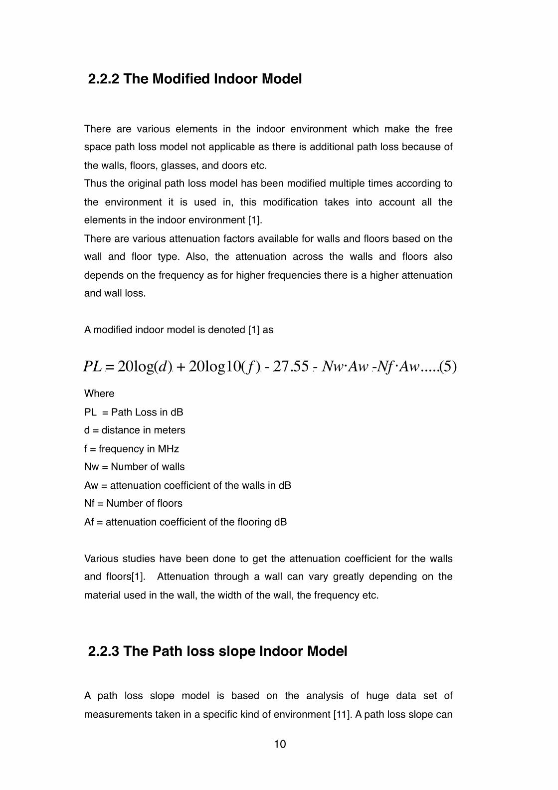
2.2.2 The Modified Indoor Model

There are various elements in the indoor environment which make the free space path loss model not applicable as there is additional path loss because of the walls, floors, glasses, and doors etc.Thus the original path loss model has been modified multiple times according to the environment it is used in, this modification takes into account all the elements in the indoor environment [1]. There are various attenuation factors available for walls and floors based on the wall and floor type. Also, the attenuation across the walls and floors also depends on the frequency as for higher frequencies there is a higher attenuation and wall loss.

A modified indoor model is denoted [1] as

WherePL = Path Loss in dBd = distance in metersf = frequency in MHzNw = Number of wallsAw = attenuation coefficient of the walls in dBNf = Number of floors Af = attenuation coefficient of the flooring dB

Various studies have been done to get the attenuation coefficient for the walls and floors[1]. Attenuation through a wall can vary greatly depending on the material used in the wall, the width of the wall, the frequency etc.

2.2.3 The Path loss slope Indoor Model

A path loss slope model is based on the analysis of huge data set of measurements taken in a specific kind of environment [11]. A path loss slope can

�10

be derived by taking the repetitive measurements of the same kind of environment . The process involves taking RSSI measurements from multiple distances from the antenna and a huge data is collected for analysis.Thus different environments will have different path loss slope characteristics. To get more accurate results it is necessary to use the specific PL constant[11]

The calculation [11] can be denoted as

Where,

PL = Path LossFSPL = Free Space Path LossPLS = path loss constant

PLS here is environment specific.

Example[11]:

PLS open environnement for 900 MHz 30.1PLS dense environment for 900 MHz 39.4

2.2.4 Empirical Models

In some cases, the above path loss models are not applicable such as in uneven terrains or in cities with high buildings, where because of reflection and lack of information about some variables makes it impossible to predict the path loss for a radio frequency signal. In such cases, empirical path loss models can be used which is based on extensive measurements.There are various empirical path loss models based on the environment for which oath loss has to be predicted.

�11

• Hata Model

Hata model is based on extensive field test measurements, It has many variations for different environments such as semi-urban, rural, open terrain, urban with high buildings, but Hata model has also various limitations like it is only suitable for frequencies from 150 MHz- 1500 MHz thus will be suitable for GSM (900 MHz) but not for UMTS (2100 MHz), distance from base station from 1km - 20 km thus will not be suitable for indoor environments, height of antenna from 30m-200m and the height of mobile antenna ranging from 1m-10m [4]

• Cost 231

Cost 231 is an extended version of Hata model and is suitable for up to 2GHz thus making it also a suitable model to use for 3G path loss predictions[20].It is also compatible with lower antenna heights, thus is also suitable for indoor propagation modelling.

• TGn Model This is a path loss model used for IEEE 802.11 TGn channel.

It can be described as [5] :

Path is equal to free space path loss for distance < breakpoint distance

IEEE describes that tGn model can be used with free space path loss model for distances less that the breakpoint and one slope model for distances high that the breakpoint. Where the breakpoint distance is described as 5m and 10m for small and large environments respectively.

An empirical path loss model is only significant if used for the matching environment, otherwise, such models have a poor accuracy for the environment which it does not relate to.

�12

2.2.5 Fast Ray Tracing Model

When there is a need for more accurate predictions for propagation for indoor environments , where real tracing come into the scenario.There are two methods to do ray tracing measurements [6]

• Image method

Image method is more useful for environments which are more simple and have less number of overall reflections

• Brute force method:

Brute force method is a CPU intensive and time-consuming process which involves detailed antenna characteristics, the angle of reflections etc.

In this method multiple rays leave the transmitter in all directions which might or might not reach the receiver, it is necessary to consider all the angles for the ray at the transmission side and well as the receiving side. It is of importance that all the rays leaving have the same characteristics at 1 m distance from the transmitter [6] so that accurate measurements can be taken at every angle.

The Transmitter in brute force method is designed as a spherical arrangement of multiple simulated tubes so that all the angles around it can be covered. Same kind of equipment is placed on the receiver side. Then iteratively signals are transmitted from every angle by the transmitter and received measures the strength of a signal received and in the process providing an extensive propagation model for the environment.

Ray tracing can be considered as the most accurate way of modeling the propagation in an indoor environment. As it is measurement based using transmitters and receivers rather than theoretically predicted.

�13

2.3 Antenna types

An antenna is the end point or beginning of a radio network. The RF radiation in an antenna is facilitated by the electric charge that is accelerating or decelerating on the antenna. An antenna converts a guided EM wave from the generator to a wave launched in free space through a transmission line and a transition region. And an incident wave is converted into guided wave for the receiver.

There are various kinds of antenna designs used based on the required frequency and radiation patterns.

• Electrical small antenna

In electrically small antenna’s the size of the antenna is less that the wavelength of the corresponding frequency it is designed for [7]. This kind of antennas have a very low directivity, resistance, and radiation efficiency but they have a very high input reactance.

These antennas can be used as receiver sensors where they don’t have to transmit signals but wait for the signal for the signal to begin any programmed process for example sensors electronic devices etc.

• Resonant antennas

A resonant antenna designed is generally used for serving a very narrow frequency band [7]. Thus they have a very narrow bandwidth and low gain.

• Broadband antennas

A broadband antenna is designed to be stable across a wide band of frequencies, thus having a stable gain and pattern around all the frequencies it is designed for [7], the antenna used for the purpose of this thesis is a multi resonant antenna.

�14

• Aperture antenna

This antenna has an opening through which waves enter the transition region, the antenna has very high directivity and gain and also can be used across a moderate range of frequencies.[7]

• Isotropic antenna

When the radiation pattern for an antenna is similar in all the directions, such antenna can be defined as an isotropic antenna. This is a theoretical antenna used for reference purpose to describe real antennas.

�15

Chapter 3 Technology background

3.1 System Technology

3.1.1 RAKEL/ Tetra

Tetra is a radio access technology used by emergency services like police, fire brigade etc. In Europe Tetra uses frequencies ranging from 380 to 430 MHz. FD/TDMA is used in Tetra to divide the frequency channels which use 25 KHz spacing and is further divided into 4 sub channels each by time division. The sub channels transmit the information simultaneously over a single carrier channel. Receivers choose the channel with the strongest signal. TETRA has both P2P and broadcast capabilities. Also an underlying network or terminal to terminal connections are also possible. The above redundancies and safety features make TETRA an optimal solution for emergency services [17]. The so-called RAKEL system is used in Sweden by emergency services and is based on TETRA standard

3.1.2 GSM

“With around 5-6 billion subscribers, GSM is the world's most commonly used technology for wireless communication” [1] GSM (Global System for Mobile Communications was concurrently developed in Europe and the USA in the 1980’s. [1]. GSM includes various services such a Voice at 3.1 KHz, SMS (short message service), EDGE, GPRS (General Packet Radio Service) which is an always-on IP based packet data transmission ip to 114 kbps. Initially GSM was designed for 900 MHz range which is now also using 800 MHz, 1800 MHz and 1900 MHz. GSM 900 using two 35 MHz duplex bands for uplink and downlink each separated by a 45 MHz duplex distance where uplink uses 880-915 MHz and downlink uses 925-960 MHz. For GSM 1800 two 75 MHz duplex bands are used for uplink and downlink each along with a 95 MHz guard band where the uplink is from 1710-1785 MHz and downlink is from 1805-1880 MHz. The use of FDD (frequency division duplexing ) and TDD (time division duplexing ) allows GSM to serve multiple number of users. With FDD each frequency band is subdivided into 200 KHz bands each and with TDD each of this 200 KHz band is further divided into 8 time slots.

�16

3.1.3 UMTS

UMTS (Universal Mobile Telecommunication System) is a 3G radio access technology and is step further from GSM providing a higher spectral efficiency and network capacity. It is power limited on downlink and noise limited on uplink [1]

UMTS features WCDMA-TDD and WCDMA FDD: WCDMA-TDD uses the same frequency for uplink as well as downlink in alternative times slots with a guard time in between to minimise interference while WCDMA-FDD uses separate uplink and downlink frequencies separated by 190 MHz. WCDMA is also an effective solution to the frequency selective fading [18]

UMTS uses 1920-1980 MHz for uplink and 2110-2170 MHz for downlink. . Same frequency for neighbouring cells is used in UMTS. Thus an interference from the outside network will affect the indoor network which can be avoided in the case of GSM. A UMTS carrier has an effective bandwidth of 4.75 MHz and is further divided into 3.84 Mchips, where the chips are the raw modulation symbol rate on the carrier [1]

3.1.4 LTE

Long Term Evolution also termed as LTE or 4G is a successor of GSM and UMTS with higher data speeds and increased capacity. It has an ip based network architecture at its core which also supports seamless handovers and multicast and broadcast streams. Today LTE supports frequency bands from existing GSM/WCDMA and also on parts of 700/800/2700 MHz and supports both FDD (Frequency Division Duplexing ) and TDD (Time Division Duplexing) .

LTE supports scalable carrier bandwidth from 1.4 MHz to 20 MHz [2]. The features of LTE include high downlink speeds of up to 300 Mbits / Seconds and an uplink speed of 75Mbits / second and a transfer latency of 5 ms in RAN [2]

The Image below from 3GPP shows the evolution of LTE from GSM and UMTS.

�17

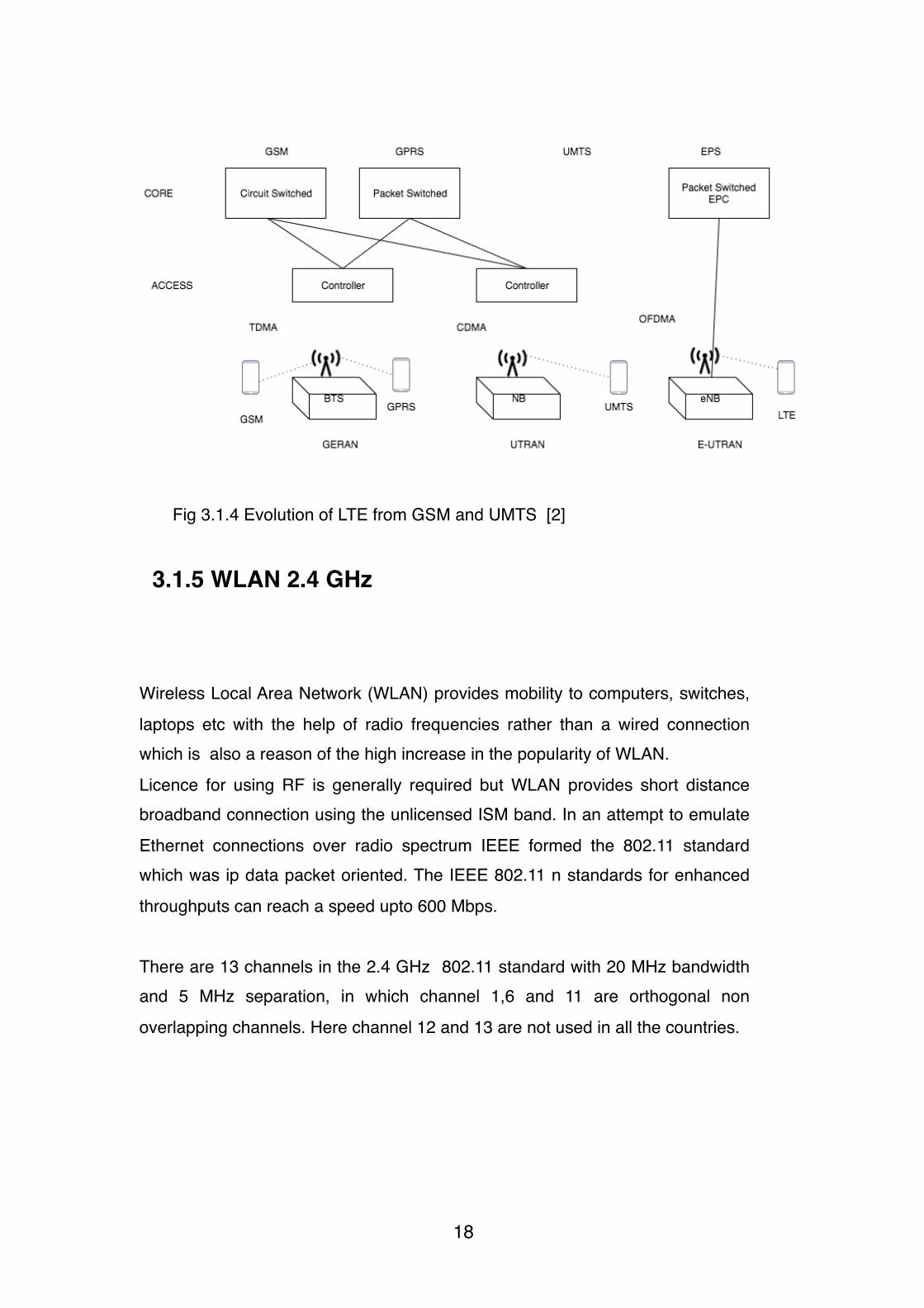
Fig 3.1.4 Evolution of LTE from GSM and UMTS [2]

3.1.5 WLAN 2.4 GHz

Wireless Local Area Network (WLAN) provides mobility to computers, switches, laptops etc with the help of radio frequencies rather than a wired connection which is also a reason of the high increase in the popularity of WLAN.Licence for using RF is generally required but WLAN provides short distance broadband connection using the unlicensed ISM band. In an attempt to emulate Ethernet connections over radio spectrum IEEE formed the 802.11 standard which was ip data packet oriented. The IEEE 802.11 n standards for enhanced throughputs can reach a speed upto 600 Mbps.

There are 13 channels in the 2.4 GHz 802.11 standard with 20 MHz bandwidth and 5 MHz separation, in which channel 1,6 and 11 are orthogonal non overlapping channels. Here channel 12 and 13 are not used in all the countries.

�18

Table 3.1.5: WLAN channels and frequencies

There are two ways of Implementing a WLAN system• Adhoc (Independent Basic Service Set)

• Similar Functionality in all elements • All provide STA (Station) and DS(Distribution Service)

• Access point (Infrastructure Basic Service Set)• Access point concentration all the communication

• Only Access point provides STA and DS service

Channel Center frequency Mhz

1 2412

2 2417

3 2422

4 2427

5 2432

6 2437

7 2442

8 2447

9 2452

10 2457

11 2462

12 2467

13 2472

�19

3.2 Indoor Systems

Multiple radio access technologies need to have signal strength inside the buildings such as RAKEL, 2G, 3G, 4G and WLAN IEEE 802.11. There are multiple ways to fulfil the signal requirements inside, such as coverage from the outdoor networks , small indoor cells or using leaky cables and Distributed Antenna System (DAS) which is also the most commonly used.The most relevant solutions are described below.

3.2.1 Traditional Indoor Systems

The traditional indoor service includes the coverage from an outdoor macro cell . Because of the high attenuation of the building materials etc it is quite difficult to reach the signals levels required. This method generally requires an outdoor macro cells network dense and powerful enough to penetrate through the building material. It mainly relies on reflection for the coverage [1].

3.2.2 Integrated Indoor Systems

Multitude of frequencies are required for indoor access. Services such as TETRA, GPS, wifi etc are generally installed separately. It is hard to convince a customer to install a purely active solution which is a bit more expensive. In this thesis we investigate the option of installing all such radio access technologies using a single solution. This could be especially difficult because of different attenuation of different frequencies for cables and also for the free space, because of which link budget calculation for one radio access does not apply for another.

3.2.3. Radiating cables (Leaky Feeder)

Because of the harsh environments in tunnels for which an antenna system is although a cheap option often not at all suitable. Some of reasons include wind load, vibrations, RF blocking etc. A much more uniform and easy way to plan network for such environments is using radiating cables. It is an optimal solution for tunnel radio networks.

�20

A radiating cable which is also known as leaky feeder is a kind of coaxial cable with components such as• a dielectric

• Inner conductor• Outer shield with slots

The cable can be thought of as many small antennas of one big antenna and can be optimised for coupling losses, insertion loss, frequency etc. t[1]

A few characteristics of the cable to be considered designing a system can be [1]• Longitudinal loss:

• Frequency range • Coupling loss

• System Loss• DC Resistance

3.2.4 Distributed antenna system

There are multiple Distributed antenna network designs available for indoor network coverage design such as

• Active distributed antenna system, • Passive distributed antenna system Both of the active and passive designs have their advantages and disadvantages. A design is chosen on a case to case scenario based on the environment, building, coverage requirements, installation and maintenance costs etc.A key point to consider in the design is to choose for the specific scenario a design with the highest downlink power and the lowest uplink noise.

The two most used design strategies are:

Passive Distributed antenna system:

Passive DAS is the most popular indoor coverage design[1], which can be easily designed by making link budget calculations to the antenna. It can be used in a location where the environmental conditions can easily degrade the active components and is more suitable for small buildings where the antenna is closer to the source thus minimising the loss, it was the most popular choice for the GSM but

�21

is not very suitable for 3G and 4G because of high losses at high frequencies and also because of high return loss. A disadvantage of passive distributed antenna system is the lack of voltage standing wave radio alarm (VSWR), which makes remote monitoring infeasible.

Passive components

Here we describe the most commonly used passive equipment and their function used when designing and indoor coverage system. The use of the equipment also depends on the specification of the building for example when designing a passive system for a hospital some specific material for cables etc might only be permitted.

Coax Cables

Coax or coaxial cables are abundantly used when designing an indoor coverage system. Different cable have a different level of losses, and it is very important to choose the right cable type for the link budget calculations as the losses can vary over cable type and the frequency for which it is used (see Appendix A).

SplitterSplitter is used to divide the signal from one source to multiple, such as signal coming from one coaxial cable to multiple antennas. Splitter also has an insertion loss (see Appendix A).

Tapper

Tappers can be defined as uneven splitters where one port has more power loss compared to another.In the table about tapper in appendix is the tapper loss specification in dB, “loss” is the loss in dB for pass through ports and through port is the loss for ports where the power has to be tapped (see Appendix A).

Attenuators

Attenuators are used to attenuate the signal mostly to keep the power at the antennas equal or to keep the amplifiers for malfunctioning .

�22

Active Distributed antenna system:

An active distributed antenna system uses active components such as Remote units, Master Units, Repeaters, Thin cables and fibres etc are used. The advantage of an active system is that there is much less loss in the system, allowing it to be deployed to longer distances. In active DAS the remote units are placed very close to the antenna distribution system to minimise the loss from cables etc. An Active DAS system also generates VSVR alarms which can be detected at the control locations, Thus a fault in the system is easily identified compared to a passive distribution system. Also an active distributed system is flexible and easy to plan design. Compared to the passive DAS it doesn’t require extensive link budget calculations as the losses from the cable etc are easily compensated with the amplifiers in the system thus providing a similar noise figure and downlink signal level at all the antennas. This saves the costs related to extensive site surveys. The active DAS is an adaptable design where the signal levels and small modifications in the design can be easily made as per the change in requirements over time. It also has better uplink performance as the first uplink is in RU and there are no countable losses from the RU back to the base station thus making it much more suitable for LTE and technologies with lower uplink noise limits [1] The Active DAS has multiple active components which are as below:

Master Unit:

Master unit is the junction which acts as the input for all base stations and radio access technologies, a master unit takes RF as an input from the base station and then use a combiner to combine frequencies for a radio access technology from multiple operators and then by the use of internal fiber optical units transmits the signal to the remote unit over fiber thus creating the minimal losses in the system.

Remote Unit:

A remote unit is positioned close to the antenna system, it receives the signal from the master unit and then amplifies the signal with the internal amplifiers and changes the gain as required by the system and transmits to the antenna system in RF. When receiving uplink from the antenna it amplifies the signal and transmits it back to the master unit.

�23

Fiber:

Fiber is used for digital transmission between active components and provides close to no losses and a high latency in the system. Fiber can be single mode fiber or multi mode fiber. Using multimode gives in theory higher capacity but shortens the distance between MU and RU to less than 200 m and is not advisable.

�24

Chapter 4 Methodology

4.1 Antenna analysis Measurements and Methodology:

There are various variables to be considered while measuring antenna performance.Some of these are described below:

• Radiation Pattern

A radiation pattern can be defined as a representation of radiation in the graphical form along all axis. Radiation pattern for the antenna has been measured by placing the antenna in a radiation free zone and measuring the signal levels in all axis.

• Directivity:

Directivity can be defined as the power that is radiation in forward direction compared to the other directions.

• Near and Far Field

Far field can be defined as the distance after which antenna radiation becomes independent of the distance to the antenna. Near and far field has been measured by cutting the antenna in half and measuring the length of antenna component and selecting the required equation based on the size of a frequency specific component[10].

• Return loss

Return loss for an antenna can be defined as the power reflected compared to the power transmitted, It can be used a measurement of the antenna efficiency for a given frequency .Return loss for this antenna has been measured using the network analyser provided by WIRELESS@KTH.

�25

4.2 System Design:

This section explains the kind of design used for serving the the radio access technologies as Rakel, 2G, 3G, 4G. A case study approach has been used. A centrally based network for 3 separate buildings with different antenna system is used for the case study. All the 3 buildings have multiple corridors and labs and rooms. The area in the lifts and stairs are also covered. The buildings are old constructed hospital environments with around 11 floor and thick walls. With area comprising of little or no coverage in many points.

Many different network designs can be used for providing the coverage, but as we are serving three different buildings with the same network, an active system design will be used for the purpose, which is described in the next sub section.

For the coverage analysis of the antenna the received signal strength indication (RSSI )is taken into consideration. For measuring the RSSI the techniques and the tools are described in the measurement tools section.

4.2.1 Active Network design

An active network design was used to serve the network for 4 frequency bands respectively RAKEL, 2G, 3G and 4G. Micro base station of 2G, 3G and 4G was used. While for RAKEL a band selective repeater was used as a source.

The master unit used had BIU (Base interface unit )cards for all the required radio access technologies then combined using the POI (Power output interface) and then converted used FOI ( fiber optical interface) then connected to the different remote units using a Fiber cable.

The remote units then connected to the distributed antenna system.

A detailed network design is provided in the diagram below.

The equipment used for the network design are:

• A channel selective Rakel Repeater for TETRA coverage

�26

• 2 base stations by an operation for GSM 900 MHz (2G)

• 2 base stations by an operator for UMTS 2100 MHz (3G)

• 2 base stations by an operator for LTE 2600 MHz (4G)

• The output from the 2G base station is fed into 4 different GSM BIU (Base

Station Interface) card.

• The output from the 3G base station is fed into 4 different UMTS BIU (Base

Station Interface) cards.

• The output from 4G base station is fed into 3 different LTE BIU cards

• The output of the Rakel repeater fed into 1 Rakel BIU cards.

• The output (downlink and uplink) from each BIU (Rakel + 2G + UMTS + LTE)

cards are then combined using various POI (Point Of Interconnect) card. POI

can act as both the splitter and combiner.

• The output from the POI card is then fed FOI (Fibre Optical Interface) card

for the respective sectors. FOI card converts the RF signal to the optical

signal.

• 3 Remote Units for 3 different cells

• The fiber cable from FOI boards are connected to each Remote Unit.

• 104 Antennas

• 13 splitters

• 109 Tappers

• 2702 m of coaxial cable was used.

�27

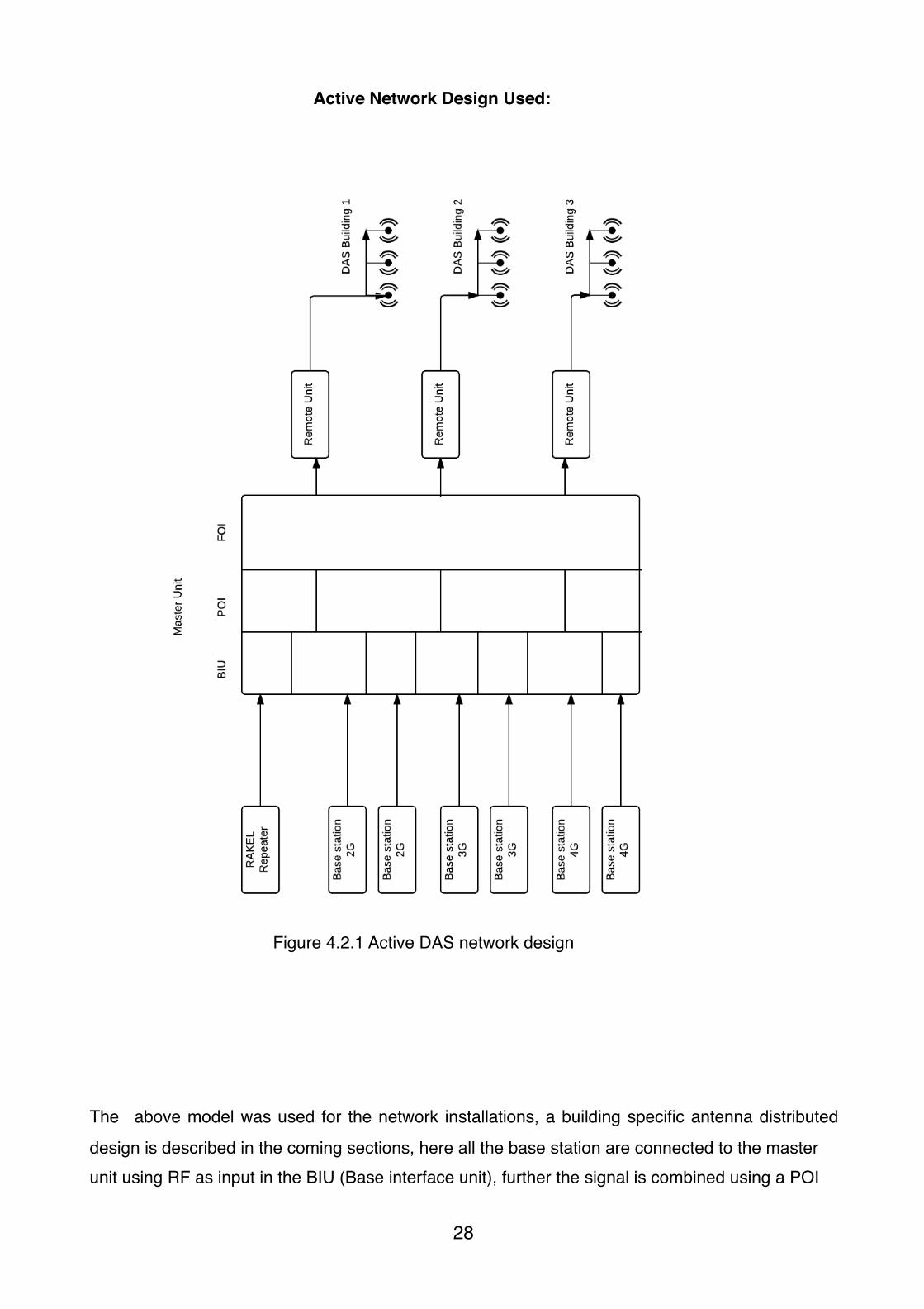
Active Network Design Used:

The above model was used for the network installations, a building specific antenna distributed design is described in the coming sections, here all the base station are connected to the master unit using RF as input in the BIU (Base interface unit), further the signal is combined using a POI

�28

Figure 4.2.1 Active DAS network design

(Power output interface) which acts both as a combiner and splitter. The signal is further sampled and converted using Fiber output interface which feeds the signals to various remote units. At the remote units, output power based on the coverage requirements is configured and then the signal is fed to the antenna system using an RF signal.

4.2.2 Measurement tools

The measurements variable mainly used for the coverage analysis is the RSSI (Received signal strength indication) and as the required RSSI for different radio access is not same, separate measurements have to be taken for this. We also measure the return loss to see and faults in the installation. We cover this using spectrum analyser and TEMS pocket for the coverage analysis and an Anritsu site master for the return loss measurements. The tools description:

Spectrum Analyser:

The spectrum analyser used in this thesis is an ROHDE and SCHWARZ FSH4 spectrum analyser which measures signals ranging from 1 kHz to 3.6 GHz, thus covers all the frequency measurements that we need for the purpose of this thesis. The spectrum analyser has a receiving sensitivity of upto -141 dBm with an accuracy of 0.1 dB [19].

TEMS Pocket:

A samsung galaxy s4 was used with ASCOM TEMS Pocket which a phone based measurement tools to measure the parameter of the wireless network measurements [12] of 2G, 3G and 4G and the result was logged in the form of screen shots.

Site Master

To measure the return loss and the distance to antenna and cable faults measurements an Anritsu site master was used. Cable and antenna systems play an important part in the overall performance of a cellular system.[8] A faulty cable or antenna system is not so easy to replace after the installation phase is over.

Degradation or small changes in cable or antenna system can sometimes result in dropped calls or poor voice quality. A site master test is an excellent indication of the state of cable and antenna.

�29

In the site master test, Frequency Domain Reflectometry is used to locate small degradation and changes in the system to prevent severe system failures.

Return loss and VSWR loss measurements are used to make sure that the costly RF energy is available for transmission with the minimal RF energy reflected back to the transmitter.

Upon detection of return loss in the cable or antenna, Distance-To-Fault (DTF) is used to troubleshoot the system and locate the exact location of the fault.

4.2.3 Measurement locations

For the purpose of coverage analysis three buildings with different structures were used. The buildings are of typical old hospital environment where because of the thickness of the walls the outdoor macro station cannot provide sufficient coverage. Building 1 has been used as the master site location where all the base stations and the master unit have been placed. While building 2 and building 3 has been connected to the master site using a remote unit.

The building and the network description follows:

Building 1/2: Building 1 and 2 are similar other than a basement and has 6 floors and is more new and renovated with 2 corridors:

Floor plan:

�30

Figure 4.2.3.1 Floor Plan Building 1 & 2

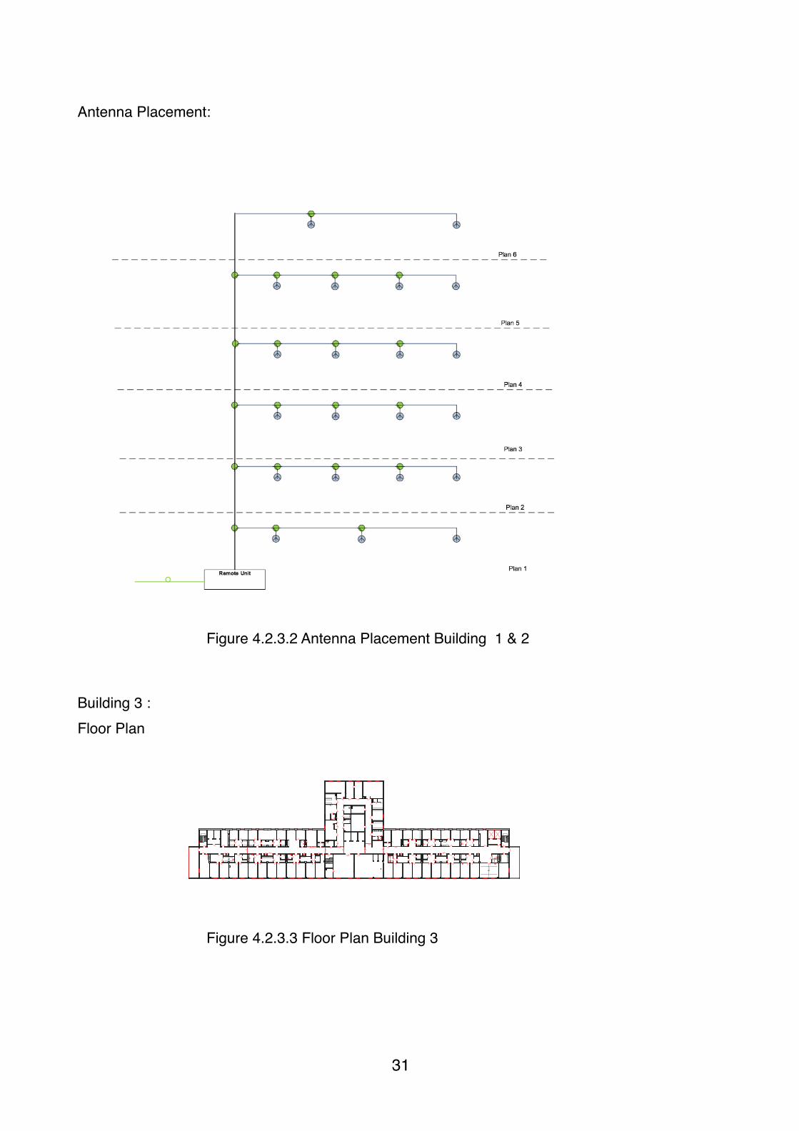
Antenna Placement:

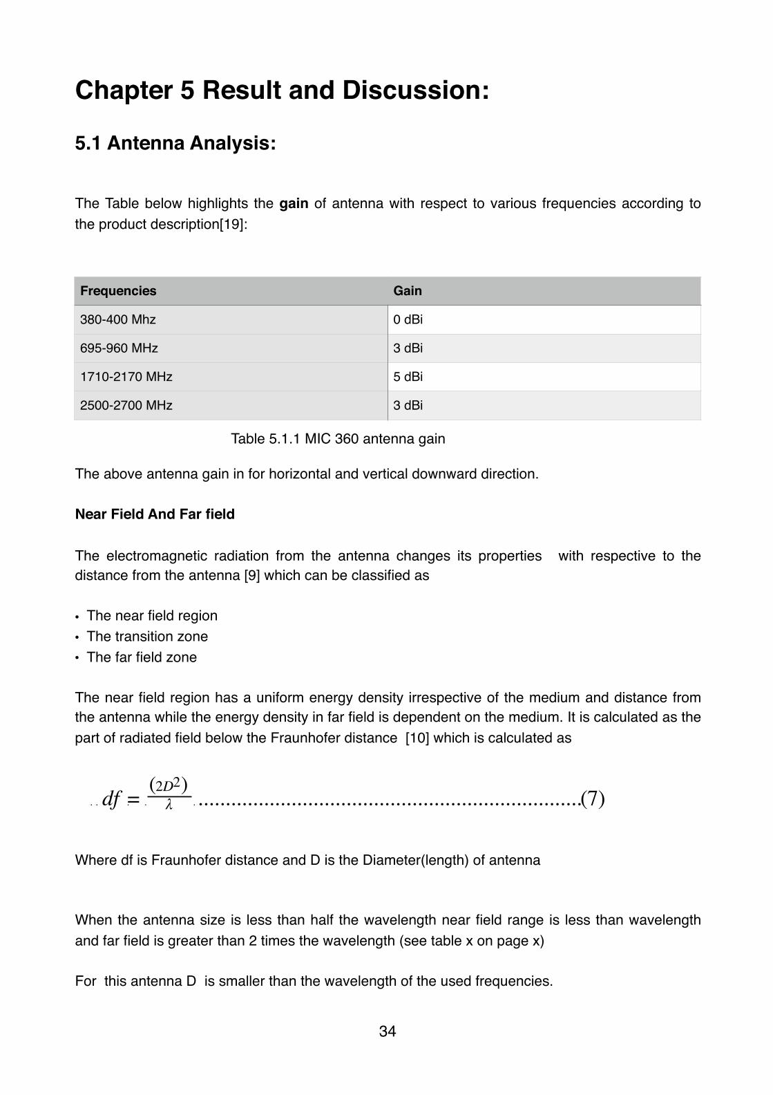
Building 3 :Floor Plan

�31

K/F

MIKRO

KAFFEM.

DM

PATIENTLYFT

PATIENTLYFT

PATIENTLYFT

AV

AVAV

AV

AV

AV

AV

PATIENTLYFT

TS

Figure 4.2.3.2 Antenna Placement Building 1 & 2

Figure 4.2.3.3 Floor Plan Building 3

Building 3 has 11 floors and underground floors and thick walls and contains multiple labs and rooms.

Antenna Design building 3:

�32

Figure 4.2.3.4 Antenna Placement Building 3

4.2.4 Link Budget calculations

For the network design used above, we have to consider that as we are using an active network design with remote units we to calculate the link budget only between remote unit and antennas.Thus the remote unit here will be the transmitter.For the calculations we consider ( UMTS only because of the highest path loss )From remote unit to antenna 1 (farthest antenna from the remote unit): Cable 1/2 Length = 15 m which is 1.65 dB loss (table on page 21)Cable 7/8 Length = 124 m which is 7.192 dB LossTapper and splitters = 17.03 dBTotal losses: 25.872 dB

Note: The network is designed so that all antennas have the same output power. So the losses between the remote unit and antenna is always close to 25 dBm.

By the above loss calculation, the transmitter power should be 25 dBm to neglect lossesThus Transmitter power= 25 dBmLoss = 25.872 dBAntenna gain = 5 dBi

EIRP = Transmitter Power - Loss + Antenna gain = 4.128 dBmBy using the modified path loss in equation 5 (1 wall on average 5 dB) , at 15 meters we get Path loss = 20log(15) + 20log(2100)-27.55 - 5 = 57.416 dB

Link Budget:

Transmitter Output +25 dBmCable + connectors loss -25.872 dBAntenna Tx Gain +5 dBiPath loss (free space + walls) -57.416 dBMiscellaneous losses -10 dBReceiving Sensitivity(UMTS) - 75 dBm (Subtract)

Total 11.72 dB margin

�33

Chapter 5 Result and Discussion:

5.1 Antenna Analysis:

The Table below highlights the gain of antenna with respect to various frequencies according to the product description[19]:

The above antenna gain in for horizontal and vertical downward direction.Near Field And Far field

The electromagnetic radiation from the antenna changes its properties with respective to the distance from the antenna [9] which can be classified as

• The near field region• The transition zone • The far field zone

The near field region has a uniform energy density irrespective of the medium and distance from the antenna while the energy density in far field is dependent on the medium. It is calculated as the part of radiated field below the Fraunhofer distance [10] which is calculated as

Where df is Fraunhofer distance and D is the Diameter(length) of antenna

When the antenna size is less than half the wavelength near field range is less than wavelength and far field is greater than 2 times the wavelength (see table x on page x)

For this antenna D is smaller than the wavelength of the used frequencies.

Frequencies Gain

380-400 Mhz 0 dBi

695-960 MHz 3 dBi

1710-2170 MHz 5 dBi

2500-2700 MHz 3 dBi

�34

Table 5.1.1 MIC 360 antenna gain

The table below mentions the near and far field with respective the different frequencieswhere near field is equal to the wavelength and far field is twice the wavelength

A vector network analyser was used to measure the S parameter for the antenna. To describe S parameters we can consider and electrical system containing two points where point 1 is where the voltage is delivered and point 2 is where it is received. So S12 means the power that is calculated at antenna 2 compared to the power delivers by antenna 1. For this antenna properties, S11 which is the return loss is measured as the reflected power which is delivered by the antenna.

The ratio of power transmitted to the power reflected is measured, the return loss is calculated as

So according to eq 8 if return loss = 0 dB that means Power reflected will be equal to power inserted thus there will be no radiation at all.

Return loss can be converted in reflect power % by calculating the reflection coefficient Γ by:

Frequencies Near Field Transition Zone Far field

380-400 Mhz 72 cm 72 - 140 cm 140 cm

695-960 MHz 32 cm 32-64 cm 64 cm

1710-2170 MHz 16 cm 16-32 cm 32 cm

2500-2700 MHz 11 cm 11-22 cm 22 cm

�35

Table 5.1.2 MIC 360 antenna near and far field

From the below graph we get:

The lower the reflected power, the better the antenna radiation, but a null reflected power can also mean that the antenna is not radiating at that frequency as an antenna with 0 reflected power doesn’t exist.

It can be analysed from the graph that after 2.7 GHz the antenna has an average return loss of 30 % thus It can be used in the frequency range after 2.7 GHz but it will not have the ideal coverage

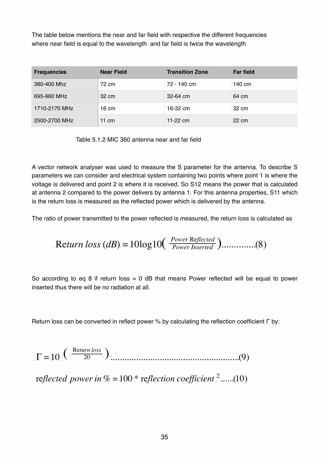
A vector network analyser was used to get the Smith charts for the antenna. Smith chart is a graphical representation for impedance as a function of frequency. Smith chart calculates the complex reflection coefficient

Frequency range (MHz) Loss (dB) Reflection Coefficient Reflected Power %

380-400 6 0.501 25.12

695-960 9 0.355 12.59

1710-2170 14 0.200 3.98

2500-2700 16 0.158 2.51

�36

Figure 5.1.1 S11 MIC 360 antenna

Table 5.1.3 MIC 360 antenna Return loss

0 dB

where Z0 is 50 ohm and ZL is the input impedance

�37

Figure 5.1.3 Smith Chart 800-900 MHz MIC 360 antenna

Figure 5.1.2 Smith Chart 380-490 MHz MIC 360 antenna

�38

Figure 5.1.4 Smith Chart 1800-1900 MHz MIC

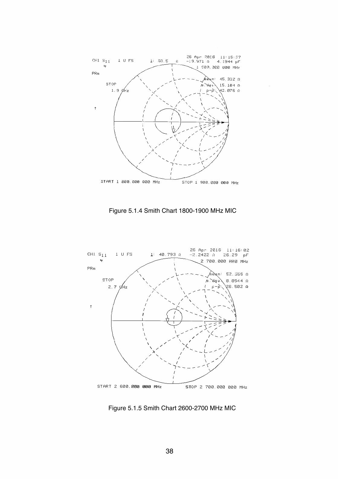
Figure 5.1.5 Smith Chart 2600-2700 MHz MIC

The center of Smith chart has a reflection coefficient as 0 and then the real and imaginary axis is plotted according to the imaginary reflection coefficient.

The first circle in the above graphs represent a reflection coefficient of 2 and 2nd a reflection coefficient of 1 and the 3rd a reflection coefficient of 0.5 and the 4th outermost circle a reflection coefficient of 0. Here we do not consider anything after the reflection coefficient 1 ,as we are not going to get reflected power higher than the transmitted power itself.

And the shift from left to right represent the wavelength towards the generator which is a function of the frequency.

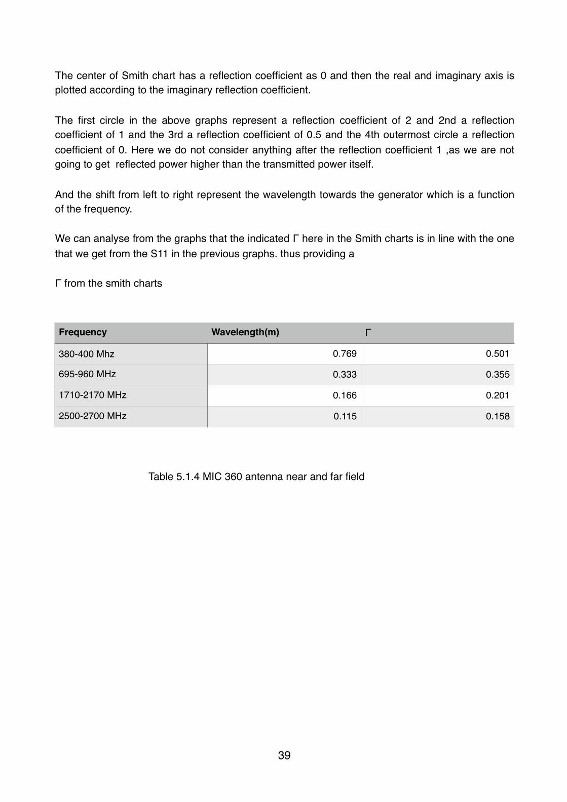
We can analyse from the graphs that the indicated Γ here in the Smith charts is in line with the one that we get from the S11 in the previous graphs. thus providing a

Γ from the smith charts

Frequency Wavelength(m) Γ

380-400 Mhz 0.769 0.501

695-960 MHz 0.333 0.355

1710-2170 MHz 0.166 0.201

2500-2700 MHz 0.115 0.158

�39

Table 5.1.4 MIC 360 antenna near and far field

5.2 Coverage Analysis:

Antenna Location

The buildings have multiple floors and for the purpose of this thesis we have measured the variable at 1 floor in each building.

Antenna locations Building 1 and 3:

For building 1 and 3, 8 antennas are placed at same locations in both buildings.The average distance between antennas is 30 meters.

�40

Figure 5.2.1 Antenna placement building 1 and 2

Antenna Location Building 2

For building 2 there are 8 antennas placed 30 meters from each other, although ideally 7 antennas would be enough for such building design but because of the RF shield in a lab, an extra antenna was required inside the lab.

Measurement Metrics

The key variables normally measured to validate the coverage analysis are

• Return Loss• Signal Strength

For the purpose of this thesis we will only check Return loss and Signal strength as only TETRA and 3G were deployed in the thesis duration and Passive intermodulation does not fall with in the scope of this thesis.

Ideal Case Measurement Metrics.

Return loss: Return loss is measured in dB which is proportional to reflected power back to the system in %. Reflected power can be calculated by:

�41

Figure 5.2.2 Antenna Placement building 3

Using the above equations we get

Return loss dB Reflected Power %

1 79.43

2 63.10

3 50.12

4 39.81

5 31.62

6 25.12

7 19.95

8 15.85

9 12.59

10 10.00

11 7.94

12 6.31

13 5.01

14 3.98

15 3.16

16 2.51

17 2.00

18 1.58

19 1.26

20 0.044

�42

Table 5.2.1 MIC 360 Return loss to Reflected Power

Thus a return loss higher than 14 dB is considered ideal for a network, but in a practical network, a return loss of 10 will be considered ideal.

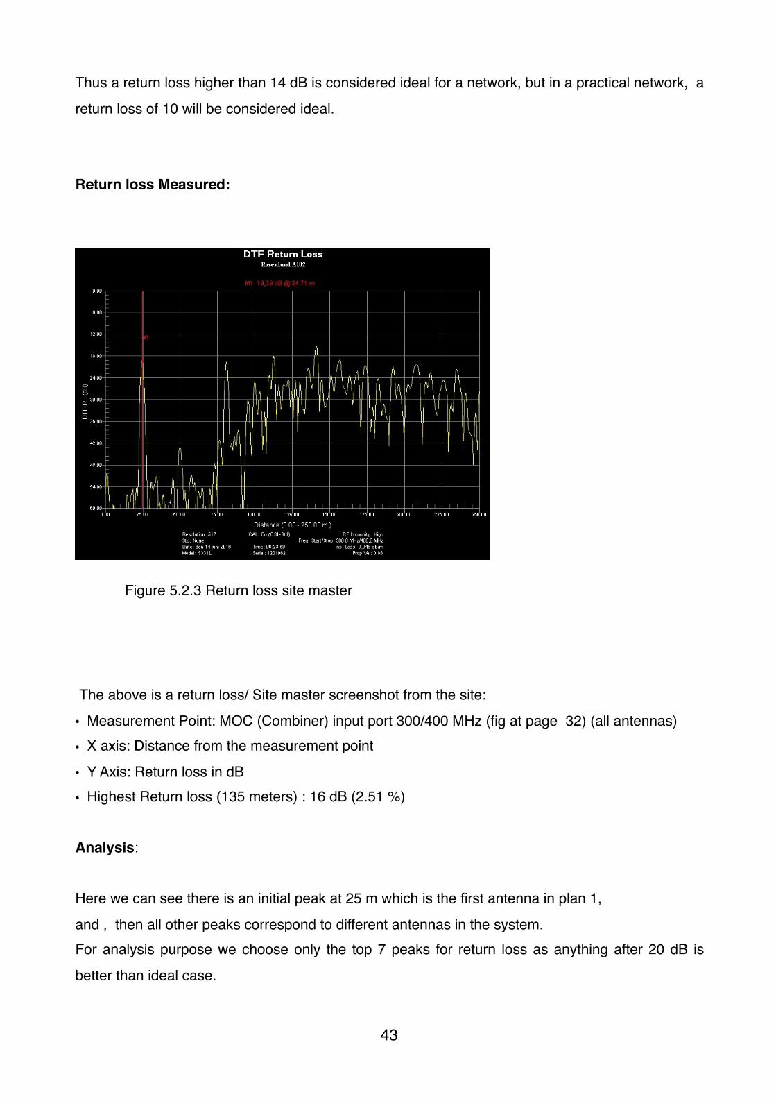
Return loss Measured:

The above is a return loss/ Site master screenshot from the site:

• Measurement Point: MOC (Combiner) input port 300/400 MHz (fig at page 32) (all antennas)• X axis: Distance from the measurement point

• Y Axis: Return loss in dB• Highest Return loss (135 meters) : 16 dB (2.51 %)

Analysis:

Here we can see there is an initial peak at 25 m which is the first antenna in plan 1,and , then all other peaks correspond to different antennas in the system.For analysis purpose we choose only the top 7 peaks for return loss as anything after 20 dB is better than ideal case.

�43

Figure 5.2.3 Return loss site master

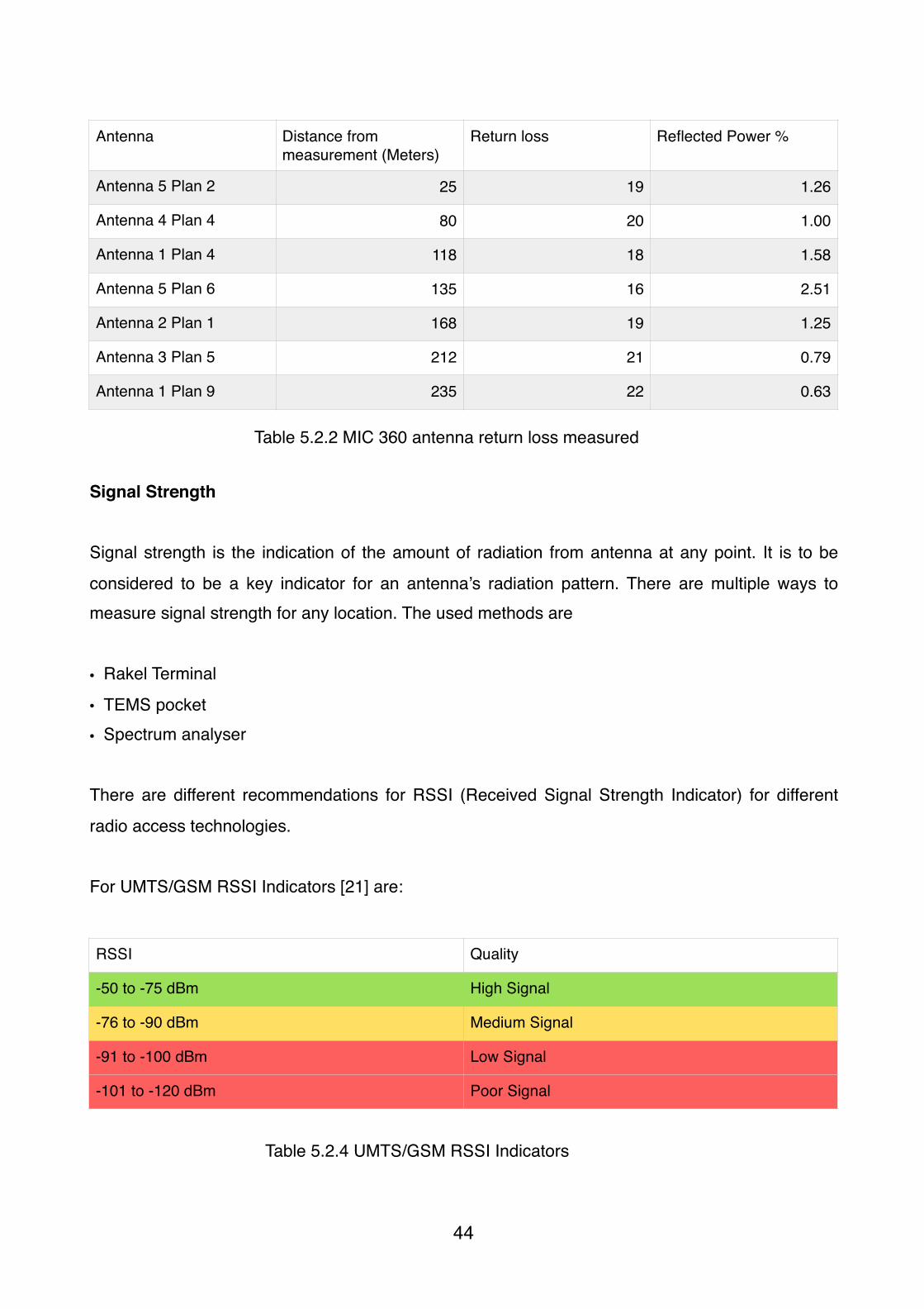
Signal Strength

Signal strength is the indication of the amount of radiation from antenna at any point. It is to be considered to be a key indicator for an antenna’s radiation pattern. There are multiple ways to measure signal strength for any location. The used methods are

• Rakel Terminal

• TEMS pocket

• Spectrum analyser

There are different recommendations for RSSI (Received Signal Strength Indicator) for different radio access technologies.

For UMTS/GSM RSSI Indicators [21] are:

Antenna Distance from measurement (Meters)

Return loss Reflected Power %

Antenna 5 Plan 2 25 19 1.26

Antenna 4 Plan 4 80 20 1.00

Antenna 1 Plan 4 118 18 1.58

Antenna 5 Plan 6 135 16 2.51

Antenna 2 Plan 1 168 19 1.25

Antenna 3 Plan 5 212 21 0.79

Antenna 1 Plan 9 235 22 0.63

RSSI Quality

-50 to -75 dBm High Signal

-76 to -90 dBm Medium Signal

-91 to -100 dBm Low Signal

-101 to -120 dBm Poor Signal

�44

Table 5.2.2 MIC 360 antenna return loss measured

Table 5.2.4 UMTS/GSM RSSI Indicators

For Rakel RSSI Indicators [22] are:

For Coverage analysis of the broadband antenna, we will compare the RSSI for the antenna to that of an Isotropic antenna

Rakel

Ideal Isotropic Antenna:Ideal RSSI is calculated with a power of 0 dBm at the antenna input + antenna gain - Free space path loss 10 meters

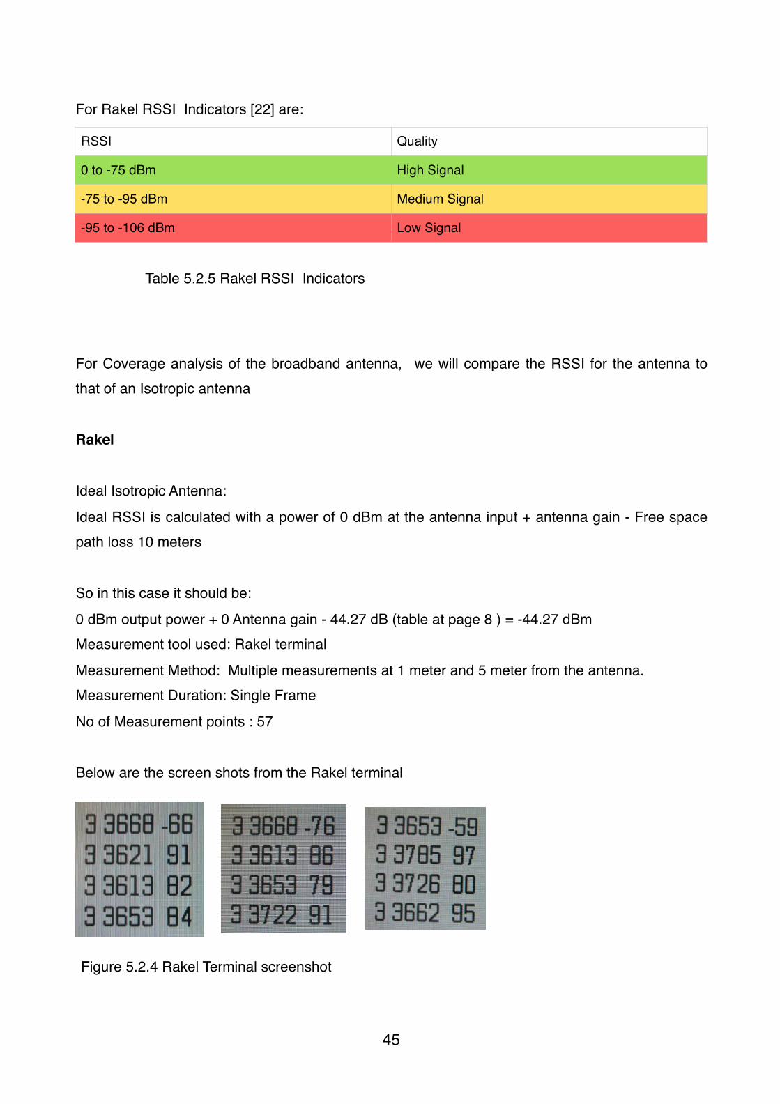
So in this case it should be:0 dBm output power + 0 Antenna gain - 44.27 dB (table at page 8 ) = -44.27 dBmMeasurement tool used: Rakel terminalMeasurement Method: Multiple measurements at 1 meter and 5 meter from the antenna.Measurement Duration: Single FrameNo of Measurement points : 57

Below are the screen shots from the Rakel terminal

RSSI Quality

0 to -75 dBm High Signal

-75 to -95 dBm Medium Signal

-95 to -106 dBm Low Signal

�45

Table 5.2.5 Rakel RSSI Indicators

Figure 5.2.4 Rakel Terminal screenshot

As the RSSI for the isotopic antenna is calculated for free space path loss while the above measurements are for indoor network we can still see that the difference is not significant but falls in the approved category for RAKEL standards [22]

3G/WCDMA

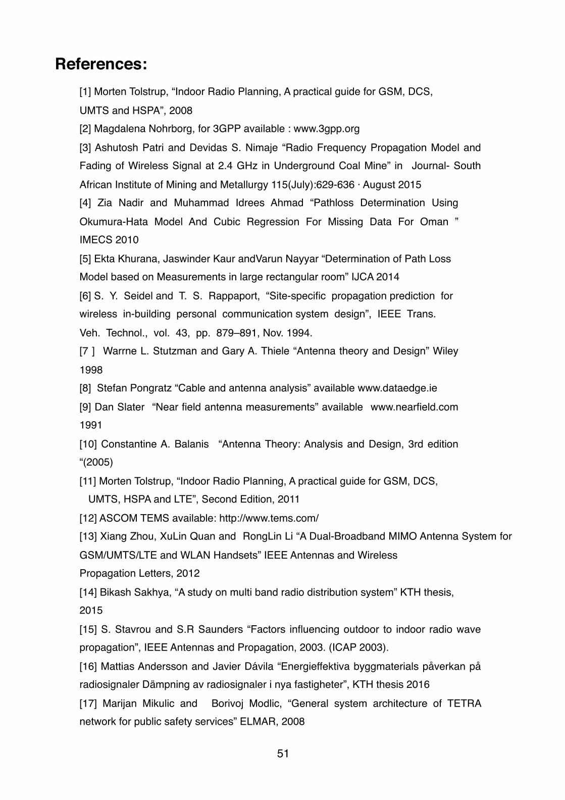
Measurement tools used: TEMS and Spectrum AnalyserMeasurement method: 3 step walking measurements at 5 Meters , 10 meters and 15 meters from the antenna.Measurement duration: Frame measurement.Number of points measured: 53

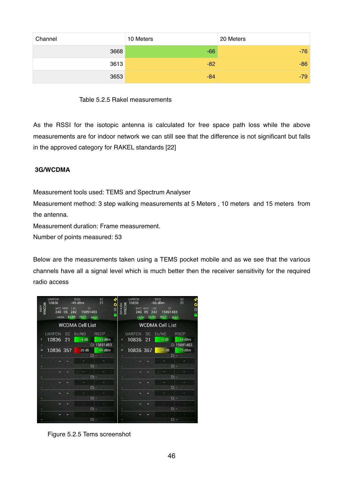
Below are the measurements taken using a TEMS pocket mobile and as we see that the various channels have all a signal level which is much better then the receiver sensitivity for the required radio access

Channel 10 Meters 20 Meters

3668 -66 -76

3613 -82 -86

3653 -84 -79

�46

Figure 5.2.5 Tems screenshot

Table 5.2.5 Rakel measurements

The measurements were taken at 53 locations and the results were averaged for each location with values from 8 meters to 15 meters from the antenna.4 locations had poor coverage i.e less than -92 dBm7 locations have good coverage. i.e greater than -90 dBm 42 locations had an excellent coverage i.e greater than -76 dBmAlso, Spectrum analyser was used at selected location to see if there are and intermodulation and to reconfirm the above measurements. The measurements from TEMS and spectrum analyser are very similar so the results from spectrum analyser have not been listed as the measured RSSI is the same. But for analysis below is a screen shot from the spectrum analyser output for 5 meters from the antenna.

No of Measurements 53

Frequency 2.1 GHz

-50 to -75 dBm 42 Locations

-76 to -90 dBm 7 Locations

-91 to -100 dBm 4 Locations

�47

Table 5.2.6 Spectrum measurements

Table 5.2.5 Spectrum analyser screen shots

Measurement Location: Plan 3 antenna 4.Measurement Tool : R&S FS4 spectrum analyser.Measurement frequency: 2.15 GHzX Axis : Frequency Y Axis : Signal Level in dBmNo of Channels : 4 Distance from antenna: 5 metersFree Space Path loss level: - 52.87 dBm (FSPL at 5 meters) + 5 dBi antenna gain = -47.87 dBmMeasured Value : -56.2 dBm

�48

Chapter 6 Conclusion

The application of a multi band antenna which can cover multiple radio access technologies has been analyzed in this thesis. Radio access technologies including TETRA, 2G, 3G, and 4G from multiple operators has been implemented and deployed for this thesis. Multiple radio equipment and design strategies have been studied and tested for the antenna analysis. The coverage level has been checked across multiple buildings and floors. The investigation of the antenna shows that even though the combined signal from multiple operators is high powered and generally has a possible effect of generating passive intermodulation, but, no such problem has been found with this solution and although the antenna is not proposed to work for WLAN the antenna analysis show that it would also be fit for serving the same. The antenna has a uniform coverage and shows similar signal levels throughout the antenna system. The directivity and radiation pattern of the antenna has been validated using an RF noise free chamber. The antenna has also been measured for 5 GHz WLAN, though having a constant radio pattern and directivity while has a high return loss at 5GHz, the antenna will not be ideal for such frequencies. Because of the high power compatibility up to 15W, the antenna is ideal for a purely active system design with multiple operators and redundant base stations. The coverage was also analyzed, by installing a multiple number of antennas in a live environment and no effect of using the multiple frequencies has been detected in the signal levels. It can be concluded that the wide band antennas can be used to make the network more adaptable with the advancement of the radio access technologies and as it can serve a wide range of frequencies, it might also be suitable for the upcoming radio networks such as coverage for of 2.3 GHz, 2.6 GHz for 5G radio access.

�49

Chapter 7 Future work Although this antenna can cover multitude of radio access technologies there future work related to this thesis can be analysis of a wide band antenna which ideally also covers frequencies upto 5GHz thus also covering wireless 5GHz as generally multiple antennas are placed in an environment used to cover the enter premises, which is an expensive solution if a narrow band antenna is used just for 5GHz compared to a wide band alternative.

�50

References:[1] Morten Tolstrup, “Indoor Radio Planning, A practical guide for GSM, DCS,UMTS and HSPA”, 2008[2] Magdalena Nohrborg, for 3GPP available : www.3gpp.org[3] Ashutosh Patri and Devidas S. Nimaje “Radio Frequency Propagation Model and Fading of Wireless Signal at 2.4 GHz in Underground Coal Mine” in Journal- South African Institute of Mining and Metallurgy 115(July):629-636 · August 2015 [4] Zia Nadir and Muhammad Idrees Ahmad “Pathloss Determination Using Okumura-Hata Model And Cubic Regression For Missing Data For Oman ” IMECS 2010[5] Ekta Khurana, Jaswinder Kaur andVarun Nayyar “Determination of Path Loss Model based on Measurements in large rectangular room” IJCA 2014[6] S. Y. Seidel and T. S. Rappaport, “Site-specific propagation prediction for wireless in-building personal communication system design”, IEEE Trans. Veh. Technol., vol. 43, pp. 879–891, Nov. 1994.[7 ] Warrne L. Stutzman and Gary A. Thiele “Antenna theory and Design” Wiley 1998[8] Stefan Pongratz “Cable and antenna analysis” available www.dataedge.ie[9] Dan Slater “Near field antenna measurements” available www.nearfield.com 1991[10] Constantine A. Balanis “Antenna Theory: Analysis and Design, 3rd edition “(2005) [11] Morten Tolstrup, “Indoor Radio Planning, A practical guide for GSM, DCS, UMTS, HSPA and LTE”, Second Edition, 2011[12] ASCOM TEMS available: http://www.tems.com/ [13] Xiang Zhou, XuLin Quan and RongLin Li “A Dual-Broadband MIMO Antenna System for GSM/UMTS/LTE and WLAN Handsets” IEEE Antennas and Wireless Propagation Letters, 2012 [14] Bikash Sakhya, “A study on multi band radio distribution system” KTH thesis, 2015 [15] S. Stavrou and S.R Saunders “Factors influencing outdoor to indoor radio wave propagation”, IEEE Antennas and Propagation, 2003. (ICAP 2003).[16] Mattias Andersson and Javier Dávila “Energieffektiva byggmaterials påverkan på radiosignaler Dämpning av radiosignaler i nya fastigheter”, KTH thesis 2016[17] Marijan Mikulic and Borivoj Modlic, “General system architecture of TETRA network for public safety services” ELMAR, 2008

�51

[18] Kaaranen, H., Ahtiainen, A., Laitinen, L., Naghian, S. and Niemi, V. (eds) (2005) Front Matter, in UMTS Networks: Architecture, Mobility and Services, Second Edition, John Wiley & Sons, Ltd[19] MIC calculation sheets and database[20] Mardeni R and T.Siva Priya “Optimised COST-231 Hata Models for WiMAX Path Loss Prediction in Suburban and Open Urban Environments ”, Canadian Center of Science and Education September 2010[21] 3GPP RSSI available on ://www.3gpp.org/tsg_ran/WG1_RL1/TSGR1_09/Docs/PDFs/R1-99i82.pdf[22]Rakel Handook available on http://www.forsvarsmakten.se/siteassets/4-om-myndigheten/dokumentfiler/handbocker/handbok-rakel-i-forsvarsmakten.pdf

�52

Appendix A

Table A1: Cable Loss ( Typical )

Table A2 Splitter Loss ( Typical )

Coaxial

Cable

Loss

(dB/100 m)

Loss dB/1 m)

Frequency 1/2" 7/8" 1 1/4" Jumper

400 MHz 4,44 2,35 1,69 0,16

800 MHz 6,41 3,4 2,46

900 MHz 6,95 3,7 2,69 0,3

1800 MHz 9,96 5,3 3,88 0,47

2100 MHz 11 5,8 4,22 0,51

2400 MHz 11,68 6,22 4,58

2600 MHz 12,2 6,45 4,8 0,57

2700 MHz 12,48 6,65 4,91

Splitters Loss (dB) Insertion

Loss (dB)

2-Way -3 0,02

3-Way -4,7 0,02

4-Way -6,25 0,02

�53

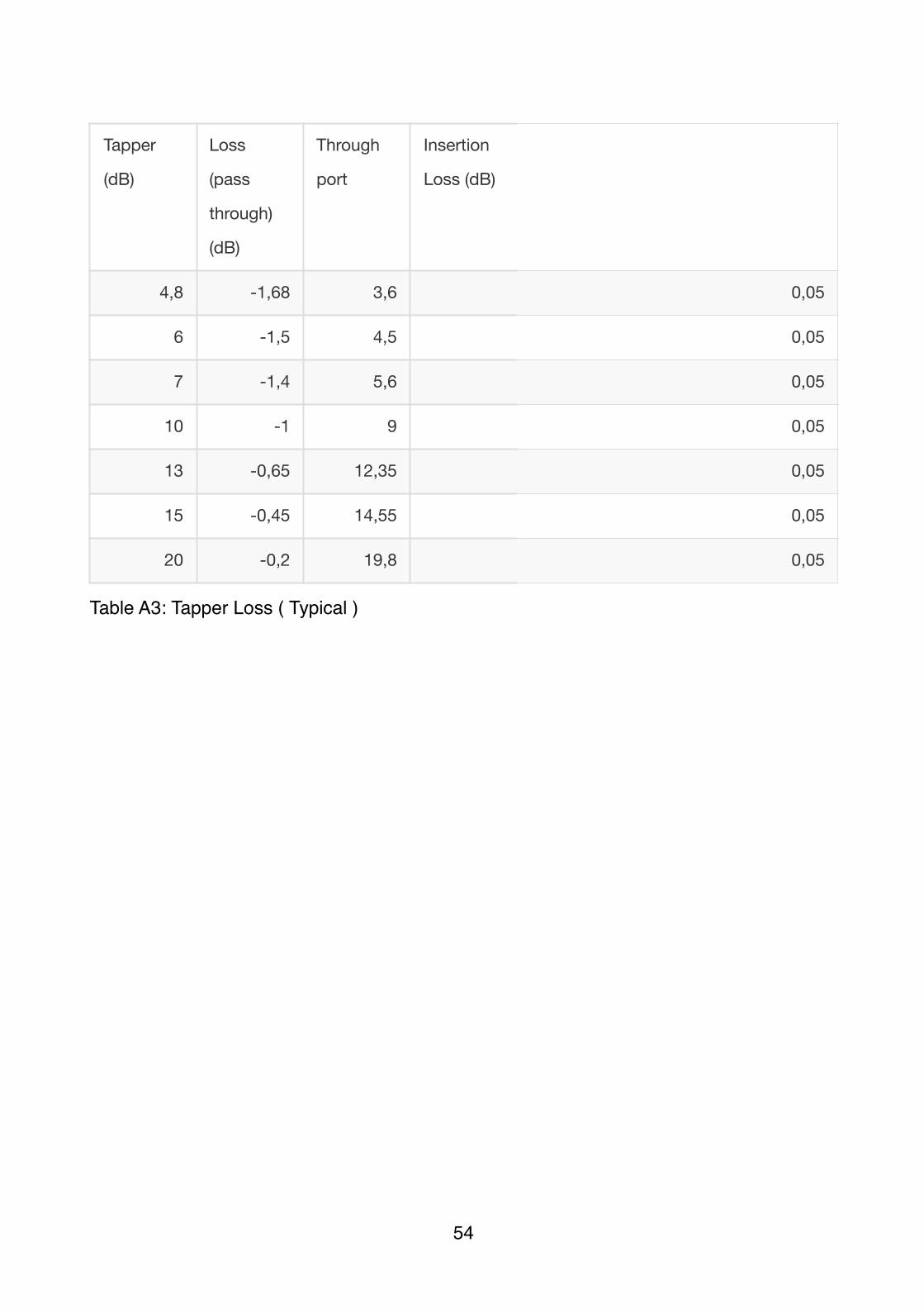
Table A3: Tapper Loss ( Typical )

Tapper

(dB)

Loss

(pass

through)

(dB)

Through

port

Insertion

Loss (dB)

4,8 -1,68 3,6 0,05

6 -1,5 4,5 0,05

7 -1,4 5,6 0,05

10 -1 9 0,05

13 -0,65 12,35 0,05

15 -0,45 14,55 0,05

20 -0,2 19,8 0,05

�54

�55

TRITA TRITA-ICT-EX-2016:143

www.kth.se