Embed Size (px)
Citation preview

A STUDY AND AN IMPLEMENTATION
OF
SCAPEGOAT TREES
Honour Project ReportCarleton University, School of Computer Science
Submitted by Phuong Dao, 100337321Supervised by Dr. Anil Maheshwari
August 15, 2006

ABSTRACT
This report describes the study and implementation of Scapegoat trees, weight andloosely-height-balanced binary search trees, first proposed in the paper:”ScapegoatTrees”[Igal Galperin and Ronald L. Rivest, 1993]. The trees guarantee the amortizedcomplexity of Insert and Delete O(log n) time while the worst case complexity of Searchingis O(log n) time where n is the number of nodes in the tree. It is the first kind of balancedbinary search trees that do not store extra information at every node while still maintainingthe complexity as above. The values kept track are the number of nodes in the tree and themaximum number of nodes since the trees were last rebuilt. The name of the trees comesfrom that rebuilding the tree only is taken place only after detection of a special node calledScapegoat, whose rooted subtree is not weight-balanced. In this report, the correctness andcomplexity of operations on Scapegoat trees will be thoroughly and mainly discussed. Also,the test cases from Demo on the operations will be presented. Finally, an application oftechniques used in Scapegoat trees will be discussed and conclusions will be drawn.
i

ACKNOWLEDGEMENTS
I would like to thank very much to Dr. Anil Maheshwari for his guidance and en-thusiasm not only in supervising my project but also in inspiring me to further study inComputer Science and the most to my parents and my sister who always support me andbe there for me.
ii

Contents
1 INTRODUCTIONS 3
1.1 Binary Search Tree Notations . . . . . . . . . . . . . . . . . . . . . . . . . . 31.2 Weight Balanced Binary Search Tree . . . . . . . . . . . . . . . . . . . . . . 41.3 Height Balanced Binary Search Tree . . . . . . . . . . . . . . . . . . . . . . 61.4 Scapegoat Tree Related Definitions . . . . . . . . . . . . . . . . . . . . . . . 6
2 OPERATIONS ON SCAPEGOAT TREES 8
2.1 How to search for a key . . . . . . . . . . . . . . . . . . . . . . . . . . . . . . 92.2 How to insert a new key . . . . . . . . . . . . . . . . . . . . . . . . . . . . . 92.3 How to delete a key . . . . . . . . . . . . . . . . . . . . . . . . . . . . . . . . 112.4 Rebuild Scapegoat Subtree . . . . . . . . . . . . . . . . . . . . . . . . . . . . 11
3 CORRECTNESS 15
3.1 Main Theorem . . . . . . . . . . . . . . . . . . . . . . . . . . . . . . . . . . 153.2 Insert . . . . . . . . . . . . . . . . . . . . . . . . . . . . . . . . . . . . . . . 163.3 Delete . . . . . . . . . . . . . . . . . . . . . . . . . . . . . . . . . . . . . . . 17
4 TIME COMPLEXITY 19
4.1 Find Scapegoat and Rebuild . . . . . . . . . . . . . . . . . . . . . . . . . . . 194.2 Search . . . . . . . . . . . . . . . . . . . . . . . . . . . . . . . . . . . . . . . 204.3 Insert . . . . . . . . . . . . . . . . . . . . . . . . . . . . . . . . . . . . . . . 204.4 Delete . . . . . . . . . . . . . . . . . . . . . . . . . . . . . . . . . . . . . . . 214.5 Generalized Theorem . . . . . . . . . . . . . . . . . . . . . . . . . . . . . . . 22
5 APPLICATION 23
5.1 Orthogonal range queries . . . . . . . . . . . . . . . . . . . . . . . . . . . . . 23
6 CONCLUSIONS AND FUTURE WORK 25
6.1 Conclusions . . . . . . . . . . . . . . . . . . . . . . . . . . . . . . . . . . . . 256.2 Future Work . . . . . . . . . . . . . . . . . . . . . . . . . . . . . . . . . . . . 25
REFERENCES 27
A HOW TO USE THE DEMO 28
A.1 How to run . . . . . . . . . . . . . . . . . . . . . . . . . . . . . . . . . . . . 28A.2 How to do Search, Insert, and Delete . . . . . . . . . . . . . . . . . . . . . . 28
1

A.3 How to reset tree with a new α . . . . . . . . . . . . . . . . . . . . . . . . . 28
B LIST OF FIGURES AND TABLES 32
2

Chapter 1
INTRODUCTIONS
There are two main balanced binary search tree schemes: height-balanced and weight-balanced. The height-balanced scheme maintains the height of the whole tree in O(log n)where n is the number of nodes in the tree. Red-black trees by Bayer [1], Guibas andSedgewick [4] and AVL trees are examples of this scheme in which the worst-case cost ofevery operation is O(log n) time. The weight-balanced scheme ensures the size of subtreesrooted at siblings for every node in the tree approximately equal. Nievergelt and Reingold[6] first introduced a tree using such scheme to implement Search and Update operations inO(log n) time as well. The technique used in Scapegoat trees combines those two schemes.By maintaining weight-balanced, it also maintains height-balanced for a Search operationand by detecting a height-unbalanced subtree and rebuilding the subtree, it also ensuresweight-balanced after an update operation. Before going deep into operations in Scapegoattrees, let’s get ourselves familiar with notations and definitions of balanced binary searchtrees.
1.1 Binary Search Tree Notations
If n is a node in a Scapegoat tree T then
• n.key is the value of the key stored at the node n
• n.left refers to the left child of n
• n.right refers to the right child of n
• n.height refers to the height of the subtree rooted at n or the longest distance in termsof edges from n to some leaf.
• n.depth refers to the depth of node n or the distance in terms of edges from the rootto n
• n.parent refers to the parent node of node n
• n.sibling refers to the other child, other than n, of parent of n
3

5
2 8
960
7
Figure 1.1: A binary search tree with α = 0.6
• n.size refers to the number of nodes of subtree rooted at n. This notation is used forproofs of correctness and time complexity
• n.hα is computed as n.hα = ⌊log1/α (n.size)⌋
• n.size() is the procedure to compute the size of the binary search tree rooted at noden. This notation is used in the descriptions of operations on Scapegoat trees.
What is in bold font, for example n.key, is what is really stored at each node. The others,except for the procedures, are just values used for discussions in proofs of correctness andtime complexity of operations on Scapegoat trees. Below are notations related to a binarysearch tree T :
• T.root refers to the root of the tree T
• T.size refers to the current number of nodes in the tree T
• T.maxSize refers to the maximum number of nodes or the maximum number of T.sizeis or was since T was completely rebuilt because whenever the whole tree T is rebuilt,T.maxSize is set to T.size
• T.hα is computed as following: T.hα = ⌊log1/α (T.size)⌋
• T.height refers to the height of T or the longest path in terms of edges from T.root tosome leaf in T
Similar to notations of a node, what is in bold font is what is stored in tree T . T.height isjust used in concepts and proofs.
1.2 Weight Balanced Binary Search Tree
Definition 1.2.1. A node n in a binary search tree is α-weight-balanced for some α suchthat 1/2 ≤ α < 1 if (n.left).size ≤ α · n.size and (n.right).size ≤ α · n.size.
4

Table 1: Examples of notations for a binary tree node 8 in Figure 1.1
n.key n.parent n.sibling n.left n.right n.height n.depth n.size n.hα n.size()8 5 2 6 9 2 1 4 2 4
Table 2: Examples of notations for a binary search tree in Figure 1.1
T.root T.size T.height T.hα
5 7 3 3
7
5
3 6
8
9
10
Figure 1.2: A weight-unbalanced binary search tree with α = 0.6
5

5
3 7
8
9
6
Figure 1.3: A height-unbalanced binary search tree with α = 0.55
Example 1.2.1. Node 8 in Figure 1.2 is not 0.6-weight-balanced because its right subtreehas 2 nodes which is greater than 0.6∗3 = 1.8 where 3 is the total nodes of the subtree rootedat 8.
Definition 1.2.2. A binary search tree T is α-weight-balanced for some α such that 1/2 ≤α < 1 if all of its nodes are α-weight-balanced.
Example 1.2.2. The tree in Figure 1.2 is not 0.6-weight-unbalanced binary search treebecause it contains node 8 which is not 0.6-weight-balanced.
1.3 Height Balanced Binary Search Tree
Definition 1.3.1. A binary search tree is α-height-balanced for some α such that 1/2 ≤ α <1 if T.height ≤ T.hα.
Example 1.3.1. The tree in Figure 1.2 is 0.6-height-balanced binary search tree because ithas 7 nodes and its height is 3 ≤ ⌊log1/0.6 (7)⌋ = 3.
1.4 Scapegoat Tree Related Definitions
Definition 1.4.1. A node n in a binary search tree T is a deep node for some α such that1/2 ≤ α < 1 if n.depth > T.hα.
Definition 1.4.2. A node s is called Scapegoat node of a newly inserted deep node n if sis an ancestor of n and s is not α-weight-balanced.
Example 1.4.1. If we have just inserted node 9 into the tree T in Figure 1.3 then node 9is a deep node because its height is 3 which is greater than T.hα = ⌊log1/0.55 (6)⌋ = 2. Andin this case, root 5 would be chosen as Scapegoat node.
6

7
5
3 6
9
10
Figure 1.4: An incomplete binary search tree
Definition 1.4.3. A binary search tree is loosely α-height-balanced for some α such that1/2 ≤ α < 1 if T.height ≤ (T.hα + 1).
Example 1.4.2. The tree T in Figure 1.3 is a good example of loosely 0.55-height-balancedwith 3 = T.height ≤ (T.hα + 1) = (⌊log1/0.55 (6)⌋ + 1) = 3
Definition 1.4.4. A binary search tree T is complete if inserting any node into T increasesits height.
Example 1.4.3. The tree in Figure 1.4 is incomplete. But after inserting node 8 into thetree, it becomes complete.
With all the above definitions, we could now envision the notion of a Scapegoat tree. AScapegoat tree is just a regular binary search tree in which the height of the tree is alwaysloosely α-height-balanced. Such balance is maintained after an Insert operation of a deepnode or a Delete operation that leads to T.size < α · T.maxsize. In the case of insertinga deep node, a Scapegoat node s will be detected. Both cases will result in rebuilding thesubtree rooted at s into a 1/2-weight-balanced binary search one.
7

Chapter 2
OPERATIONS ON SCAPEGOAT
TREES
This chapter will present how to do Search, Insert, Delete operations on a Scapegoat tree.An update i.e. Insert or Delete will come with an example which is taken out from the Demofor this project. So before going deep into the operations, let’s take a look at a Scapegoattree from Demo:
Figure 2.1: A sample Scapegoat tree from the Demo
Figure 2.1 presents a Scapegoat tree T with α = 0.57 of size 7, hα = 3 and T hadsize(maxSize) 8 before node 10 was just deleted. These three indexes are at the top ofthe tree. Notice that for each node in T , there are also three indexes surrounding it. Theindex prefixed by s is the size of the subtree rooted at that node while the one prefixed by his the height of the node in T . The index prefixed by ha below each node is the hα of thatnode.
8

2.1 How to search for a key
The Search operation in Scapegoat tree T is done like regular Search in a binary search tree.As we will prove later that the height of a Scapegoat tree T is always loosely-height-balancedin term of the number of nodes T.size after Insert or Delete operations or T.height <⌊log1/α (T.size)⌋ + 1 then worst-case running time is O(log (T.size)) time. Below is thesimple recursive procedure Search:
Procedure 2.1.1 Search(root, k)
Input: root is the root of some tree T to search for an integer key kOutput: n is a node in T such that n.key = k or null if there is no such n1: if root = null or root.key = k then
2: return root3: else if k ≤ root.left.key then
4: return Search(root.left, k)5: else
6: return Search(root.right, k)7: end if
2.2 How to insert a new key
The Insert in Scapegoat tree T is also done like the regular Insert operation in a binarysearch tree when T is still height-balanced. When T is not height-balanced then by MainTheorem (3.1.1), a Scapegoat node s will be detected and rebuilding will be taken place atthe subtree rooted at s. Proof of the Main Theorem also shows how to find the Scapegoatgiven newly inserted node n that makes T height-unbalanced. The Scapegoat s will be thefirst ancestor of n such that s.height > s.hα. The procedure FindScapegoat(n) implementedin the following will return the Scapegoat s giving the newly inserted deep node n:
After the Scapegoat s is detected if applicable, the procedure RebuildTree(size, root) willget called. RebuildTree will rebuild a new 1/2-weight-balanced subtree from the subtreerooted at Scapegoat node returned. Details of procedure RebuildTree will be presented inthe rebuilding section. The Insert procedure also makes use of InsertKey(k) which is amodified version of regular insertion in a binary search tree that will return the height forthe newly inserted node for comparison with T.hα to detect whether a newly inserted nodeis a deep node or not:
Example 2.2.1. Figure 2.2 shows a Scapegoat tree T with α = 0.57 before inserting node29. If node 29 is inserted, it would be the right child of node 22 and because the height of thetree is 4 > T.hα = 3 then node 29 is a deep node. Scapegoat node 8 will be detected and thewhole tree T will be rebuilt into 1/2-weight-balanced binary search tree in Figure 2.3.
9

Procedure 2.2.1 FindScapegoat(n)
Input: n is a node and n 6= null
Output: A node s which is a parent of n and is a Scapegoat node1: size = 12: height = 03: while (n.parent <> null) do
4: height = height + 15: totalSize = 1 + size + n.sibling.size()6: if height > ⌊log1/α(totalSize)⌋ then
7: return n.parent8: end if
9: n = n.parent10: size = totalSize11: end while
Figure 2.2: A Scapegoat tree before insertion
Figure 2.3: A Scapegoat tree after insertion
10

Procedure 2.2.2 Insert(k)
Input: The integer key kOutput: true if the insertion is successful, false if there exists a node n such that n.key = k1: height = InsertKey(k)2: if height = −1 then
3: return false;4: else if height > T.hα then
5: scapegoat = FindScapegoat(Search(T.root, k))6: RebuildTree(n.size(), scapegoat)7: end if
8: return true
2.3 How to delete a key
Deleting a node in a Scapegoat tree T is done by first deleting the node in a regular binarysearch tree then compare T ’s current size(T.size) to T ’s maximum size(T.maxSize) that Tobtained since its latest total rebuilding. If T.size < α ∗ T.maxSize (1) then the whole treeT will be rebuilt into 1/2-weight-balanced binary search tree and T.maxSize = T.size. Theintuition behind that is when (1) is satisfied, T might not be α-weight-balanced so it mightnot be loosely α-height-balanced either. But we need to maintain T α-height-balanced orloosely α-height-balanced then T needs to be rebuilt.
Procedure 2.3.1 Delete(k)
Input: The integer key kOutput: There is no node n in T such that n.key = k1: deleted = DeleteKey(k)2: if deleted then
3: if T.size < (T.α · T.maxSize) then
4: RebuildTree(T.size, T.root)5: end if
6: end if
Example 2.3.1. Figure 2.4 shows a Scapegoat tree before a series of deletions of node 9,10, 16 with α = 0.57. As seen, the tree is still 0.57-height-balanced but after the series ofdeletion it is loosely 0.57-height-balanced but not 0.57-height-balanced in Figure 2.5. But ifwe remove one more node, node 1, the whole tree would be rebuilt into 1/2-weight-balancedin Figure 2.6.
2.4 Rebuild Scapegoat Subtree
The procedures below are basically the same as the procedures of rebuilding 1/2-weight-balanced tree in the original paper :”Scapegoat Trees”[Igal Galperin and Ronald L. Rivest,1993] [3] but with adaptation to my notations and an elimination of a dummy variable.
11

Figure 2.4: A Scapegoat tree before series of deletion
Figure 2.5: A Scapegoat tree after series of deletions
Figure 2.6: A Scapegoat tree after series of deletions and rebuilding
12

The procedures are presented here because later I will provide proofs of time complexity ofrebuilding procedures which are not clearly mentioned in the original paper. The idea ofrebuilding 1/2-weight-balanced tree is straight. First flatten tree into the list of nodes innondecreasing order of their keys. Then divide the list into three parts, among which the listof first half number of nodes and the second half number of nodes will be recursively rebuiltinto 1/2-weight-balanced trees and the new root would be the middle node. Its left subtreeis the 1/2-weight-balanced tree returned from recursive call for first half list of nodes. Itsright subtree is the 1/2-weight-balanced tree returned from recursive call for second half listof nodes. The procedure Flatten Tree(root, head) will return the list of nodes of a binarysearch tree rooted at root in nondecreasing order of their keys appending by the list headedby a node head. The nodes in the list returned are linked by the right fields:
Procedure 2.4.1 Flatten Tree(root, head)
Input: root is the root of some tree TOutput: The list of all nodes in T in nondecreasing order in terms of their keys headed by
node head. The node that contains the smallest key in the tree T will be returned.1: if root = null then
2: return head3: end if
4: root.right = Flatten Tree(root.right, head)5: return Flatten Tree(root.left, root)
The procedure Build Height Balanced Tree(size, head) will build a 1/2-weight-balancedtree from the flatten list of all the nodes in a binary search tree T . The procedure will returnthe last node of the flatten list. Now, the procedure Rebuild Tree(size, scapegoat) justmakes use of Flatten Tree(root, head) procedure to flatten the subtree rooted at scapegoatand Build Height Balanced Tree(size, head) to rebuild the flatten list into 1/2-weight-balanced binary search tree T . Because the call Build Height Balanced Tree(size, head)will return the last node of the flatten list so in order to retrieve the root of the 1/2-weight-balanced tree then just traverse the parents of node head until we reach the root and thiscould be done in O(log (T.size)) time because T is 1/2-weight-balanced then T is also 1/2-height-balanced.
13

Procedure 2.4.2 Build Height Balanced Tree(size, head)
Input: The list of size nodes in nondecreasing order in terms of their keys headed by nodehead
Output: A 1/2-weight-balanced tree built from the list above. The last node of the list willbe returned.
1: if size = 1 then
2: return head3: else if size = 2 then
4: (head.right).left = head5: return head.right6: end if
7: root = (Build Height Balanced Tree(⌊(size − 1)/2⌋, head)).right8: last = Build Height Balanced Tree(⌊(size − 1)/2⌋, root.right)9: root.left = head
10: return last
Procedure 2.4.3 Rebuild Tree(size, scapegoat)
Input: A scapegoat node scapegoat that is the root of a subtree of size nodesOutput: A 1/2-weight-balanced subtree built from all the nodes of the subtree rooted at
scapegoat. The root of the rebuilt subtree will be returned1: head = Flatten Tree(scapegoat,null)2: Build Height Balanced Tree(size, head)3: while head.parent!=null do
4: head = head.parent5: end while
6: return head
14

Chapter 3
CORRECTNESS
3.1 Main Theorem
Theorem 3.1.1. If T is an α-weight-balanced binary search tree, then T is α-height-balancedas well.
Proof. We could prove the other way around: If T is not α-height-balanced then T is notα-weight-balanced either. If T is not α-height-balanced then there is node n0 such thatn0 > T.hα (2). Denote the deepest ancestor of n0 which is not α-height-balanced as ni orlet n1, ..., ni be ancestors of n0 such that n1 is the parent of n0 and so on, then ni is the firstancestor of n0 that satisfies (2). Such ni always exists because T.root always satisfies (2).By the way of choosing such ni, the following inequalities are satisfied:
i > ni.hα
⇒ i > ⌊log1/α (ni.size)⌋⇒ i > log1/α (ni.size)
(3)
andi − 1 ≤ ni−1.hα
⇒ i − 1 ≤ ⌊log1/α (ni−1.size)⌋⇒ i − 1 ≤ log1/α (ni−1.size)⇒ 1 − i ≥ − log1/α (ni−1.size)
(4)
(3) + (4) gives1 > log1/α (ni.size) − log1/α (ni−1.size)
⇒ 1 > log1/α
ni.size
ni−1.size
Due to 12≤ α < 1 or
1
α> 1 and ni.size > ni−1.size
Thenni−1.size > α · ni.size
Therefore, the node ni is not α-weight-balanced or T is not α-weight-balanced.
15

The proof above shows us not only how to find the Scapegoat node s for rebuilding thesubtree rooted at s when a deep node n is detected but also such node s always exists. Letd be the distance in term of edges from n to s, s is the deepest ancestor of n such thatd > s.hα.
3.2 Insert
Lemma 3.2.1. A 1/2-weight-balanced binary search tree T has the smaller than or equalheight of any binary search tree T ′ of the same size.
Proof. First notice that
⌊log2(T′.size)⌋ ≤ T ′.height
⇒ ⌊log2(T.size)⌋ ≤ T ′.height
Due to T.size = T ′.sizeAnd by Main Theorem (3.1.1), T is 1/2-height-balanced:
T.height ≤ ⌊log2(T.size)⌋
Therefore,T.height ≤ T ′.height
Lemma 3.2.2. If T.root is not α-weight-balanced node then its heavy subtree contains atleast 2 more nodes than its light subtree.
Proof. Denote the sizes of the heavy, light subtrees of the root, and the whole tree by h,l,and t, respectively. We have:
h + l + 1 = t
andh > α · t
⇒ h > α · (h + l + 1)⇒ h · (1 − α) > α · l + α
⇒ h ·1 − α
α> l + 1
Since 1/2 ≤ α < 1 or 1 < 1α≤ 2 and 0 < 1 − α ≤ 1/2 then 1−α
α< 1.
Therefore,
h > h ·1 − α
α> l + 1
and h and l are positive integers then h ≥ l + 2
Lemma 3.2.3. If T is not α-weight-balanced and T contains only one node at depth T.heightthen rebuilding T decreases its height.
16

Proof. Let n be the only node at depth T.height. Let T ′
l , T ′
h be the light and heavy subtreesof a subtree T ′ rooted at Scapegoat node s which is α-weight-unbalanced and is an ancestorof n, by proof of Main Theorem (3.1.1), s always exists. If n ∈ T ′
l then T ′ after removing nis not complete tree of height T ′.height − 1 because T ′
h contains at least 2 more nodes thanT ′
l by Lemma(3.2.2) but T ′
h.height < T ′
l .height. In the other case n /∈ T ′
l or n ∈ T ′
h, T ′ isstill not complete subtree of height T ′
l .height − 1 after removing n because T ′
h has at least2 more nodes than T ′
l but T ′
h.height > T ′
l .height. So rebuilding tree T results in rebuildingT ′ into 1/2-weight-balanced binary search tree that causes it decrease its height by Lemma(3.2.1) or T decreases its height.
Theorem 3.2.4. If a Scapegoat tree T was created from a 1/2-weight-balanced tree by asequence of Insert operations then T is α-height-balanced.
Proof. This proof is done by induction. If there are no Insert operations then by MainTheorem (3.1.1), the theorem follows. Suppose that it is true that if a Scapegoat tree Twas created from a 1/2-weight-balanced tree by any sequence of n Insert operations thenT is α-height-balanced. We have to prove it also holds for an extra Insert done after thosesequences. If the extra Insert does not cause T to rebuild, T is still α-height-balanced becauseit was and the height of newly inserted node is not over T.hα. If the extra Insert does causeT to rebuild or the depth of the newly inserted node n: n.depth > T.hα and n is the onlynode at depth T.hα + 1 then by Lemma (3.2.3), the theorem is followed.
3.3 Delete
Lemma 3.3.1. Let T be a α-weight-balanced binary search tree and let T’ be the tree afterinserting a node n into T then T ′.height ≤ max(T ′.hα, T.height)
Proof. If rebuilding is not triggered after the insertion of n, then the depth of n is at mostT ′.hα or T ′.height ≤ T ′.hα or T ′.height ≤ max(T ′.hα, T.height). If the insertion of n causesT to rebuild or n.depth > T ′.hα, there are still two cases to take care. In first case where therewere already some other nodes at n.depth, since rebuilding tree into 1/2-weight-balanced doesnot make the tree deeper by Lemma (3.2.1) or T ′.height ≤ T.height ≤ max(T ′.hα, T.height).In the other case where n is the only node at n.depth > T ′.hα, by Lemma (3.2.3), rebuildingtree does not make the tree deeper, we’re done.
Lemma 3.3.2. Let T be a loosely α-height-balanced binary search tree such that T.height =T.hα + 1 and let T ′ be the tree after insert a node n into T such that T ′.hα = T.hα + 1 thenT ′ is α-height-balanced.
Proof. We have
T.height = T.hα + 1T ′.hα = T.hα + 1
thenT.height = T ′.hα
17

Then Lemma (3.3.1) gives
T ′.height ≤ max(T ′.hα, T.height)⇒ T ′.height ≤ max(T ′.hα, T ′.hα)⇒ T ′.height ≤ T ′.hα
Therefore, T’ is α-height-balanced by Definition (1.3.1),
Lemma 3.3.3. A Scapegoat tree T built from a sequence of Insert and Delete operationsfrom an empty tree is always loosely α-height-balanced.
Proof. Divide the sequence of Insert and Delete operations into subsequences of consecutiveoperations o1, ..., ok such that at the end of each sequence the tree has to be rebuilt and duringthe executions of operations, no rebuilding is taken place. So we need to show that duringsuch sequence of operations, the tree is α-height-balanced or loosely α-height-balanced.In the case that during any sequence of Insert and Delete operations, if T.hα does notchange then max(T.hα, T.height) is not increased and the tree is still at least loosely α-height-balanced. This is because Delete operation could not increase max(T.hα, T.height)nor the Insert operation:Let T ′ be the tree after inserting a node into T which is a tree after an operation oi (1 ≤ i ≤ k)in the sequence. Now we have to prove that max(T ′.hα, T ′.height) ≤ max(T.hα, T.height).By Lemma (3.3.1):
T ′.height ≤ max(T ′.hα, T.height)⇒ max(T ′.hα, T ′.height) ≤ max(T ′.hα, T.height)⇒ max(T ′.hα, T ′.height) ≤ max(T.hα, T.height)
In the other case, T.hα is changed during sequence of Insert and Delete operations. Denoteo′1, ..., o
′
l be the sequence of operations that change T.hα and let T ′ be the tree after insertinga node into T which is a tree before some operation o′i (1 ≤ i ≤ l). For an Insert operation,if T is α-height-balanced then T ′ is loosely α-height-balanced because T.hα is increased atmost 1 and the same for T.height. Otherwise if T is loosely α-height-balanced but not α-height-balanced, by Lemma (3.3.2), T’ is α-height-balanced. For a Delete operation, noticethat there are no two consecutive Delete operations in that sequence. This is due to if aDelete operation change T.hα, it will decrease T.hα by 1 or the cutting size is α ·T.maxSize.If there is another Delete operation right, and we know the second will again cause T.hα
decrease by 1 then rebuilding should be taken between those two Delete operations. Thisviolates our assumption. So a Delete operation should be performed on α-height-balancedtree. As we know a Delete operation does not increase T.height nor Tα then the tree afterwill be at most loosely α-height-balanced. This completes the proof.
18

Chapter 4
TIME COMPLEXITY
4.1 Find Scapegoat and Rebuild
Theorem 4.1.1. The time to find the Scapegoat node s is O(s.size) time.
Proof. The FindScapegoat(n) procedure is triggered when n, a newly inserted node, hasn.depth > T.hα. Let n0, n1, ..., ni be the sequence of accessors of n the procedure examinedwhere ni is s, then all nodes n0, n1, ...ni are examined once. Moreover, all nodes in the othersubtrees of n0, n1, ...ni are examined once by size() procedure. Therefore, all nodes in thetree rooted at s is examined once or the time to find the Scapegoat node s is O(s.size)time.
Lemma 4.1.2. The call Flatten Tree(root, head) takes O(root.size) time.
Proof. Notice that every node of the tree will be visited at most one because Flatten Treeis recursively called for two children of root and will not come back to the parent nodes.Therefore, the worst-case complexity is O(root.size) time.
Lemma 4.1.3. The call Build Height Balanced Tree(size, head) takes O(size) time.
Proof. It is similar to the procedure Flatten Tree(root, head) where every node of the treewill be visited at most one. Procedure Build Height Balanced Tree(size, head) is recur-sively called for 2 halves of the original list and will not be called to process the visited nodesin the list. Therefore, the worst-case complexity is O(size) time.
Theorem 4.1.4. The worst-case complexity of Rebuild Tree(size, scapegoat) is O(size)time.
Proof. The procedure makes use of two procedures Flatten Tree andBuild Height Balanced Tree whose worst-case complexity is O(size) time and atthe end, traversing parents of last node returned by procedure Flatten Tree to find the rootof newly rebuilt 1/2-weight-balanced tree which could be done in O(log (size)) time becausethe tree is also 1/2-height-balanced by Main Theorem (3.1.1). Therefore, the worst-casecomplexity of Rebuild Tree(size, scapegoat) is O(size) time.
19

4.2 Search
Theorem 4.2.1. Worst-case complexity of any Search operation done in Scapegoat tree Tis O(log (T.size)).
Proof. By Theorem (3.3.3), the Scapegoat tree T is loosely α-height-balanced i.e. T.height ≤T.hα + 1 or T.height = O(log (T.size)) therefore, the worst-case complexity of Search oper-ation is O(log (T.size)) time.
4.3 Insert
Theorem 4.3.1. If a Scapegoat tree T is built from a sequence of n Insert operations andm Search or Delete operations starting with an empty tree, then the amortized cost of Insertis O(log n) time.
Proof. The proof is done using accounting method in the amortized analysis chapter in [2]starting with accounting function defined for each node in a Scapegoat tree:
Φn =
0 if |(n.left).size − (n.right).size| ≤ 1
|(n.left).size − (n.right).size| otherwise
By that way, we have Φn = 0 when n is 1/2-weight-balanced node. When n is notα-weight-balanced node or a Scapegoat node and suppose that (n.left).size > α · n.size,we have:
Φn = |(n.left).size − (n.right).size|⇒ Φn = |(n.left).size − (n.size − (n.left).size − 1)|⇒ Φn = |2 · (n.left).size − n.size + 1|⇒ Φn = 2 · (n.left).size − n.size + 1⇒ Φn ≥ (2 · α − 1) · n.size + 1
andΦn = |(n.left).size − (n.right).size|
⇒ Φn = |(n.size − (n.right).size − 1) − (n.right).size|⇒ Φn = |(n.size − 2 · (n.right).size + 1|⇒ Φn ≤ n.size
Therefore, Φn = O(log(n.size)). Now, in the first case that Insert operation ith of node ndid not trigger rebuilding:
Ai = Ci + Φi − Φi−1
= c · log(T.size) +∑
m is an ancestor of n
Φm +∑
p is not an ancestor of n
Φp
+Φn −∑
m is an ancestor of n
Φ′
m −∑
p is not an ancestor of n
Φ′
p
By Theorem 3.3.3, the Scapegoat tree after operation ith is loosely α-weight-balanced.Therefore, Ci = O(log(T.size)). The difference between Φm and Φ
′
m is at most 1 after the
20

insertion and there are at most O(log(T.size)) ancestors like that. Therefore:
∑
m is an ancestor of n
Φm −∑
m is an ancestor of n
Φ′
m = O(log(T.size))
Moreover, we have∑
p is not an ancestor of n
Φp =∑
p is not an ancestor of n
Φ′
p. That concludes:
Ai = c · log(T.size) + d · log(T.size)= O(log(T.size))
Now, in other case that Insert operation ith of node n trigger rebuilding a subtree rooted atScapegoat node s:
Ai = Ci + Φi − Φi−1
= c · (log(T.size) + s.size) +∑
m∈ the rebuilt subtree rooted at s
Φm +∑
p/∈ the rebuilt subtree rooted at s
Φp
+Φn −∑
m∈ the rebuilt subtree rooted at s
Φ′
m −∑
p/∈ the rebuilt subtree rooted at s
Φ′
p
The real cost here is involved searching for a place to insert in O(log(T.size)) time andfinding and rebuilding the subtree rooted at Scapegoat node s in O(s.size) time. Thedifference between Φm and Φ
′
m is O(m.size) nodes because Φm = 0 and Φ′
m = O(m.size)due to m was not α-weight-balanced node. For any node p that is not in rebuilt subtree andp is not an ancestor of newly inserted node n, we have Φp −Φ
′
p = 0. If p is not in the rebuiltsubtree and p is an ancestor of newly inserted node n (there are at most O(log(T.size))nodes like that because T is always loosely α-weight-balanced), therefore:
∑
p/∈ the rebuilt subtree rooted at s
Φp −∑
p/∈ the rebuilt subtree rooted at s
Φ′
p = O(log(T.size))
That concludes the proof:
Ai = c · log(T.size) + c · s.size + d · log(T.size) − c · s.size= O(log(T.size))
4.4 Delete
Theorem 4.4.1. If a Scapegoat tree T is created from a sequence of n Insert operations andm Search or Delete operations starting with an empty tree, then the amortized cost of Deleteis O(log n) time.
Proof. The total cost of after a Delete operation with rebuilding is Ω(T.size + log (T.size))or Ω(n + log n) due to T.size ≤ n. Notice that the rebuilding the whole tree T is takenafter a Delete operation if T.size < α · T.maxSize (5). And (5) is satisfied if there were atleast maxSize · (1−α) operations taken place since latest rebuilding or starting empty tree.Moreover, maxSize ≤ n or there are Ω(n) operations to pay up for the cost of rebuildingtree. Therefore, the amortized cost of a Delete operation is Ω(log n).
21

4.5 Generalized Theorem
The theorem presented in this section is the generalized version of these theorems 4.2, 4.3.1and 4.4.1 of complexity of Search, Insert, and Delete operations. As we know whenever aScapegoat tree or a subtree of a Scapegoat tree is rebuilt, it is going to be rebuilt into a1/2-weight-balanced binary search tree or subtree. Now 1/2 will be replaced by any constantαbalanced such that 1/2 ≤ αbalanced < 1. Similarly, whenever the height of a newly insertednode n satisfies n.height > ⌊log1/αtrigger
(n.size)⌋ where αbalanced ≤ αtrigger < 1, then someparent p of n will be detected as Scapegoat node by Main Theorem 3.1.1 and the subtreerooted at p will be rebuilt into αbalanced-weight-balanced subtree. And we assume that wealready have two algorithms: rebuilding a tree of n nodes into a αbalanced-weight-balancedbinary search tree in O(n·F (n)) time and finding the node that is not αtrigger-weight-balancedin O(n · F (n)) time where F (n) = Ω(1) and F (c · n) = O(F (n)) for any constant c. Thenthe following theorem holds and is restated without proof from the main paper [3]:
Theorem 4.5.1. A relaxed Scapegoat tree can handle a sequence of n Insert and m Search orDelete operations, beginning with an empty tree, with an amortized cost O(F (n) log1/αtrigger
n)per Insert or Delete and O(log1/αtrigger
k) worst-case time per Search, where k is the size ofthe tree the Search is performed on.
22
Chapter 5
APPLICATION
5.1 Orthogonal range queries
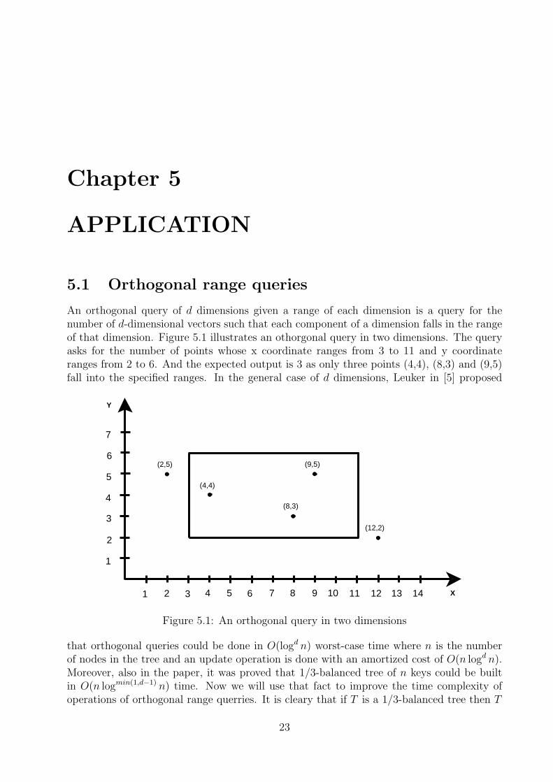
An orthogonal query of d dimensions given a range of each dimension is a query for thenumber of d-dimensional vectors such that each component of a dimension falls in the rangeof that dimension. Figure 5.1 illustrates an othorgonal query in two dimensions. The queryasks for the number of points whose x coordinate ranges from 3 to 11 and y coordinateranges from 2 to 6. And the expected output is 3 as only three points (4,4), (8,3) and (9,5)fall into the specified ranges. In the general case of d dimensions, Leuker in [5] proposed
1 2 3 4 5 6 7 8 9 10 11 12 13 14
1
2
3
4
5
6
7
(4,4)
(9,5)
(8,3)
(2,5)
(12,2)
X
Y
Figure 5.1: An orthogonal query in two dimensions
that orthogonal queries could be done in O(logd n) worst-case time where n is the numberof nodes in the tree and an update operation is done with an amortized cost of O(n logd n).Moreover, also in the paper, it was proved that 1/3-balanced tree of n keys could be builtin O(n logmin(1,d−1) n) time. Now we will use that fact to improve the time complexity ofoperations of orthogonal range querries. It is cleary that if T is a 1/3-balanced tree then T
23

is 2/3-weight-balanced. So in order to apply Generalized Theorem 4.5.1, we will need to findout what are function F , αbalanced, αtrigger. Due to the fact that 1/3-balanced tree of n keys
could be built in O(n logmin(1,d−1) n) time, we could determine that F (n) = logmin(1,d−1) n,αbalanced = 1/2 and αtrigger = 2/3. Then the following theorem follows from GeneralizedTheorem 4.5.1:
Theorem 5.1.1. A relaxed Scapegoat tree can handle a sequence of n Insert and m Search orDelete operations, beginning with an empty tree, with an amortized cost O(F (n) log1/αtrigger
n)per Insert or Delete and O(log1/αtrigger
k) worst-case time per Search, where k is the size ofthe tree the Search is performed on.
24

Chapter 6
CONCLUSIONS AND FUTURE
WORK
6.1 Conclusions
As shown in this report, a Scapegoat tree T is always loosely α-height-balanced after anyupdate operation. Such loosely α-height balance is due to rebuilding operation taken placeafter detecting some Scapegoat node, which is a sign of α-height unbalance and α-weightunbalance. But the rebuilding operation is shown to happen after enough update operationsto pay for cost of rebuilding subtree rooted at the Scapegoat node which is linear in thesize. Therefore, a Scapegoat tree T could handle any Search operation in worse-case com-plexity O(log(T.size)) and the amortized cost of any update operation is O(log(T.size)) time.
The Demo for this project is implemented successfully. Even though any update op-eration in the implementation is done in linear time in term of the size and that’s becauseall the nodes shown in UI needs to be redrawn after the operation. So the coordinates of allthe nodes need to be recomputed and all of them need to be redrawn. Aside from the UI,the Search, Insert, Delete operations that are implemented in the Scapegoat tree class trulyfollow the complexity of theoretical part. Through the implementation of and experimentswith the Demo, I have found out some helpful cases, for example, some Scapegoat treeafter some number of Insert and Delete operations is loosely α-height-balanced but notα-height-balanced. The case helps me to understand thoroughly the idea of Scapegoat treesto prove theorems and explain it in this report.
6.2 Future Work
There could be many improvements to the current project. First, I could investigate howScapegoat tree techniques could apply for quad trees in the original paper [3] or even in otherapplications not mentioned in the paper as well. Another improvement could come from theperformance of the Demo. Another method of drawing nodes could be explored so that whenrebuilding the subtree rooted at Scapegoat is taken place, the whole tree does not need to be
25

redrawn or just the rebuilt subtree needs to be redrawn. Finally, an alternative way to findthe Scapegoat node might be investigated. Finding Scapegoat node in the implementationof this project is done in the time of linear in the size of the subtree rooted at Scapegoat.The alternative way might reduce that kind of complexity into the logarithmic time in thesize of the whole tree because the search for a place to insert might give us some informationto detect the Scapegoat node.
26

REFERENCES
[1] R. Bayer. Symmetric binary b-trees: Data structure and maintenance algorithms. ActaInformatica, 1:290–306, 1972.
[2] Thomas H. Cormen. Introduction to Algorithms. The MIT Press, second edition edition,2001.
[3] Igal Galperin and Ronald L. Rivest. Scapegoat trees. In Proceedings of the fourth annualACM-SIAM Symposium on Discrete algorithms, pages 165 – 174. Society for Industrialand Applied Mathematics Philadelphia, PA, USA, 1993.
[4] Leo J. Guibas and Robert Sedgewick. A diochromatic framework for balanced trees. InProceedings of the 19th Annual Symposium on Foundations of Computer Sciences, pages28–34. IEEE Computer Soceity, 1978.
[5] George S. Leuker. A data structure for orthogonal range queries. In In Proceedings ofthe 19th Annual Symposium on Foundations of Computer Science, pages 28– 34. IEEEComputer Society, 1978.
[6] I. Nievergelt and E. M. Reinfold. Binary search trees of bounded balance. SIAM Journalon Computing, 2:33–43, 1973.
27

Appendix A
HOW TO USE THE DEMO
A.1 How to run
The Demo is already compiled and put in the folder Demo in the enclosed CD. It was writtenand compiled in Java version 1.5.0 06. To run the Demo, do the following steps if you don’thave any IDE to open those java files:
• Enter Command Prompt mode in Windows or Terminal mode in Linux
• Change the current folder to Demo on the CD
• Simply enter command java ScapegoatTreeDemo
A.2 How to do Search, Insert, and Delete
Important notice: For the purpose of demo, all input keys should be positive
integers.
Now when you would like to search, insert, or delete a node, just enter the key of anode in the text box below the text box of α then press the corresponding buttons. If yousearch for or delete a node , for example, node 9 that is not in the tree, you will get theerror message “Node 9 does not exist” in the output text box like in Figure A.1.
While inserting a node already in the tree for example node 5, you will get the error message“Node 5 already exists” like in Figure A.2.If inserting a node results in rebuilding a subtree rooted at Scapegoat node , for example,node 8, you will get the prompting messages: “Scapegoat Node 8 is detected” and “The treerooted at Scapegoat is going to be rebuilt.” like in Figure A.3 and A.4.
A.3 How to reset tree with a new α
Sometimes, if you would like to experience a new value of α, just simply enter a new valuein the input text box of alpha and press Reset button. The current tree is deleted and you
28

Figure A.1: Removing a node that does not exist in a Scapegoat tree
Figure A.2: Inserting a node that already exists in a Scapegoat tree
29

Figure A.3: A Scapegoat tree before inserting a node that leads to rebuilding
Figure A.4: A Scapegoat tree after inserting a node with rebuidling subtree rooted at Scape-goat
30

will need to build the new tree from scratch like in Figure A.5
Figure A.5: After resetting the new value of α
31

Appendix B
LIST OF FIGURES AND TABLES
32
List of Figures
1.1 A binary search tree with α = 0.6 . . . . . . . . . . . . . . . . . . . . . . . . 41.2 A weight-unbalanced binary search tree with α = 0.6 . . . . . . . . . . . . . 51.3 A height-unbalanced binary search tree with α = 0.55 . . . . . . . . . . . . . 61.4 An incomplete binary search tree . . . . . . . . . . . . . . . . . . . . . . . . 7
2.1 A sample Scapegoat tree from the Demo . . . . . . . . . . . . . . . . . . . . 82.2 A Scapegoat tree before insertion . . . . . . . . . . . . . . . . . . . . . . . . 102.3 A Scapegoat tree after insertion . . . . . . . . . . . . . . . . . . . . . . . . . 102.4 A Scapegoat tree before series of deletion . . . . . . . . . . . . . . . . . . . . 122.5 A Scapegoat tree after series of deletions . . . . . . . . . . . . . . . . . . . . 122.6 A Scapegoat tree after series of deletions and rebuilding . . . . . . . . . . . . 12
5.1 An orthogonal query in two dimensions . . . . . . . . . . . . . . . . . . . . . 23
A.1 Removing a node that does not exist in a Scapegoat tree . . . . . . . . . . . 29A.2 Inserting a node that already exists in a Scapegoat tree . . . . . . . . . . . . 29A.3 A Scapegoat tree before inserting a node that leads to rebuilding . . . . . . . 30A.4 A Scapegoat tree after inserting a node with rebuidling subtree rooted at
Scapegoat . . . . . . . . . . . . . . . . . . . . . . . . . . . . . . . . . . . . . 30A.5 After resetting the new value of α . . . . . . . . . . . . . . . . . . . . . . . . 31
33

List of Tables
1 Examples of notations for a binary tree node 8 in Figure 1.1 . . . . . . . . . 52 Examples of notations for a binary search tree in Figure 1.1 . . . . . . . . . 5
34