Embed Size (px)
Citation preview
Castalia
A simulator for Wireless Sensor Networks
and Body Area Networks
Version 3.2
User‟s Manual
Athanassios Boulis
March 2011
NICTA

2

3
Contents
1 Introduction....................................................................................................................... 5
1.1 Why a new simulator? .............................................................................................. 6
2 Overview........................................................................................................................... 7
2.1 Structure ................................................................................................................... 7
3 Using Castalia ................................................................................................................. 10
3.1 Running the first simulation ................................................................................... 10
3.2 Understanding the configuration file ..................................................................... 14
3.3 Using the Castalia and CastaliaResults scripts ....................................................... 20
3.4 Using CastaliaPlot to create graphs........................................................................ 28
3.5 Advanced usage ..................................................................................................... 30
3.5.1 Manipulating the display of a results table ........................................................ 33
3.5.2 Multiple repetitions and confidence intervals .................................................... 35
3.5.3 Changing configurations at command line ........................................................ 39
3.6 Complex simulation examples ............................................................................... 40
3.6.1 Body Area Network simulation example........................................................... 40
3.6.2 Bridge Test simulation example ........................................................................ 49
4 Modeling in Castalia ....................................................................................................... 51
4.1 The Wireless Channel ............................................................................................ 51
4.1.1 Average path loss modeling ............................................................................... 52
4.1.2 Allowing for node mobility ............................................................................... 53
4.1.3 Temporal variation modeling ............................................................................ 55
4.1.4 Delivering signals to the Radio module ............................................................. 58
4.1.5 Choosing naive models ...................................................................................... 59
4.2 The Radio ............................................................................................................... 60
4.2.1 The Radio Parameters file ................................................................................. 60
4.2.2 Radio Module Parameters .................................................................................. 62
4.2.3 Reception and Interference calculation .............................................................. 64
4.2.4 Dynamically adjusting radio parameters ........................................................... 65
4.3 MAC ...................................................................................................................... 67
4.3.1 Tunable MAC .................................................................................................... 67
4.3.2 T-MAC and S-MAC .......................................................................................... 72
4.3.3 IEEE 802.15.4 MAC.......................................................................................... 75
4.3.4 Baseline BAN MAC .......................................................................................... 78

4
4.4 Routing ................................................................................................................... 80
4.5 The Physical Process .............................................................................................. 82
4.5.1 Customizable Physical Process .......................................................................... 82
4.5.2 Cars Physical Process ........................................................................................ 84
4.6 The Sensor Manager .............................................................................................. 85
4.7 The Mobility Manager ........................................................................................... 87
4.8 The Resource Manager .......................................................................................... 88
5 Creating your own Application, Routing, MAC, and Mobility Manager modules ........ 89
5.1 Collecting Output and Defining Timers ................................................................. 92
5.1.1 Collecting Output............................................................................................... 92
5.1.2 Defining and Using Timers ............................................................................... 93
5.2 Defining a new Application module ...................................................................... 95
5.2.1 The ThroughputTest application example ......................................................... 98
5.2.2 Defining your own application packets ............................................................. 98
5.3 Defining a new Routing module .......................................................................... 100
5.3.1 BypassRouting module .................................................................................... 102
5.4 Defining a new MAC module .............................................................................. 102
5.4.1 The TunableMAC module example ................................................................ 104
5.5 Defining a new Mobility manager module .......................................................... 105
6 Appendix: Full List of Modules and Parameters .......................................................... 107
6.1 List of Modules .................................................................................................... 107
6.2 List of Parameters ................................................................................................ 108
7 References..................................................................................................................... 120

5
1 Introduction
Castalia is a simulator for Wireless Sensor Networks (WSN), Body Area Networks
(BAN) and generally networks of low-power embedded devices. It is based on the OMNeT++
platform and can be used by researchers and developers who want to test their distributed
algorithms and/or protocols in realistic wireless channel and radio models, with a realistic
node behaviour especially relating to access of the radio. Castalia can also be used to evaluate
different platform characteristics for specific applications, since it is highly parametric, and
can simulate a wide range of platforms. The main features of Castalia are:
Advanced channel model based on empirically measured data.
o Model defines a map of path loss, not simply connections between nodes
o Complex model for temporal variation of path loss
o Fully supports mobility of the nodes
o Interference is handled as received signal strength, not as separate feature
Advanced radio model based on real radios for low-power communication.
o Probability of reception based on SINR, packet size, modulation type. PSK
FSK supported, custom modulation allowed by defining SNR-BER curve.
o Multiple TX power levels with individual node variations allowed
o States with different power consumption and delays switching between them
o Realistic modelling of RSSI and carrier sensing
Extended sensing modelling provisions
o Highly flexible physical process model.
o Sensing device noise, bias, and power consumption.
Node clock drift
MAC and routing protocols available.
Designed for adaptation and expansion.
Concerning the last bullet, Castalia was designed right from the beginning so that the
users can easily implement/import their algorithms and protocols into Castalia while making
use of the features the simulator is providing. Proper modularization and a configurable,
automated build procedure help towards this end. The modularity, reliability, and speed of
Castalia is partly enabled by OMNeT++, an excellent framework to build event-driven
simulators [OMNeT++ link].

6
What Castalia is not: Castalia is not sensor-platform specific. Castalia is meant to
provide a generic reliable and realistic framework for the first order validation of an algorithm
before moving to implementation on a specific sensor platform. Castalia is not useful if one
would like to test code compiled for a specific sensor node platform. For such usage there are
other simulators/emulators available (e.g., Avrora).
1.1 Why a new simulator?
There is a variety of simulators that WSN researchers are using to cover their needs.
Simulators that emulate a common processor found in sensor nodes (to test actual binary code
written for certain platforms), simulators written in C++ or Matlab to test some first order
property of an algorithm, or simulators used in traditional data networks modified in some
way to serve the WSN community. So why try to build a new one?
It all started from our own needs in a WSN project. We wanted to test some
communication patterns in simulation before moving in real systems. In order to do so we
wanted accurate enough radio/channel models so that the simulation results would become
meaningful and guide us in our search. We knew of the work by Zuniga et al. [1] that
explained empirically measured data from WSN platforms (more specifically packet
reception rate as a function of distance) by combining known wireless channel and radio
models. We found that all the available WSN simulators were falling short of the current
state of the art modelling done in sensor networks. Especially in communication where the
impact to the result can be significant [5], models remain simplistic or unsuitable for short
range low power communications despite the existence of proper models developed the last
couple of years. This was the major reason we decided to build our own simulator. We used
OMNeT++ as the base to build a reliable and fast event-driven simulator. Using OMNeT++
meant that we could just focus on the models and overall design and not on the event-driven
simulation engine. Shortly after, we have decided to "up the ante", capture realistic node
behaviour beyond the channel and build an open expandable and reliable simulator that has a
chance of becoming a de facto standard for certain WSN simulation needs. More specifically,
the need for early stage, platform-independent, algorithm/protocol validation. Since its initial
inception and creation, Castalia has moved to new territories: BAN is another exciting area
where realistic and reliable network-level simulators are needed. NICTA has a large scale
project in BAN, participating at the same time in the IEEE standards BAN task group. With
our expertise in physical layer design, measurements and modeling, we have set out to make
Castalia the most realistic BAN network simulator, by modelling the temporal variations and
average path losses based on real on-body measurements.

7
2 Overview
Castalia is using OMNeT++ as its base so it is suggested that you have a fair
understanding of the basic concepts of OMNeT although this is not required, especially if you
want to use Castalia in a basic way (i.e., without building your own protocols/applications)
OMNeT‟s basic concepts are modules and messages. A simple module is the basic unit
of execution. It accepts messages from other modules or itself, and according to the message,
it executes a piece of code. The code can keep state that is altered when messages are
received and can send (or schedule) new messages. There are also composite modules. A
composite module is just a construction of simple and/or other composite modules.
2.1 Structure
Castalia‟s basic module structure is shown in the diagram below.
Figure 1: The modules and their connections in Castalia
Notice that the nodes do not connect to each other directly but through the wireless
channel module(s). The arrows signify message passing from one module to another. When a
node has a packet to send this goes to the wireless channel which then decides which nodes
should receive the packet. The nodes are also linked through the physical processes that they
monitor. For every physical process there is one module which holds the “truth” on the
quantity the physical process is representing. The nodes sample the physical process in space
and time (by sending a message to the corresponding module) to get their sensor readings.
Node 2 …
Physical process 1
Wireless Channel
Node 1 Node N

8
There can be multiple physical processes, representing the multiple sensing devices (multiple
sensing modalities) that a node has.
The node module is a composite one. Figure 2 shows the internal structure of the node
composite module. The solid arrows signify message passing and the dashed arrows signify
simple function calling. For instance, most of the modules call a function of the resource
manager to signal that energy has been consumed. The Application module is the one that the
user will most commonly change, usually by creating a new module to implement a. new
algorithm. The communications MAC and Routing modules, as well as the Mobility Manager
module, are also good candidates for change by the user, again usually by creating a new
module to implement a new protocol or mobility pattern. Castalia offers support for building
your own protocols, or applications by defining appropriate abstract classes (more on this
topic in Chapter 5). All existing modules are highly tuneable by many parameters.
Figure 2: The node composite module
This structure depicted in the figures above and described in this chapter is
implemented in Castalia with the use of the OMNeT++ NED language. With this language
we can easily define modules, i.e., define a module name, module parameters, and module
interface (gates in and gates out) and possible submodule structure (if this is a composite
module). Files with the suffix “.ned” contain NED language code. The Castalia structure is
also reflected in the hierarchy of directories in the source code. Every module corresponds to
a directory which always contains a .ned file that defines the module. If the module is
Radio
MAC
Application
Radio
Sensors Manager Resource Manager
(Battery, CPU state,
Memory)
to/from Wireless Channel
to/from Physical Process C
om
munic
atio
ns
com
posi
te m
odule
Routing
Mobility Manager
location
Any module
(read only)
to wireless channel
9
composite then there are subdirectories to define the submodules. If it is a simple module then
there is C++ code (.cc, .h files) to define its behaviour. This complete hierarchy of .ned files
defines the overall structure of the Castalia simulator. Normally the user will not alter these
files. Nevertheless, these files are dynamically loaded and processed (using a feature of
OMNeT) so that any change does not require the recompilation of Castalia (unless of course
new simple modules with new functionality appear).
In the rest of this document we will use these formatting conventions:
Commands given at the shell and output produced by them:
current_path$ commandline
Outputlines
Outputlines
Portions of configuration files (usually named omnetpp.ini):
Parameter1 = 1
Parameter2 = 2
C++ code or NED scripting code:
Code
Paths, file names, and parameter names will be written in Courier fonts. Castalia/ is
assumed to be the top-most level directory where all the Castalia files are installed.

10
3 Using Castalia
We assume here that you successfully installed both OMNeT and Castalia. Refer to the
Installation Guide for details and troubleshooting. Since the release of Castalia 3.0, handling
of input and output has changed considerably. We advise you to read this section even if you
had previous experiences with Castalia 2.3b or earlier releases. Since Castalia 3.0, we have
two scripts to help with running simulations and interpreting the results. They are called
Castalia and CastaliaResults respectively. Since release 3.1 we also have
CastaliaPlot to help you create graphs. They all reside in Castalia/bin/1. The
executable of the simulator is called CastaliaBin resides in Castalia/ but you will
not need to invoke it directly.
3.1 Running the first simulation
It‟s time to dive in and run our first simulation. Go to the directory
Castalia/Simulations/radioTest. It should include one file: omnetpp.ini.
This is a configuration file that defines our simulation scenario(s). Let us run the input script
with no arguments and see what we get:
~/Castalia/Simulations/radioTest$ ../../bin/Castalia
List of available input files and configurations:
* omnetpp.ini
General
InterferenceTest1
InterferenceTest2
CSinterruptTest
varyInterferenceModel
Executed with no arguments, the script searches the current directory for valid configuration
files. If it finds a file, it then parses it and prints the name of the configurations contained in it
(more about configurations shortly). In our case it found just one file with five configurations.
1 It is suggested that you add Castalia/bin/ in your PATH env variable. In the command line examples
we give in this manual, we assume that Castalia/bin is in the path. If you are using bash you simply do
$ export PATH=$PATH:~/Castalia/bin
(assuming Castalia‟s dir is named “Castalia” and it is installed under your home dir)
Also do not forget to add this export statement in your .bash_profile file

11
To see how we can use the Castalia input script to do something more exciting, ask for
help. Run it with -h as argument.
~/Castalia/Simulations/radioTest$ ../../bin/Castalia -h
Usage: Castalia [options]
Options:
-h, --help show this help message and exit
-c CONFIG, --config=CONFIG
A list of configuration names to use, comma
separated configurations will be joined
together, configurations listed in brackets
will be interleaved
-i FILE, --input=FILE
Select input configuration file, default is
omnetpp.ini
-d, --debug Debug mode, will display results from each
CastaliaBin execution
-o FILE, --output=FILE
Select output file for writing results,
generated from current date by default
-r N, --repeat=N Number of repetitions for each unique
scenario
We see that we can instruct the Castalia script to use a specific file with the -i switch
(although we do not need to in our case, omnettpp.ini is the default) and use the -c switch to
choose a configuration within this file. For the moment do not mind the help-text mentioning
that a list of configuration can be given, and just run it with one configuration. Let‟s use
General, which is always present in an omnetpp.ini file and is considered the default
configuration.
~/Castalia/Simulations/radioTest$ ../../bin/Castalia -c General
Running configuration 1/1
You‟ve just run your first simulation! Let‟s see what‟s new in our directory.
~/Castalia/Simulations/radioTest$ ls
100806-222319.txt Castalia-Trace.txt omnetpp.ini
There are 2 new files created: 100806-222319.txt is Castalia‟s standard output file and
its name is in the form YYMMDD-HHMMSS.txt. You can freely rename this file if you wish.

12
You can also open it to read it (it is human readable) but it is not supposed to be viewed this
way. Normally you will process this file with CastaliaResults. We will see how to do
this in section 3.3. The other file produced is a trace file named Castalia-Trace.txt. It
contains a trace of all events that you requested to be recorded by “turning on” some
parameters in the omnetpp.ini file. By default all tracing is turned off, but for this simulation
example we wanted to activate just the tracing from the application module of node 0. Open
the file and have a look.
~/Castalia/Simulations/radioTest$ less Castalia-Trace.txt
0.027540267327 SN.node[0].Application Not sending packets
3.868527053713 SN.node[0].Application Received packet #18 from node 1
4.068529304763 SN.node[0].Application Received packet #19 from node 1
4.268531555813 SN.node[0].Application Received packet #20 from node 1
4.468533806863 SN.node[0].Application Received packet #21 from node 1
4.668536057913 SN.node[0].Application Received packet #22 from node 1
…
Each line is a trace event. The first item in the line is the simulation time that the event
happened. Second item is the full name of the module that produced this trace line. In the
example above all lines are produced by the Application module of node 0. Finally, the last
item is the trace message itself. In the example above most messages notify us of packet
received by node 1, also printing the packet‟s serial number.
But what is this simulation supposed to do?
We created the radioTest simulation scenarios so users can see the results of realistic
modeling and also see some of Castalia‟s features in action. The first scenario (the General
configuration we just run) tests reception, as a receiver (node 0) moves through the area of
two transmitters (nodes 1 and 2). The transmitters are placed far enough so there is no
interference between them. The receiver moves in a straight line back and forth and when it
is close to each of the two transmitters it should receive their packets. For this simulation we
have turned off shadowing effects so that the successful-reception-distance is identical for the
two transmitters (still there are random effects in the radio reception, so the numbers of
received packets by the two transmitters are not identical). The InterferenceTest1 and
InterferenceTest2 scenarios have the receiver static and one of the transmitters moving. The
idea there is to show the effect of interference with the use of mobility. In InterferenceTest1
the interfering node passes through the middle of the distance between node 1 and 0, and thus

13
just causes collisions. In InterferenceTest2 though it passes very close to the receiver
(compared to the other transmitter) and thus even though initially it creates collisions, when
sufficiently close, its SINR is high enough for its packets to be received (despite interference
from the transmissions of static node 1). Figure 3 illustrates these interactions.
Figure 3: The General, InterferenceTest1, and InterferenceTest2 configurations
Run the other two simulation scenarios and look at the resulting Castalia-Trace.txt files
(delete the old trace files if you do not want the new traces appended in the old file).
~/Castalia/Simulations/radioTest$ rm Castalia-Trace.txt
~/Castalia/Simulations/radioTest$ Castalia -c InterferenceTest1
Running configuration 1/1
Are the traces as expected? You should be able to see the patterns of reception and
breaking of reception as depicted in figure 3.
Let‟s us look more deeply into the omnetpp.ini file.
Node 0
Node 2
Node 1 Node 0
Node 1
Node 2 Node 2
Node 1
Node 0
Receiver node
Transmitter node
Receive pcks from node 1
Receive pcks from node 2
collision

14
3.2 Understanding the configuration file
As described in Chapter 2, Castalia has a modular structure with many interconnecting
modules. Each one of the modules has one or more parameters that affect its behavior. An
NED file (file with extension .ned in the Castalia source code) defines the basic structure of a
module by defining its input/output gates and its parameters. In the NED file we can also
define default values for the parameters. A configuration file (usually named omnetpp.ini and
residing in the Simulations dir tree) assigns values to parameters, or just reassigns them to a
different value from their default one. This way we can build a great variety of simulation
scenarios. Open the file Simulations/radioTest/omnetpp.ini
Note that any string after a # character is a comment. The configuration file starts with
the General section. Every OMNeT configuration file has a General section. There you define
the basic scenario that this file describes. Parameters such as the simulation time and number
of nodes do not have any default values and must be defined in this section. Below are the
first few lines from the radioTest/omnetpp.ini file (comments removed)
[General]
include ../Parameters/Castalia.ini
sim-time-limit = 100s
SN.field_x = 200 # meters
SN.field_y = 200 # meters
SN.numNodes = 3
The first line in the General section is an include command. As the name suggests, the
command includes the contents of the file it gets as an argument. In the particular example we
include a file we named Castalia.ini and it contains some basic parameter assignments2 that
every Castalia simulation needs. So when you create a Castalia configuration file, always
include Castalia.ini in it.
Then we define the simulation time (here assigned to 100 secs). This is the only generic
OMNeT parameter we assign in a Castalia configuration file. We can see that all other
parameter start their name with SN. SN is the topmost composite module (or “network” as
OMNeT calls it). The name SN stands for Sensor Network. There are a few parameters that
2 Castalia.ini assigns some parameters affecting general OMNeT execution, as well as parameters that
map the different Random Number Generators (RNGs) to modules.

15
the network takes such as the field size, the number of nodes, and the deployment type. The
field size is given by 3 real numbers, each for axes x,y,z. One can define only 2 of the axes if
desired (the third one will take the value 0 by default). Number of nodes is given by an
integer. The parameter SN.deployment is a string that describes where the nodes are
placed on the field. If left undefined (as in our example above) then the location of the nodes
is determined by the xCoor, yCoor, zCoor parameters of each node. These are usually
manually assigned in the omnetpp.ini file. When defined, SN.deployment can be one of
the following types:
“uniform” nodes are placed in the field using a random uniform distribution
“NxM” N and M are integer numbers. Nodes placed in a grid of N nodes by M nodes
“NxMxK” same as above but for 3 dimensions
“randomized_NxM” a grid deployment with randomness in the position of the nodes.
If Gx and Gy is the grid spacing in axes x and y, and (Xi, Yi) are
the grid position of node i then the randomized grid position is
(Xi+Rx, Yi+Ry) where Rx and Ry are numbers uniformly drawn
from [(-1/3)Gx…(1/3)Gx ] and [(-1/3)Gy…(1/3)Gy ]
“randomized_NxMxK” same as above but for 3 dimensions
“center” node put in the centre of the field
We can even define mixed deployments by using this string format:
[N1..N2]->type;[N2..N3]->type;… where Nx are node IDs, and types is one of the options
given above
After we set these top level parameters, we go into setting module parameters. When
setting a module parameter, the full name of the module is given revealing the module
hierarchy structure. Here is an example from our configuration file, setting some parameters
of the wireless channel.
# important wireless channel switch to allow mobility
SN.wirelessChannel.onlyStaticNodes = false
SN.wirelessChannel.sigma = 0
SN.wirelessChannel.bidirectionalSigma = 0
We will explain the meaning and use of all parameters in Chapter 4 (Modeling in
Castalia). In this section we present some basic concepts and syntax rules of Castalia
configuration files.

16
For instance, how do we set radio parameters? Remember that the radio is part of the
Communication composite module of every node. So there are as many Radio modules as
there are nodes. How do we set all of them easily? Here‟s how:
SN.node[*].Communication.Radio.RadioParametersFile =
"../Parameters/Radio/CC2420.txt"
SN.node[*].Communication.Radio.TxOutputPower = "-5dBm"
These two lines set 2 parameters of the Radio module. The RadioParametersFile is a
specially formatted file defining the basic operational properties of a radio (more on Chapter
4). The second parameter, TxOutputPower sets the power that the radio transmits its packets.
Notice how we access all the radio modules in all the nodes with the use of [*].
The sensor network compound module (SN) contains many Node sub-modules. These
are addressed in the form of an array. For instance, here‟s how to set the parameter xCoor
(the x coordinate of the location of a node) of the node with ID=9:
SN.node[9].xCoor = 10.5
However, most of the time we need to massively assign values for all the nodes of the
sensor network. This is possible by using wildcards like:
[*] all indexes
[3..5] indexes 3,4,5
[..4] indexes 0, 1, 2, 3, 4
[5..] indexes 5 till the last one
Reading on in our example omnetpp.ini file we see that parameters relating to the
maximum allowed packet size are set in all communication layers:
SN.node[*].Communication.Routing.maxNetFrameSize = 2500
SN.node[*].Communication.MAC.maxMACFrameSize = 2500
SN.node[*].Communication.Radio.maxPhyFrameSize = 2500
We have already set the kind of radio we want to use, by setting RadioParametersFile.
How do we instruct Castalia which MAC protocol and which Routing protocol to use? This is
achieved by two Communication module parameters
SN.node[*].Communication.MACProtocolName
SN.node[*].Communication.RoutingProtocolName
These are set by default to "BypassMAC" and "BypassRouting". These are module
names that in essence implement no MAC functionality and no Routing functionality. For the
radioTest simulation we did not need any MAC or Routing so we left these parameters

17
assigned to their default value (i.e., they are not mentioned in the omnetpp.ini file). If you
want to see the default values for any parameter just go to the .ned file that describes that
module. For the parameters mentioned above you can look in:
src/node/communication/CommunicationModule.ned
If you look at the BANtest/omnetpp.ini you will see MACProtocolName being assigned
SN.node[*].Communication.MACProtocolName = "BaselineBANMac"
The important thing to note here is that by assigning a name to this parameter we are
also choosing a specific module for our MAC. So by altering these parameters we can
dynamically control the composition of modules in our simulation3. The consequence of this
feature is that depending on the module you choose, the parameters available to you are also
changing since different MAC modules support different parameters. There are four kinds of
modules that are dynamically selected in a Castalia configuration file. We have already seen
the 2 kinds: MAC and Routing modules. The other 2 are Application modules and
MobilityManager modules.
Here is how we set our radioTest simulation to use the Application module we want:
SN.node[*].ApplicationName = "ThroughputTest"
SN.node[*].Application.packet_rate = 5
SN.node[*].Application.constantDataPayload = 2000
# application's trace info for node 0 (receiving node)
# is turned on, to show some interesting patterns
SN.node[0].Application.collectTraceInfo = true
By setting the ApplicationName we also choose the application module.
ThroughputTest application has all nodes sending traffic to a sink node. We can easily
modify the packet rate and the packet size as you can notice. The sink node is by default node
0 and we have not changed this here. Also notice how the last line shown above, activates the
collecting of traces for the Application module of node 0. This is why the Castalia-
Trace.txt files we examined in section 3.1 were created and this is why they only
contained events from the application module of node 0. All Castalia modules have a
collectTraceInfo parameter. By default, collection of traces is deactivated (parameter
set to false).
3 This is achieved thanks to OMNeT‟s dynamic module loading capability and also its ability to define
parametric module names in .ned files.

18
Then follows a section where we set the starting locations for our 3 nodes manually
(remember that we left SN.deployment to its default value: “custom”). We write “starting
locations” because the nodes can be mobile. Indeed, we see that node 0 is using
LineMobilityManager as the mobility manager module. The other two nodes have the
default mobility manager: NoMobilityManager, which is used to describe static nodes.
SN.node[0].xCoor = 0
SN.node[0].yCoor = 0
SN.node[1].xCoor = 50
SN.node[1].yCoor = 50
SN.node[2].xCoor = 150
SN.node[2].yCoor = 150
SN.node[0].MobilityManagerName = "LineMobilityManager"
SN.node[0].MobilityManager.updateInterval = 100
SN.node[0].MobilityManager.xCoorDestination = 200
SN.node[0].MobilityManager.yCoorDestination = 200
SN.node[0].MobilityManager.speed = 15
The LineMobilityManager module moves the node in a straight line segment
(back and forth). The straight line segment is defined by the starting location of a node and
the destination location given by the xCoorDestination, yCoorDestination parameters of the
mobility module. We also define the speed and the update interval that the wireless channel
module will be updated of the node‟s current position.
After these lines we see a new section: a new configuration.
[Config InterferenceTest1]
SN.node[0].MobilityManagerName = "NoMobilityManager"
SN.node[1].MobilityManagerName = "NoMobilityManager"
SN.node[2].MobilityManagerName = "LineMobilityManager"
SN.node[0].xCoor = 10
SN.node[0].yCoor = 50
SN.node[1].xCoor = 0
SN.node[1].yCoor = 50
SN.node[2].xCoor = 5
SN.node[2].yCoor = 0
19
SN.node[2].MobilityManager.updateInterval = 100
SN.node[2].MobilityManager.xCoorDestination = 5
SN.node[2].MobilityManager.yCoorDestination = 100
SN.node[2].MobilityManager.speed = 5
In this configuration, node 2 is the mobile one, instead of node 0, and nodes are much
closer to each other (so that we can simulate interesting interference behaviour).
Yet another configuration section follows with slightly different node locations, which
we do not show here. Instead we draw your attention at the end of the file, where a very short
configuration section resides. Here it is:
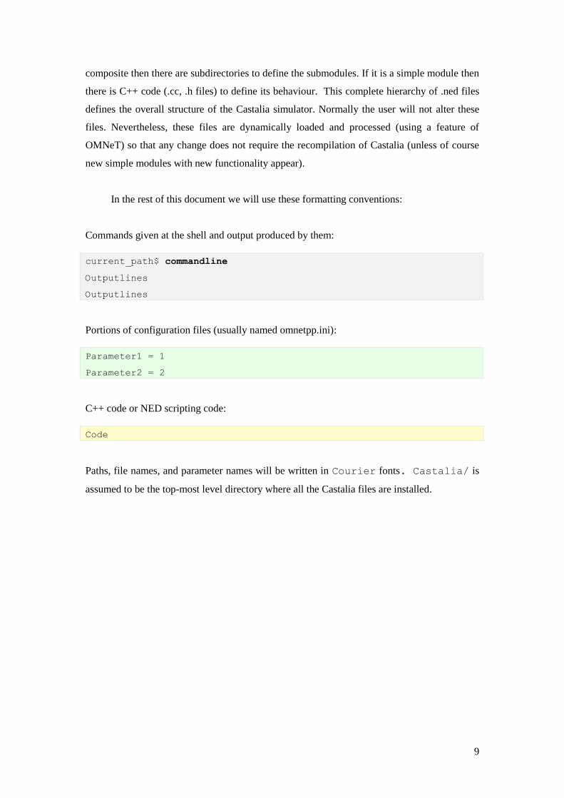
[Config varyInterferenceModel]
SN.node[*].Communication.Radio.collisionModel = ${InterfModel=0,1,2}
Notice how we do not assign just one value to the parameter but a series of values. This
is a feature of OMNeT 4.0 and later versions. You can look at the OMNeT manual for a
complete list of the ways you can assign parameters, but the essence of this multiple-value
assignment is that simulation will run many times, each time assigning one of the values. So
given the example above we will run the simulation 3 times. The name “InterfModel” in the
curly braces will just be used as a label in the output produced and helps us parse the output
more easily.
If you have more than one parameter that takes multiple values, then all combinations
will be run. In the example below we have 2 parameters taking 3 values each, which means 9
possible parameter combinations, thus 9 simulation runs.
SN.node[1].Communication.Radio.TxOutputPower = ${TxPower="-5dBm", "-10dBm", "-15dBm"}
SN.node[0].Communication.Radio.CCAthreshold = ${CCAthreshold=-95, -90, -85}
You can even do more complicated things such as putting constraints, so that not all
possible combinations are executed. Here‟s an example from BANtest/omnetpp.ini:
SN.node[*].Communication.MAC.scheduledAccessLength = ${schedSlots=6,5,4,3}
SN.node[*].Communication.MAC.RAP1Length = ${RAPslots=2,7,12,17}
constraint = $schedSlots * 5 + $RAPslots == 32
The example above will only execute 4 combinations: (6,2), (5,7), (4,12), (3,17).

20
3.3 Using the Castalia and CastaliaResults scripts
OMNeT allows you to choose just one of the configurations defined in a configuration
file. That is, if you use the simulator binary directly (i.e. CastaliaBin) you can choose an
input configuration file and one configuration. When choosing a configuration the parameters
from the General section are used and set, and if the configuration redefines them, then their
value is overwritten. Although this feature is an improvement over older versions, its
usefulness is limited. Notice for example, the configuration on varying the collision model we
examined earlier. If we choose it using OMNeT‟s standard feature it will only be applied in
the General section scenario. If we would like the same effect in the Interference scenarios
then we would have to explicitly include that line in each configuration. If we also wanted to
vary the Tx power but not vary the collision model, then we would have to explicitly write
another set of configurations. The problem is that you cannot easily combine configurations.
You have to explicitly write the combinations. Furthermore, you cannot easily execute more
than one configuration at a time. We can overcome these restrictions by using the Castalia
script.
With the Castalia script we can easily give a list of configurations to be combined.
For example, we can write “Castalia –c InterferenceTest1,varyInterferenceModel” or
“Castalia –c InterferenceTest2,varyInterferenceModel” no need to create the combination
explicitly in the omnetpp.ini file. Moreover we have the ability to define more than one
configuration to be executed by listing different configurations in braces. Castalia –c [A,B]
will execute the simulation with configuration A and then another simulation with
configuration B.
Castalia –c [A,B]C,D[E,F] will execute 4 combined configurations:
A,C,D,E this is a combination (or concatenation) of the 4 simple configs listed
B,C,D,E
A,C,D,F
B,C,D,F
If you try to combine two or more configurations that have at least one overlapping
parameter (i.e. same parameter is defined in two or more configurations) then you will get an
error message from the script. For example if you tried:
radioTest$ Castalia -c InterferenceTest1,InterferenceTest2
ERROR: conflicting values for parameter 'SN.node[2].xCoor' in base
configurations: '5' and '22'
Let us use the power of the Castalia script to run a useful simulation:

21
$ Castalia -c [InterferenceTest1,InterferenceTest2]varyInterferenceModel
Running configuration 1/2
Running configuration 2/2
A new output file was created (in our system 100809-004640.txt) and Castalia-
Trace.txt got appended with new traces. How would you check the results? You could
open the output file or the trace, but there is a lot of text to parse and understand. Remember
that for each of the configurations we have 3 collision models tried, so in total we had 6
simulations run. We need a way to process and summarize the results. This is what the script
CastaliaResults is for. Let‟s run it with no arguments to see what it gives us:
~/Castalia/Simulations/radioTest$ CastaliaResults
Castalia output files in current directory:
+-------------------+---------------------------------+------------------+
| | Configuration | Date |
+-------------------+---------------------------------+------------------+
| 100807-160236.txt | General (1) | 2010-08-07 16:02 |
| 100808-014651.txt | InterferenceTest1 (1) | 2010-08-08 01:46 |
| 100809-004640.txt | [InterferenceTest1,Interference | 2010-08-09 00:46 |
| | Test2]varyInterferenceModel (1)| |
+-------------------+---------------------------------+------------------+
It gives us a list of valid Castalia output files (also called result files) with information
about the configuration that created them and the date they were created. The number in the
parentheses (1) denotes the repetitions (with different seeds) each configuration was executed.
You can use the –h option to get help on the arguments the script can take. Let‟s run the script
giving it one of the results file as input (use the –i switch)
radioTest$ CastaliaResults -i 100809-004640.txt
+---------------------+----------------------------------+------------+
| Module | Output | Dimensions |
+---------------------+----------------------------------+------------+
| Application | Application level latency, in ms | 1x2(11) |
| | Packets received per node | 1x2 |
| Communication.Radio | RX pkt breakdown | 3x1(6) |
| | TXed pkts | 2x1 |
| ResourceManager | Consumed Energy | 3x1 |
+---------------------+----------------------------------+------------+
NOTE: select from the available outputs using the -s option

22
CastaliaResults parses the file and finds out what output is recorded by the
different modules. Application for example produces two kinds of output relating to packet
latency and packets received. Each output has its dimensions NxM.
N is the number of modules that produced this output. Modules that are instantiated
only once (e.g., the wirelessChannel) will always have N=1. Modules that are instantiated n
times (e.g., the node and all of its submodules) can have N equal up to n. In the example
above, even though there are 3 Application modules (recall that radioTest simulations
instantiate 3 nodes), only one of them is producing output. This is the Application module of
node 0, since this is the only one receiving packets.
M, is the number of different indices, an output from a single module has. When
defining an output, it is possible to give it an index parameter. Usually this is used to
differentiate output relating to different nodes. For example the “Packets received per node”
output has an index specifying the sender of the packet. This way we can keep track of how
many packets did a node receive from the different senders. If an output does not have an
index (e.g., the consumed energy output of a node) then M=1.
Finally, if an output from a single module and for a single index is not scalar, then we
write its multiplicity in parentheses. For example, the latency output is a histogram with 11
time buckets. As another example, the Radio received packet breakdown has 6 different types
of packets. The types are naming the different conditions the packets failed or succeeded.
The note at the end of the output above urges us to use the -s switch („s‟ standing for
„show‟) to select among the possible outputs. You just give it a regular expression and it will
present the results from the output names that match the regular expression. Let‟s say we
want to see what the application packets results are:
radioTest$ CastaliaResults -i 100809-004640.txt -s packets
Application:Packets received per node
+-------------------+---------------+---------------+---------------+
| | InterfModel=0 | InterfModel=1 | InterfModel=2 |
+-------------------+---------------+---------------+---------------+
| InterferenceTest1 | 335.5 | 12 | 99.5 |
| InterferenceTest2 | 332.5 | 11.5 | 24.5 |
+-------------------+---------------+---------------+---------------+
We see the results for both interference tests for all 3 collision modes in a nice 2×3
matrix. The results in each cell are averages for all modules that produced this output and all
indices of the output. In our case it is the average received packets per node at node 0 (since
the app of node 0 is the only module that produces this output as we mentioned). The average
23
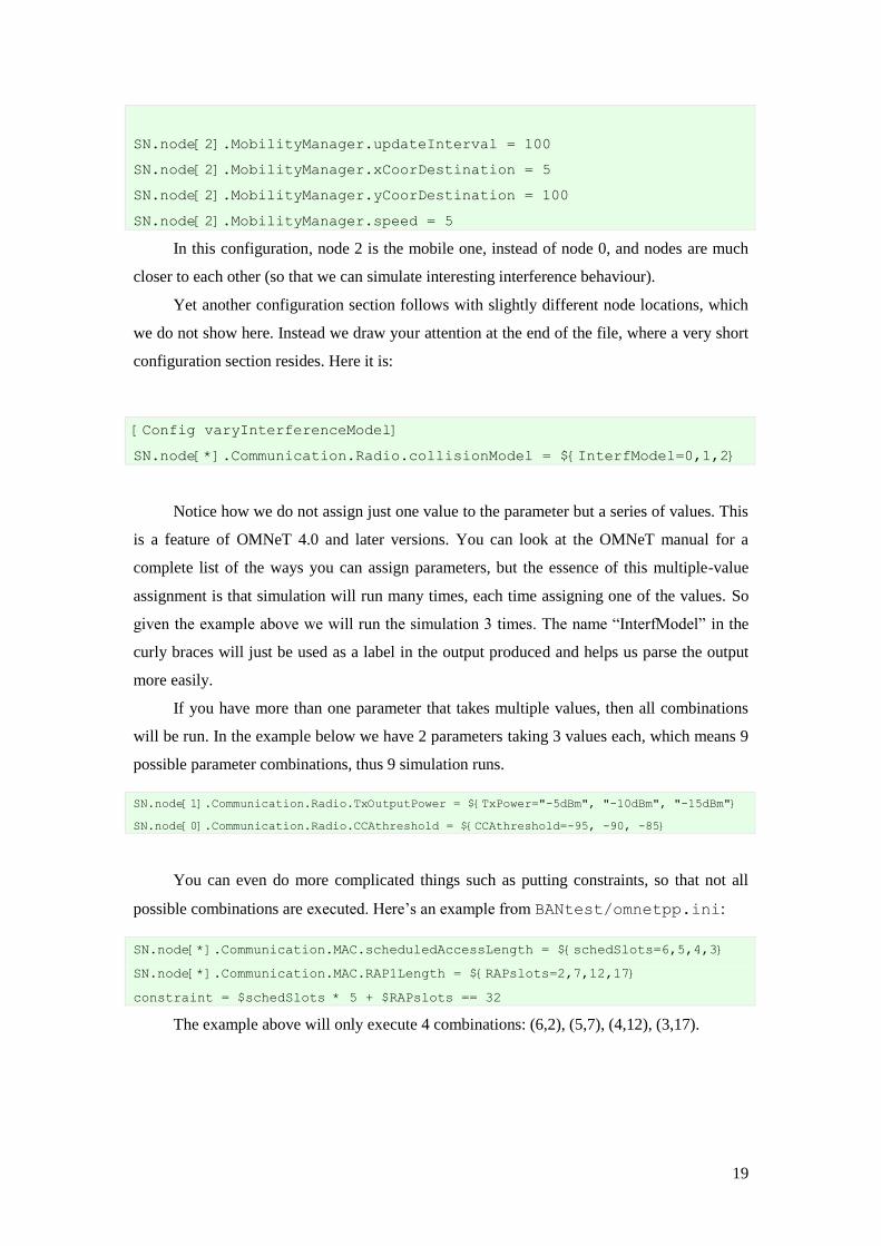
is calculated over 2 indices (sender node 1 and 2). Instead of the average we can see the sum
by using the switch --sum.
radioTest$ CastaliaResults -i 100809-004640.txt -s packets --sum
Application:Packets received per node
+-------------------+---------------+---------------+---------------+
| | InterfModel=0 | InterfModel=1 | InterfModel=2 |
+-------------------+---------------+---------------+---------------+
| InterferenceTest1 | 671 | 24 | 199 |
| InterferenceTest2 | 665 | 23 | 49 |
+-------------------+---------------+---------------+---------------+
This sum info is trivial in our case, since we know that we always have 2 indices so we
can just multiply the average results by 2, but in some cases the --sum switch can be very
useful. For example, when we do not know the number of elements that contribute to the
average, or the number is changing for different cells of the output table. Returning to our
specific example, the average (or sum) table gives us an understanding of the situation but it
would be more informative if we could see the results for the individual sender. We can do
this by using the -n switch („n‟ standing for „node‟). Let‟s try it:
radioTest$ CastaliaResults -i 100809-004640.txt -s packets -n
Application:Packets received per node
+---------------------------------+---------+---------+
| | Index=1 | Index=2 |
+---------------------------------+---------+---------+
| InterferenceTest1,InterfModel=0 | 499 | 172 |
| InterferenceTest1,InterfModel=1 | 24 | 0 |
| InterferenceTest1,InterfModel=2 | 199 | 0 |
| InterferenceTest2,InterfModel=0 | 494 | 171 |
| InterferenceTest2,InterfModel=1 | 23 | 0 |
| InterferenceTest2,InterfModel=2 | 25 | 24 |
+---------------------------------+---------+---------+
A new dimension called “index” was added to the results table. The table of results
became 6×2 and now the columns are labeled with an index which is the ID of the sender
node. Note that for a given row, the sum of the cells is equal to the contents of a cell from the
previous table (the table we got with --sum). But now we can see how this sum breaks down.
We see that when interference model = 0 is used (i.e., no collisions) then node 0 receives the
most packets from both node 1 and 2. Node 2 moves, so it is often outside the range of node
0. That‟s why fewer packets are received from it. There is some randomness at the Radio
module (packet reception probability is based on SNR) so the packets received from node 1
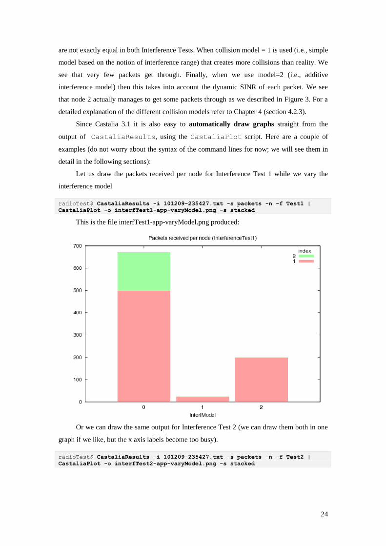
24
are not exactly equal in both Interference Tests. When collision model = 1 is used (i.e., simple
model based on the notion of interference range) that creates more collisions than reality. We
see that very few packets get through. Finally, when we use model=2 (i.e., additive
interference model) then this takes into account the dynamic SINR of each packet. We see
that node 2 actually manages to get some packets through as we described in Figure 3. For a
detailed explanation of the different collision models refer to Chapter 4 (section 4.2.3).
Since Castalia 3.1 it is also easy to automatically draw graphs straight from the
output of CastaliaResults, using the CastaliaPlot script. Here are a couple of
examples (do not worry about the syntax of the command lines for now; we will see them in
detail in the following sections):
Let us draw the packets received per node for Interference Test 1 while we vary the
interference model
radioTest$ CastaliaResults -i 101209-235427.txt -s packets -n -f Test1 |
CastaliaPlot -o interfTest1-app-varyModel.png -s stacked
This is the file interfTest1-app-varyModel.png produced:
Or we can draw the same output for Interference Test 2 (we can draw them both in one
graph if we like, but the x axis labels become too busy).
radioTest$ CastaliaResults -i 101209-235427.txt -s packets -n -f Test2 |
CastaliaPlot -o interfTest2-app-varyModel.png -s stacked

25
Or we can look at the output of a different module than the application. For instance we
can look at the breakdown of packets at the radio of node 0, for Interference Test 1 and for
different interference models.
radioTest$ CastaliaResults -i 101209-235427.txt -s RX -n -f Test1.*node=0 |
CastaliaPlot -o interfTest1-RadioBrdown-varyModel.png -s stacked --
colors=radioBrdown -l "outside width -7"

26
Let us now move to a different simulation scenario and a different application
altogether. The connectivity map application: This application is designed to produce a
connectivity map of the network by finding out the link quality between nodes. Each node is
programmed to transmit 100 packets at a unique timeslot, so that there are no collisions with
other nodes. A node –when not transmitting– constantly listens for incoming packets, and
when one is received, it increases the counter of the packets heard from the sender node. At
the end of the simulation the counters are written as application output using the sender node
as index. Go to Simulations/connectivityMap/ and inspect the omnetpp.ini file
The configuration file describes a grid of 3nodes×3nodes (9 nodes in total). The
General configuration has a wireless channel with no shadowing randomness and the radio is
using a low Tx power. Let‟s run it and inspect the results.
connectivityMap$ Castalia -c General
Running configuration 1/1
connectivityMap$ ls
100809-145319.txt omnetpp.ini
connectivityMap$ CastaliaResults -i 100809-145319.txt
+---------------------+------------------+------------+
| Module | Output | Dimensions |
+---------------------+------------------+------------+
| Application | Packets received | 9x9 |
| Communication.Radio | RX pkt breakdown | 9x1(3) |
| | TXed pkts | 9x1 |
| ResourceManager | Consumed Energy | 9x1 |
+---------------------+------------------+------------+
NOTE: select from the available outputs using the -s option
We see that the Application module output “Packets received” is 9×9. This means that
there are 9 modules reporting and for each module there are 9 indices (each corresponding to
other nodes + the self node). Simply printing the result of that output will give us the average
on these 9×9 (= 81) outputs. This will be the average link quality over all the links4.
connectivityMap$ CastaliaResults -i 100809-145319.txt -s packets
Application:Packets received
+--------+
4 It is the average of link quality for links that are not 0%, i.e. at least one packet was successfully
received.

27
| |
+--------+
| 88.225 |
+--------+
This in not such an interesting result, on its own. It would be much more interesting if
we could see the quality of individual links. How many packets out of the 100 did each link
(node A node B) was able to receive. We need to show individual outputs, not the average.
We already mentioned that if we want to expand an output to its dimensions we use the –n
switch. Let‟s try it.
connectivityMap$ CastaliaResults -i 100809-145319.txt -s packets -n
Application:Packets received
+--------+-------+-------+-------+-------+-------+-------+-------+-------+-------+
| |Node=0 |Node=1 |Node=2 |Node=3 |Node=4 |Node=5 |Node=6 |Node=7 |Node=8 |
+--------+-------+-------+-------+-------+-------+-------+-------+-------+-------+
|index=0 | 0 | 100 | 0 | 99 | 73 | 0 | 0 | 0 | 0 |
|index=1 | 100 | 0 | 100 | 70 | 100 | 72 | 0 | 0 | 0 |
|index=2 | 0 | 100 | 0 | 0 | 73 | 100 | 0 | 0 | 0 |
|index=3 | 100 | 75 | 0 | 0 | 100 | 0 | 100 | 70 | 0 |
|index=4 | 78 | 100 | 72 | 100 | 0 | 100 | 66 | 100 | 64 |
|index=5 | 0 | 64 | 100 | 0 | 100 | 0 | 0 | 65 | 100 |
|index=6 | 0 | 0 | 0 | 100 | 72 | 0 | 0 | 100 | 0 |
|index=7 | 0 | 0 | 0 | 69 | 100 | 72 | 100 | 0 | 100 |
|index=8 | 0 | 0 | 0 | 0 | 75 | 100 | 0 | 100 | 0 |
+--------+-------+-------+-------+-------+-------+-------+-------+-------+-------+
Now we can see a map of connectivity! Each column is the results reported by a node.
That is, each column i, is the link qualities of all incoming links to node i. Looking at the first
column we can see that node 0 can hear nodes 1 and 3 perfectly and node 4 at 78%. This is
expected as nodes 1 and 3 are the closest to node 0 (being immediately to the right and down
of node 0) while node 4 is the next closest node (being on the right-down diagonal). Node 4
has the best connectivity (as expected) as it can listen to all 8 nodes around it.
What would happen if we varied the Tx Power? Or varied the sigma of the wireless
channel (i.e. the randomness of the shadowing)? If you look into the omnetpp.ini file you will
see that we have appropriate configurations for these questions. So we can run:
connectivityMap$ Castalia -c varyTxPower
Running configuration 1/1
connectivityMap$ Castalia -c varySigma
Running configuration 1/1

28
Using CastaliaResults, we can look into the application received packets produced by
the first simulation.
connectivityMap$ CastaliaResults -i 100810-020129.txt -s packet
We can try to look at an expanded view using the -n switch. This will result in a long
table since the 9×9 results showing the connectivity map will be multiplied 4 times (each time
for a different TxOutputPower value) If we wish to limit the portion of the table shown, we
can filter the rows with the -f switch. For instance, using -f 5dBm will print only rows that
contain “5dBm” in their labels:
connectivityMap$ CastaliaResults -i 100810-020129.txt -s packet -n -f 5dBm
Or we can be even more specific and choose the rows that have “5dbm” and “=5” with
any string in between (-f switch accepts Regular Expressions5) so it is easy to do:
$ CastaliaResults -i 100810-020129.txt -s packet -n -f 5dBm.*=5
3.4 Using CastaliaPlot to create graphs
We have already seen some examples of using CastaliaPlot in the previous
section. In this section we explain the basics of the functionality this script offers. More
advanced usage examples are given in subsequent sections as we use CastaliaPlot in
conjunction with CastaliaResults to draw graphs of interest. CastaliaPlot is
designed to take the output of CastaliaResults as input. You have probably noticed that
in all the uses so far, we pipe the output of CastaliaResults to CastaliaPlot (using
the unix „|‟ pipe). That is the normal/expected usage pattern. The table produced by
CastaliaResults is drawn by CastaliaPlot according to some options. The default6
rule that produces a graph from a text table is: The columns of the table determine the x axis
coordinates and the values in the cells of the table are the y axis coordinates. So if a cell under
column “rate=35” has a value 720 then a point will be drawn at (35, 720). If we have multiple
rows they are drawn as multiple lines (or multiple bars) with different colours. The legend,
the graph title, the x axis title and marks, and the y marks are determined automatically from
the table info.
CastaliaPlot is using gnuplot to produce the graphs. Run CasstaliaPlot
with –h to get all the options available.
5 If you are unfamiliar with regex a good reference can be found in:
http://www.regular-expressions.info/reference.html
6 In the previous section examples, CastaliaPlot used the –s stacked option which does not use the
default rule. So do not get confused by the graphs in the previous section.

29
$ CastaliaPlot -h
Usage: CastaliaPlot [options]
Options:
-h, --help show this help message and exit
-d, --debug Debug mode, will display gnuplot commands as they are
dispatched
-g, --greyscale Use greyscale colors only, negates effect of --colors
-l LEGEND, --legend=LEGEND
Set legend position, default is 'top right', search
for gnuplot's 'set key' for all possible options
-o FILE, --output=FILE
Select output file, default is 'plot.ps'
-s STYLE, --style=STYLE
Plot style to be used, supported values: linespoints,
histogram, stacked
--color-opacity=OPACITY
Set box colour opacity, default is 0.65
--colors=COLORS Specify a comma-seprated list of colors to be used in
the plot, or use '?' for full list available,
arbitrary RGB values are supported with #RRGGBB format
--gnuplot=GNUPLOT Path to gnuplot executable, default is 'gnuplot'
--hist-box=BOXWIDTH Set width of histogram columns
--hist-gap=HISTGAP Set gap between histogram columns
--invert Invert the table passed as input (i.e. make rows to be
columns and vice versa)
--linewidth=LINEWIDTH
Set linewidth, only with linespoints style
--order-columns=ORDER
A comma separated list of column indexes. Columns can
be reordered or skipped (NOTE: this is applied BEFORE
invert)
--ratio=RATIO Set aspect ratio of the graph
--xrotate=ROTATE Set xtics rotation, in degrees (e.g. 45)
--xtitle=XTITLE Set title of x-axis, will be determined automatically
by default
--yrange=[MIN:]MAX Set range of y-axis
--ytitle=YTITLE Set title of y-axis, not displayed by default
The most common switches used are –o , –s and –l. The first one gives the output
file name. The suffix of the file name has a functional use: it decides the format of the image
file. The default is postscript (.ps), and accepted suffixes are .png, .gif, .jpg. We
recommend the png format for clearer images if you do not want to use ps.
30
The –s switch determines the style of the graph. There are 3 styles supported: Points
joined with lines (linespoints), bars (histogram) and stacked bars (stacked). The
first and second options are quite similar in the sense that they operate with the default way
(making columns the x axis and drawing other multiple lines or multiple bars for each row).
Stacked is different. Rows are the x axis coordinates and columns are drawn as stacked bars
for each row. This is particularly useful when we want to represent breakdowns, such as the
MAC layer packet breakdown or the Radio layer packet breakdown.
The –l switch determines the position and other formatting options of the legend. The
arguments are directly passed to gnuplot when setting the key properties (i.e legend
properties). So whatever options gnuplot‟s set key takes, we allow. For instance, you can
combine labels such as bottop/top/outside with left/right. Or you can also modify the width of
the legend by width NUM (NUM is the number of characters). We find this useful when we
draw the legend outside the graph area and the automatic legend width is too long, so we are
adjusting it by reducing the width by some characters (look at the last graph example in the
previous section).
Other interesting switches are --colors, where you determine manually the
colours of the lines or bars (run CastaliaPlot --colors ? to get a list of supported
colours and colour maps), --invert where you invert the table so that the rows become the
columns, and --order-columns, where you explicitly give an order that you want the
columns drawn (useful only in stacked style). We will see more examples of using
CastaliaPlot in the sections to follow.
3.5 Advanced usage
Let us move to a different simulation scenario than the ones we have already seen. Go
to Castalia/Simulations/valuePropagation/ and examine the omnetpp.ini file
there. It defines a grid of 4 nodes by 4 nodes (=16 nodes), uses a MAC called “TunableMAC”
and an application called “valuePropagation”. The application works in the following way:
All nodes sample their temperature sensors periodically. If a sensed value is above the
threshold of 15ºC then this value needs to be broadcasted. If a node receives this value from
any other node it tries to broadcast it and then sets a flag that it has done its duty. Depending
on the behaviour of the MAC and the condition of the channel between the nodes, the value is
propagated in the network. The interesting thing to explore here is how the value propagation
is affected by MAC parameters and how much energy is consumed each time. TunableMAC
implements a generic duty cycle MAC, and as the name suggests, it has many parameters that
the user can tune. With the current settings of the omnetpp.ini file, only node 0 is sampling a
value beyond 15 (node 0 samples a value of 40 + noise), the rest are sampling a value of 0 +
31
noise. So node 0 is the only source of the special value to be propagated. Notice that the
omnetpp.ini file provides 3 main configurations (+3 more auxiliary configs):
[Config varyDutyCycle]
SN.node[*].Communication.MAC.dutyCycle = ${dutyCycle= 0.02, 0.05, 0.1}
[Config varyBeacon]
SN.node[*].Communication.MAC.beaconIntervalFraction = ${beaconFraction= 0.2,
0.5, 0.8}
[Config varyTxPower]
SN.node[*].Communication.Radio.TxOutputPower = ${TXpower="-1dBm","-5dBm"}
Each of the configurations varies a different parameter, so we can combine them all
together with the Castalia script and have one big simulation that runs all 3×3×2 = 18
parameter possibilities:
valuePropagation$ Castalia -c varyDutyCycle,varyBeacon,varyTxPower
Running configuration 1/1
Let us check the resulting output file:
/valuePropagation$ CastaliaResults -i 100812-102156.txt
+---------------------+------------------+------------+
| Module | Output | Dimensions |
+---------------------+------------------+------------+
| Application | got value | 16x1 |
| Communication.Radio | RX pkt breakdown | 16x1(6) |
| | TXed pkts | 16x1 |
| ResourceManager | Consumed Energy | 16x1 |
+---------------------+------------------+------------+
NOTE: select from the available outputs using the -s option
We see that the application module reports an output called “got value”. We also see
that all of the 16 application modules (one for each node) have reported this output. This is a
simple 1/0 output, reporting 1 if a node has a value above the threshold (either by sensing, or
received by another node) and 0 if it is below the threshold. Looking at an average of this
value across all sensor nodes, gives us the fraction of the nodes that have received the value.
Thus this is a metric of value propagation. Let‟s see the results:
/valuePropagation$ CastaliaResults -i 101223-162011.txt -s got
Application:got value
+-----------------------------------+-----------------+-----------------+

32
| | TXpower="-5dBm" | TXpower="-1dBm" |
+-----------------------------------+-----------------+-----------------+
| beaconFraction=0.2,dutyCycle=0.02 | 0.188 | 0.125 |
| beaconFraction=0.2,dutyCycle=0.05 | 0.125 | 0.063 |
| beaconFraction=0.2,dutyCycle=0.1 | 0.063 | 0.375 |
| beaconFraction=0.5,dutyCycle=0.02 | 0.063 | 0.813 |
| beaconFraction=0.5,dutyCycle=0.05 | 0.063 | 0.438 |
| beaconFraction=0.5,dutyCycle=0.1 | 0.125 | 0.938 |
| beaconFraction=0.8,dutyCycle=0.02 | 0.438 | 0.75 |
| beaconFraction=0.8,dutyCycle=0.05 | 0.438 | 0.063 |
| beaconFraction=0.8,dutyCycle=0.1 | 0.688 | 1 |
+-----------------------------------+-----------------+-----------------+
The table shows the propagation metrics for all 18 different parameter scenarios. For
example we see that when beaconFraction=0.2, dutyCycle=0.02, TXpower="-1dBm", 0.25 of
the nodes (4/16nodes) got the value. For some cases with high beaconFraction value we see
that all of the nodes got the value. How would we draw these results? The default way would
produce 9 lines (since we have 9 rows in the table) each line having only two points (since we
have only 2 columns). It would be nice if we could invert the table and have the rows as the x
coordinates This can be done with CastaliaPlot‟s --invert switch.
valuePropagation$ CastaliaResults -i 101223-162011.txt -s got |
CastaliaPlot -o valueProp-1seed.png -s histogram --invert -l left

33
Notice how the graph title, the legend, the y axis marks, and the x axis title and marks are
automatically determined by CastaliaPlot.
3.5.1 Manipulating the display of a results table
It is interesting to note here that there are 3 parameter dimensions in the results
(beaconFraction, dutyCycle, TXpower) yet we can only show 2D tables. In the example
above CastaliaResults has chosen to put TXPower in the columns and put
beaconFraction in the “outer loop” of the rows enumeration. What if we wanted some other
order in displaying the results? The user has full control with the --order switch. This
switch is followed by a comma-separated list of labels. The first label will be the columns of
the table, the second label will be the outer loop in the rows enumeration of the table and so
on. You do not have to define all labels. If you define just one, this will be the columns and
the rest will be ordered in a default way. Let‟s try this option:
/valuePropagation$ CastaliaResults -i 100812-102156.txt -s got --order=duty,TX
Application:got value
+----------------------------------+----------------+----------------+---------------+
| | dutyCycle=0.02 | dutyCycle=0.05 | dutyCycle=0.1 |
+----------------------------------+----------------+----------------+---------------+
|TXpower="-5dBm",beaconFraction=0.2| 0.188 | 0.125 | 0.063 |
|TXpower="-5dBm",beaconFraction=0.5| 0.063 | 0.063 | 0.125 |
|TXpower="-5dBm",beaconFraction=0.8| 0.438 | 0.438 | 0.688 |
|TXpower="-1dBm",beaconFraction=0.2| 0.125 | 0.063 | 0.375 |
|TXpower="-1dBm",beaconFraction=0.5| 0.813 | 0.438 | 0.938 |
|TXpower="-1dBm",beaconFraction=0.8| 0.75 | 0.063 | 1 |
+----------------------------------+----------------+----------------+---------------+
Let‟s draw a graph based on the table above, using the default linespoints style.
valuePropagation$ CastaliaResults -i 101223-162011.txt -s got --
order=duty,TX | CastaliaPlot -o valueProp-reorder-1seed.png -l 1,0.9
The resulting graph is not very clear, since there are 6 curves with no specific trends
and several overlapping points. The previous bar representation of the results is more clear
(do not forget this is the same table that was ordered in a different way and drawn with lines
instead of bars). Still we are showing the alternate version here to demonstrate the features of
CastaliaResults and CastaliaPlot. Notice how the legend and axes are automatically adjusted.
Also note the manual positioning of the legend at the point (1,0.9). Note what is the effect at
the graph: The right top corner of the legend is placed at coordinates (0.05, 0,9). The points of
the x axis are internally numbered 0,1,2,3,.. so 1 means the second tick mark which happens
to be 0.05. You can use real numbers too. 0.5 means the middle between the first and second
x tick mark. Y axis marks are represented as shown on the graph.

34
The --order switch is especially useful when we create graphs since the default
mode of CastaliaPlot takes the values on the columns as the x axis values and the values
in the cells as the y axis values. Thus by playing with the order that the dimensions are
displayed in the text graph we are affecting the way the graph will be drawn.
If we use the -n switch then the resulting table will have a label (and dimension)
named “node” and might also have a label (and dimension) named “index”. These label
names can also be used with the --order switch. If the -n is used, and no order is
specified, the “node” label is used as the columns of the table by default.
For valuePropagation, executing CastaliaResults with the -n switch and
showing the “got value” output means that we can see which individual node got the output
and which did not. Let‟s try it (we will not show the results here since the lines get too wide
to be shown properly, you are encouraged to try the commands though and see the results for
yourself).
valuePropagation$ CastaliaResults -i 100812-102156.txt -s got -n -f -5dBm
Notice the use of the –f switch that filters the rows shown. In the example above
only rows containing the string “-5dBm” will be shown (that is, 9 out of the 18 possible
scenarios). You notice that the lines of the output are long, since we have 16 nodes (i.e. 16
columns to show). You can change the order that the dimensions are displayed, but this might
not help a lot. You can also try the more compacted output format using the switch –o 2.
valuePropagation$ CastaliaResults -i 100812-102156.txt -s got -n -f -5dBm –o 2

35
The compacted output format is primarily used so you can easily copy the results
table to an Excel spreadsheet (or other external program), and use the character „|‟ as the cell
separator. Hopefully the existence of CastaliaPlot limits the need for graph productions
by third party programs. However, you might still need to create some custom graphs that are
not possible with CastaliaPlot, so the -o 2 option offers an easy way to export results
in a more compacted form.
What if we want to filter the rows even further? Say we want to have only rows that
have beaconFraction=0.2 and TXPower=-5dBm. The –f switch and the right regular
expression does the trick
valuePropagation$ CastaliaResults -i 100812-102156.txt -s got -n -f 0\.2.*-5dBm -o 2
So we gave the regular expression 0\.2.*-5dBm which translates to: match any
string that has 0.2 („.‟ is a special character so we had to prefix it with „\‟) then has any
number of characters (the „.*‟ part), and finally has the string „-5dBm‟.
3.5.2 Multiple repetitions and confidence intervals
You probably noticed that the value propagation results we got from our
valuePropagation simulations did not seem to have clear trends among the dimensions we
used. The clearest trend is probably that increasing TXpower also increases value
propagation. How about the other output of interest: Energy?
/valuePropagation$ CastaliaResults -i 100812-102156.txt -s energy
ResourceManager:Consumed Energy
+-----------------------------------+-----------------+-----------------+
| | TXpower="-5dBm" | TXpower="-1dBm" |
+-----------------------------------+-----------------+-----------------+
| beaconFraction=0.2,dutyCycle=0.02 | 0.087 | 0.087 |
| beaconFraction=0.2,dutyCycle=0.05 | 0.104 | 0.104 |
| beaconFraction=0.2,dutyCycle=0.1 | 0.134 | 0.135 |
| beaconFraction=0.5,dutyCycle=0.02 | 0.089 | 0.103 |
| beaconFraction=0.5,dutyCycle=0.05 | 0.104 | 0.108 |
| beaconFraction=0.5,dutyCycle=0.1 | 0.135 | 0.138 |
| beaconFraction=0.8,dutyCycle=0.02 | 0.105 | 0.119 |
| beaconFraction=0.8,dutyCycle=0.05 | 0.11 | 0.106 |
| beaconFraction=0.8,dutyCycle=0.1 | 0.139 | 0.143 |
+-----------------------------------+-----------------+-----------------+
Trends seem clearer here. But how do we improve the results for the value
propagation? How do we get to see clear trends? The randomness of results implies
randomness in the process that produced them. Indeed there are many random processes at
play here: shadowing in the wireless channel, different start up times for the nodes, several
36
random decisions at the MAC. Castalia has 11 distinct random number streams that affect
different parts of the simulation. As a user you probably want to run your simulations with
more that one set of random seeds (i.e., more that one set of produced random number
streams). We can very easily do this by using the –r switch followed by the number of
repetitions we want to run (each repetition is run with a different set of random seeds). Let‟s
run 3 repetitions of the simulation we tried before:
valuePropagation$ Castalia -c varyDutyCycle,varyBeacon,varyTxPower -r 3
Have a look at the results:
valuePropagation$ CastaliaResults -i 100812-132444.txt -s energy
ResourceManager:Consumed Energy
Energy results have not changed much compared to running just one simulation, but
there are some cells that have changed considerably, notably the cases where
beaconFraction=0.8,dutyCycle=0.02. How about the value propagation results?
/valuePropagation$ CastaliaResults -i 100812-132444.txt -s got
Application:got value
+-----------------------------------+-----------------+-----------------+
| | TXpower="-5dBm" | TXpower="-1dBm" |
+-----------------------------------+-----------------+-----------------+
| beaconFraction=0.2,dutyCycle=0.02 | 0.087 | 0.087 |
| beaconFraction=0.2,dutyCycle=0.05 | 0.104 | 0.106 |
| beaconFraction=0.2,dutyCycle=0.1 | 0.135 | 0.135 |
| beaconFraction=0.5,dutyCycle=0.02 | 0.092 | 0.104 |
| beaconFraction=0.5,dutyCycle=0.05 | 0.107 | 0.109 |
| beaconFraction=0.5,dutyCycle=0.1 | 0.136 | 0.136 |
| beaconFraction=0.8,dutyCycle=0.02 | 0.092 | 0.116 |
| beaconFraction=0.8,dutyCycle=0.05 | 0.112 | 0.122 |
| beaconFraction=0.8,dutyCycle=0.1 | 0.136 | 0.143 |
+-----------------------------------+-----------------+-----------------+
The results are quite different compared to the ones when we executed only one
simulation. Another thing to notice is that the results are “smoother”; there is less extreme
variation. Are 3 repetitions enough though? We do not want to run too many repetitions since
simulation will take longer to complete, but how do we know a certain number is enough? We
can use statistical tools to answer this question. More specifically we can instruct
CastaliaResults to calculate the confidence intervals of the results over the repetitions it
executed. To do that, we use the –c switch („c‟ standing for „confidence‟), giving it the
confidence level (level given as a percentage) we want our intervals calculated for:

37
valuePropagation$ CastaliaResults -i 100812-132444.txt -s got -c 95
Application:got value
(got value table omitted for brevity, only confidence intervals table shown)
+-----------------------------------+-----------------+-----------------+
Application:got value - confidence intervals
+-----------------------------------+-----------------+-----------------+
| | TXpower="-5dBm" | TXpower="-1dBm" |
+-----------------------------------+-----------------+-----------------+
| beaconFraction=0.2,dutyCycle=0.02 | 0.015 | 0.014 |
| beaconFraction=0.2,dutyCycle=0.05 | 0.013 | 0.019 |
| beaconFraction=0.2,dutyCycle=0.1 | 0.014 | 0.015 |
| beaconFraction=0.5,dutyCycle=0.02 | 0.018 | 0.014 |
| beaconFraction=0.5,dutyCycle=0.05 | 0.02 | 0.02 |
| beaconFraction=0.5,dutyCycle=0.1 | 0.02 | 0.02 |
| beaconFraction=0.8,dutyCycle=0.02 | 0.016 | 0.02 |
| beaconFraction=0.8,dutyCycle=0.05 | 0.021 | 0.008 |
| beaconFraction=0.8,dutyCycle=0.1 | 0.019 | 0 |
+-----------------------------------+-----------------+-----------------+
A 95% confidence interval CI, means that the true average of the quantity we are
seeking, lies within the span [sample_average-CI .. sample_average+CI] for 95% of the
possible sample sets chosen. Confidence intervals have some fine notions in their definitions
so it is wise you read some reference material about them7. For example, it is worth noting
that the confidence intervals are valuable when the statistical model we are assuming is true.
In our case there is the assumption that the samples are following a Gaussian distribution.
This might not be true in many cases and it is actually not the case here (more on this later).
Also an outlier can significantly change the average without worsening/increasing the
confidence interval by much, so it is not an indication that the results are correct in any way.
It is just an indication of whether we have had enough samples (enough repetitions) from that
sample set to tightly determine a “true” average given that our statistical assumptions are
correct.
There are other ways to look at variability of results. CastaliaResults also
supports calculation of variability intervals for arbitrary variability levels VL. A variability
interval (for variability level VL) is the tightest interval that includes VL% of the samples. It
can give you an indication of where most of the values are, and how they relate to the average
(you might for example see biases compared to the average). Let‟s look at the variability
intervals for value propagation:
7 The Wikipedia article contains enough information and gives a good explanation of fine notions
distinctions: http://en.wikipedia.org/wiki/Confidence_interval

38
valuePropagation$ CastaliaResults -i 101223-181746.txt -s got -v 95
Application:got value - yes/no
+-----------------------------------+-----------------+-----------------+
| | TXpower="-5dBm" | TXpower="-1dBm" |
+-----------------------------------+-----------------+-----------------+
| beaconFraction=0.2,dutyCycle=0.02 | 0.167 | 0.125 |
| beaconFraction=0.2,dutyCycle=0.05 | 0.104 | 0.333 |
| beaconFraction=0.2,dutyCycle=0.1 | 0.125 | 0.167 |
| beaconFraction=0.5,dutyCycle=0.02 | 0.271 | 0.875 |
| beaconFraction=0.5,dutyCycle=0.05 | 0.396 | 0.604 |
| beaconFraction=0.5,dutyCycle=0.1 | 0.417 | 0.604 |
| beaconFraction=0.8,dutyCycle=0.02 | 0.188 | 0.625 |
| beaconFraction=0.8,dutyCycle=0.05 | 0.542 | 0.958 |
| beaconFraction=0.8,dutyCycle=0.1 | 0.313 | 1 |
+-----------------------------------+-----------------+-----------------+
Application:got value - variability intervals
+-----------------------------------+-----------------+-----------------+
| | TXpower="-5dBm" | TXpower="-1dBm" |
+-----------------------------------+-----------------+-----------------+
| beaconFraction=0.2,dutyCycle=0.02 | 0:1 | 0:1 |
| beaconFraction=0.2,dutyCycle=0.05 | 0:1 | 0:1 |
| beaconFraction=0.2,dutyCycle=0.1 | 0:1 | 0:1 |
| beaconFraction=0.5,dutyCycle=0.02 | 0:1 | 0:1 |
| beaconFraction=0.5,dutyCycle=0.05 | 0:1 | 0:1 |
| beaconFraction=0.5,dutyCycle=0.1 | 0:1 | 0:1 |
| beaconFraction=0.8,dutyCycle=0.02 | 0:1 | 0:1 |
| beaconFraction=0.8,dutyCycle=0.05 | 0:1 | 1:1 |
| beaconFraction=0.8,dutyCycle=0.1 | 0:1 | 1:1 |
+-----------------------------------+-----------------+-----------------+
We notice that the intervals reported are either the whole interval [0..1] or just [1..1].
This is somewhat strange and not very helpful in our particular case. This happens because of
what we consider samples. Samples are individual reports from nodes, so for the value
propagation case these are either 0 or 1 (got the value or not, no other value in between). They
are not the averages from the all the nodes for a particular seed set. For our particular case this
is not very useful, but we wanted to highlight it here so the user can be aware of the
limitations of these statistical tools. This also means that the samples we are getting are not
normally distributed so we should not put too much confidence on the confidence intervals
reported either (pardon the pun). It is actually hard to determine how many seeds are enough
in this scenario. We can keep increasing the number of repetitions and manually inspect how
the averages are changing. Fifteen seeds seem enough with this procedure, but we want to
remind you that this does not guarantee any correctness of results. We might have outliers in

39
the sample sets caused by bugs in the application/protocol that manifest themselves
statistically. It is crucial to run our simulation over multiple seed sets and inspect the results
for irregularities. Yet another switch we can use is --all that shows all samples for every
seed. Again in this case we will have either 0 or 1, but in other scenarios it can show us
outliers easily and we can investigate these cases further. In the future we might provide more
options of calculating confidence intervals (e.g., taking averages across nodes to be individual
samples and not just per node output be considered as individual samples)
If the confidence levels, or variability levels, or all samples are enabled by
CastaliaResults and passed to CastaliaPlot then they are drawn automatically in the graph. We
will see some examples of this in the next section.
Checking the results of our simulation scenario under multiple seed sets, and
executing more repetitions if needed, is a crucial part of simulation. Finally, we remind you
that when we execute CastaliaResults with no arguments and we see the configurations
of the different results files in the directory, the number of different seed runs (i.e. number of
repetitions) appears in a parenthesis next to the configuration run.
3.5.3 Changing configurations at command line
You have probably noticed that often, configurations set only one parameter. For
example, in valuePropagation all 3 configurations we used and combined (i.e.,
varyDutyCycle, varyBeacon, varyTxPower) set only the duty cycle, the beacons length, and
the TX power respectively. Sometimes we wish to change this single parameter to a different
value (or different range of values) to check something quickly. We can create a new
configuration setting the new value, but usually we just add a new line setting the new value
and we comment out the old one. This is a bad practice because we are losing the connection
between what the name of the config is and what it actually does (it depends on what was
commented out or not, which we do not automatically know). Since Castalia 3.1 we have a
better and easier way to deal with this situation. If a configuration is setting a single parameter
we can redefine it at command line and this information is kept in the output results file. For
example we can type:
valuePropagation$ Castalia -c varyDutyCycle=0.03
This will set the single variable of the configuration varyDutyCycle (i.e.,
SN.node[*].Communication.MAC.dutyCycle) to 0.03. We can use whatever
expression we would use in a configuration file. For example we can assign a range of values.
Be careful though whenever you use the characters „$‟, „{„, „}‟in the command line, since
these characters are usually interpreted by most command line shell environment (e.g. bash
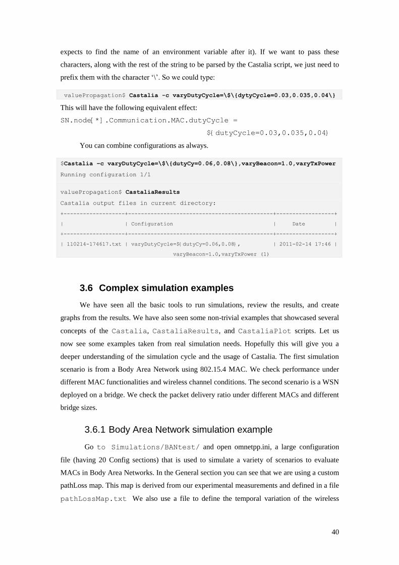
40
expects to find the name of an environment variable after it). If we want to pass these
characters, along with the rest of the string to be parsed by the Castalia script, we just need to
prefix them with the character „\‟. So we could type:
valuePropagation$ Castalia -c varyDutyCycle=\$\{dytyCycle=0.03,0.035,0.04\}
This will have the following equivalent effect:
SN.node[*].Communication.MAC.dutyCycle =
${dutyCycle=0.03,0.035,0.04}
You can combine configurations as always.
$Castalia –c varyDutyCycle=\$\{dutyCy=0.06,0.08\},varyBeacon=1.0,varyTxPower
Running configuration 1/1
valuePropagation$ CastaliaResults
Castalia output files in current directory:
+-------------------+---------------------------------------------+------------------+
| | Configuration | Date |
+-------------------+---------------------------------------------+------------------+
| 110214-174617.txt | varyDutyCycle=${dutyCy=0.06,0.08}, | 2011-02-14 17:46 |
varyBeacon=1.0,varyTxPower (1)
3.6 Complex simulation examples
We have seen all the basic tools to run simulations, review the results, and create
graphs from the results. We have also seen some non-trivial examples that showcased several
concepts of the Castalia, CastaliaResults, and CastaliaPlot scripts. Let us
now see some examples taken from real simulation needs. Hopefully this will give you a
deeper understanding of the simulation cycle and the usage of Castalia. The first simulation
scenario is from a Body Area Network using 802.15.4 MAC. We check performance under
different MAC functionalities and wireless channel conditions. The second scenario is a WSN
deployed on a bridge. We check the packet delivery ratio under different MACs and different
bridge sizes.
3.6.1 Body Area Network simulation example
Go to Simulations/BANtest/ and open omnetpp.ini, a large configuration
file (having 20 Config sections) that is used to simulate a variety of scenarios to evaluate
MACs in Body Area Networks. In the General section you can see that we are using a custom
pathLoss map. This map is derived from our experimental measurements and defined in a file
pathLossMap.txt We also use a file to define the temporal variation of the wireless

41
channel also derived from our measurement campaigns (section 4.1 provides more details
about the format and meaning of these files).
All scenarios use the throughputTest application, where all nodes send packets
to a sink/hub node at a constant (configurable) rate. The hub is node 0. Have a look at the
summary of the configurations:
Castalia/Simulations/BANtest$ Castalia
List of available input files and configurations:
* omnetpp.ini
General
ZigBeeMAC
GTSon
GTSoff
noTemporal
BaselineMAC
pollingON
pollingOFF
naivePolling
minScheduled
maxScheduled
varyScheduled
varyRAPlength
oneNodeVaryRate
oneNodeVaryPower
oneNodeVaryTxNum
allNodesVaryRate
setRate
setPower
allNodesVaryPower
varyReTxNum
You can see that there are two basic MACs: Zigbee and BaselineMAC. We can vary
the packet rate, the Tx power, the retransmission attempts, in one node or all the nodes. We
can vary parameters of the MACs relating to scheduled access, random access and improvised
access (polling). We can also choose a wireless channel with no temporal effects.
For the example in this section we will concentrate on ZigbeeMAC (or more
accurately IEEE 802.15.4 MAC). Let‟s run a simulation testing how Zigbee performs when

42
its Guaranteed Time Slot (GTS)8 functionality is turned on or off and also when we are
having a wireless channel that exhibits temporal pathloss variation vs. one that it does not9.
For all of these 4 scenarios we will vary the packet rate of the sending nodes. We also run
every scenario with 5 different seed sets.
BANtest$ Castalia -c
ZigBeeMAC,allNodesVaryRate,[GTSon,GTSoff][noTemporal,General] -r 5
Running configuration 1/4
Running configuration 2/4
Running configuration 3/4
Running configuration 4/4
BANtest$ CastaliaResults -i 101221-191001.txt
+-------------------+-----------------------------------------+------------+
| Module | Output | Dimensions |
+-------------------+-----------------------------------------+------------+
| Application | Application level latency, in ms | 1x1(31) |
| | Packets received per node | 1x5 |
| Communication.MAC | Fraction of time without PAN connection | 5x1 |
| | Number of beacons received | 5x1 |
| | Number of beacons sent | 1x1 |
| | Packet breakdown | 5x1(5) |
|Communication.Radio | RX pkt breakdown | 6x1(5) |
| | TXed pkts | 6x1 |
| ResourceManager | Consumed Energy | 6x1 |
| wirelessChannel | Fade depth distribution | 1x1(14) |
+-------------------+-----------------------------------------+------------+
We see the rich output produced by the simulation. Let‟s look at the packets received
by the application (and let‟s draw a graph since text would be too hard to follow):
/BANtest$ CastaliaResults -i 101221-191001.txt -s packets |
CastaliaPlot -o zigbee-ban-app-4types.png -l bottom
8 GTS is a TDMA-based scheme that 802.15.4 is using. In our particular simulation scenario, each
round has 16 slots. Each of the 5 nodes is requesting and getting 3 slots, thus 15 slots in total are
devoted to TDMA. The remaining slot is always the first slot after the beacon, and is using a contention
based scheme. When GTS is off then all 16 slots are using contention-based access.
9 The General configuration describes a wireless channel with temporal variability so we are using
“General” config to describe a temporal channel (vs. the noTemporal config which describes a non
temporal channel)

43
The y axis is average packers received per node (only node 0 receives packets but it
receives them from multiple nodes, this is what the “per node” means). The x axis is the
sending rate for each node measured in packets/sec. Nodes are sending packets for 50 secs so
if we had perfect reception we would reach 1500 packets per node for the 30packets/sec/node
case. Notice that for low traffic the GTSon noTemporal curve achieves the maximum (e.g.,
16packets/sec/node 800packets received per node). Generally the protocol performs better
when the GTS is turned on. This is something to be expected as TDMA schemes make a more
efficient use of the wireless medium and are reducing interference. We also notice that the
performance (packets received) is better when the channel has no temporal variation. Again
this is to be expected as the temporal variation introduces some deep fades that break the
connectivity between the sender nodes and the hub, whereas with the no temporal pathloss
variation the links are kept in a relatively good state for our specific example. Finally notice
that as the traffic rate reaches the larger volumes we start seeing early indications of
saturation, especially for the GTSoff General case.
We run the scenarios for 5 seed sets. The confidence levels calculated are quite tight
but it would be good to see the variability of results and investigate how reasonable they look.
For that reason we use the --all switch and draw the four individual curves.
BANtest$ CastaliaResults -i 101221-191001.txt -s packets --all -f
"GTSoff,General" | CastaliaPlot -o zigbee-ban-app-GTSoff,General.png
-l bottom --colors r

44
/BANtest$ CastaliaResults -i 101221-191001.txt -s packets --all -f
"GTSoff,noTemporal" | CastaliaPlot -o zigbee-ban-app-
GTSoffno,Temporal.png -l bottom --colors g
BANtest$ CastaliaResults -i 101221-191001.txt -s packets --all -f
"GTSon,General" | CastaliaPlot -o zigbee-ban-app-GTSon,General.png -
l bottom --colors b
BANtest$ CastaliaResults -i 101221-191001.txt -s packets --all -f
"GTSon,noTemporal" | CastaliaPlot -o zigbee-ban-app-
GTSon,noTemporal.png -l bottom --colors m
There is some variability of results. Remember each point is a result from an
individual seed set but also from an individual node, and since the nodes have different path
losses to the hub (due to the use of our experimental pathloss map) we can expect different
performances from different nodes. This is especially true when we have temporal variation
and these path losses differences manifest themselves as different probabilities of link
outages. Generally the variability appears reasonable, with the possible exception of a few
low points at high rates in GTSon,General. We can delve into the different aspects of the
results to try and explain the full behaviour and at the end we can consult individual run
traces. Let us start by looking at the application-level latency histograms for some cases:
BANtest$ CastaliaResults -i 101221-191001.txt -s latency -f
GTSoff.*=24 | CastaliaPlot -o zigbee-ban-app-latency-GTSoff.png --
yrange 1200 --xrotate 90 -s histogram
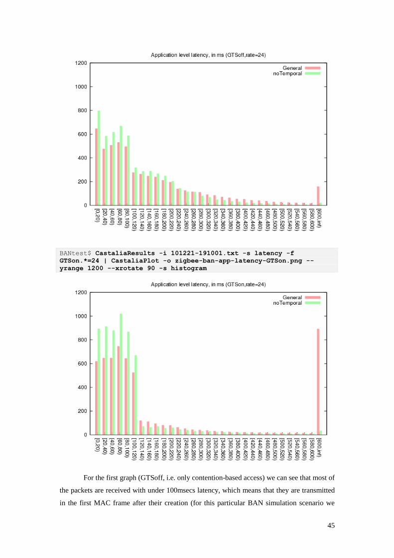
45
BANtest$ CastaliaResults -i 101221-191001.txt -s latency -f
GTSon.*=24 | CastaliaPlot -o zigbee-ban-app-latency-GTSon.png --
yrange 1200 --xrotate 90 -s histogram
For the first graph (GTSoff, i.e. only contention-based access) we can see that most of
the packets are received with under 100msecs latency, which means that they are transmitted
in the first MAC frame after their creation (for this particular BAN simulation scenario we

46
have chosen the MAC frame to be 120ms). We also see that no temporal is performing better
as expected. The non-negligible portion of packets at the [600..inf) bucket is a sign of
oncoming saturation for the temporal case (General). For the second graph (GTSon) we see
even more pronounced effects. The majority of the packets are received within the first frame
of creation and we also see a big portion of packets with large delay. This tells us that there is
potential saturation in this case, with overflown buffers, possibly explaining some of the low
performance points in the “packets received per node” graph.
To further investigate we can look at the breakdown of packets at the MAC level:
BANtest$ CastaliaResults -i 101221-191001.txt -s "Packet break" -f
GTSoff -p | CastaliaPlot -o zigbee-ban-mac-GTSoff-percentage.png -s
stacked --colors b,dc,pi,y,o,r -l "outside width -7" --xrotate 90 --
order-columns=5,6,4,3,2,1 --yrange 1.05
This is a nice example of using CastaliaResutls and CastaliaPlot to achieve an elegant
and informative graph. Notice how we show the results that match “Packet break”, how we
filter to show only rows with “GTSoff” and how we the results are shown as fractions of 1 (-p
option). Notice also we choose the colors and reorder the columns to get the aesthetic result
we wish.
Looking at the graph we can get an immediate feeling on how better the noTemporal case is.
We also see that the main difference is a portion of the packets who failed because of no Ack
was received (a direct result of the deep fades in the channel and loss of connectivity). For
high rates we also see more packets being overflown. This breakdown is for packets sent at

47
the MAC level. We can also look at the breakdown of packets received at the Radio layer of
node 0 (the hub).
BANtest$ CastaliaResults -i 101221-191001.txt -s RX -f
GTSoff.*node=0 -p -n | CastaliaPlot -o zigbee-ban-radio0-GTSoff-
percentage.png -s stacked -l "outside width-7" --yrange 1.05 --
order-columns 5,4,1,2,3 --colors dg,g,r,pi,b --xrotate 90
Notice how we are have to break the results per node (using –n) to get the radio layer
of just node 0 and the more advanced filtering we do.
The graph verifies our assumptions for the cause of noAck packets from the previous
graph. Although the packets that are interfered do not increase much in the General (i.e.
temporal) case, we see a portion of packets failing due to very low received signal. This
category does not even exist in the noTemporal case. We also see a small portion of packets
that fail due to radio of node 0 being in the wrong state. In our particular case this can only
mean that the radio is TXing yet the carrier sensing mechanism in other nodes is not effective.
This hypothesis needs to be confirmed by looking at the traces.
Let us look also at the GTSon case (TDMA-based access) too:
BANtest$ CastaliaResults -i 101221-191001.txt -s "Packet break" -f
GTSon -p | CastaliaPlot -o zigbee-ban-mac-GTSon-percentage.png -s
stacked --colors b,dc,pi,y,o,r -l "outside width -7" --xrotate 90 --
order-columns=5,6,4,3,2,1 --yrange 1.05
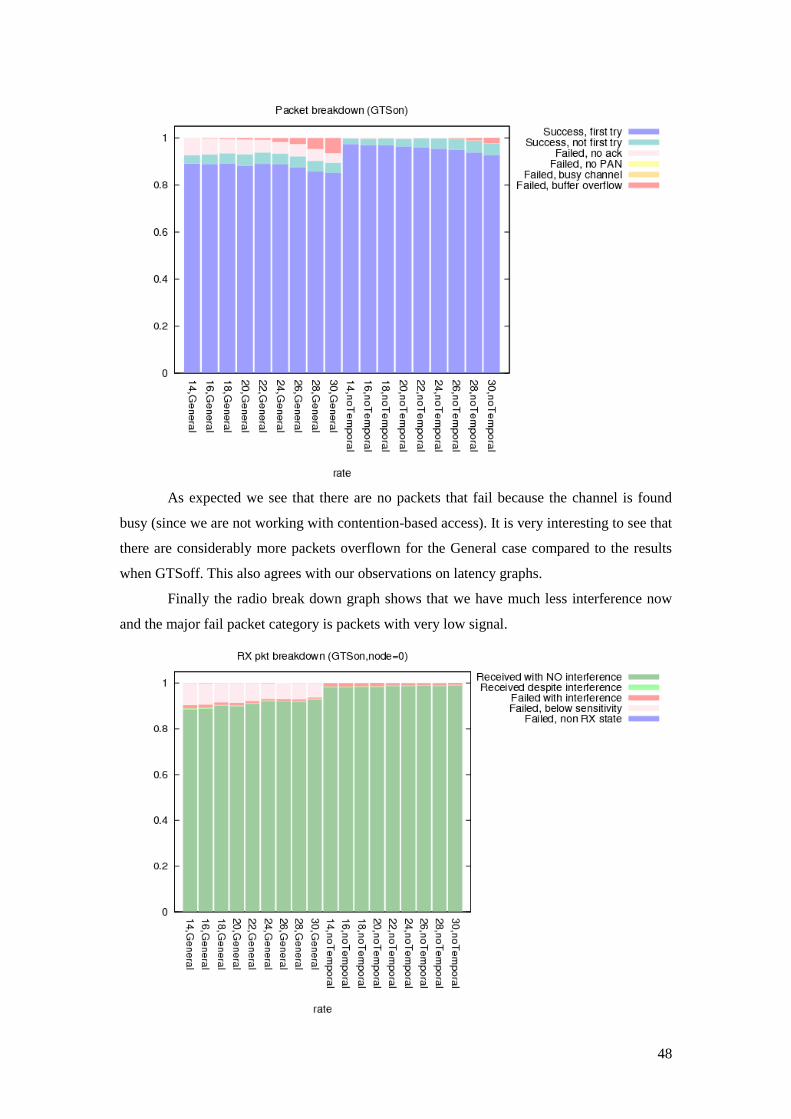
48
As expected we see that there are no packets that fail because the channel is found
busy (since we are not working with contention-based access). It is very interesting to see that
there are considerably more packets overflown for the General case compared to the results
when GTSoff. This also agrees with our observations on latency graphs.
Finally the radio break down graph shows that we have much less interference now
and the major fail packet category is packets with very low signal.
49
3.6.2 Bridge Test simulation example
This simulation scenario was created to test some basic aspects of a WSN used for
structural health monitoring of a bridge. It has the following characteristics:
The sensing nodes are placed in a grid throughout the simulation field within 20 meters
from each other. The sink node is located in the middle of the field, and all sensing nodes will
try to deliver their reports to the sink. Every 5 minute (on average) a car appears in the
simulation field (CarsPhysicalProcess is used, which creates objects moving in lines). A
passing car is guaranteed to trigger all sensing nodes along its path, thus creating a traffic
flow towards the sink node in the network. But not all nodes are triggered for the same
amount of time; node on the central line of the deck spend more time above the triggering
threshold. Additionally, the sink node will be distributing several packets [totalling 5Kbytes]
to all sensing nodes at the beginning of the simulation and then repeat doing so every day of
the simulation. These packets symbolize an update software patch.
The goal of this scenario is to evaluate the performance of such WSN with different
parameters in MAC and Routing layers, as well as different sizes of the bridge being
monitored. In release 3.1, the results from the BridgeTest simulation scenario are not very
exciting since we are missing crucial routing functionality. The old tree-based routing present
in version 2.3b is no longer available and the multipathRings routing does not seem to
perform well. Thus we are simply using noRouting (some sort of app level broadcast is
performed to dispense the results). The simulation scenario is interesting though because of
the way we define different network sizes (according to the bridge size).
Open the omnetpp.ini file and look at the configurations. Notice how we are creating
the various deployments for different bridge sizes:
[Config 100mBridge]
SN.field_x = 100
SN.field_y = 20
SN.deployment = "[0]->center;[1..18]->6x3"
SN.numNodes = 19
SN.physicalProcess[0].point1_x_coord = 0
SN.physicalProcess[0].point1_y_coord = 10
SN.physicalProcess[0].point2_x_coord = 100
SN.physicalProcess[0].point2_y_coord = 10
We have to set the correct field size, the correct number of nodes, and the correct
deployment (proper grid size). Node 0 (the sink) always goes at the centre. Then we need
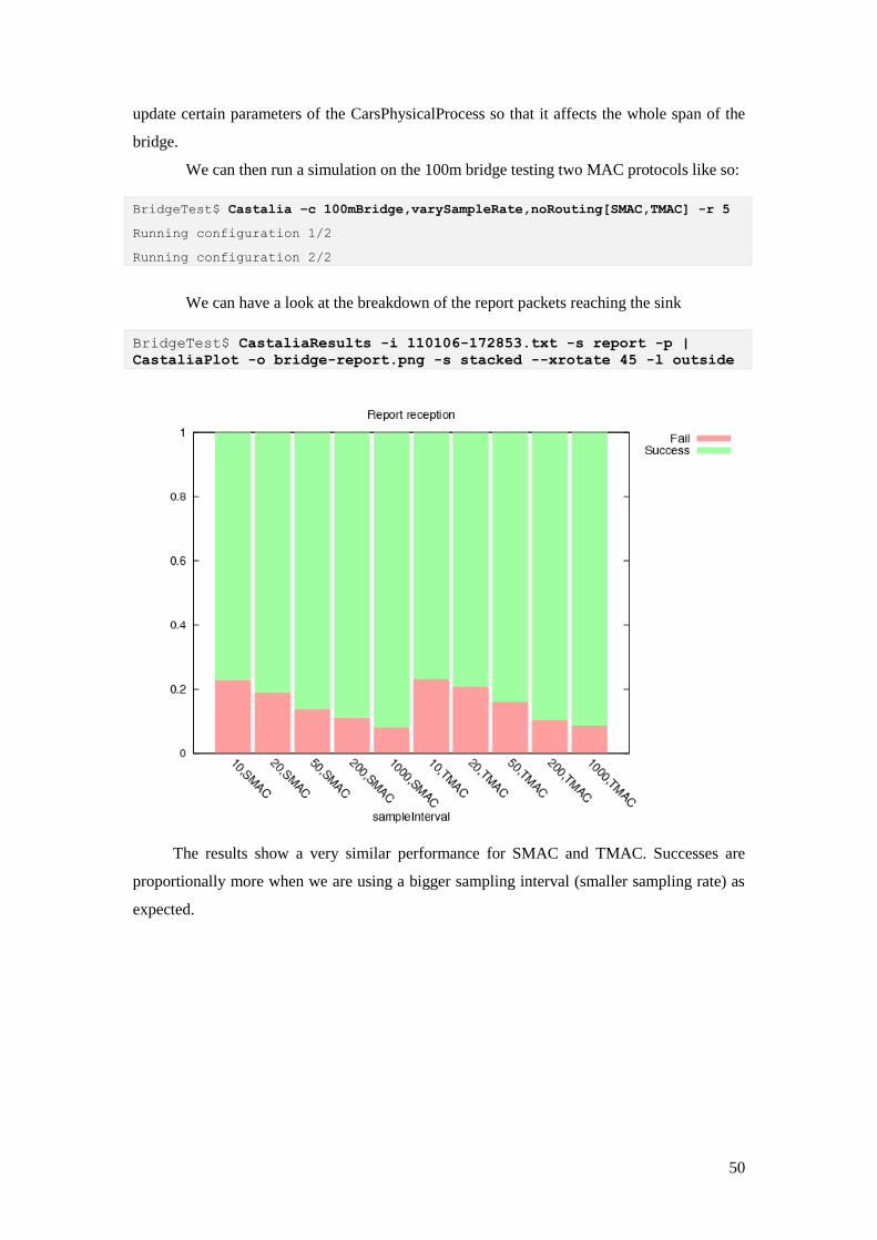
50
update certain parameters of the CarsPhysicalProcess so that it affects the whole span of the
bridge.
We can then run a simulation on the 100m bridge testing two MAC protocols like so:
BridgeTest$ Castalia –c 100mBridge,varySampleRate,noRouting[SMAC,TMAC] -r 5
Running configuration 1/2
Running configuration 2/2
We can have a look at the breakdown of the report packets reaching the sink
BridgeTest$ CastaliaResults -i 110106-172853.txt -s report -p |
CastaliaPlot -o bridge-report.png -s stacked --xrotate 45 -l outside
The results show a very similar performance for SMAC and TMAC. Successes are
proportionally more when we are using a bigger sampling interval (smaller sampling rate) as
expected.

51
4 Modeling in Castalia
This chapter explains how Castalia models the different aspects of a wireless sensor
network from communications to physical process. It also gives a detailed account of all the
non-composite modules and their parameters. This chapter is your reference to understand
how to use the different modules and what you can do with them. The single common thing
that we can mention for all non-composite modules in Castalia is that they all have a
parameter called collectTraceInfo. This is set by default to „false‟. If set to „true‟, the
module will produce trace information that will be written in the Castalia-Trace.txt file. We
have already seen examples of this in Chapter 3.
Communications is the most carefully modeled aspect of the Castalia simulator. From
the wireless channel to the radio behavior and the implementation of different MAC
protocols, we tried to capture the essence and many details of their real counterparts.
4.1 The Wireless Channel
The wireless channel is a notoriously difficult medium to model, especially when taking
into account mobile nodes, a changing environment (e.g., in the BAN case: the body moving)
and broadband communications. Even though there is a big corpus of theoretical results and
experimental measurements for wireless communication in general, they tend to practically
affect areas with more commercial impact such as cellular communication, and recently
WiMAX. The mobile ad hoc networks and wireless sensor networks have not gained as much
from the modeling advances of wireless communication. There are multiple reasons for this,
the main ones being: 1) more complicated problem, 2) comparatively smaller immediate
tangible commercial benefits to allow for the expensive and tedious job of detailed
measurements and modeling, and 3) researchers coming mostly from the CS, networking
background, lacking deep knowledge and interest in the physical layer. Nevertheless, some
researchers in the community have taken up the much needed role and have produced models
that fit experimental data, at least for some important aspects. The recent interest with Body
Area Networks and the upcoming IEEE BAN standard has created another important
momentum. For example, at NICTA, we have created experimental testbeds to capture
hundreds of thousands measurements. Those measurements are analyzed to provide accurate
models for both the average path losses around the body, and more importantly, the temporal
variation behaviour of the channel.
We are confident to claim that, concerning the wireless channel, Castalia is the most
realistic simulator one could find for WSN and BAN. The word “realistic” here is used in the
sense that the simulator is making the necessary provisions to capture various important

52
features of the wireless channel. In order to have results that accurately reflect reality one
would need appropriate input parameters and input files. In simple words, one needs to “tune”
the simulator right. In the simulation examples provided with the distribution of Castalia,
many of the parameters are set at reasonable values that reflect some real situation, some
though –especially large input files modeling temporal variation– are not freely available and
are NICTA‟s intellectual property. NICTA is interested in various forms of collaboration, so
you are welcome to contact us regarding more accurate input files.
4.1.1 Average path loss modeling
One important aspect of the wireless channel modeling is to estimate the average path
loss between two nodes, or in general, two points in space. For WSN, where the separation of
nodes is from a couple of meters to a hundred meters, the lognormal shadowing model has
been shown10
to give accurate estimates for average path loss. This is the formula that returns
path loss in dB as a function of the distance between two nodes and a few parameters
Xd
ddPLdPL
0
0 log10)()(
PL(d) is the path loss at distance d, PL(d0) is the known path loss at a reference distance
d0, η is the path loss exponent, and Xσ is a gaussian zero-mean random variable with standard
deviation σ. The four parameters in italics and bold, are defined as parameters of the wireless
channel module. Looking into src/wirelessChannel/WirelessChannel.ned
double pathLossExponent = default (2.4);
double PLd0 = default (55);
double d0 = default (1.0);
double sigma = default (4.0);
To access these parameters in an .ini file you have to prefix their name with
“SN.wirelessChannel.”
The lognormal shadowing model is not very accurate if you want to capture the
correlation between the two directions of a link11
. If you treat the two directions as
independent links, the variance you get is much larger than the one experienced in reality.
For this reason we are using the model to return an average path loss for both directions of a
link and then we add and subtract a separate Gaussian zero-mean random variable with
10 Zuniga et. al. [4] have shown that the observed Packet Reception Rates (PRR) in experimental setups
with mica2 motes can be explained with the lognormal shadowing channel model and appropriate
models for the radio modulation (which Castalia uses).
11 A link here is just a pair of nodes or more generally two points in space.

53
standard deviation SN.wirelessChannel.bidirectionalSigma. This standard
deviation should generally be small (default = 1.0). This parameter replaces the old parameter
SN.wirelessChannel.allBidirectionalLinks, which was a much coarser attempt to capture
correlation between the two directions of a link. Now, with the new parameter we have a
more clean and independent way to control correlation between the two directions.
If we are concerned with BAN modeling, the lognormal shadowing model does not
produce good results. In this case, we can use another option that Castalia gives us and that is
to explicitly set our path loss map. For example, we might have measured average path losses
using a testbed (as we do at NICTA) and provide these as input to Castalia. This is done
through the SN.wirelessChannel.pathLossMapFile parameter which gives the
filename of the specially formatted input file.
The input file has lines of the following format:
TxNodeID>RxNodeID1:dB_value,RxNodeID2:dB_value,…
example: 0>1:56,2:40,3:59,4:54,5:58
This means that when node 0 is transmitting, node 1 is experiencing 56dB path loss,
node 2 is experiencing 40dB loss, node 3 a 59dBm loss, etc.
Before Castalia 3.0 we also provided another option: to give a map of packet reception
probabilities (also called packet reception rates: PRR) using the
SN.wirelessChannel.PRRMapFile parameter. This is no longer an option because of
changes in the radio model. Now the radio can dynamically change its modulation type, plus
we can have multiple kids of radios operating in a network. To translate a PRR to a path loss
in dB, you need to know the operation parameters of the radios involved. If you can have
different and dynamically changing radio operating parameters it makes little sense to
determine a wireless channel with a PRR map. Thus, the PRRMapFile parameter is now
obsolete.
4.1.2 Allowing for node mobility
Allowing for mobile nodes, complicates matters, since now it is not enough to take the
average path losses between the nodes. We need to keep state about path losses between
points in the space. This implies that we need to break up the space in discrete cells and
calculate the path losses from each cell to each other cell. Look at figure 4 for an example of
such a map only for one transmitting cell.

54
Figure 4: Path loss map in a 2D space segmented in cells (for a single transmitter cell)
The map is calculated with the model or input files we described before, we just take
cell locations and cell IDs instead of specific node locations and node IDs. The parameters
SN.wirelessChannel.xCellSize, SN.wirelessChannel.yCellSize,
SN.wirelessChannel.zCellSize set the cell size (default = 5m). The smaller it is,
the more fine-grained and accurate is your path loss map but also the more memory is needed
to store it. Imagine you just have a 2-dimentional field 100m by 100m and you would like to
have a cell of 1m y 1m, this results in 10,000 cells. This in turn results in 10,0002 =
100,000,000 path losses. With several bytes per path loss element (we store information
besides the path loss) this can mean GBytes of memory. Our algorithm is smart and does not
keep all possible combinations, but you get the idea on how fast can the state-space explode
and also the processing time searching through these cells. Adding a 3rd
dimension can
aggravate matters, so be aware of the values you give to these parameters. In the wireless
channel trace messages there is information about the size of the path loss map and the time it
took to initialize it. This information can help you decide whether your choice of cell size
with respect to the field is memory- and computation- efficient. Another parameter related to
mobility in the wireless channel is SN.wirelessChannel.onlyStaticNodes. If we
do not have any mobility in our scenario then we can declare this parameter true and save a
lot of memory space and computation time. In this case, the space is not broken up into cells
(the cell parameters do not matter) and the exact node locations are used in path loss
computations much like Castalia 1.3 and below did.
Generally in Castalia, the modeling and computations are based on cells. When we do
not have mobility, the nodes are treated as special cells where their location is acquired in a
different manner, but all the rest of the code remains the same.

55
4.1.3 Temporal variation modeling
Another very important aspect of the wireless channel is the temporal variation. This
is especially pronounced in rapidly changing environments as those experienced in a BAN.
Figure 5 shows a typical profile of channel variation. Notice the sharp drops (measured up to -
50dB in our BAN experiments) and that most of the time the channel is below the average
path loss (0dB) (e.g., 2/3 of the time in Weibull fading channels). There are several theoretical
models to describe temporal variation, taking their names from corresponding complex
distributions (e.g., Rayleigh, Weibull, Nakagami, Gamma, lognormal). From our
measurements around the human body we have seen that no single model describes temporal
variation best. For that reason we tried to keep our modeling general but still expressively
powerful to describe any temporal variation the measurements were showing.
Figure 5: Typical temporal fading in wireless
In Castalia when we have to calculate the path loss at a specific moment, we first find
the average path loss from the state we have stored during channel initialization (i.e., building
the path loss map either using the model or the input files, as described in section 4.1.1) and
then we have to find the component of the path loss due to temporal variation. To do this we

56
have kept the last “observed” value (in reality the last value we computed) and the time it has
passed since then. These two numbers should define a probability density function (pdf) that
we draw our new value from. Obviously, if little time has passed, then the bulk of the
probability in this pdf should be in values close to the last observation. If the last observation
is a deep fade (e.g. -40 dB) then the pdf should “boost” bigger values. The problem is that we
cannot produce those pdfs dynamically from a model. They have to be produced from our
experimental measurements. This in turn implies that we cannot have a pdf for any
combination of last observation (dB value) and time passed. Instead we have to declare for
what dB values and what times we are providing the pdfs. Then find a way to describe the
pdfs in a manner that is accurate enough and computationally cheap. All this is done in a
specially formatted file. The.ini file parameter is -as you have probably guessed- is the name
of that file: SN.wirelessChannel.temporalModelParametersFile
The file is formatted in the following way: (strings min_value, step, max_value, t1,
t2, tn, and T should be replaced with floating point numbers. The expression{pdf description}
is explained shortly after.
Signal variability (dB): min_value:step:max_value
Correlation times (msec): t1,t2,…tn
Coherence time (msec): T
T: {pdf description}
tn,min_value: {pdf description}
tn,min_value+step: {pdf description}
tn,min_value+2step: {pdf description}
…
tn,max_value: {pdf description}
tn-1,min_value: {pdf description}
…
tn-1,max_value: {pdf description}
…
t1,max_value: {pdf description}
So the file describes the values and times it will provide pdf descriptions for, and then
gives these pdf descriptions. It also gives an extra time which we call “coherence time” (in
lieu of a better name) and an extra pdf for it. This is a large time, beyond which, it does not
matter what was the last observed value and we just draw our number from its corresponding
pdf.

57
Now, what is the pdf description? It is a generic way to describe any pdf (in a
quantized way) that also makes drawing a number from it computationally fast. In its simplest
form is an array of dB values, say 100 values, space-separated. To draw a number, we pick a
random number between 1 and 100, and then we draw the value with the same index. In that
way we can arbitrarily describe any pdf (within some accuracy). For example, let‟s take a
smaller array with just 10 values (thus when drawing a value we pick a random number
between 1 and 10): 23 -23 -23 -23 -23 10 10 10 -5 15. This describes a pdf
where value -23 has probability 0.5, value 10 has probability 0.3, and 0.1 probability for
values -5 and 15. Now you understand that we are loosing some accuracy because of the
limited number of values we have (if we have 100 values we are limited to probabilities of
0.01). The tails of the distributions we are concerned with are important though, so we need to
capture their values which correspond to really small probabilities. We could increase the
number of values we have to 1000 or 10,000 and allow for many duplicate values, but this
would be a waste of memory. There is a more elegant way to do it that incurs an almost
insignificant increase in computation time. We can define levels of draws. So at the top level
we may have 10 buckets (usually filled with values), which all represent 0.1 probability. One
of these buckets instead of having a value it can have a letter, that points is to the next level. If
we the random number we pick chooses the letter, then we have to draw again from another
array of values/letters. So if the second level has 5 values then each of these values has 1/10
* 1/5 = 0.02 probability. An example looks like this:
23 -23 -23 -23 -23 10 10 10 -5 A; A= 15 15 15 3.5 3.5
This defines a pdf very similar to the example before but now value 15 has
probability 0.06 and there is a new value 3.5 with probability 0.04.
This is the general expression for {pdf description} ([] means optional):
pdf:= level; [letter= level;] ... [letter= level]
level:= number ... number [letter] ... [letter]
There is a limit to the depth of levels that we can define, but for most practical
reasons there is no point in going beyond level 3 or 4. In the temporal parameters file we give
with the BANtest scenario we have taken a range -31:1:11, times of 1000ms, 250ms, 10ms
which results in 129 pdfs. Our pdfs have 2 levels with 101 buckets in the first level and 10 in
the second. We also have coherence time = 5secs and a 2 level pdf with 1001 buckets in the
first level and 10 in the second. The total file size is 118Kbytes.

58
4.1.4 Delivering signals to the Radio module
In Castalia versions earlier than 3.0, the wireless channel was responsible for
calculating the interference a receiver “sees”, calculate the SINR (signal to interference plus
noise ratio) and based on radio parameters decide whether a packet will be successfully
received. If yes, then it would send the packet to the radio. So the wireless channel module
was delivering packets to the radio of nodes. This modeling worked fine but it did not allow
for multiple radio modes to co-exist in a network. Furthermore, it made fine-grain dynamic
interference calculation challenging. Since Castalia 3.0 and the complete restructuring of the
radio model, we were able to revisit the operation of the wireless channel too. Now the
wireless channel just sends the signal to the radio and lets the radio calculate its interference,
its (dynamically changing) SINR and decide whether or not it receives a packet. So now the
wireless channel just needs to send messages to the radio that carry information about the
signal, such as: modulation, bandwidth, carrier frequency, and most importantly, the strength
of the signal in dBm. Based on the path loss (average path loss + temporal variation) and the
transmission power of a transmitter, the wireless channel can calculate the signal strength
received at a node.
Which signals do we send to a radio module? All of them, irrespective of how weak
they are? That would be a waste of resources; both computation time and memory. A signal
transmission would result to a signal reception in all existing nodes irrespective of how far
they are from the sender. Moreover if we have mobility, one cell would affect all other cells,
resulting in the biggest possible path loss maps. Instead we can be smarter and set a signal
strength threshold that beneath it does not make sense to deliver a signal. What would this
threshold depend on? Obviously, the radio sensitivity. Should it just be the radio sensitivity?
No, because a signal can be weaker than the radio sensitivity but it can still cause interference
to another signal. Imagine two signals being heard at a receiver, one is at the sensitivity
threshold, the other is 1dB smaller. If we did not deliver the smaller signal, the first one
would be processed and the packet that it carried would be received with no problems. If we
deliver both signals, a collision would probably occur. So how much lower than the radio
sensitivity should we go? 10dB is usually more than enough and 5dB should be the minimum.
Because there are tradeoffs at play we decided to make the signal delivery threshold a
parameter of the wireless channel.
double signalDeliveryThreshold = default (-100);
-100dBm is a good value for both the BAN radio and the CC2420 we have defined. If
you are using CC1000 then you should probably choose -103 or lower.

59
4.1.5 Choosing naive models
It would be useful to define simpler models (up to the rather simplistic disk model) so
that simulation results can be compared with results from other simulators and more
importantly so that the user can test different hypotheses on why a distributed algorithm does
not work (or underperforms) when more realistic assumptions are taken into account . This is
especially true with models of communication, especially the lower-level ones (channel and
radio).
In an omnetpp.ini file, we can make the wireless channel simpler by simply setting:
SN.wirelessChannel.sigma = 0
SN.wirelessChannel.bidirectionalSigma = 0
This way all nodes at a certain distance from a transmitter get the exact same signal
strength and all links are perfectly bidirectional (i.e., the quality of AB is the same as the
quality of BA).
If we can also provide sharp thresholds for the radio reception (i.e., perfect reception of
a packet or no reception at all) then we end up with the simple unit disk model. Indeed, for all
the radios we have defined, we provide a special mode with an ideal modulation scheme. To
choose it, simply set:
SN.node[*].Communication.Radio.mode = "IDEAL"
So by setting the two sigmas of the wireless channel to 0 and the radio mode to
“IDEAL” a user can emulate the naïve -but still prevalent- unit disk communication mode
(i.e., transmissions within a certain range from a transmitter are perfectly received, and
outside this range not received at all).
When adopting a unit disk model, a user can control the range of the disk by controlling
the SN.wirelessChannel.PLd0 parameter. Assume you need the range of the disk to
be 50m then you should set PLd0 = (TxPowerUsed_dBm – max(receiverSensitivity,
noisefloor+5dBm) ) – 10*pathLossExponent*log(50) 12
The user can further play with the collisionModel parameter of the Radio module
to get simpler models. We will explain this in the section 4.2.3.
12 In the radios we have defined so far, SN.node[*].Communication.Radio.receiverSensitivity is greater
or equal to (SN.node[*].Communication.Radio.noiseFloor +5dBm)

60
4.2 The Radio
The radio module tries to capture many features of a real low-power radio, one that is
likely to be used in wireless sensor network platforms. The main features of our Radio
module are:
Multiple states: transmit, receive/listen, multiple (configurable) sleep states
Transition delays from one state to another.
Multiple (configurable) transmission power levels
Different power consumption for the different states and Tx levels used.
Multiple modes of operation (defined by modulation, datarate, bandwidth, noise
floor, and other parameters) that can dynamically change.
Multiple modulation schemes natively supported (FSK, PSK, DiffQPSK,
DiffBPSK, Ideal modulation with 5dB threshold).
Ability to define custom modulation schemes by defining SNR BER mapping
Continuous calculation of RSSI (Received Signal Strength Indicator)
CCA (Channel Clear Assessment) capability; interrupts to the MAC module.
Fine-grain interference calculation (dynamically changing during packet
reception) and calculation of exact bit errors in a packet
4.2.1 The Radio Parameters file
To define the main operating parameters of a radio we are using a file which follows a
specific format. We have already defined 3 radios that you can find in
Simulations/Parameters/Radio/. These are: BANRadio.txt CC1000.txt
CC2420.txt. BANRadio describes the narrowband radio proposed in the IEEE 802.15
Task Group 6 documents. CC2420 and CC1000 define the real radios of the same name by
Texas Instruments. The parameter RadioParametersFile of the Radio module points to
this file. The module will read it and parse it. Here is the format of a Castalia Radio
Parameters file:
Any line beginning with „#‟ is considered a comment.
The files should contain 5 sections each starting with the line
RX MODES
TX LEVELS
DELAY TRANSITION MATRIX
POWER TRANSITION MATRIX
SLEEP LEVELS

61
The sections can appear in any order. In the radios we have defined, we follow the
order shown above. Section RX MODES contains one or more lines of the following format:
Name, dataRate(kbps), modulationType, bitsPerSymbol, bandwidth(MHz),
noiseBandwidth(MHz), noiseFloor(dBm), sensitivity(dBm), powerConsumed(mW)
All quantities are numbers except from Name, which is an arbitrary string and
modulationType which can take only the following values: FSK, PSK, DIFFBPSK,
DIFFQPSK, IDEAL, CUSTOM. Here‟s an example from CC2420.txt:
normal, 250, PSK, 4, 20, 194, -100, -95, 62
Section TX_LEVELS should have two lines. The first line starts with the string
“Tx_dBm” followed by n numbers (space-separated). The second line starts with the string
“Tx_mW” also followed by n numbers separated by at least one space. As you can
understand, the first line lists the output power of the different transmission levels in dBm and
the second line how much energy the radio is spending when transmitting in a power level.
The order of the power levels should be kept the same in both lines. In the radio files we have
already defined, we chose to go from larger to smaller. Here‟s an example from CC2420.txt
defining the 8 possible transmission power levels:
Tx_dBm 0 -1 -3 -5 -7 -10 -15 -25
Tx_mW 57.42 55.18 50.69 46.2 42.24 36.3 32.67 29.04
Section DELAY TRANSITION MATRIX specifies delays (in msec) to switch between
the three main radio states: RX (receive), TX (transmit) and SLEEP. This section should
contain a line corresponding to (and starting with the name of) each state. Following the name
of a state there are three numbers defining transition times in milliseconds from RX, TX and
SLEEP states respectively to the current state given first in each line. Below is an example
from CC2420.txt:
RX - 0.01 0.194
TX 0.01 - 0.194
SLEEP 0.05 0.05 -
In this case, it takes the radio 194μsec to change from SLEEP state to either RX or TX,
10μsec to change between TX and RX states and 50μsec to enter the SLEEP state. Note that
each line contains „-„ instead of a number in the cells corresponding to no transitions.

62
Similarly to the previous section, POWER TRANSITION MATRIX section follows
the same format to specify the consumed power (in mW) during the time when state
transitions are taking place. In CC2420.txt configuration it can be seen that transitions to
SLEEP state consume 1.4mW while any other transitions take 62mW:
RX - 62 62
TX 62 - 62
SLEEP 1.4 1.4 -
Lastly, section SLEEP LEVELS defines different sleeping modes (or levels) available
to the radio. Sleep levels exhibit different power consumption. The sleep levels are ordered
from the most “shallow” sleep (i.e., the one with the more power consumption) to the deepest
sleep. While in a sleep level, the radio can only go to the sleep level immediately up or down.
You have to be in the top (shallowest) level to enter the RX or TX state. When going from
RX or TX to sleep, you first go into the shallowest level and gradually go to a deeper sleep
level if desired. These transitions are handled automatically by the radio module. The user
just defines the desired sleep level when the radio is put to sleep and the appropriate
transitions, delays, and power consumption are taken into account. The SLEEP LEVELS
section should contain at least one line of the following format:
Name, power(mW), delay up(ms), power up(mW), delay down(ms), power down(ms)
Name is any string to denote the name of the level and power is the power consumption at
that level. Delay up and delay down denote time taken to move to the level above and below
(which respectively are defined by lines above and below), while values of power up and
down correspond to the energy consumption value during the transition process. In
CC2420.txt only a single sleep level is defined as follows (note that no transition values are
given, since there are no other sleep levels):
idle 1.4, -, -, -, -
4.2.2 Radio Module Parameters
Apart from the Radio Parameters file, the radio module defines a set of parameters that
can be specified from within configuration files (.ini files). The list of these parameters can be
found in the Radio.ned file and is presented below:
string RadioParametersFile = default ("");
This is a path to the radio parameters file as explained in the previous section. The path can be
absolute, or relative to the directory which contains the simulation configuration (.ini) file.
63
string mode = default ("");
This parameter allows us to select the starting RX mode from the list defined in the radio
parameters file. Default value (empty string) means that the first mode listed will be used.
Modes can be changed dynamically during the simulation as will be explained in section
4.2.4.
string state = default ("RX")
This parameter specifies the starting state of the radio once simulation begins. By default the
radio will start in the listening (receiving) state.
string TxOutputPower = default ("");
This parameter defines the starting transmission output power level to be used, e.g. -5dBm.
Note that only power levels that were declared in the radio parameter file can be used. Default
value (empty string) will cause the highest (first) output power level to be used.
string sleepLevel = default ("");
This parameter allows selecting the default sleep level (sleep depth) that will be used by the
radio when a transition to SLEEP state is requested. The default value (empty string) means
that the first level defined will be used. This corresponds to the fastest and most energy
consuming sleep state.
double carrierFreq = default (2400.0);
This parameter allows selecting the starting carrier sense frequency of the radio (in MHz).
int collisionModel = default (2);
This parameter defines the collision model used by the radio to compute the impact of various
incoming signals on each other‟s reception (this process is called interference). More
information on this parameter and various available collision models will be provided in
section 4.2.3
double CCAthreshold = default (-95.0);
This parameter defines the value of Clear Channel Assessment (CCA) threshold used by the
radio when determining whether the wireless channel medium is clear. In particular, if the
RSSI reading (i.e., an estimation of the cumulative power of incoming radio signals) exceeds
this threshold, then the radio will report channel as busy (i.e. not clear).
int symbolsForRSSI = default (8);
This parameter specifies the amount of symbols required by the radio to perform RSSI
calculation.
bool carrierSenseInterruptEnabled = default (false);

64
This parameter allows us to turn on an interrupt capability of the radio module which will
inform upper layers (in particular MAC layer) when the channel state moves from clear to
busy (i.e. when CCAthreshold is passed). This capability is present in some real radios,
however it is turned off by default to ensure that carrier sense interrupt only appears when it is
intended to be used.
4.2.3 Reception and Interference calculation
The Radio module operates on signals that are provided from the wireless channel
module. Section 4.1.4 explained how signals are delivered. Signals last for some time since
they are encoding a packet‟s transmission (OMNeT messages called WC_SIGNAL_START
and WC_SIGNAL_END signify the duration of a signal/packet). Thus, at any time, the radio
module has a list of incoming signals that are affecting each other‟s reception. If a signal is
received without any other signals being received at the same time, then its reception is
decided thus: Based on the noise floor (a parameter of the RX mode of radio operation) and
the received signal strength, we calculate the SNR. Based on the SNR, the modulation
scheme, the data rate, (again, parameters of the RX mode of radio operation) and length of the
packet/signal we calculate how many bit errors has the packet/signal experienced. Based on
the encoding and bit errors, we know if the packet was received correctly. When we add into
the mix interfering signals then we need to calculate the Signal to Interference Ratio (SINR or
SIR) and do the above calculations at every signal change. Bit errors are calculated up to the
point of the last signal change. If a signal changes then we calculate SINR and bit errors for
the last unchanged portion of the packet/signal.
How is interference calculated based on the reception of other signals? We simply add
up the signal strengths of the interfering signals13
. We also add up the power of the thermal
noise (i.e. the noise floor) and we have the SINR.
The user has the option to opt for simpler interference/collision models by setting the
parameter SN.node[*].communication.radio.collisionModel. If set to 0
there are no collisions happening. If set to 1 there is a simplistic model for collisions. In this
case, if two nodes are concurrently transmitting and the receiver can receiver both of their
signals -even minimally- then there is always a collision at the receiver. Notice that for the
same case, with additive interference model, we can have two possibilities: a) have a collision
or b) the receiver receives the stronger of the two transmissions (if it is strong enough). It will
all depend on the specific SIR at the receiver node. Setting the collision model variable to 2
13 Recent research has shown that the total interference is somewhat less that the simple addition of the
interfering signals. In practice, you should not see any difference in the simulation unless you have a
high-interference scenario, where one node is interfered with by 4 or more other nodes each time.

65
uses the additive interference model where transmissions from other nodes are calculated as
interference by linearly adding their effect at the receiver. In chapter 3 you have already seen
the effect of using different collision models in the radioTest simulation scenarios.
4.2.4 Dynamically adjusting radio parameters
Section 4.2.2 illustrated a list of radio module parameters that allow to specify starting
values of radio state, reception mode, sleep level, transmission power output, CCA threshold
and carrier frequency. Values of these parameters can be set in the omnetpp.ini, but what if
we would like to dynamically change the values for some of these parameters within a
specific simulation run? After all, in real platforms, many or the radio parameters are
controllable by the processor. For this purpose we have defined and implemented a function
(overloaded 4 times with 4 different argument sets) called createRadioCommand to assist
with issuing commands to the radio.
First it is important to point out that most communication between Castalia modules is
handled using OMNeT messages. Consecutively, issuing a command to the radio module
involves two steps: 1) create the correct control message (command) and 2) send it to the
right module. Step one is largely automated using one of the createRadioCommand
functions which returns a command ready to be sent. Here are the different forms you can use
the function (they are defined in RadioSupportFunctions.h):
RadioControlCommand
*createRadioCommand(RadioControlCommand_type,double)
RadioControlCommand
*createRadioCommand(RadioControlCommand_type,const char *)
RadioControlCommand
*createRadioCommand(RadioControlCommand_type,BasicState_type)
RadioControlCommand *createRadioCommand(RadioControlCommand_type)
It can be seen that all 4 functions return an object of RadioControlCommand type
that can be transferred between OMNeT modules. Additionally, each function requires a
RadioControlCommand_type argument. This type is defined in the file
RadioControlMessage.msg and can take the following values:
SET_STATE
SET_MODE
SET_TX_OUTPUT
SET_SLEEP_LEVEL
SET_CARRIER_FREQ
SET_CCA_THRESHOLD

66
SET_CS_INTERRUPT_ON
SET_CS_INTERRUPT_OFF
Each of the four functions above is only compatible with a subset of the available
command types, depending on the argument that needs to be provided. More specifically, a
double argument is required for SET_TX_OUTPUT, SET_CARRIER_FREQ and
SET_CCA_THRESHOLD commands. A string (char *) argument is needed for SET_MODE
and SET_SLEEP_LEVEL commands, while a BasicState_type value (corresponding to one
of the 3 radio states – RX, TX and SLEEP) can only be used with SET_STATE command.
Finally, no argument is required for SET_CS_INTERRUPT_ON and
SET_CS_INTERRUPT_OFF radio control commands.
The second step to control the radio is passing the created command to the radio
module. Usually, only two modules that require interaction with the radio: the MAC and the
Application. In the Castalia architecture, the MAC module is connected to the radio module
since they are directly exchanging packets and messages. Consecutively, the MAC module
interface defined in VirtualMac.h file provides a helpful function toRadioLayer() that
allows to send a message (or packet) to the radio. Below are some examples of controlling the
radio from within MAC module‟s code:
toRadioLayer(createRadioCommand(SET_STATE,SLEEP));
toRadioLayer(createRadioCommand(SET_TX_OUTPUT,-5));
toRadioLayer(createRadioCommand(SET_CS_INTERRUPT_ON));
Application module on the other hand is only directly connected to Routing (Network)
module, preventing it from sending messages to radio module directly. However, Castalia‟s
communication stack has been designed in such a way as to automatically pass messages up
and down the stack depending on their kind. In other words, Routing module will be able to
accept a command designated to the radio module, but instead of trying to process it, the
command will be forwarded down the communication stack to the next layer below (MAC).
Similarly, MAC module will forward the command further and deliver it to the radio module
as required. The application module interface defined in VirtualApplication.h provides a
toNetworkLayer()function that can be used to send radio control commands from within
the application‟s code:
toNetworkLayer(createRadioCommand(SET_STATE,SLEEP));
toNetworkLayer(createRadioCommand(SET_TX_OUTPUT,-5));
toNetworkLayer(createRadioCommand(SET_CS_INTERRUPT_ON));
When controlling the radio from the layers above, make sure there is proper
cooperation between the layers (e.g. avoid both layers truing to control the same radio aspect).

67
4.3 MAC
The Medium Access Control protocol is an important part of the node‟s behaviour, thus
there is a separate module that defines it. In Castalia we have four main MAC modules
implemented: 1) TunableMAC, a duty-cycled MAC which exposes many parameters to the
user and the application for tuning. From TunableMAC we also get the behaviour of a simple
CSMA/CA MAC protocol. 2) the popular TMAC. From TMAC we can also get S-MAC by
just setting couple of parameters (T-MAC is an enhancement of S-MAC allowing extendible
active times). 3) IEEE 802.15.4 MAC. This is the standard for low power wireless networks,
although not prevalent in WSN. 4) IEEE 802.15.6 MAC draft proposal for Body Area
Networks (BAN).
4.3.1 Tunable MAC
Our initial motivation in building Castalia was to test a highly tunable MAC protocol
in realistic channel radio conditions. We provide this highly tunable protocol with the
standard distribution of Castalia because it can approximate several duty-cycling protocols
out there (e.g., B-MAC, LPL). However it should be noted that this protocol was built with
broadcast communication in mind (i.e., no unicast) thus it does not support acknowledgments,
RTS and CTS control packets. TunableMAC employs a CSMA mechanism for transmissions,
so it is a contention based MAC. It can be tuned in regards to its persistence and backing off
policies. Another major function is to duty cycle the radio and to transmit an appropriate train
of beacons before each data transmission to wake up potential receivers (since the nodes are
not aligned in their sleeping schedules). It also provides several other parameterized functions
such as retransmissions, probabilistic transmission, and randomized TX offsets. Look in the
file
src/node/communication/mac/tunableMac/TunableMAC.ned
for a complete set of the module‟s parameters. Note that the default values for this module
implement a non-persistent CSMA-CA protocol with no radio duty cycling. Let us see the 12
most important parameters that can be tuned:
double dutyCycle = default (1.0);
This is the fraction of time that the node stays on listening to the channel. For (1-dutyCycle)
fraction of the time the node sleeps. This is probably the most important parameter which
affects energy consumption as it can drastically reduce listen time.

68
int listenInterval = default (10);
This is the time the node stays on listening each cycle. Knowing the duty cycle we can then
define the time the node sleeps each cycle. After we had one listen and one sleeping interval,
the cycle starts again. We would like the listen interval to be small so the sleeping interval for
a given duty cycle is small too thus latency in data delivery is minimized. If we make the
listen interval too small though packets won‟t be able to be received in full (either beacon or
data packets). A good time for a listening interval is between 5ms and 10ms for the radio of
250Kbps we usually use. You should play around to find a good value for your scenarios.
double beaconIntervalFraction = default (1.0);
When we have a duty cycle we need a way to get the attention of a sleeping node before we
transmit our data. A standard method is to use a train of beacons before our transmitted data.
If we need to guarantee that all the possible receiving nodes will wake up, we should make
the train of beacons at least as long as the sleeping interval. But imagine you have many
neighbours and you do not need all of them to wake up. Assume that you want (statistically)
half of them to wake up. Then you should make the beacon interval half of the sleeping
interval. This parameter expresses the fraction of the maximum beacon interval (= sleeping
interval) that our beacon interval actually is. The smaller this is the less energy we spend, but
the less chance we have to wake up a neighbour.
double probTx = default (1.0);
Probability of Transmissions. When a piece of data needs to be transmitted (or retransmitted)
we perform the action with a certain probability; often assumed by many protocols to be 1.
This value combined with the number of retransmissions can create any expected number of
transmissions per node, even non integer values. For example if we have 6 retransmissions
(so 7 transmissions in total) and probability of transmission 0.5, then we end up with 3.5
expected transmissions per node per data value we want to transmit.
int numTx = default (1);
Number of transmissions. For each piece of data needed to be transmitted how many times do
we try to transmit it. Obviously the larger this parameter is the more energy is spent but more
performance (reached nodes) can be achieved.
int randomTxOffset = default (0.0);
69
Random Transmission Offset. Before attempting to transmit (which starts with sensing the
channel to check whether it is free) we wait a random time uniformly distributed in
[0..Random Transmission Offset]. This randomness can significantly help to avoid collisions
that could be very common in a broadcast type scenario. If a node transmits its data and four
of its neighbors receive it and decide to retransmitted immediately then it is very probable to
have collisions (even if we are sensing the channel). Adding the randomness in transmission
time we can avoid such collisions. Note that the default value is 0 (meaning no randomness)
since standard CSMA-CA does not employ this technique.
int reTxInterval = default (0.0);
Retransmission Interval. The interval between retransmissions. With this parameter we can
effectively spread out our expected transmissions.
int backoffType = default (1);
This parameter relates to carrier sensing. As we mentioned earlier, a CSMA technique is
employed normally by the MAC. If the default non-persistent CSMA is chosen then
whenever the MAC backs off every time the channel is not clear for transmission.. The
backoff type parameter specifies how is this backing off interval determined. If set to 0, then
we set the backoff timer to the duration of a sleeping interval. If set to 1, we back-off for a
constant time: backoffBaseValue. If set to 2, then the backoff timer depends on the
consecutive times we found the channel not to be clear. This is the relation backoff timer =
(backoffBaseValue) · (times). If we set the parameter to 3 then again it depends on the
consecutive times we found the channel not to be clear: backoff timer =
(backoffBaseValue)times
.
int backoffBaseValue = default (16);
This is the parameter we used above in expressing how long we are backing off for each
different backing off type.
double CSMApersistance = default (0);
This parameter determines the persistence of CSMA. The default value (0) means a non-
persistent CSMA, i.e., after sensing the channel is not free, the node backs-off for a certain
random amount of time (determined by the backoff scheme and the backoff base value)
before trying to sense the channel again. In 1-persistent CSMA (CSMApersistance = 1) the
node does not back off. It keeps on checking the channel until it finds it free and then it

70
transmits. Ideally the node is notified immediately when the channel is free. In reality radios
do not offer this notification function, so the node (i.e. the microcontroller running the MAC)
has to poll the radio to find out the state of the channel. In Tunable MAC we poll the radio
every 0.128msecs. p-persistent CSMA (0<p<1) works like 1-persistent CSMA in the sense
that it keeps polling the channel until found free, but when it is found free it transmits only
with probability p.
bool txAllPacketsInFreeChannel = default (true);
A parameter to control the behaviour of the node when the channel is found free. The default
value allows all packets in the buffer to be transmitted without the need to sense the channel
again (or transmit separate beacons in the case of duty cycle). If it is set “false” then only one
packet from the MAC buffer will be sent, and any other packet already in the buffer will have
to undergo the carrier sensing procedure (and the possibly sending beacons procedure) again.
Generally it is better to transmit all packets in the buffer when the channel is found clear.
Only consideration is fairness, and it some extreme traffic cases a node can hog the channel
starving the other nodes.
bool sleepDuringBackoff = default (false);
If there is a duty cycle in place then whenever we backoff we also go to sleep. This is set
behaviour. However, if we have no duty cycle then there is no set way to behave. We can go
to sleep, (since we are just waiting) but then, when it is time to wake up there is an extra delay
before we can sense the channel. This extra delay slightly increases the opportunity for
collisions, but on the other hand a node can save considerable energy (especially in heavy
traffic where it is backing off often). Since simple CSMA-CA does not care about energy
efficiency the default value for this parameter is “false”
The rest of the parameters define generic aspects of a MAC (e.g., how many bytes a
data frame and a beacon are, what is the byte overhead, or the size of the MAC buffer) and
also capture important information from the radio (data rate, radio overhead, time for the
RSSI register to become valid). It is important that these radio-related parameters are
explicitly exposed to the MAC (instead of automatically read by the radio module) so that the
user (and the designer) can be fully aware of what influences the MAC.

71
4.3.1.1 Dynamically adjusting Tunable MAC parameters from the
application module
As with the radio case, we would like to change many of the MAC parameters through
the application code. We can send special messages/commands to TunableMAC to control it.
This time we have not defined helper functions to create the commands so we have to be
somewhat more verbose in the code we write at the application module. The different
commands accepted by Tunable MAC are defined in:
src/node/communication/mac/tunableMac/TunableMacControl.msg
This implies we have to add this line in the module code that wants to control TunableMAC:
#include “TunableMacControl_m.h”
Then to create a control command we do:
TunableMacControlCommand *cmd = new TunableMacControlCommand
("TunableMAC control command", MAC_CONTROL_COMMAND);
cmd->setTunableMacCommandKind (kind);
cmd->setParameter(value);
kind is an enum that can take the following values:
SET_DUTY_CYCLE
SET_LISTEN_INTERVAL
SET_BEACON_INTERVAL_FRACTION
SET_PROB_TX
SET_NUM_TX
SET_RANDOM_TX_OFFSET
SET_RETX_INTERVAL
SET_BACKOFF_TYPE
SET_BACKOFF_BASE_VALUE
value is a variable of double type.
After we create the command we send it in similar way we send radio commands. From an
application module we call:
toNetworkLayer(cmd);

72
4.3.2 T-MAC and S-MAC
T-MAC is a popular MAC for WSN as it employs many techniques to keep the
energy consumption low (using aggressive duty cycling and synchronization) while trying to
keep performance (e.g. packet delivery) high by adapting its duty cycle according to the
traffic needs. S-MAC can be seen as the predecessor of T-MAC as it initiated many of the
techniques but uses a more rigid duty cycle. One Castalia module (TMAC) offers the
functionality of both protocols. The implementation of T-MAC in Castalia was a complicated
and time-consuming task since many of the protocol‟s practical details were not explicitly
stated in the original paper. For example, details about time-synchronisation were absent.
Time-synchronization was dealt only by referring to S-MAC. More importantly, the S-MAC
sync technique was not suitable for the new ideas TMAC was introducing, so decisions had to
be taken to keep the performance of TMAC high. On top of this we added extra functionality
that is not explicitly described in the original paper such as a fixed number of retransmissions
for failed unicast packets. The details of our implementation of TMAC, focusing on protocol
ambiguities and decisions made, are described in our WCNC 2010 paper [6]. The parameters
that the TMAC module takes can be found in:
src/node/communication/mac/tMac/TMAC.ned
We start again with some parameters to control collecting traces and debug output.
We then define the sizes of the different control packets in TMAC (SYNC, ACK, RTS, CTS)
as well as the maximum frame size for data and its overhead. Also the buffer size of the MAC
is given. Then 12 parameters follow that define the behaviour of the protocol. Let‟s see them
in more detail. If you want to stay as close to the original TMAC leave these parameters to
their default values.
int maxTxRetries = default (2);
This number of transmission attempts of a single unicast packet that TMAC will perform. A
transmission is considered successful only if acknowledgment packet is received from the
destination node. Sending an RTS packet is also considered as a transmission attempt. Note
that this parameter does not apply to broadcast packets.
double frameTime = default (610);
The length of each frame period for all nodes (in milliseconds). Nodes try to synchronise the
start and end of each frame with a global schedule (with the possibility of more than one
schedules). Note that this refers to the duration of the whole frame; the active and inactive
portions of each frame are determined dynamically and individually for each node.
73
double contentionPeriod = default (10);
The duration of contention interval (i.e. interval where transmissions of randomized), in
milliseconds, for any transmission attempt. The major effect of this parameter is to avoid
transmission interference from neighbouring nodes.
double listenTimeout = default (15);
The duration of listen timeout in milliseconds (can also be called activation timeout). This
parameter defines the amount of time which has to pass without any activity on the wireless
channel in order for a node to go to sleep in the current frame.
double waitTimeout = default (5);
The duration of timeout for expecting a reply from another node (in milliseconds). This reply
may be a CTS packet or an ACK packet. If no reply is received after this time interval, then
transmission attempt is considered failed and transmission attempt counter is decremented.
double resyncTime = default (6);
The interval between broadcasting synchronization packets (in seconds). The value of this
parameter is directly related to the clock drift of nodes in the simulation network. Our
experiments showed that 40 seconds is an adequate value to use with current clock drift
model of Castalia.
bool allowSinkSync = default (true);
If this value is set to 1 (true), TMAC will attempt to extract information from higher layers
(i.e., application module parameter isSink) in order to find out whether the current node is
marked as 'sink'.
This parameter allows 'sink' nodes to avoid contention interval when creating a
synchronisation schedule for the network, thus allowing for faster synchronisation, and
consequently, better throughput (especially if packets need to be sent early in the simulation)
bool useFrts = default (false);
This parameter refers to the use of future request to send (FRTS) as defined by the creators of
TMAC algorithm. In our current TMAC implementation we do not provide support for this

74
parameter as we consider it to be addressing a specific issue, while not being part of the core
TMAC algorithm
bool useRtsCts = default (true);
This parameter is an additional feature, which was not originally proposed in TMAC. It
allows to turn off RTS and CTS packets, thus limiting any transmission to a simple DATA -
ACK exchange between nodes. We find this parameter useful for situations where only small
packets are being sent, thus making it unnecessary to actually reserve the channel for
transmission (since reservation will take more time than transmission itself).
bool disableTAextension = default (false);
Another extra parameter that allows us to turn off the activation timeout extension. Since the
flexible active period is the trademark enhancement of TMAC over SMAC, by disabling it
and defining appropriate listen interval (10% of the whole frame) we are essentially
implementing SMAC. Indeed we provide an ini file to include in your simulations that defines
the appropriate parameters of the TMAC module to emulate the SMAC protocol.
bool conservativeTA = default (true);
Use conservative activation timeout, will ensure that MAC stays awake for at least 15 ms
after any activity on the radio. For more info read [6].
int collisionResolution = default (0);
Choose a collision resolution mechanism from those, described in [6]. Possible values are:
0 - Retry contention immediately after losing the channel,
1 - Retry only when heard a CTS or RTS
2 - Retry only in the next frame
Finally 3 parameters relating to physical layer operations, such as data rate, delay to
carrier sense and phy overhead are defined. Again as with TunableMAC is it important to
expose the MAC user to these to show the dependence on the radio.
If you want to use SMAC then the following file defines TMAC parameters in such a
way as to emulate SMAC (you can simply include it in your .ini file):
Simulations/Parameters/MAC/SMAC.ini
75
4.3.3 IEEE 802.15.4 MAC
The IEEE standard for wireless low-power short-range communications (802.15.4)
defines, apart from the physical layer, the functionality of a MAC. We have implemented core
functionality of this MAC in Castalia and we offer it starting with Castalia version 2.2.
Castalia 2.3 included the important GTS functionality (a form of TDMA). We concentrated
our implementation efforts in functions of the MAC that would help with Body Area
Networks and left others unimplemented due to limited resources.
More specifically we implemented:
CSMA-CA functionality (slotted and unslotted)
Beacon-enabled PANs with association (auto associate)
Direct data transfer mode
Guaranteed time slots (GTS).
Features that are NOT implemented:
Non-beacon PANs
Indirect data transfer mode
Multihop PAN topologies
We suggest you read the standard [7] to have a better understanding of what the
protocol does. The brief description of its parameters here might not be adequate for full
understanding if you have not studied the protocol before. The 802.15.4 MAC module has the
usual communication module parameters (defining packet sizes and overhead) plus 17
protocol-specific parameters. Some of the important parameters that define durations of time
are based in a variable called aBaseSuperframeDuration = aBaseSlotDuration *
aNumSuperframeSlots * symbolTime. SymbolTime is derived by the radio parameters
dataRate and bitsPerSymbol. The other two variables are parameters of the aforementioned 17
parameters and take on the default values 60 and 16 respectively. For the BAN radios we
have currently defined in Castalia aBaseSuperframeDuration is 0.187msec.
Here are the 17 standard-specific parameters:
bool enableSlottedCSMA = default (true);
Enables the slotted version of the CSMA algorithm, explained in the standard.
bool enableCAP = default (true);

76
Allows a node to transmit DATA packets in the CAP period of a frame. Control packets are
transmitted only in CAP regardless of this parameter's value
bool isFFD = default (false);
Is the node a full function device? These are the only devices which can act as coordinators.
bool isPANCoordinator = default (false);
Is the node the PAN coordinator?
bool isPANCoordinator = default (false);
If set to 1, it tries to reduce the randomisation offset in the slotted version of CSMA-CA
algorithm.
int frameOrder = default (4);
Specifies how long is the active portion of a frame, when radios are listening or transmitting.
Specifically it is equal to aBaseSuperframeDuration ·2 frameOrder
.
int beaconOrder = default (6);
Specifies how long is the full frame (active and inactive). This is the period between two
beacons. Specifically it is equal to aBaseSuperframeDuration ·2 beaconOrder
.
int unitBackoffPeriod = default (20);
Specifies how long is the unit of time used in backing off. More specifically the standard uses
a exponential backoff technique and the backoff time is: random(1…2backoff_exponent
-1) ·
(unitBackoffPeriod · symbolTime). Backoff_exponent is a variable automatically audated by
the protocol.
int baseSlotDuration = default (60);
The aforementioned parameter to calculate aBaseSuperframeDuration.
int numSuperframeSlots = default (16);
The aforementioned parameter to calculate aBaseSuperframeDuration.
int macMinBE = default (5);
In calculating the backoff time, this is the minimum value that the backoff exponent can take.

77
int macMaxBE = default (7);
In calculating the backoff time, this is the maximum value that the backoff exponent can take.
int macMaxCSMABackoffs = default (4);
Maximum number of backoffs until the transmission of the packet is aborted and go for
another retry (if there are any left).
int macMaxFrameRetries = default (2);
Maximum number of retries until the packet is considered lost and the upper layer notified.
int maxLostBeacons = default (4);
Maximum number of beacons lost until the node considers itself disassociated from the PAN
coordinator.
int minCAPLength = default (440);
The minimum length of CAP period when GTS is used, defined in symbols
int requestGTS = default (0);
Allows a node to request a specified number of GTS slots from the coordinator. If the request
is successful, DATA packets will be transmitted in the GTS slots assigned by the coordinator
These slots are assigned dynamically according to availability. If no slots are available, the
request will fail. Note that this is an easy way for a node to statically request a certain number
of slots. A more dynamic solution would be for the application module to instruct the MAC
module how many slots should it request. The current (parameter-based) solution is a shortcut
when we have constant application traffic and we can figure out a priory an optimal way to
share the slots among the nodes.
Then we have 6 parameters relating to the physical layer. These define delays going
from one state of the radio to another, the data rate, bits per symbol, and phy layer overhead.
Two of these parameters (phyDataRate, phyBitsPerSymbol) are crucial in determining correct
timing in the MAC so they are left without defaults. The user has to define them in the .ini file
according to the radio chosen. Finally we have a parameter to help us with time-sync:
double guardTime = default (1);
A guard time is essential when we are dealing with time synchronization. The standard
surprisingly does not include such a notion. We have implemented appropriate guard times in
various functions of the protocol and this parameter controls the duration (in msecs).

78
4.3.4 Baseline BAN MAC
Body Area Networks is a fast evolving field of low-power wireless sensor networks.
We put considerable effort in making Castalia a simulator suitable for BAN, and the MAC is
one important area we focus. The BaselineBANMac module is our implementation of the
IEEE 802.15.6 draft proposal for a standard in BAN MAC [8]. It is suggested you read the
proposal to get an understanding of the MAC.
You can find the module description in:
src/node/communication/mac/baselineBanMac/BaselineBANMac.ned
The first 4 parameters defined are the usual MAC ones, defining buffer size, max
packet size and mac packet overhead. Then we have 12 BANMAC-specific related
parameters and 5 more parameters that are dependent on the PHY layer but the MAC needs to
know about them, and has to define them as its own parameters. Here they are in detail:
bool isHub = default(false);
Is the node a hub (coordinator device)?
double allocationSlotLength = default(10);
Defines the length of the basic allocation slot in msecs
int beaconPeriodLength = default(32);
Defines the beacon period length in allocation slots
int RAP1Length= default(8);
Defines the Random Access Period length in slots
int scheduledAccessLength = default(0);
The slots asked by a sensor node from the hub to be assigned for scheduled access
int scheduledAccessPeriod = default(1);
If asking allocation slots for scheduled access, how often (in beacon periods) is the scheduled
access requested for.
int maxPacketTries = default(2);
The maximum number of tries a packet will be attempted for successful reception.
double contentionSlotLength = default(0.36);
The length in msecs of the mini-slots used in contention

79
bool enhanceGuardTime = default(false);
The draft proposal suggests guard times to account for worse cases of de-synchronization
among the nodes. However we discovered that while ending a TX we should really guard for
2GT instead of GT. This variable allows the more conservative guard time to be used.
bool enhanceMoreData = default(false);
If this variable is true then the moreData flag of the protocol carries information on how many
more packets are waiting in the buffer to be transmitted, not just if there are more packets to
transmit.
bool pollingEnabled = default(false);
A variable to control whether polling will be attempted.
bool naivePollingScheme = default(false);
A variable controlling how polling will be performed
The next 5 parameters are related to the PHY layer. As the proposal suggests we define
them as MAC parameters to show the direct connection to the radio.
double pTIFS = default(0.03);
The time in msecs, to start TXing a frame after you received one
double pTimeSleepToTX = default(0.2);
The time in msecs, to start TXing after being sleeping. NOT included in spec.
int phyLayerOverhead = default(6);
The overthead the radio adds in bytes
double phyDataRate;
Radio‟s datarate in Kbps. Notice how there is no default value. As with the 802.15.4 MAC
this parameter is crucial in determining correct timings and we do not want the risk of leaving
it defined to a wrong value. The user has to explicitly define it in every omnetpp.ini file.
double mClockAccuracy = default(0.0001);
The clock drift of the node‟s clock in parts per unit of time. Default is equal to 100ppm (parts
per million)

80
4.4 Routing
Routing in Castalia receives less attention compared to other communication modules.
Even though the routing layer enjoys a similar level of abstraction for defining your own
protocol as other layers (e.g., App, MAC) there are fewer protocols implemented and released
with Castalia. This is due to our own research needs which do not focus on routing, so
naturally there is less routing support in Castalia. However, we do acknowledge the need for
routing and we do provide all the infrastructure for that layer and a simple routing protocol to
use (called multipathRings). We are hoping that in the future, via contributions of external
parties we will be able to release the popular Collection Tree Protocol (CTP). Castalia‟s first
support for routing came with release 1.2. In 1.3 we released two routing protocols
simpleTreeRouting and multipathRingsRouting which remained active until
version 2.3b. After the major redesign of Castalia in version 3.0 multipathRings was almost
written from scratch and simpleTree was not included, since it needed major refactoring. In
Castalia 3.2 we still only provide multipathRings and bypassRouting (a module that as the
name suggests does not implement any routing).
All routing modules share 4 parameters inherited from the iRouting.ned interface and
functionality inherited from the VirtualRouting class. The 4 parameters are:
1) collectTreceInfo is the standard parameter we find in all Castalia modules,
2) maxNetFrameSize determines the maximum packet size the routing can handle (0 or
less means no limit),
3) netDataFrameOverhead sets the overhead added to application packets,
4) netBufferSize specifies the size of the buffer found in the module.
BypassRouting does not define any new parameters. multipathRingsRouting defines two new
parameters on top of the standard four. Let us describe the basic way that multpathRings
works.
In multipathRingsRouting nodes do not have a specific parent. A node just gets a level
number (or ring number) during setup. The first setup packet sent from the sink has level 0.
Any node that receives it adds 1 to the level and retransmits it. The process continues with
every node adding 1 to the level of the received packet. Eventually all connected nodes will
have a level number (there is also a possibility for unconnected nodes). When a node wants to
send a packet to the sink it does not send it to a particular node but rather broadcasts it,
attaching its level number. Any node with a smaller level number will rebroadcast it. The
process continues until the sink is reached. You can see with this algorithm many paths to the
sink can be taken. The algorithm can be more robust compared to single route algorithms but
if the traffic is passes a certain low threshold, congestion can kill performance.

81
How is a sink node defined? We could define a parameter in the routing module that
gave the IDs of sink nodes. We have to question though: is this the job of the routing module?
No. Whether or not a node is a sink node depends on the application. The application should
know where the info should end up. Several applications already in Castalia are defining a
parameter called isSink. The parameter takes values true/false and is defined for every
node (as every node has an application module). MultipathRings looks at this application-
level parameter to determine if the node is a sink node and whether the routing module at that
particular node should start setting up the routing rings. Thus, if you are using
multipathRings, your application should also define the isSink parameter. If you are
defining your own routing module, you are of course free to change this dependency, but have
in mind that routing modules normally do take input from the application.
These are the two extra parameters that multipathRings defines:
int mpathRingsSetupFrameOverhead = default (13);
The size of a specific control message to setup the rings
int netSetupTimeout = default (50);
Specifies a timeout when the setting up of the network tree (or level information) is taking
place. If a particular node does not receive timely information it might declare it self “not
connected” and reports this to the application with a message.
With routing modules infrastructure we also specified a generic format for the network
frame. This includes header information: source (string), destination (string), and
applicationID (string). A string was chosen to allow the most flexibility in defining
destinations and sources. For example, routing protocols could have the following
destinations: sink1, parent, point(23,56), areacircle(12, 35, 5), arearectangle(0,0 10, 40).
MultipathRings only supports the destination “SINK” (which is also defined as the macro
SINK_NETWORK_ADDRESS in CastaliaMessages.h).

82
4.5 The Physical Process
Sensing is usually neglected in WSN simulators. The usual practice is to feed random
numbers to nodes, or each node to have a static value. Issues like sensing device noise or bias
are rarely taken into account. In Castalia we tried to go a couple of steps further than the usual
practice and capture some essential elements of sensing.
The usual practice to sensed-data generation is to feed random numbers to nodes, or
each node to have a static value, or at the best case feed the nodes with traces of sensed data.
The last case is indeed realistic if we are concerned with a very specific physical process but
the data traces rarely lend themselves to every kind of physical process simulation. For early
phase algorithm design we need physical process models that are flexible enough yet have
some correspondence to real processes (e.g., spatial correlation of data, variability over time).
For this purpose we created a generic physical process model in Castalia to feed the sensing
devices of the nodes with data.
4.5.1 Customizable Physical Process
The model is based on an arbitrary number of point sources whose “influence” is
diffused over space. A source can change in time and space, i.e., change their position and
their value over time. The effect of multiple sources in a certain point is additive. More
specifically, the equation that determines the value of the physical process at a certain
location and at a certain time is:
),0()1),((
)(),( N
tpdK
tVtpV
isourcesalla
i
i
Where: V(p,t) denotes the value of the physical process at point p, at time t
Vi(t) denotes the value of the ith source at time t
di(p,t) denotes the distance of point p from the ith source at time t
K, a are parameters that determine how is the value from a source diffused.
N(0,σ) is a zero-mean gaussian random variable with standard deviation σ
K, a and σ are regular Castalia parameters:
double multiplicative_k = default (0.25);
double attenuation_exp_a = default (1.0);
double sigma = default (0.2);
83
Vi(t) and di(p,t) are not directly given but they are calculated by the way we describe
the behaviour of the sources. We can define up to 5 sources. The number of active sources is
defined by the parameter:
double numSources = default (1);
The behaviour of the sources (i.e., how they change in space and time) is described by
the following string parameters:
string source_0 = default("0 10 10 30.5; 5 10 10 45; 12 10 10 7.3");
string source_1 = default ("");
string source_2 = default ("");
string source_3 = default ("");
string source_4 = default ("");
A string describing a source is of the form: “time pos_x pos_y value; time pos_x
pos_y value; time pos_x pos_y value; …”
Each one of the tuples (time, pos_x, pos_y, value) is called a snapshot of the source.
The following parameter defines the maximum number of snapshots a source can have:
double max_num_snapshots = default (10);
To get an idea of the complex and interesting behaviour you can model with this
generic model you can view the following video:
http://www.youtube.com/watch?v=cwdK3XdoNF4
The visualization (created with MatLab) shows the evolution of a physical process with
two sources that are moving in a 2D field and are changing their values out of phase.
Whereas this model is useful, there are times the user needs to have a much easier (and
usually simple and static) control on the values fed to the sensing devices. For example, in the
value propagation application we want one or a few nodes to get a value beyond a threshold.
Although this can be done with the generic model described above, it requires some
calculations in order to determine the right parameters. There is no need to burden the user in
such a way. It would be much easier if the user could directly specify the values that nodes
should take. Acknowledging this need we allow the user to directly assign the values that the
nodes are sensing. The following parameter determines whether the physical process will be
described by the model given above or by direct assignment:
double inputType = default (1);

84
The default value of 1 means that the physical process is determined by the generic
module. A value of 0 means that we will have direct assignment. In that case the values are
assigned according to this parameter:
string directNodeValueAssignment = default ("(0)");
This parameter is a string and its syntax is the following: "(default_value)
nodeID_A:value_A nodeID_B:val_B …". That is, nodes that their ID is mentioned in the
string are taking the value associate with this id, and nodes not mentioned are just taking the
default value. For example, if we have the string "(0) 6:40" all nodes will receive the value 0
except node 6 which will receive value 40. Note here that these values are static, so the value
returned is not dependent on the time the node asks a value from the physical process.
4.5.2 Cars Physical Process
The CarsPhysicalProcess models the behaviour of cars passing along a certain distance
of the road (for example a bridge). Cars are simulated as sources of abstract sensor readings
that can be picked up by wireless sensor nodes. Additionally, each reading is dispersed in the
simulated space according to the same formula as in CustomizeablePhysicalProcess where the
multiplicative constant K is set to 0.1 and the attenuation constant A is set to 1.
The following parameters are supported:
int max_num_cars = default (5);
Maximum number of cars that will ever be present at once on the road
double car_speed = default (16.0);
Car movement speed (in m/s), speed is the same and constant for all cars.
double car_value = default (30.0);
The value V in the dispersion formula used
double car_interarrival = default (20);
Average amount of time, in seconds, before a new car appears on the road. Car interarrival
times are exponentially distributed.
The road itself is specified in the simulation space by two points, given by their x and y
coordinates. These points are set by the following 4 parameters of the module:
(point1_x_coord, point2_x_coord, point1_y_coord, point2_y_coord). Each time a car needs to
appear, it is randomly assigned to travel either from point 1 to point 2 or the opposite
direction. Both cases have equal probability (50%). Once the destination is reached, the car

85
disappears from the simulation field. Note that points 1 and 2 can lie outside of simulation
space, as it does not matter for the module's calculations, which are based purely on distance.
4.6 The Sensor Manager
The “ground truth” offered by the physical process is distorted by the inaccuracies of
the sensing devices. In Castalia we offer a set of parameters to model this distortion. Before
elaborating in the specifics of each parameter we would like to say a few words on how
sensing devices are tied to the physical processes.
In Castalia, there is a one-to one correspondence between sensing device type and a
physical process module. This might seem limiting as in reality a single physical process
could trigger sensing devices of several modalities. For example, an explosion might trigger
microphones, light sensors and temperature sensors. Furthermore, a sensor can be affected by
multiple distinct physical processes (e.g., a temperature sensor can be affected by climatic
conditions + a nearby fire). Although we acknowledge these interconnections we decided to
go for a simpler representation and implementation hoping that it will still cover many
practical needs. You probably noticed in the description of the physical process model that we
support only one output per point per time (i.e., one type of value, one sensing modality).
Similarly there is no way for a sensing device to connect to more than one physical process
module. So a more accurate name for the physical process module would be “overall physical
process influence to sensing modality X” module. For most practical purposes this will
represent an influence from a single physical process (e.g., a nearby fire will be much more
important than climatic conditions to a temperature sensor). This one-to-one correspondence
does not limit the user to one modality or one physical process, it just makes the code less
modular when there are complex interactions.
After this long parenthesis we are ready to look at the parameters Castalia offers for the
sensing device:
int numSensingDevices = default (1);
The number of different sensing device types we have at a node.
string sensorTypes = default ("Temperature");
String with the names for each of the different sensing device types (space separated)
string pwrConsumptionPerDevice = default ("0.02");
String-array with the power consumption per sample (in mJoules) for each sensing
device (space separated).

86
string corrPhyProcess = default ("0");
String-array that holds the index of the Physical process that each one of the sensing
device type corresponds (space separated).
string maxSampleRates = default ("1");
String-array that holds the maximum samples per sec rate for each if the sensing
device types (space separated).
string devicesBias = default ("0.1");
String-array with the sigmas of the bias for each one of the sensing device types. So if
the bias sigma is 3 for the temperature sensors then each time we instantiate a new
temperature sensor we draw from a normal distribution with sigma 3 in order to find the
constant bias of this particular device.
string devicesNoise = default ("0.1");
String-array with the sigmas of the noise for each one of the sensing device types. So
if the noise sigma is 1 for the temperature sensors, each time we get a sample from a
temperature sensor (not just when we instantiate one device as above) we add noise drawn
from a normal distribution with sigma 1.
string devicesSensitivity = default ("0");
String-array with the minimum value each device can sense and return
string devicesResolution = default ("0.001");
String-array with the resolution of discrete readings each device can return.
string devicesSaturation = default ("1000");
String-array with the maximum value each device can return
string devicesHysterisis = default ("");
string devicesDrift = default ("");
Not implemented yet.
87
4.7 The Mobility Manager
The mobility module specifies how the nodes move through space. It holds location
state that other modules can access at any time using a function call, and it also notifies the
wireless channel periodically of the position of a node. The notification of the wireless
channel is done for efficiency reasons. Since the wireless channel needs the location of all
nodes very often (every time we have the start of a packet transmission or carrier sensing), it
would be detrimental to speed if it had to explicitly ask for the locations of all nodes (only to
find out that in most cases nothing changed). It is far better for the mobility module to notify
the channel if something changed (for example it could notify it, when the node has just
changed cells). However calculation of cell changes can be difficult and do not necessarily
need to be part of the Mobility module, thus we give the much simpler (but still efficient)
option or periodic updates.
We have defined a virtual mobility module that all other mobility modules should be
derived from. It has two parameters:
SN.node[*].MobilityManager.collectTraceInfo
SN.node[*].MobilityManager.updateInterval
We also have an extra parameter in the node to define the name of the mobility module
it is using (much like we do for the application module):
SN.node[*].MobilityManagerName
Currently we have only implemented one mobility pattern module, the simple
LineMobilityManager. The user just describes the destination point of a line segment
(starting point is the starting location of the node) and thus defines a trajectory for the node to
move back and forth. The user also defines the speed that the node is moving. These are the
parameters that do that:
SN.node[*].MobilityManager.xCoorDestination
SN.node[*].MobilityManager.yCoorDestination
SN.node[*].MobilityManager.zCoorDestination
SN.node[*].MobilityManager.speed
If you want to create your own Mobility module(s) with more advanced mobility
patterns then read Chapter 5.

88
4.8 The Resource Manager
The resource manager module keeps track of the energy spent by the node and also
holds some node-specific quantities such as the clock drift and the baseline power
consumption (you can think of this as the minimum power that the node consumes). There are
some provisions to track memory or to define different power consumptions for the processor
but they are not fully operational. Modules that model hardware devices (i.e, the radio and the
sensor manager) send messages to the Resource manager in order to signal how much power
they currently draw. The resource manager then has a complete view of the total power drawn
and based on this it calculates energy consumed each time we have a change in power or
periodically (if a power change has not happened for some time). The periodic energy
consumption calculation is done based on this parameter:
double periodicEnergyCalculationInterval = default (1000);
We also have a baseline power consumption as we mentioned, given by:
double baselineNodePower = default (6);
Currently, apart from this constant power draw, only the radio draws power (the sensor
manger has not been adjusted to the new power-drawn messages model and requires some
remodeling to do so). The initial energy budget of a node is given by:
double initialEnergy = default (18720);
18720 Joules is the typical energy of two AA batteries. Energy is linearly subtracted
based on overall power drawn and time passed, however based on the power-drawn messages
modeling we can have more advanced energy consumption models, that take into account the
history of power drawn to determine the energy left in battery cells.
Finally, the node clock drift is stored at the resource manager and can be acquired by
calling the public method getCPUClockDrift(). The drift is determined by drawing from a
zero-mean Gaussian random variable. The sigma is given by the parameter:
double sigmaCPUClockDrift = default (0.00003);
The drift is actually capped to ±3sigma (so it is a capped Gaussian we are drawing
from). You can think of the cap as part of the quality assurance these clocks/quartzes undergo.
If left uncapped, it is very probable to get 1-2 very large drift values for some seeds/cases
(when we run thousands of simulations) which might result in some MAC protocols not
working properly for these seeds/cases.

89
5 Creating your own Application, Routing, MAC, and
Mobility Manager modules
So far you have seen and hopefully familiarize yourself with the basics of Castalia. You
know how to run simulations, view the output, understand the functionality of different
modules and their parameters. You can indeed create a wide variety of simulations based on
the available modules. But what if you need to introduce your own distributed algorithm in
Castalia by introducing your own application module? What if you want to implement a new
MAC protocol or a new Routing protocol? How about implementing a Mobility Manager that
supports new mobility patterns? Castalia has provisions that make the creation of any of these
four kinds of modules easier. We will start by giving general instructions that apply to all 4
kinds of modules and then we will see some issues that relate to each kind separately.
The first step is to determine the correct location for the new code within the Castalia
directory structure and create a dedicated directory to hold the source code of the new
module. The correct locations are:
for Application: src/node/application/
for Routing: src/node/communication/routing/
for MAC: src/node/communication/mac/
for mobility: src/node/mobilityManager/
Each of these directories already includes several subdirectories that contain various
implementations of relevant modules. After a directory for the new module is created, it is
necessary to define that module using the NED language (i.e. create the module's .ned file).
This file is created inside the module's dedicated directory and is named using the new
module's name. Assume that the new module to be created is called “NewCastaliaModule”.
Following OMNeT‟s naming convention; the dedicated directory for this module should be
named newCastaliaModule - i.e. starting with lower case letter. In this directory we need
to create the file NewCastaliaModule.ned. First thing in this file is the definition of the
package of the module. The package can be obtained by taking the path to the .ned file
relative to the Castalia's src/ directory, and then replacing '/' symbols with '.'. For example,
if NewCastaliaModule is a MAC module, then the package in NewCastaliaModule.ned file
will be declared as:
package node.communication.mac.newCastaliaModule;

90
Next step is to define the module itself. Here we note that the module's parent
directory contains a .ned file that has a name starting with the letter 'i'. This is the interface
file that has to be followed in order for the new module to fit into the structure of Castalia. For
NewCastaliaModule to be recognized as a Castalia MAC, it has to be declared using
the 'like' keyword, referencing the interface module. That is:
simple NewCastaliaModule like node.communication.mac.iMac
Next comes a list of parameters that will be passed to the module at runtime from the
simulation configuration. Each interface .ned file will already include a set of parameters that
are mandatory for all MAC modules, however new parameters can be included. Below is a
full example of NewCastaliaModule.ned file:
package node.communication.mac.newCastaliaModule;
simple NewCastaliaModule like node.communication.mac.iMac {
parameters:
bool collectTraceInfo = default(false);
int macMaxPacketSize = default(0);
int macBufferSize = default(16);
int macPacketOverhead = default(8);
int newParameter1;
string newParameter2 = default("default value");
bool newParameter3 = default(false);
gates:
output toNetworkModule;
output toRadioModule;
input fromNetworkModule;
input fromRadioModule;
input fromCommModuleResourceMgr;
}
The first four parameters are defined in the iMac.ned interface file and are mandatory. Each
interface file will have its own set of mandatory parameters that will vary depending on which
module is being created. After the mandatory parameters for a MAC there are 3 parameters
specific to NewCastaliaModule. Note that it is possible to provide default values for
parameters (even for mandatory parameters from the interface). If a default value is not given,
then the parameter has to be assigned a value in the configuration input file (omnetpp.ini).
Gates are fully defined by the interface .ned file and have to match exactly (i.e. 'gates:' section
can be entirely copied from interface file). This concludes the definition of the .ned file.

91
The next step is to write the actual code of the module. A module it represented by a
C++ object, and it has to inherit from appropriate base classes that are provided (or as we call
them Virtual classes14
to show that they cannot instantiate modules on their own, at least one
of its methods has to be defined). These Virtual classes are the main help Castalia offers in
defining new modules. A developer can (and strongly suggested to) use the methods and
structure already defined by these Virtual classes.
For our current example it is necessary to create the files NewCastaliaModule.h and
NewCastaliaModule.cc. In the .h file we declare a new C++ class that will implement our
module. The name of the class has to match the name of the module and the name of the .ned
file. As we already mentioned, the class inherits from one of the virtual classes we provide
according to the kind of module we are creating.
For Application: class NewCastaliaModule : public VirtualApplication{
For Routing: class NewCastaliaModule : public VirtualRouting {
For MAC: class NewCastaliaModule : public VirtualMac {
For MobilityManager: class NewCastaliaModule : public VirtualMobilityManager{
In the .cc file we first include the .h we just created and then we call the Define_Module
macro to register our new creation as an OMNeT module:
Define_Module(NewCastaliaModule);
After this we have to define (or redefine) the methods that the virtual class declares/defines.
The methods depend on the kind of module we are implementing and thus we will see them in
separate sections.
After you are done with all the new files creation, remember to rebuild Castalia using
the following commands from the top-most Castalia directory.
Castalia $ make clean
Castalia $./makemake
Castalia $ make
If you are using any external libraries, consult the last section of the Installation Guide
to find out how to include them in the build process.
14 Not to be confused with “virtual classes” in OOP. These are regular base classes (aka super classes,
or parent classes) in the OOP sense which have several virtual methods.

92
5.1 Collecting Output and Defining Timers
All of the Virtual classes (i.e., VirtualApplication, VirtualRouting, VirtualMac,
VirtualMobilityManager) share two parent classes: CastaliaModule and
TimerService. These parent classes offer services to collect output and define timers. Let
us see on how we collect output first.
5.1.1 Collecting Output
You have already seen from chapter 3 that output is given in specially formatted files
which CastaliaResults parses, process and aggregates so it can present to the user relevant
information. The output is written in these files with the use of methods defined in the
CastaliaModule class. These methods can be used in any Castalia module (i.e., in the C++
code that defines the module) since all classes that define modules are derived from
CastaliaModule. There are currently two types of output: 1) simple output and 2)
histogram. In its simplest form the simple output is just one number: for instance, the
consumed energy from one node. In a more complex form it can be several numbers each
associated with a label. For example, the output “Radio packet breakdown” can have up to 6
labels such as: “Success, with interference”, “Success without interference”, “Fail, with
interference”, “Fail, without interference”, “Fail, below sensitivity”, “Fail, wrong state”. In
this case, the number associated with each label reports the number of packets that are
described by this label. In the most complex form a “simple output” can also have an index.
For example, at the application ThrouputTest we use an index to differentiate between
packets received by different sources. A histogram on the other hand is an array of numbers
that represent the counts for equally-spaced buckets between a min and a max value. A
histogram can also have an index (although we have not used this feature in the code yet).
Let us see what methods are there for the simple output case. To start collecting
output we first need to declare the output name.
declareOutput(“appropriate name for the output”);
This method declares a new output by its name. Then we can use the name to collect
output using the following method:
collectOutput(“output name”, index, “label”, amountIncreased);
This method adds the amountIncreased double number to the value of the output
name with a certain label and index. The method is overloaded so you can use it in different
forms without having to define all the arguments. For instance:
collectOutput(“output name”);
Adds 1 to the single value of output name.
93
collectOutput(“output name”, 3);
Adds one to the value of output name with index 3.
collectOutput(“output name”, “units”);
Adds one to the value of output name with label “units”
collectOutput(“output name”, “”, 25.3);
Adds 25.3 to the value of output name. Note how we use an empty string if the output
does not have distinct labels (otherwise we would put the name of the label there). Not using
the empty string would result in a mistake, or even worse, if the value is integer (e.g. 25), it
would result in adding 1 to the output name with index 25 (see above overloaded definition).
When the simulation ends the values from all outputs of a module are written to the
output file keeping information on what module produced this output.
Moving on, let us look at the histogram case. We start by declaring a histogram,
giving its name, the min value, the max value and the number of buckets.
declareHistogram(const char *, double, double, int);
Then we can use this method to update the histogram
collectHistogram(“histogram name”, value);
This will look at the value, figure out which bucket it belongs too and add one count
to that bucket.
We can also call the above method with an index argument
collectHistogram(“histogram name”, index, value);
We will see some examples of using collectOutput in section 5.2.1
5.1.2 Defining and Using Timers
Timers are another important feature of Castalia. It is essential for the
app/mac/routing developer to be able to define timers and act when they expire. A developer
could achieve this functionality by using OMNeT‟s self messages. This solution is not
desirable though. Apart from expanding the type of messages in an ad-hoc way (which would
be hard to handle in the Virtual classes) the clock drift of each node is not taken into account.
Instead, we provide a service to set, get, cancel, and react to timers, taking into account the
individual node drifts, while providing a clean and easy interface to the user. There are a few
methods to act and react to timers. First we can set a timer:

94
setTimer(index, time);
The index is just an integer and the time is just a double-typed value. It is a good idea
to name the different indexes in an enum structure. For example Throughput application
defines just one timer in its .h file:
enum ThroughputTestTimers {
SEND_PACKET = 1
};
It is also a good idea to name the timers with names that describe the action taken
when the timer expires, or describe the event that happened (e.g., ACK_TIMEOUT). Once
you set a timer, it is active. When it expires it will create an event. The event will trigger the
calling of this method with the index of the expired timer as the argument:
timerFiredCallback(index);
The developer then has to define this method in the new app/mac/routing module,
usually with a big switch statement. The switch statement look at the index and depending on
which timer expired acts differently. Look for instance how TunableMAC.cc defines its
timerFiredCallback(). Once a timer expires it stays inactive until it gets set again.
The user can also get the time value of an active (or not active) timer. If the timer is
not active then 0 is returned.
getTimer(index);
This is an easy way to check whether a timer is active instead of keeping a separate
variable for that purpose.
Finally a user/developer can cancel a timer. Canceling a timer means that you make it
inactive without triggering an expiration event.
cancelTimer(int index);
Using all these timer methods the node clock drift is automatically taken into account.

95
5.2 Defining a new Application module
The VirtualApplication class defines a base for any Castalia application. It defines the
basic methods to operate within the Castalia framework (e.g., process the right messages in a
handleMessage method) and defines a set of methods that the specific application can use to
interact with the rest of the modules. There are two kinds of methods.
1) “Callback” methods that the code in virtualApp calls at appropriate points (when
certain events happen) and the specific application has to define in order to describe
what to do when the event associated to the callback method happens (e.g., receiving
a packet from the routing/network layer, or receiving a sensor reading)
2) Methods that are already defined in virtualApp and the specific app can call to
perform a certain action (e.g., sent a packet to routing, create an app packet)
Let us see the callback methods first:
void startup()
This method is called at initialization. You should perform any app-specific initialization
actions required by your app. Most usually reading app-specific parameters and assigning
them to class variables.
void finishSpecific()
This method is called in the end of simulation. Most usual actions performed there are:
freeing up memory allocated by some app-specific objects, or collecting output specific to
that application
void fromNetworkLayer(ApplicationPacket *packet, const char
*srcAddr, double RSSI, double LQI)
This virtual method is mandatory for the new app module to define. It is called when a packet
is received from the communication stack. Its arguments include the packet itself, the RSSI
and LQI values for this packet (measured by the radio), as well as the network source address
the packet originated (a network address is a string),
void handleSensorReading(SensorReadingMessage *)
This method is called whenever a sensor reading is returned from the sensing device.
void handleNetworkControlMessage(cMessage *)
void handleMacControlMessage(cMessage *)
void handleRadioControlMessage(RadioControlMessage *)
These methods allow us to react to control messages from various communication layers.

96
The rest of the methods that VirtualApp provides can be called from the specific app to
perform certain actions.
void requestSensorReading(int index)
Request a reading from sensor with given index. The result will be returned with the
handleSensorReading callback method.
void toNetworkLayer(cMessage *msg)
Send a control message to the communication stack. Note that a control message is not a data
packet. It is a command to communication layers below. Some examples are: changing the
TX power of the radio, or the RX mode, changing a parameter of the MAC (such as the duty
cycle), or changing a parameter of the routing protocol. Examples of creating and sending
such commands were given is sections 4.2.4 (Radio) and 4.3.1.1 (TunableMAC).
void toNetworkLayer(cPacket *pkt, const char *dstAddr)
Send a data packet to the communication stack, to be delivered to given address. The address
is a literal string. For example we can use the macros
BROADCAST_NETWORK_ADDRESS or SINK_NETWORK_ADDRESS to either send to
all our 1-hop neighbors or to send to the sink node (only if the appropriate routing protocol is
used, BypassRouting does not recognize this address). Or the address can simply be the
node‟s ID e.g. toNetworkLayer(pkt, “4”) sends the packet to node 4. With the
current selection of routing modules, the packet in such a case will be delivered only if node 4
is a 1-hop neighbour of the sending node. Otherwise the packet will not reach its destination
as neither BypassRouting nor MultiPathRingsRouting know how to find the next hop for
arbitrary addresses. The packet will simply be sent to the node with MAC address 4 and if it
happens to be in range it will receive it.
ApplicationPacket *createGenericDataPacket(double data, int
sequenceNum, int size)
Creates an application data packet with a double-type number as data, a sequence number,
and an optional size. If the size is not given, then the size of the packet will be determined by
the constantDataPayload parameter of the application. You can study how this function is
written to find out how to create packets of your own kind. For example you can find out how
to set their size in a per packet basis if you need to do so.
We already mentioned in the beginning of chapter 5 that when defining the .ned file
of a new module (for the app, routing, mac, mobility) we have to follow an interface .ned. For
the case of a new application this is iApplication.ned. There we have 5 generic parameters

97
that all applications support. The VirtualApplication code parses these parameters and also
uses them while performing basic functions. The 5 parameters are:
string applicationID;
A description and an identifier for the application. The applicationID is used in the virtualApp
code to filter packets from different applications (in the case we have more that 2 applications
running in the same network). If the applicationID is the empty string “” then there is no
filtering done, i.e., fromNetworkLayer() is called for all packets received from the routing
layer.
bool collectTraceInfo;
The standard parameter relating to trace collection that all Castalia modules share.
int priority;
A priority indication, not currently used.
int packetHeaderOverhead;
Overhead in bytes that is added to all app packets before going to the routing layer. The
overhead is added in the virtualApp code. It applies to both the constant payload case and the
case where the size is given by the user for each packet.
int constantDataPayload;
If a packet‟s size is 0 before going to the network layer (if left undefined then the size will be
0) then the packet size is forced to constantDataPayload (and the overhead is added). To set
the size of a packet you create you can use the OMNeT function:
appPkt->setByteLength(size);
or if you are creating a standard/generic application packet you can call
createGenericDataPacket() with a size number as the 3rd
argument.
Finally some tips on commons actions in app. If you need to access the current node‟s
position from the application module, here is how you can do it:
double x_coor = mobilityModule->getLocation().x;
double y_coor = mobilityModule->getLocation().y;
If you have mobile nodes remember to read these variables regularly so you have an updated
position.

98
5.2.1 The ThroughputTest application example
Let‟s look at the already implemented ThroughputTest app module to see how some
of these methods are used. Open file src/node/application/throughputTest/ThroughputTest.cc
At the startup method, notice how we read the specific parameters that this app is
defining (the generic parameters that all applications share are handled by the VirtualApp
code). Notice how we use trace() to create trace outputs. Notice also we use
declareOutput() to name and declare the output that will be produced by this module
and processed by the CastaliaResults script.
In the fromNetworkLayer() callback method we first extract the sequence
number from the packet and then check whether our own parameter recepientAddress
is the same as our own address. If so, the packet has reached the final destination and can be
recorded in the output. Otherwise it is forwarded to the recipientAddress. This logic might
seem straightforward so let us explain it further. Throughput app can have different recipient
addresses at different nodes. In this way the user can create application level static routing
chains. For example, if a node has a recipient address of 1, then it will forward the packets it
receives and the packets it creates to node 1. The transmitted packets might be received from
the radios of multiple nodes, but they will reach the application layer of only node 1 (there is
filtering done in other layers). If node 1 has a recipient address 1 (itself) then this is the final
destination. If it has a recipient address 0 then the packets received will be forwarded to node
0. So the recipient address at node X, shows the node address to send the packets generated
and/or received by the node X.
If the packet reached the final destination, we count it in the received packets. Notice
how we use the collectOutput method and how a second int parameter is used as an index to
show the source of the packet. We also react to a single timer expiring. Finally we define a
specific handleRadioControlMessage() to handle a carrier sense interrupt message (we simply
record it in the trace file).
5.2.2 Defining your own application packets
The default application packet in Castalia (called ApplicationPacket) has only one
field (type double) to carry data. It is probable that you might want to define a more complex
packet for your application. Your first step is to derive your new packet from
ApplicationPacket since the latter defines fields that are used by the virtualApp code. Here is
how you extend a packet with a simple struct. Create a new .msg file in your application
directory with the name of the packet you want to introduce (e.g., MyPacket.msg). These
should be the contents of the file:

99
cplusplus {{
#include "ApplicationPacket_m.h"
}}
class ApplicationPacket;
struct info {
unsigned short nodeID; //the ID of the Node
double locX; // x-coordinate of the node
double locY; // y-coordinate of the node
}
packet MyPacket extends ApplicationPacket {
info extraData;
}
You can go much further than adding a struct. OMNeT provides several rich ways to
define complex messages and packets. Read section 5.2 of the OMNeT manual:
http://www.omnetpp.org/doc/omnetpp41/manual/usman.html#sec201
In your module‟s .h file (assuming your app is called MyApp, you should have a
MyApp.h) you should include the .h file automatically generated from your .msg:
#include "MyPacket_m.h"
Then in your application code whenever you need to create a new MyPacket you do:
MyPackett *pkt = new MyPacket(“my description", APPLICATION_PACKET);
And then you need to set its fields and possibly its size. For example:
info tmpData;
tmpData.nodeID = (unsigned short)self;
tmpData.locX = mobilityModule->getLocation().x;
tmpData.locY = mobilityModule->getLocation().y;
pkt->setExtraData(tmpData);
You can also set the generic fields of ApplicationPacket (i.e., data, sequenceNumber)
pkt->setData(sensValue);
pkt->setSequenceNumber(currSentSampleSN);
currSentSampleSN++;
If you need the size to be variable depending on what you include in the packet then
you need you set it as well. Otherwise the size will be the constantDataPayload.
pkt->setByteLength(mysize);

100
5.3 Defining a new Routing module
The VirtualRouting class defines a base for any Castalia routing module. It defines the
basic methods to operate within the Castalia framework (e.g., process the right messages in a
handleMessage method) and defines a set of methods that the specific routing protocol can
use to interact with the rest of the modules. As with the VirtualApplication case there are two
kinds of methods: 1) Callback methods that need to be defined by the specific routing
protocol to react to certain events, and 2) pre-defined methods that perform generic
operations. The callcabks are:
void startup()
This function is called at initialization. Usually you read parameters specific to your protocol
and initialize the state.
void finishSpecific()
This function is called in the end of simulation. Usually it is not even defined (nothing special
to do).
void fromApplicationLayer(cPacket *pkt, const char *dstAddr)
Reacts to a data packet received from the app (outgoing data packet). This method is
mandatory for the new routing module to define. Its arguments include the packet itself and
the desired destination address. These are essentially the arguments that the application-level
toNetworkLayer(cPacket *pkt, const char *dstAddr) uses. The packet
should be encapsulated and buffered (there are functions to help you perform these tasks)
void fromMacLayer(cPacket *pkt, int srcMacAddress, double RSSI,
double LQI)
Reacts to a data packet coming from the MAC (incoming data packet). This method is
mandatory for the new routing module to define. Its arguments include the packet itself, the
mac address of the node that sent this packet (last hop), plus RSSI and LQI information on the
received packet. The packet should be examined and if it is a data packet (not routing control
packet) it should be forwarded, or discarded, or decapsulated and passed to the application.
void handleNetworkControlCommand(cMessage *)
Reacts to messages of type NETWORK_CONTROL_COMMAND. These messages are
defined to change some operational parameters of a routing protocol. You have to define the
messages in more detail and also define this method to get the desired control effect. Usually
the application layer would issue these messages, but it could also come from below (MAC).
Note to avoid confusion: these are messages sent from from either the app or the mac

101
modules of the same node, to the routing module to affect its behaviour; they are not routing
control packets exchanged between different nodes. Routing control packets are of the regular
NETWORK_LAYER_PACKET type.
void handleMacControlMessage(cMessage *)
React to a control message coming from the MAC. For example, the MAC might notify us
that its buffer is full. The default action is to forward these messages to the application, but
you can redefine the method to handle them as you wish.
void handleRadioControlMessage(cMessage *)
React to a control message coming from the Radio. For example, the Radio might send a
carrier sense interrupt (that the MAC has forwarded). The default action is to forward these
messages to the application, but you can redefine the method to handle them as you wish.
The rest of the methods that VirtualRouting provides can be called from the specific protocol
to perform certain actions (i.e. can be called from the module's code):
void encapsulatePacket(cPacket *, cPacket *)
Encapsulates an application packet in a routing packet and sets the different RoutingPacket
fileds to the appropriate values. Used in your fromApplicationLayer().
int bufferPacket(cPacket *pkt)
After an app packet has been encapsulated, it will store that packet in the buffer. Used in your
fromApplicationLayer(). If the buffer is full, it will automatically create and send control
message to the application.
cPacket *decapsulatePacket(cPacket *)
Decapsulates routing packet to extract application packet, and sets appropriate fields in that
packet (RSSI, LQI, source)
void toApplicationLayer(cMessage *msg)
Sends control messages and packets to the application layer.
void toMacLayer(cMessage *msg)
Sends control message to MAC layer. Notice the diffent method to send packets.
void toMacLayer(cPacket *pkt, int macAddr)
Sends a packet to MAC layer, along with the destination MAC address. The MAC destination
is essentially the next hop. The routing protocol will decide on the next hop based on the

102
information it has. The next hop address will be in a string format (routing address). The
MAC address has to be an integer and the method below can help with the conversion.
int resolveNetworkAddress(const char *)
Converts Network layer address to MAC layer address
bool isNotDuplicatePacket(cPacket *pkt)
This method performs a valuable test. It checks whether this packet has been seen before
(extracting the source address and sequence number). It can be used to avoid senfind
duplicate packets to the application layer.
5.3.1 BypassRouting module
Let us see how the BypassRouting module is implemented. Bypass is the simplest
possible routing module, without any actual multi-hop routing functionality. Nevertheless it
performs some basic filtering.
We define only the two mandatory methods. fromApplicationLayer() and
fromMacLayer().
fromApplicationLayer() defines a new BypassRouting packet, sets the source and
destination addresses, encapsulates the application packet and sends the newly form packet to
the MAC layer. Notice how we use resolveNetworkAddress() to do the needed conversion
before using toMacLayer().
fromMacLayer() casts the packet received to the most generic routing packet. If the
cast is successful then it checks the destination address of the received packet. If the
destination address is this node, or the destination address is a broadcast then this packet
should be sent to the application level. Otherwise it is discarded. Notice how the packet is
decapsulated before using toApplicationLayer() to sent it to the application.
5.4 Defining a new MAC module
The VirtualMac class defines a base for any Castalia MAC module. It defines the basic
methods to operate within the Castalia framework (e.g., process the right messages in a
handleMessage method) and defines a set of methods that the specific MAC protocol can use
to interact with the rest of the modules. As with the VirtualApplication and Virtual Routing
cases there are two kinds of methods: 1) Callback methods that need to be defined by the
specific MAC protocol to react to certain events, and 2) pre-defined methods that perform
generic operations. The callcabks are:
:

103
void startup()
This function is called at initialization (similar to the other virtual cases).
void finishSpecific()
This function is called in the end of simulation (similar to the other virtual cases).
void fromNetworkLayer(cPacket *pkt, int dstAddr)
Reacts to a data packet received from the routing layer (outgoing data packet). This method is
mandatory for the new MAC module to define. Its arguments include the packet itself and the
desired destination address.
void fromRadioLayer(cPacket *pkt, double RSSI, double LQI)
Reacts to a data packet received from the Radio (incoming packet). This method is mandatory
for the new MAC module to define. Its arguments include the packet itself and RSSI and LQI
information associated with that packet.
int handleControlCommand(cMessage * msg)
Reacts to messages of type MAC_CONTROL_COMMAND. These messages are defined to
change some operational parameters of a MAC protocol (e.g., dutyCycle in TunableMAC).
You have to define the messages that your MAC will accept, and also define this method to
get the desired control effect. Usually the application or the routing layer would issue these
messages.
void handleRadioControlMessage(cMessage *)
React to a control message coming from the Radio. For example, the Radio might send a
carrier sense interrupt. The default action is to forward these messages to the routing layer,
but you can redefine the method to handle them as you wish.
The rest of the methods that VirtualMAC provides can be called from the specific protocol to
perform certain actions (i.e. can be called from the module's code):
int bufferPacket(cPacket *pkt)
Stores an incoming data packet in the buffer
void toNetworkLayer(cMessage *msg)
Sends packet/message to Routing layer
void toRadioLayer(cMessage *msg)
Sends packet/message to Radio
void encapsulatePacket(cPacket *, cPacket *)
Encapsulates a routing packet in a MAC packet

104
cPacket *decapsulatePacket(cPacket *)
Decapsulates MAC packet to extract routing packet
bool isNotDuplicatePacket(cPacket * pkt)
Checks whether this packet (sequence number from the same sender) was received before.
Let‟s look at TunableMAC to see how these methods are used more concretely.
5.4.1 The TunableMAC module example
TunableMAC is a non-trivial MAC implemented in Castalia, allowing many of its
operational parameters to be tuned as we saw in section 4.3.1. Its design required considerable
experimentation and experience (TunableMAC changed over the years). We will not discuss
here the how of the design -this is a bigger discussion- but we will use it as an example to
showcase how a specific MAC is implemented using the VirtualMAC provisions. The file
src/node/communication/mac/tunableMac/TunableMAC.h contains some
basic information on the MAC structure, defining the name for its states, timers, other enums
(e.g., backoff types) and the class variables and methods. The code is of the MAC is in:
src/node/communication/mac/tunableMac/TunableMAC.cc
The startup() method initializes the class variables, by mostly reading the
parameters of the omnetpp.ini file. Notice also how we set the radio to listen/RX mode (in
case it is not by default) with the statement:
toRadioLayer(createRadioCommand(SET_STATE, RX));
Also notice how we set our first timer (if duty cycling is enabled):
setTimer(START_SLEEPING, listenInterval);
The timerFiredCallback() method which reacts to timers expiring, handles all 5
timers in a simple and straightforward way (this is part of our design methodology). The
timers are defined in a such a way so as to execute a specific operation when they expire
(their name too reflects the operation to be done when they expire). Notice for example how
the first 3 timers put the radio in a specific state. Also note that the first two timers set other
timers as part of their expiration action.
Then we define the handleCarrierSenseResult() method which as the name
suggests reacts to the result of carrier sensing, i..e, directly asking the radio if the channel is
below or above the channelClear threshold by calling radioModule-
>isChannelClear(). The method is essentially a big switch statement that handles the 4
different types of outcome (CS_NOT_VALID and CS_NOT_VALID_YET are handled the
same way).

105
Then we define the fromNetworkLayer() method (this is one of the virtual
methods of the base class VirtualMAC that has to be defined by our specific MAC). You see
how we define a new TunableMAC packet, encapsulate the network packet into it, and then
set some fields of the MAC packet. We then buffer the packet and depending on state and
buffer size we can take further actions (i.,e canceling timers and calling attemptTx())
attemptTx() checks the state of retransmissions and the buffer and either starts
the timer to start contending, or deletes the current packet and moves for the next one, or goes
to sleep (if there is nothing to TX).
sendBeaconsOrData() send the actual beacons or data packets to the radio and
waits till it tries again (by settting a timer that will call the same function when expires). The
comments should help you follow the logic of the code there.
Then we have fromRadioLayer() the other method that has to be defined by a
specific MAC. We begin by making some basic filtering. First, we cast the packet to
TunableMacPacket. If the cast fails this means that the packet is from another MAC and can
be ignored. Then we look at the destination. If the destination it‟s not this node or not a
broadcast then again we filter out the packet. If the packet is for us then we process it
according to its type. If it is a beacon packet we change the state of the MAC and cancel the
sleeping timer. We also schedule a timer to attemptTx into the future to ensure that eventually
we will get back to our normal operation (in the case we do not receive the data, or other
events). If the packet is a data packet then we pass to the network layer, decapsulating it first:
toNetworkLayer(macFrame->decapsulate());
Finally in the handleControlCommand() we handle all possible commands we
can take. These are commands that change the operating parameters of the MAC.
5.5 Defining a new Mobility manager module
The VirtualMobilityManager class defines a base for any mobility manager module and
provides several functions to help with the operations of the module. All mobility manager
modules should be derived from this base class. However, unlike the app/routing/MAC base
classes, which already define OMNeT‟s handleMessage, in a MobilityManager module
the user has to define this method. Moreover, if specific initialization or finalization is
needed, then the functions initialize() and finishSpecific() have to be
redefined. In other words, here there is no extra layer of abstraction with methods like
startup(), fromYYlayer() and timerFiredCallback(). Nevertheless, an initialize()
method is defined in the base/super class, which defines important common operations, so if

106
you need to define your own initialize then you need to call the base/super class method too.
For example in the LineMobilityManager we have:
void LineMobilityManager::initialize()
{
VirtualMobilityManager::initialize();
… // reading specific parameters for the LineMobilityModule
Remember whenever you define your own initialize() for your mobility module, make sure
you call the super class‟ method first, before going into your specific code. For specifc
finalization you simply define finishSpecific() (declared as part of the CastaliaModule which
is the base class for VirtualMobilityManager). In the future this structure might change and
make virtual mobility manager to resemble more the other virtual modules.
Functions that are provided from the base class and can be called from the module's code:
void notifyWirelessChannel()
Notifies the wireless channel about this node's location. Usually you need to periodically
notify the channel about the node‟s position and you can do it by just calling this method. To
create the periodic event, you just create a self message in handleMessage() that can be
scheduled periodically (see LineMobilityModule for example) or more complex
patterns can be created if needed.
void setLocation(double x, double y, double z)
void setLocation(NodeLocation_type)
These methods alter a node's location and automatically notify the wireless channel.
The current node location can be accessed through the protected variable
nodeLocation of type NodeLocation_type
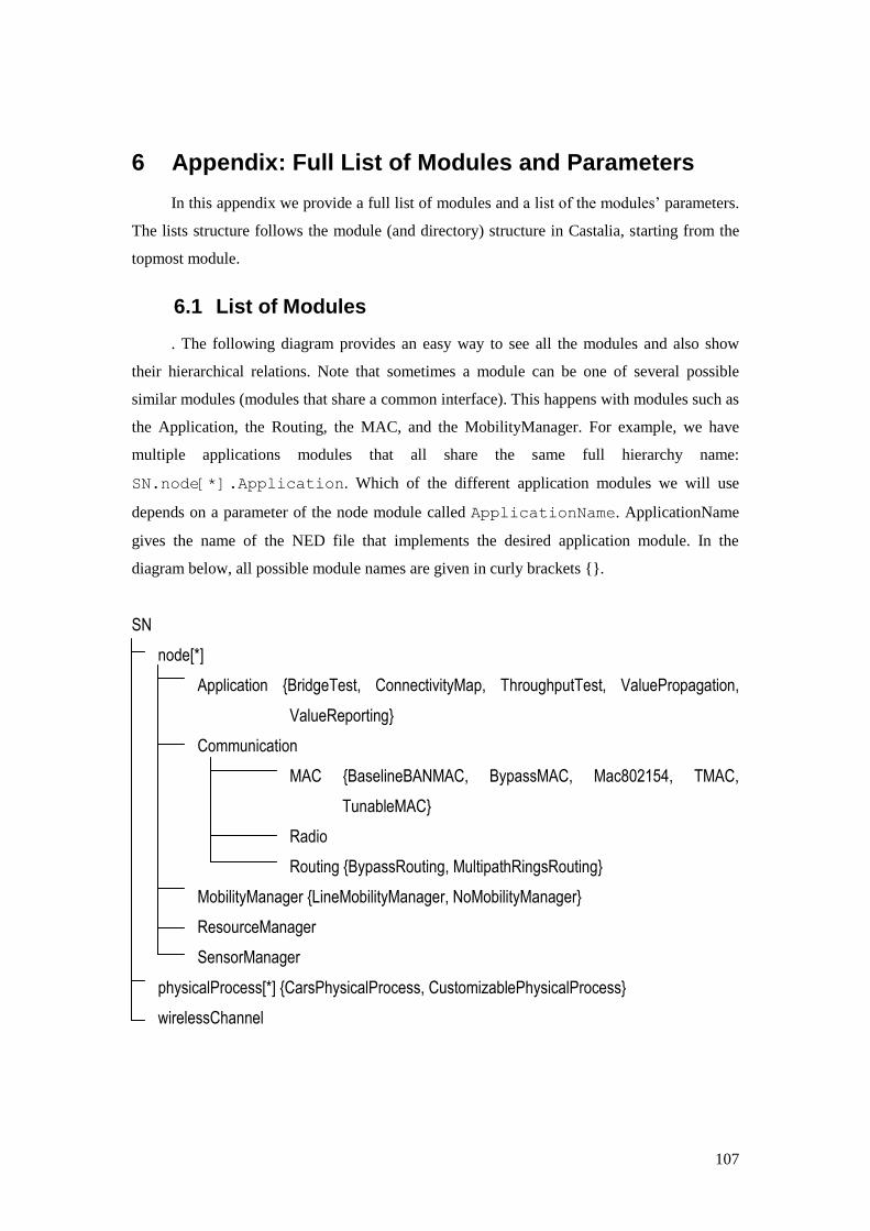
107
6 Appendix: Full List of Modules and Parameters
In this appendix we provide a full list of modules and a list of the modules‟ parameters.
The lists structure follows the module (and directory) structure in Castalia, starting from the
topmost module.
6.1 List of Modules
. The following diagram provides an easy way to see all the modules and also show
their hierarchical relations. Note that sometimes a module can be one of several possible
similar modules (modules that share a common interface). This happens with modules such as
the Application, the Routing, the MAC, and the MobilityManager. For example, we have
multiple applications modules that all share the same full hierarchy name:
SN.node[*].Application. Which of the different application modules we will use
depends on a parameter of the node module called ApplicationName. ApplicationName
gives the name of the NED file that implements the desired application module. In the
diagram below, all possible module names are given in curly brackets {}.
SN
node[*]
Application {BridgeTest, ConnectivityMap, ThroughputTest, ValuePropagation,
ValueReporting}
Communication
MAC {BaselineBANMAC, BypassMAC, Mac802154, TMAC,
TunableMAC}
Radio
Routing {BypassRouting, MultipathRingsRouting}
MobilityManager {LineMobilityManager, NoMobilityManager}
ResourceManager
SensorManager
physicalProcess[*] {CarsPhysicalProcess, CustomizablePhysicalProcess}
wirelessChannel

108
6.2 List of Parameters
The only generic OMNeT++ parameter that the user will be interested in setting is
sim-time-limit (or rarely cpu-time-limit, which limits the real cpu time of a
simulation). All the rest are Castalia-specific parameters. Parameters are listed per module.
First we give the NED file that describes the module and then we give the full hierarchy name
to reference the module. Parameters in the module have to be prefixed by the full hierarchy
name to be properly addressed in an .ini file. For example the Radio module has one
parameter called carrierFreq, and the full hierarchy name for the module is
SN.Node[*].Communication.Radio. Thus if we want to change the carrier frequency
of all the radios to 1000, the ini file has to include a line:
SN.Node[*].Communication.Radio.carrierFreq = 1000. Note the use of *
to access all radio modules in all nodes. Whenever there is an array of modules we will give
the full hierarchy name with a *, but the user is free to make it more specific based on
OMNeT++ syntax rules. Note also that some modules share the same full hierarchy name.
These are the modules found in curly brackets {} in the previous section. In the parameters
list you will see the notation “(shared)” next to the full hierarchy name to signify this.
Module NED file: src/SensorNework.ned
Full hierarchy name: SN
Parameter Name Default Value Refer
field_x 30 Section 3.2
field_y 30 Section 3.2
field_z 0 Section 3.2
numNodes Section 3.2
deployment Section 3.2
numPhysicalProcesses 1 Section 4.5
physicalProcessName “CustomizablePhysicalProcess” Section 4.5
debugInfoFileName “Castalia-Trace.txt” below
The debugIfoFileName is a string that gives the filename that all trace output will be written.
Module NED file: src/node/Node.ned
Full hierarchy name: SN.node[*]
Parameter Name Default Value Refer
xCoor 0 below

109
yCoor 0 below
zCoor 0 below
phi 0 below
theta 0 below
startupOffset 0 below
startupRandomization 0.05 below
ApplicationName Section 3.2
MobilityManagerName NoMobilityManager Section 3.2
xCoor, yCoor, zCoor, phi, theta give the initial position and initial orientation
of a node. Orientation is not currently being used to affect signal reception at the radio, or in
any way, but the parameters exist and are available to be used by applications if needed.
startupOffset is an absolute offset in seconds for the starting time of a node.
startupRandomization gives the upper bound of a time interval (in seconds). We draw
uniformly from that interval to affect the startup time of a node. Note that this randomly
drawn time is added to the offset.
Module NED file: src/node/application/bridgeTest/BridgeTest.ned
Full hierarchy name: SN.node[*].Application (shared)
Parameter Name Default Value Refer
applicationID “BridgeTest” Section 5.1
collectTraceInfo false Section 5.1
Priority 1 Section 5.1
packetHeaderOverhead 8 Section 5.1
constantDataPayload 0 Section 5.1
isSink 0 Section 3.6.2
reportDestination “0” Section 3.6.2
reportTreshold 10 Section 3.6.2
sampleInterval 100 Section 3.6.2
sampleSize 12 Section 3.6.2
reprogramInterval 86400 Section 3.6.2
reprogramPacketDelay 500 Section 3.6.2
reprogramPayload 5120 Section 3.6.2
maxPayloadPacketSize 128 Section 3.6.2

110
Module NED file: src/node/application/connectivityMap/ConnectivityMap.ned
Full hierarchy name: SN.node[*].Application (shared)
Parameter Name Default Value Refer
applicationID “connMap” Section 5.1
collectTraceInfo false Section 5.1
priority 1 Section 5.1
constantDataPayload 8 Section 5.1
packetSpacing 100 below
packetsPerNode 100 below
packetSize 32 below
PacketSpacing sets the interval between packet transmissions. packetsPerNode defines how
many packet will each node transmit, and packetsize is the packet size in bytes.
Module NED file: src/node/application/throughputTest/ThroughputTest.ned
Full hierarchy name: SN.node[*].Application (shared)
Parameter Name Default Value Refer
applicationID “throughputTest” Section 5.1
collectTraceInfo false Section 5.1
priority 1 Section 5.1
packetHeaderOverhead 5 Section 5.1
constantDataPayload 100 Section 5.1
nextRecipient “0” Section 5.1
packet_rate 0 below
startupDelay 0 below
latencyHistogramMax 200 below
latencyHistogramBuckets 10 below
The packet_rate sets the rate at which packets are transmitted by each node in packets/sec.
The startupDelay sets a delay in secs than the app will start transmitting after the node has
been activated. The latency histogram parameters set how the application level latency is to
be recorded
Module NED file: src/node/application/valuePropagation/ValuePropagation.ned
Full hierarchy name: SN.node[*].Application (shared)
Parameter Name Default Value Refer

111
applicationID “valuePropagation” Section 5.1
collectTraceInfo false Section 5.1
priority 1 Section 5.1
packetHeaderOverhead 8 Section 5.1
constantDataPayload 2 Section 5.1
tempThreshold 15.0 Section 3.5
Module NED file: src/node/application/valueReporting/ValueReporting.ned
Full hierarchy name: SN.node[*].Application (shared)
Parameter Name Default Value Refer
applicationID “valueReporting” Section 5.1
collectTraceInfo false Section 5.1
priority 1 Section 5.1
packetHeaderOverhead 8 Section 5.1
constantDataPayload 12 Section 5.1
maxSampleInterval 60000 below
minSampleInterval 1000 below
isSink false below
The max sample interval is used only to determine the effective sample interval of the app,
the min sample interval is not currently used. The isSink parameter shows which node(s) is
the sink.
Module NED file: src/node/communication/CommunicationModule.ned
Full hierarchy name: SN.node[*].Communication
Parameter Name Default Value Refer
MACProtocolName "BypassMAC" Section 3.2
RoutingProtocolName “BypassRouting” Section 3.2
Module NED file:
src/node/communication/mac/baselineBanMac/BaselineBANMac.ned
Full hierarchy name: SN.node[*].Communication.MAC (shared)
Parameter Name Default Value Refer
collectTraceInfo false Section 4

112
macMaxPacketSize 1000 Section 4.3.4
macBufferSize 32 Section 4.3.4
macPacketOverhead 7 Section 4.3.4
isHub false Section 4.3.4
allocationSlotLength 10 Section 4.3.4
beaconPeriodLength 32 Section 4.3.4
RAP1Length 8 Section 4.3.4
scheduledAccessLength 0 Section 4.3.4
scheduledAccessPeriod 1 Section 4.3.4
maxPacketTries 2 Section 4.3.4
contentionSlotLength 0.36 Section 4.3.4
enhanceGuardTime false Section 4.3.4
enhanceMoreData false Section 4.3.4
pollingEnabled false Section 4.3.4
naivePollingScheme false Section 4.3.4
pTIFS 0.03 Section 4.3.4
pTimeSleepToTX 0.2 Section 4.3.4
phyLayerOverhead 6 Section 4.3.4
phyDataRate Section 4.3.4
mClockAccuracy 0.0001 Section 4.3.4
Module NED file: src/node/communication/mac/bypassMac/BypassMAC.ned
Full hierarchy name: SN.node[*].Communication.MAC (shared)
Parameter Name Default Value Refer
collectTraceInfo false Section 4
macMaxPacketSize 0 below
macPacketOverhead 8 below
macBufferSize 0 below
These four parameter are standard for all MACs. macMaxPacketSize defines a limit to the
size of packets that the MAC can handle, macPacketOverhead gives you the overhead in
bytes added to the Network(routing) packets received from the layer above, and
macBufferSize is the size of the internal MAC buffer in packets.
Module NED file: src/node/communication/mac/mac802154/Mac802154.ned

113
Full hierarchy name: SN.node[*].Communication.MAC (shared)
Parameter Name Default Value Refer
collectTraceInfo false Section 4
printStateTransitions false Section 4.3.3
macMaxPacketSize 0 Section 4.3.3
macPacketOverhead 14 Section 4.3.3
macBufferSize 32 Section 4.3.3
enableSlottedCSMA true Section 4.3.3
enableCAP true Section 4.3.3
isFFD false Section 4.3.3
isPANCoordinator false Section 4.3.3
batteryLifeExtention false Section 4.3.3
frameOrder 4 Section 4.3.3
beaconOrder 6 Section 4.3.3
unitBackoffPeriod 20 Section 4.3.3
baseSlotDuration 60 Section 4.3.3
numSuperframeSlots 16 Section 4.3.3
macMinBE 5 Section 4.3.3
macMaxBE 7 Section 4.3.3
macMaxCSMABackoffs 4 Section 4.3.3
macMaxFrameRetries 2 Section 4.3.3
maxLostBeacons 4 Section 4.3.3
minCAPLength 440 Section 4.3.3
requestGTS 0 Section 4.3.3
phyDelayForValidCS 0.128 Section 4.3.3
phyDataRate Section 4.3.3
phyDelayRx2Tx 0.02 Section 4.3.3
phyFrameOverhead 6 Section 4.3.3
phyBitsPerSymbol Section 4.3.3
guardTime 1 Section 4.3.3
Module NED file: src/node/communication/mac/tMac/TMAC.ned
Full hierarchy name: SN.node[*].Communication.MAC (shared)
Parameter Name Default Value Refer
collectTraceInfo false Section 4

114
printStateTransitions false Section 4.3.2
ackPacketSize 11 Section 4.3.2
syncPacketSize 11 Section 4.3.2
rtsPacketSize 13 Section 4.3.2
ctsPacketSize 13 Section 4.3.2
macMaxPacketSize 0 Section 4.3.2
macPacketOverhead 11 Section 4.3.2
macBufferSize 32 Section 4.3.2
maxTxRetries 2 Section 4.3.2
allowSinkSync true Section 4.3.2
useFrts false Section 4.3.2
useRtsCts true Section 4.3.2
disableTAextension false Section 4.3.2
conservativeTA true Section 4.3.2
resyncTime 6 Section 4.3.2
contentionPeriod 10 Section 4.3.2
listenTimeout 15 Section 4.3.2
waitTimeout 5 Section 4.3.2
frameTime 610 Section 4.3.2
collisionResolution 0 Section 4.3.2
phyDelayForValidCS 0.128 Section 4.3.2
phyDataRate 250 Section 4.3.2
phyFrameOverhead 6 Section 4.3.2
Module NED file: src/node/communication/mac/tunableMac/tunableMAC.ned
Full hierarchy name: SN.node[*].Communication.MAC (shared)
Parameter Name Default Value Refer
collectTraceInfo false Section 4
printStateTransitions false
dutyCycle 1.0 Section 4.3.1
listenInterval 10 Section 4.3.1
beaconIntervalFraction 1.0 Section 4.3.1
probTx 1.0 Section 4.3.1
numTx 1 Section 4.3.1
randomTxOffset 0.0 Section 4.3.1

115
reTxInterval 0.0 Section 4.3.1
backoffType 1 Section 4.3.1
backoffBaseValue 16 Section 4.3.1
CSMApersistance 0 Section 4.3.1
txAllPacketsInFreeChannel true Section 4.3.1
sleepDuringBackoff false Section 4.3.1
macMaxPacketSize 0 Section 4.3.1
macPacketOverhead 9 Section 4.3.1
beaconFrameSize 14 Section 4.3.1
macBufferSize 32 Section 4.3.1
phyDataRate 250.0 Section 4.3.1
phyDelayForValidCS 0.128 Section 4.3.1
phyFrameOverhead 6 Section 4.3.1
Module NED file: src/node/communication/radio/Radio.ned
Full hierarchy name: SN.node[*].Communication.Radio (shared)
Parameter Name Default Value Refer
collectTraceInfo false Section 4
RadioParametersFile “” Section 4.2.1
mode “” Section 4.2.2
state “RX” Section 4.2.2
TxOutputPower “” Section 4.2.2
sleepLevel “” Section 4.2.2
carrierFreq 2400.0 Section 4.2.2
collisionModel 2 Section 4.2.2
CCAthreshold -95.0 Section 4.2.2
symbolsForRSSI 8 Section 4.2.2
carrierSenseInterruptEnabled false Section 4.2.2
bufferSize 16 Section 4.2.2
maxPhyFrameSize 1024 below
phyFrameOverhead 6 below
maxPhyFrameSize specifies the maximum length of a packet the radio can handle in bytes.
Some radios do pose restrictions on the size of packets they can handle so this parameter can
be useful modelling this behaviour. If set to 0 or less, it means we have no limit.

116
phyFrameOverhead specifies the overhead in bytes added to a packet received by the MAC
before being transmitted to the channel.
Module NED file:
src/node/communication/routing/bypassRouting/BypassRouting.ned
Full hierarchy name: SN.node[*].Communication.Routing (shared)
Parameter Name Default Value Refer
collectTraceInfo false Section 4
maxNetFrameSize 0 Section 4.4
netDataFrameOverhead 10 Section 4.4
netBufferSize 32 Section 4.4
Module NED file:
src/node/communication/routing/multipathRingsRouting/
MultipathRingsRouting.ned
Full hierarchy name: SN.node[*].Communication.Routing (shared)
Parameter Name Default Value Refer
collectTraceInfo false Section 4
maxNetFrameSize 0 Section 4.4
netBufferSize 32 Section 4.4
netDataFrameOverhead 14 Section 4.4
mpathRingsSetupFrameOverhead 13 Section 4.4
netSetupTimeout 50 Section 4.4
Module NED file: src/node/mobilityManager/LineMobilityManager.ned
Full hierarchy name: SN.node[*].MobilityManager (shared)
Parameter Name Default Value Refer
collectTraceInfo false Section 4
updateInterval 1000 Section 4.7
xCoorDestination 0 Section 4.7
yCoorDestination 0 Section 4.7
zCoorDestination 0 Section 4.7
speed 1 Section 4.7

117
Module NED file: src/node/mobilityManager/NoMobilityManager.ned
Full hierarchy name: SN.node[*].MobilityManager (shared)
Parameter Name Default Value Refer
collectTraceInfo false Section 4
Module NED file: src/node/resourceManager/ResourceManager.ned
Full hierarchy name: SN.node[*].ResourceManager
Parameter Name Default Value Refer
collectTraceInfo false Section 4
ramSize 0 Section 4.8
flashSize 0 Section 4.8
flashWriteCost 0 Section 4.8
flashReadCost 0 Section 4.8
imageSize 0 Section 4.8
cpuPowerSpeedLevelNames “” Section 4.8
cpuPowerPerLevel “” Section 4.8
cpuSpeedPerLevel “” Section 4.8
cpuInitialPowerLevel -1 Section 4.8
sigmaCPUClockDrift 0. 00003 Section 4.8
initialEnergy 18720 Section 4.8
baselineNodePower 6 Section 4.8
periodicEnergyCalculationInterval 1000 Section 4.8
Module NED file: src/node/sensorManager/SensorManager.ned
Full hierarchy name: SN.node[*].SensorManager
Parameter Name Default Value Refer
collectTraceInfo false Section 4
numSensingDevices 1 Section 4.6
pwrConsumptionPerDevice “0.02” Section 4.6
sensorTypes “Temperature” Section 4.6
corrPhyProcess “0” Section 4.6
maxSampleRates “1” Section 4.6
devicesBias “0.1” Section 4.6
devicesDrift “” Section 4.6

118
devicesNoise “0.1” Section 4.6
devicesHysterisis “” Section 4.6
devicesSensitivity “0” Section 4.6
devicesResolution "0.001" Section 4.6
devicesSaturation “1000” Section 4.6
Module NED file:
src/physicalProcess/carsPhysicalProcess/CarsPhysicalProcess.ned
Full hierarchy name: SN.physicalProcess[*] (shared)
Parameter Name Default Value Refer
collectTraceInfo false Section 4
max_num_cars 5 Section 4.5.2
car_speed 16.0 Section 4.5.2
car_value 30.0 Section 4.5.2
car_interarrival 20 Section 4.5.2
point1_x_coord Section 4.5.2
point2_x_coord Section 4.5.2
point1_y_coord Section 4.5.2
point2_y_coord Section 4.5.2
description “Moving cars” Section 4.5.2
Module NED file:
src/physicalProcess/customizablePhysicalProcess/CustomizablePhysic
alProcess.ned
Full hierarchy name: SN.physicalProcess[*] (shared)
Parameter Name Default Value Refer
collectTraceInfo false Section 4
inputType 1 Section 4.5.1
directNodeValueAssignment "(0)" Section 4.5.1
multiplicative_k 0.25 Section 4.5.1
attenuation_exp_a 1.0 Section 4.5.1
sigma 0.2 Section 4.5.1

119
max_num_snapshots 10 Section 4.5.1
numSources 1 Section 4.5.1
source_0 "0 10 10 30.5; 5 10 10 45; 12 10 10 7.3"
Section 4.5.1
source_1 “” Section 4.5.1
source_2 “” Section 4.5.1
source_3 “” Section 4.5.1
source_4 “” Section 4.5.1
tracefileName “” Section 4.5.1
description “Fire” Section 4.5.1
Module NED file: src/wirelessChannel/WirelessChannel.ned
Full hierarchy name: SN.wirelessChannel
Parameter Name Default Value Refer
collectTraceInfo false Section 4
onlyStaticNodes true Section 4.1.2
xCellSize 5 Section 4.1.2
yCellSize 5 Section 4.1.2
zCellSize 1 Section 4.1.2
pathLossExponent 2.4 Section 4.1.1
PLd0 55 Section 4.1.1
d0 1.0 Section 4.1.1
sigma 4.0 Section 4.1.1
bidirectionalSigma 1.0 Section 4.1.1
pathLossMapFile “” Section 4.1.1
temporalModelParametersFile “” Section 4.1.3
signalDeliveryThreshold -100 Section 4.1.4

120
7 References
[1] Draft Text Narrowband Physical Layer, https://mentor.ieee.org/802.15/dcn/10/15-10-
0195-02-0006-draft-text-narrowband-physical-layer.doc
[2] http://focus.ti.com/docs/prod/folders/print/cc1000.html
[3] http://focus.ti.com/docs/prod/folders/print/cc2420.html
[4] Marco Zuniga, Bhaskar Krishnamachari, "Analyzing the Transitional Region in Low
Power Wireless Links", First IEEE International Conference on Sensor and Ad hoc
Communications and Networks (SECON), Santa Clara, CA, October 2004.
[5] Karim Seada, Marco Zuniga, Ahmed Helmy, Bhaskar Krishnamachari, "Energy Efficient
Forwarding Strategies for Geographic Routing in Wireless Sensor Networks," ACM
Sensys 2004, November 2004.
[6] Yuri Tselishchev, Athanassios Boulis, Lavy Libman, “Experiences and Lessons from
Implementing a Wireless Sensor Network MAC Protocol in the Castalia Simulator,”
submitted to IEEE Wireless Communications & Networking Conference 2010 (WCNC
2010), Sydney, Australia.
[7] The IEEE 802.15.4 standard (ver. 2006)
http://standards.ieee.org/getieee802/download/802.15.4-2006.pdf
[8] MAC and Security Baseline Proposal, https://mentor.ieee.org/802.15/dcn/10/15-10-0196-
02-0006-mac-and-security-baseline-proposal-c-normative-text-doc.doc