ABSTRACT

Most of the research for wireless sensor networks has been done for terrestrial

applications. There is growing interest in marine wireless sensor networks for data

collection for oceanography applications, water conditions, and exploration. Marine

wireless sensor networks are in early stages of research and much work needs to be

done to move wireless sensor networks underwater. Currently, underwater nodes are

not available commercially making it hard to test existing protocols in an underwater

environment or develop new underwater protocols. This report presents a simulator

with underwater channel capabilities.

This project implements a simulator that contains an underwater acoustic chan-

nel. It is built on top of OMNeT++ and the MiXiM framework. The simulator

can run both underwater and terrestrial simulations. The simulator can use many of

MiXiM’s existing modules for MAC layer. The simulator provides a simple network-

ing layer that includes discovery, static clustering and simple routing. These modules

and MiXiM’s modules can be used as basis for developing new simulations.

A graphical user interface has been developed that can be used to configure and

run a simulation without using the OMNeT++ integrated development environment.

This interface is less complex, but allows most of the configuration parameters found

in OMNeT++ to be set. Configuration of specific nodes can be loaded through a

separate file.

ii

TABLE OF CONTENTS

Abstract . . . . . . . . . . . . . . . . . . . . . . . . . . . . . . . . . . . . ii

Table of Contents . . . . . . . . . . . . . . . . . . . . . . . . . . . . . . . iii

List of Figures . . . . . . . . . . . . . . . . . . . . . . . . . . . . . . . . vi

List of Tables . . . . . . . . . . . . . . . . . . . . . . . . . . . . . . . . . ix

1 Introduction . . . . . . . . . . . . . . . . . . . . . . . . . . . . . . . 1

1.1 Motivation . . . . . . . . . . . . . . . . . . . . . . . . . . . . . . 1

1.2 Discrete-Event Simulation . . . . . . . . . . . . . . . . . . . . . 2

2 Literature Review . . . . . . . . . . . . . . . . . . . . . . . . . . . . 4

2.1 Underwater Sensor Networks . . . . . . . . . . . . . . . . . . . . 4

2.1.1 Types of Underwater Sensor Networks . . . . . . . . . . . 4

2.1.2 Communication . . . . . . . . . . . . . . . . . . . . . . . 6

2.2 Existing Network Simulators . . . . . . . . . . . . . . . . . . . . 7

2.2.1 ns2 . . . . . . . . . . . . . . . . . . . . . . . . . . . . . . 7

2.2.2 ns3 . . . . . . . . . . . . . . . . . . . . . . . . . . . . . . 9

2.2.3 OPNET Modeller . . . . . . . . . . . . . . . . . . . . . . 9

2.2.4 OMNeT++ . . . . . . . . . . . . . . . . . . . . . . . . . . 10

2.3 Wireless Sensor Network Simulators . . . . . . . . . . . . . . . . 11

2.3.1 Sensim . . . . . . . . . . . . . . . . . . . . . . . . . . . . 11

2.3.2 Castalia . . . . . . . . . . . . . . . . . . . . . . . . . . . . 12

2.3.3 SENSE . . . . . . . . . . . . . . . . . . . . . . . . . . . . 13

2.3.4 Aqua-Sim . . . . . . . . . . . . . . . . . . . . . . . . . . . 14

iii

3 Underwater Acoustic WSN Simulator . . . . . . . . . . . . . . . . . 15

3.1 Requirements . . . . . . . . . . . . . . . . . . . . . . . . . . . . 15

3.1.1 Structured Requirements . . . . . . . . . . . . . . . . . . 18

3.2 Design . . . . . . . . . . . . . . . . . . . . . . . . . . . . . . . . 21

3.2.1 User Interface . . . . . . . . . . . . . . . . . . . . . . . . 22

3.2.2 Logging . . . . . . . . . . . . . . . . . . . . . . . . . . . . 22

3.2.3 Visualize Simulation . . . . . . . . . . . . . . . . . . . . . 22

3.2.4 Add Algorithm . . . . . . . . . . . . . . . . . . . . . . . . 23

3.3 Implementation . . . . . . . . . . . . . . . . . . . . . . . . . . . 24

3.3.1 The MiXiM Model . . . . . . . . . . . . . . . . . . . . . . 24

3.3.2 Underwater Acoustic Channel . . . . . . . . . . . . . . . 27

3.3.3 Simple Protocols . . . . . . . . . . . . . . . . . . . . . . . 32

3.4 UASim GUI . . . . . . . . . . . . . . . . . . . . . . . . . . . . . 34

3.4.1 Configuration Files . . . . . . . . . . . . . . . . . . . . . 35

3.4.2 Classes . . . . . . . . . . . . . . . . . . . . . . . . . . . . 37

3.5 Evaluation and Results . . . . . . . . . . . . . . . . . . . . . . . 42

3.5.1 Sample Simulation Runs . . . . . . . . . . . . . . . . . . 43

3.5.2 Known Issues . . . . . . . . . . . . . . . . . . . . . . . . . 46

4 Conclusions and Future Work . . . . . . . . . . . . . . . . . . . . . 50

4.1 Future Work . . . . . . . . . . . . . . . . . . . . . . . . . . . . . 51

Dedication . . . . . . . . . . . . . . . . . . . . . . . . . . . . . . . . . . . . . 52

iv

Acknowledgments . . . . . . . . . . . . . . . . . . . . . . . . . . . . . . . . . 53

Bibliography and References . . . . . . . . . . . . . . . . . . . . . . . . . . . 54

Appendix A. Use Case Textual Descriptions . . . . . . . . . . . . . . . . . . . 56

A.2 High-level Use Case . . . . . . . . . . . . . . . . . . . . . . . . . 56

A.2.1 Configure Simulation . . . . . . . . . . . . . . . . . . . . 56

A.2.2 Run Simulation . . . . . . . . . . . . . . . . . . . . . . . 56

A.2.3 Visualize Simulation . . . . . . . . . . . . . . . . . . . . . 57

A.2.4 Add Algorithm . . . . . . . . . . . . . . . . . . . . . . . . 57

A.3 Configure Simulation Use Case . . . . . . . . . . . . . . . . . . . 58

A.3.1 Set Simulation Parameters . . . . . . . . . . . . . . . . . 58

A.3.2 Set Module Parameters . . . . . . . . . . . . . . . . . . . 58

A.3.3 Load Node Data . . . . . . . . . . . . . . . . . . . . . . . 59

A.3.4 Reset To Defaults . . . . . . . . . . . . . . . . . . . . . . 60

A.4 Add Algorithm Use Case . . . . . . . . . . . . . . . . . . . . . . 60

A.4.1 Develop Module . . . . . . . . . . . . . . . . . . . . . . . 60

A.4.2 Create Parameter Configuration File . . . . . . . . . . . . 60

A.4.3 Add Module To GUI Configuration . . . . . . . . . . . . 61

Appendix B. User’s Guide . . . . . . . . . . . . . . . . . . . . . . . . . . . . 62

B.1 Installation . . . . . . . . . . . . . . . . . . . . . . . . . . . . . . 62

B.1.1 OMNeT++ . . . . . . . . . . . . . . . . . . . . . . . . . . 62

B.1.2 MiXiM . . . . . . . . . . . . . . . . . . . . . . . . . . . . 62

v

B.1.3 UASim . . . . . . . . . . . . . . . . . . . . . . . . . . . . 62

B.2 Using UASim . . . . . . . . . . . . . . . . . . . . . . . . . . . . 67

B.2.1 The General Tab . . . . . . . . . . . . . . . . . . . . . . . 67

B.2.2 Other Configuration Tabs . . . . . . . . . . . . . . . . . . 67

B.2.3 Loading Node Data . . . . . . . . . . . . . . . . . . . . . 67

B.2.4 Running A Simulation . . . . . . . . . . . . . . . . . . . . 68

B.2.5 Results . . . . . . . . . . . . . . . . . . . . . . . . . . . . 69

Appendix C. Programmer’s Guide . . . . . . . . . . . . . . . . . . . . . . . . 70

C.1 Required Tools . . . . . . . . . . . . . . . . . . . . . . . . . . . . 70

C.1.1 Packages needed for GUI Development . . . . . . . . . . . 70

C.2 Adding to the Simulation Engine . . . . . . . . . . . . . . . . . 71

C.3 Modifications to the GUI . . . . . . . . . . . . . . . . . . . . . . 71

vi

LIST OF FIGURES

1.1 Discrete event simulation components. . . . . . . . . . . . . . . . . . 3

2.1 2D architecture . . . . . . . . . . . . . . . . . . . . . . . . . . . . . . 5

2.2 3D architecture . . . . . . . . . . . . . . . . . . . . . . . . . . . . . . 6

2.3 Model structure in OMNeT++ . . . . . . . . . . . . . . . . . . . . . 11

2.4 Basic structure of a sensor node in Sensim . . . . . . . . . . . . . . . 12

2.5 Basic module structure in Castalia . . . . . . . . . . . . . . . . . . . 13

2.6 Castalia node . . . . . . . . . . . . . . . . . . . . . . . . . . . . . . . 14

3.1 High level use case diagram for simulator. . . . . . . . . . . . . . . . 16

3.2 Configure Simulation use case diagram. . . . . . . . . . . . . . . . . . 17

3.3 Add Algorithm use case diagram. . . . . . . . . . . . . . . . . . . . . 17

3.4 UASim block diagram. . . . . . . . . . . . . . . . . . . . . . . . . . . 21

3.5 Possible screens for user interface. . . . . . . . . . . . . . . . . . . . . 23

3.6 Basic MiXiM simulation. . . . . . . . . . . . . . . . . . . . . . . . . . 24

3.7 MiXiM basic node and NIC modules. . . . . . . . . . . . . . . . . . . 25

3.8 Classes in MiXiM. . . . . . . . . . . . . . . . . . . . . . . . . . . . . 26

3.9 Class diagram of MiXiM physical layer . . . . . . . . . . . . . . . . . 29

3.10 filterSignal method from SeaWater . . . . . . . . . . . . . . . . . . . 32

3.11 findCluster method from OurBaseNet . . . . . . . . . . . . . . . . . . 33

3.12 findRoute method from OurBaseNet . . . . . . . . . . . . . . . . . . . 34

3.13 uasim.xml. . . . . . . . . . . . . . . . . . . . . . . . . . . . . . . . . 36

vii

3.14 An all.xml. . . . . . . . . . . . . . . . . . . . . . . . . . . . . . . . . 36

3.15 A configuration file for a UASim module. . . . . . . . . . . . . . . . 37

3.16 A per node configuration file. . . . . . . . . . . . . . . . . . . . . . . 37

3.17 Class diagram of UASim . . . . . . . . . . . . . . . . . . . . . . . . . 38

3.18 Code to get module parameters from the panel. . . . . . . . . . . . . 39

3.19 General configuration tab of UASim. . . . . . . . . . . . . . . . . . . 40

3.20 A configuration panel in UASim. . . . . . . . . . . . . . . . . . . . . 41

3.21 The configuration display window. . . . . . . . . . . . . . . . . . . . 42

3.22 Difference in connectivity. . . . . . . . . . . . . . . . . . . . . . . . . 44

3.23 Simulation with one cluster. . . . . . . . . . . . . . . . . . . . . . . . 45

3.24 A simulation with four clusters and eight nodes. . . . . . . . . . . . . 46

3.25 Screen shots from UASim. . . . . . . . . . . . . . . . . . . . . . . . . 47

3.26 The display of simulation parameters prior to running simulation. . . 48

3.27 Output from OMNeT++ that shows the connect manager used. . . . 48

3.28 OMNeT++ simulation screen. . . . . . . . . . . . . . . . . . . . . . . 48

3.29 A screen shot of the simulation running. . . . . . . . . . . . . . . . . 49

3.30 End of simulation dialog. . . . . . . . . . . . . . . . . . . . . . . . . 49

B.1 OMNeT++ installion. . . . . . . . . . . . . . . . . . . . . . . . . . . 64

B.2 Install UASim into OMNeT++ . . . . . . . . . . . . . . . . . . . . . 65

B.3 Install UASim into OMNeT++ . . . . . . . . . . . . . . . . . . . . . 66

B.4 UASim configuration tabs. . . . . . . . . . . . . . . . . . . . . . . . . 68

B.5 A per node configuration file. . . . . . . . . . . . . . . . . . . . . . . 68

viii

B.6 Buttons to start visual simulation run. . . . . . . . . . . . . . . . . . 69

C.1 uasim.xml. . . . . . . . . . . . . . . . . . . . . . . . . . . . . . . . . 72

C.2 An all.xml. . . . . . . . . . . . . . . . . . . . . . . . . . . . . . . . . 72

C.3 A configuration file for a UASim module. . . . . . . . . . . . . . . . 73

ix

LIST OF TABLES

TABLE Page

3.1 System requirements . . . . . . . . . . . . . . . . . . . . . . . . . . . 16

x

1. INTRODUCTION

Simulation is the imitation of something real, used to test and study real-life or to

practice skills or tasks when practice in the real-world is not viable due to cost or safety

issues. Simulation for computer scientists involves modeling real-life or hypothetical

situations on a computer. Network simulators model devices and traffic in a computer

network. They are used to test new protocols, study how different protocols interact

or analyze performance.

Wireless Sensor Networks (WSN) are made up of tiny sensors that are generally

used to sense their environment. WSN are usually infrastructureless networks that

rely on each sensor to function as part of the network. Each WSN is application

specific, so no standard protocols like Ethernet or TCP have emerged. Most of the

research for WSN has been for terrestrial environments. There is growing interest in

marine WSN for collection of data for oceanography applications, water conditions,

and exploration. Because of current lack of underwater wireless sensors, development

of necessary protocols for marine WSN will benefit from a simulator designed to deal

with underwater conditions.

1.1 Motivation

It appears that commonly used protocols in terrestrial WSN will not be as effective

underwater so research is needed to create new protocols or modify existing ones

[1]. This is because of the underwater channel and its effects on the signals used

in communication. Also power consumption is a concern with marine WSN. The

protocols used in marine WSN will need to be low-energy protocols developed for the

underwater environment.

Underwater nodes are not commercially available at this time, making it very

costly to develop a test-bed for marine WSN. This makes it difficult to test or evaluate

1

the performance of existing and proposed algorithms in an underwater setting. A

simulator that can handle marine conditions would be beneficial for researchers. This

simulator can be used to evaluate the performance of algorithms without building a

test-bed.

The TAMUCC WSN group requires a simulator that they can use to test pro-

posed protocols. They require a system that allows them to build, run, and visualize

simulations. It needs to have an underwater channel. They need to be able to extend

the system and it needs to run under Microsoft WindowsTM operating system. While

there are many simulators for wired and wireless networks including WSN, only one

has been found for marine WSN (Section 2.3.4) and it does not meet all of the re-

quirements of the TAMUCC WSN group, namely the ability to run on a Microsoft

WindowsTM operating system. There is concern about it being based on ns2 (Section

2.2.1) since it is being replaced with ns3 (Section 2.2.2) and ns3 is not backwards

compatible with ns2.

1.2 Discrete-Event Simulation

Most of the network simulators available today are discrete-event simulators. Discrete-

event simulations can be viewed as the flow of traffic or transactions in the system[2].

Each discrete piece of traffic flows from point to point and may have to compete for

utilization of resources with other traffic. A discrete-event simulation is one where

the model changes only at a discrete set of time points. These time points are often

randomly chosen. Simultaneously occurring events are done serially within the time

point.

Within a simulation there exists an entity (traffic or transaction) that instigates

and responds to events. Events are happenings that change the state of the model.

Entities can be external (specified by the modeller) or internal (created by the sim-

2

ulation software). A resource is a system element that provides a service. Entities

typically use resources. Resources may be limited and entities have to compete for

them or wait for them to be available. A control element deals with system state. An

operation is something an entity does or happens to it. An example of components

in a discrete-event simulation is customers queueing for bank tellers. Customers are

entities which wait for resources, the bank tellers. Events happen when customers

enter the queue, leave the queue or leave the teller. Operations would be actions

performed by the customer, like depositing money. Figure 1.1 shows customers at the

bank.

Fig. 1.1. Discrete event simulation components. Customers are entities. Tellers are

resources. Events happen when customers enter queue, leave queue, and

leave teller. Operations like deposit money are performed by customers.

3

2. LITERATURE REVIEW

In this section introduces underwater wireless sensor networks and how they are

currently being used. Then some existing networking simulators are reviewed.

2.1 Underwater Sensor Networks

Underwater Sensor Networks (USN) are used to monitor different conditions un-

derwater including temperature, pressure and salinity. Some USN include wireless

communications and some do not. Marine or underwater WSN are in early stages of

research and many ideas about node architecture, network architecture and protocols

are only theoretical.

2.1.1 Types of Underwater Sensor Networks

This section introduces some actual and proposed USN.

Sensor Retrieval

In some USN, sensors include some limited storage capacity and their collected

data is saved to that storage. The sensors are gathered from the water when data

collection is finished and the data is retrieved from the sensor [3]. No underwater

communication is involved.

Wired/Wireless Mix

In this type of USN [4], the sensors are attached to a buoy with a wire. They

communicate their sensed data over the wire. The buoys have some wireless commu-

nication capability that is used to communicate with other buoys and the shore.

2D Architecture

A proposed architecture [3] for Marine WSN, called a 2D architecture, has the

sensors anchored to the seabed. Sensors then communicate wirelessly to an under-

4

water sink. The underwater sink is responsible for communications with a surface

station. The surface station communicates with mobile sinks and the shore. Figure

2.1 shows a 2D architecture.

Fig. 2.1. 2D Architecture [3].

3D Architecture

The 3D architecture [3] is similar to the 2D architecture except the sensors are

anchored at different levels to take readings throughout the water column. The

underwater sink is removed and the sensors communication multi-hop to the surface

station. Figure 2.2 shows a 3D architecture.

Data Retrieval Using An Autonomous Underwater Vehicle

In this type of system [5, 6, 7, 8] sensors are place on the seabed. Each sensor

has some limited storage capacity that it uses to save sensed data. An Autonomous

Underwater Vehicle (AUV) travels through the water and collects data from each

sensor using wireless communications. The AUV then returns to the surface with the

retrieved data.

5

Fig. 2.2. 3D Architecture [3].

Another use of an AUV is to equip it with sensors and have it collect data as it

moves through water. They can function without tethers, cables, or remote control,

making them a good choice for many applications in oceanography, environment

monitoring, and resource study [3].

Smart Plankton

The Smart Plankton project [9, 10] proposes to develop nodes for marine WSN

based on marine biology and aquatic micro-organisms. Smart Plankton aren’t an-

chored to seabed, but drift in the water column like real plankton.

2.1.2 Communication

Radio Frequency (RF) which is used in terrestrial WSN is not the medium typ-

ically used when doing wireless communications underwater. The high frequency

radio waves are strongly attenuated in water making them unsuitable for underwater

communication.

6

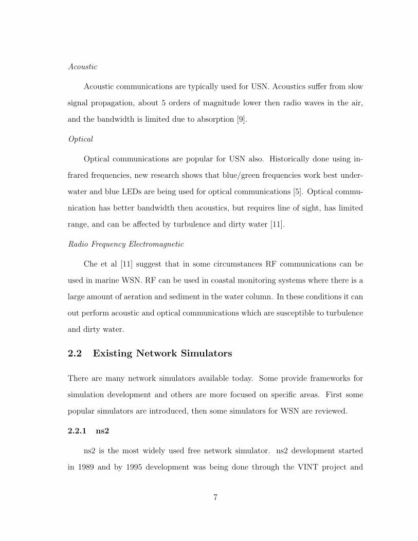
Acoustic

Acoustic communications are typically used for USN. Acoustics suffer from slow

signal propagation, about 5 orders of magnitude lower then radio waves in the air,

and the bandwidth is limited due to absorption [9].

Optical

Optical communications are popular for USN also. Historically done using in-

frared frequencies, new research shows that blue/green frequencies work best under-

water and blue LEDs are being used for optical communications [5]. Optical commu-

nication has better bandwidth then acoustics, but requires line of sight, has limited

range, and can be affected by turbulence and dirty water [11].

Radio Frequency Electromagnetic

Che et al [11] suggest that in some circumstances RF communications can be

used in marine WSN. RF can be used in coastal monitoring systems where there is a

large amount of aeration and sediment in the water column. In these conditions it can

out perform acoustic and optical communications which are susceptible to turbulence

and dirty water.

2.2 Existing Network Simulators

There are many network simulators available today. Some provide frameworks for

simulation development and others are more focused on specific areas. First some

popular simulators are introduced, then some simulators for WSN are reviewed.

2.2.1 ns2

ns2 is the most widely used free network simulator. ns2 development started

in 1989 and by 1995 development was being done through the VINT project and

7

supported by DARPA [12]. ns2 was to provide an improved set of tools for researchers

to simulate networks[13]. The developers concluded that researchers would benefit

from a common, well tested simulation environment. This would provide researchers

with a common format for results allowing for easier comparison across research

endeavors and validated models for common protocols. A well built simulator would

also provide a way to study protocol interaction. With better tools, researchers can

spend their time developing protocols instead of developing simulators for individual

work.

There are five capabilities that were important to ns2 development: abstraction,

emulation, scenario generation, visualization, and extensibility [13].

• Abstraction allows for detail hiding. When studying a protocol at a low level,

the details are important. Observing protocol interaction may not require a high

level of detail and the detail can be abstracted out giving better performance in

the simulation. Higher abstraction means less accuracy in the simulation, but

in many scenarios this may be acceptable.

• Emulation is when the simulator is connected to a live network and traffic flows

between the simulator and real-world network nodes.

• Scenario generation assists with building appropriate test scenarios especially

in large simulations. Scenario generations handles topology, traffic patterns

and dynamic events such as link failures. ns2 provides an interface to load

topologies from other programs designed specifically for topology generation.

New programs can be used usually with just a conversion of file format. The

ns2 library contains modules to simulate different traffic patterns such as web

or ftp traffic.

8

• Visualization of simulation data and results assists researchers in understanding

the behavior of the network.

• Easy extensibility allows users to add new protocols, functionality, and scenar-

ios.

ns2 has a split programming model. Protocols are implemented in C++. Topol-

ogy and scenario description are done in an object-oriented version of Tcl called oTcl.

This design is used to make protocols more efficient and the scripts that control the

simulation easy to write.

2.2.2 ns3

ns3 [14] is the eventual replacement of ns2. It is a combination of all patches to

ns2 and some enhancements. ns3 tries to avoid some of the problems in ns2 like inter-

operability and coupling between models, lack of memory management, debugging of

split language objects. Because of some of the design decisions, ns3 is not backward

compatible with ns2. The collection of protocols available in ns2 has to be ported to

ns3. The split programming environment is now optional. All modelling can be done

purely in C++ or scripting can be done with Python.

2.2.3 OPNET Modeller

OPNET Modeler[15] is a full-featured commercial product produced by OPNET

Technologies. It is the fastest discrete event simulator in industry[15]. It contains

hundreds of models for wired/wireless protocols and vendor devices. OPNET Modeler

provides a GUI-based debugging and analysis environment. The simulator is free to

qualified universities. OPNET Modeler contains an add-on for wireless networks.

9

2.2.4 OMNeT++

Objective Modular Network Test-bed in C++ (OMNeT++)[16] is a generic

framework for discrete-event simulation. While it was designed for network simu-

lation, it is also used in other areas. It is intended to fill the gap between ns2 and

expensive commercial products like OPNET. OMNeT++ provides basic tools to build

simulations. OMNeT++ design requirements include:

• Simulation models should be hierarchical and built from reusable components.

This allows for large-scale simulation.

• Simulation software should aid in visualization and debugging of the simulation

model.

• The simulation engine should be modular and allow for customization.

• Simulations should be embeddable in larger applications.

• Data interfaces should be open.

• Simulation software should provide an Integrated Development Environment

(IDE) for development of simulations and analysing results.

Frameworks that assist with simulation of networks have been developed using

OMNeT++. These include a comprehensive collection of Internet protocol models

in the INET Framework and the Mobility Framework which contains wireless sensor

network simulation modules. These are developed independently of OMNeT++.

An OMNeT++ model is built using modules that communicate by message pass-

ing. Simple modules are the lowest level and are developed in C++. They can be

grouped together to form compound modules. There is not a limit to the number of

levels in the hierarchy. The module structure is shown in Figure 2.3.

10

Fig. 2.3. Model structure in OMNeT++. Heavy lines show simple modules. Thin

lines show compound modules.[16]

Simple modules are built using OMNeT++’s object library. This library includes

functionality for high-level debugging and tracing capabilities.

The structure of the model is written in NED, OMNeT++’s topology description

language. Model behavior is found in the C++ code. Model topology is included in

the NED files. Other simulation data, like inputs that may vary from run to run, is

kept in INI files. This separation of information keeps the model clean and allows for

better tooling support.

2.3 Wireless Sensor Network Simulators

The focus on simulators for WSN seems to be on providing a sensor model that can

be modified to suit a researcher’s needs and a way to connect the nodes together to

form a network. The following sections introduce some simulators for WSN. With

the exception of Aqua-Sim in Section 2.3.4 none of these simulators support marine

WSN.

2.3.1 Sensim

Sensim[17] is a general purpose simulator for WSN built on top of OMNeT++,

meant to be similar to the Mobility Framework for OMNeT++ . Sensim implements

each layer of a node as a simple module. The node itself is a compound module

11

that contains the layer modules, hardware modules, and a CoOrdinator module. The

CoOrdinator module coordinates the activities of the hardware and the software mod-

ules. For example, the Battery module will be updated when a message is sent in the

Physical Layer module to reflect the amount of battery used. Figure 2.4 shows the

structure of a node.

Fig. 2.4. Basic structure of a sensor node in Sensim.[17]

MAC 802.11 (MAC Layer) and Directed Diffusion with Geographical and En-

ergy Aware routing (Network Layer) have been implemented using Sensim’s design.

Studies of the simulator have shown it to be an order of magnitude faster then ns2

and it has more efficient memory usage.

2.3.2 Castalia

Castalia[18] is another WSN simulator built on top of OMNeT++. Its focus

is to provide realistic models for the radio and wireless channel. It strives for real-

12

istic node behavior in relation to access of the radio and handles clock drift in the

node. The channel module is based on empirically measured data. The radio model

captures features of real low-power radios including multiple states and transmission

power levels. Figure 2.5 shows the basic module structure of Castalia. Each node

is connected to one or more wireless channels and one or more physical processes.

Since a node might communicate on different frequencies there are multiple wireless

channels. Multiple physical processes are provided if the node has multiple sensors.

Fig. 2.5. Basic module structure in Castalia.[18]

The structure of a node is shown in Figure 2.6. A Castalia node contains simple

modules for sensors, application layer and hardware resources. Communications to

the wireless channel is a compound module that consists of models for routing, MAC

and radio.

2.3.3 SENSE

SENSE [19] is a simulator for WSN developed on top of a discrete-event simulator

called COST. SENSE is component-oriented architecture designed to avoid the inter-

13

Fig. 2.6. Castalia node.[18]

dependency of modules often found with object-oriented design. Their component-

port model allows for a new component to replace any existing one as long as interfaces

do not change. SENSE aims to be extensible, reusable and scalable. It provides bat-

tery, application, network, MAC and physical layer models, wireless channel and a

sequential simulation engine.

2.3.4 Aqua-Sim

Aqua-Sim is a simulator for underwater sensor networks [20]. It is built on top

of ns2. It is intended to be run in parallel with the CMU wireless package [21].

Aqua-Sim is the only simulator that we have found that is designed for marine WSN.

It implements an acoustic channel, handling attenuation and collisions in a manner

appropriate for underwater conditions. The simulator has been tested against the

test-bed at University of Connecticut’s Underwater Sensor Network Lab. The tests

show that Aqua-Sim can reliably simulate the real world [22].

14

3. UNDERWATER ACOUSTIC WSN SIMULATOR

This section discusses the requirements, design, and implementation of this project’s

underwater acoustic WSN simulator, UASim. Some results from the simulator are

also provided.

3.1 Requirements

This project proposes a simulator that focuses on marine WSN. The simulator will be

able to handle terrestrial WSN networks in addition to marine WSN. The primary use

of the simulator is to test proof of concept for MAC and networking protocols. It needs

to have a modular design to make it easy to “plug and play” different combinations

of protocols. Users should have some mechanism to add new protocols. Since the

simulator needs to simulate marine WSN, development of a model for an acoustic

channel is required.

The simulator should provide a graphical user interface that allows the user

to configure a simulation run, actually run the simulation and then visualize the

results. The system needs to be able to scale to a large amount of sensor nodes. A

set of core protocols should be provided with the simulator. These protocols should

include common MAC protocols, routing protocols and protocols to handle clustering.

Both static and dynamic clustering protocols are required. Table 3.1 shows lists of

functional and non-functional requirements.

Configuration options should include type of network, number of nodes, proto-

col/algorithms to use, clustering options, and number of runs. Figures 3.1, 3.2 and

3.3 show the use case diagrams for the marine WSN simulator. Appendix A contains

the textual descriptions for the use cases.

15

Requirements

Non-functional Functional

Scalable Configure simulation

Extensible Visualize simulation and results

Modular Provide core protocols

Run under Windows Model underwater wireless channel

Graphical user interface Add algorithms to system

Table 3.1. System requirements

Fig. 3.1. High level use case diagram for simulator.

16

Fig. 3.2. Configure Simulation use case diagram.

Fig. 3.3. Add Algorithm use case diagram.

17

3.1.1 Structured Requirements

Configure Simulation

1. The interface should allow the user to configure simulations

(a) The system displays the General tab with default configuration values

(b) The user selects the network type

(c) The user enters general simulation parameters

(d) The user indicates if she wants a visual of the simulation

(e) The user can enter more configuration parameters

i. The user selects a tab

ii. The system switches to the selected tab

iii. The user enters desired options

(f) The user can reset to default configuration parameters

i. The user clicks on “Reset To Defaults” button

ii. The system resets all configuration values to the default values

(g) The user can load per node configuration parameters

i. The user clicks on “File” menu

ii. The system displays the “File” menu

iii. The user selects “Load Nodes” option

iv. The system displays a file chooser

v. The user selects the desired file and presses “Open”

vi. The system closes the file chooser

vii. The system reads the per node configuration from the selected file

18

viii. The user is viewing the last selected configuration tab

(h) The user presses the “OK” button when all options are entered

(i) The system displays a window containing the configuration parameters

and their current values

Run Simulation

1. The interface should allow the user to run a simulation

(a) The user configures the simulation and presses “OK”

(b) The system displays a window containing the configuration parameters

and their current values

(c) The user presses the “Run” button

(d) The system writes out necessary configuration files

(e) The system runs the simulation

(f) The system displays a visual of the simulation if requested

(g) The system indicates that the simulation is running with a busy cursor

(h) The system detects when the simulation is done

(i) The system changes to the regular cursor

(j) The user is viewing the last selected configuration tab

Visualize Simulation Results

1. The user should be able to visualize simulation results

(a) The user runs the OMNeT++ IDE

(b) The user opens the “runsim” project

19

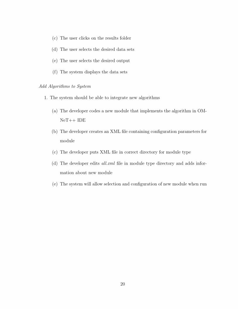
(c) The user clicks on the results folder

(d) The user selects the desired data sets

(e) The user selects the desired output

(f) The system displays the data sets

Add Algorithms to System

1. The system should be able to integrate new algorithms

(a) The developer codes a new module that implements the algorithm in OM-

NeT++ IDE

(b) The developer creates an XML file containing configuration parameters for

module

(c) The developer puts XML file in correct directory for module type

(d) The developer edits all.xml file in module type directory and adds infor-

mation about new module

(e) The system will allow selection and configuration of new module when run

20

3.2 Design

OMNeT++ is an extensible, modular, component-based C++ simulation library and

framework, with an Eclipse-based Integrated Development Environment (IDE) and a

graphical runtime environment [23]. It is free for academic use. OMNeT++ provides

a discrete event simulation engine, graphical and command-line execution of simula-

tions, and visualization of results eliminating the need to develop these pieces. MiXiM

[24] is a framework for wireless and mobile networks developed using OMNeT++. It

contains base models for physical, network, and MAC layers that can be used to build

the functionality of wireless nodes. This project will be using OMNeT++ and MiXiM

as the framework for our marine WSN simulator. Figure 3.4 shows a block diagram

of the system.

Fig. 3.4. UASim block diagram.

An “expert” user can choose to build/run simulations using only the OMNeT++

IDE. She will be able to build simulations using modules from any of OMNeT++

21

model frameworks and the components developed specifically for this project based

on MiXiM. Other users may choose a simpler interface developed with this project

that will be used in place of the OMNeT++ IDE for simulation configuration and

execution. This interface will generate configuration and NED files needed to run

simulations and run simulations with either OMNeT++’s command-line or visual

interface. Both users will use the OMNeT++ IDE for visualization of results. Other

visualization options will be developed if needed.

3.2.1 User Interface

OMNeT++ uses several configuration files and NED files to define a simulation.

To simplify the configuration of a simulation run, a Graphical User Interface (GUI)

will be developed to generate needed configuration files for OMNeT++. Figure 3.5

shows possible screens for the user interface. The interface will allow for the user to

run the simulation.

3.2.2 Logging

As the simulation runs, certain metrics will be logged. OMNeT++ allows vector

and scalar output from modules. This data is collected by the different modules.

Modules may need to be configured or modified to get saved data. The data is

written to text files that can be processed by the Analysis Tool in the IDE. They can

also be processed by other tools. There is also an event log that captures detailed

information of the simulation that can be used to verify that modules are running as

expected.

3.2.3 Visualize Simulation

The OMNeT++ IDE will be used to visualize the simulation results. If necessary,

additional tools will be written to aid with simulations results.

22

(a) General tab. (b) Clustering tab.

(c) Protocol tab. (d) Node tab.

Fig. 3.5. Possible screens for user interface.

3.2.4 Add Algorithm

To add an algorithm, the user will need to develop an OMNeT++ module that

implements the functionality of the new algorithm. This will be written in C++. A

new algorithm module is added to the configuration files for the developed GUI. This

allows the new algorithm to be available to the end user.

23

3.3 Implementation

This section discusses MiXiM’s wireless model and describes how the simulator was

implemented.

3.3.1 The MiXiM Model

MiXiM provides a structure for nodes and a means to connect them together

for communications. Figure 3.6 shows a basic MiXiM simulation. It is made up of

a number of nodes, a connection manager, world utility module, and the playground

(the region where nodes can be placed). The world utility module stores global

information about the simulation like the size of the playground. The connection

manager is responsible for setting up the communications between the nodes.

Fig. 3.6. Basic MiXiM simulation.

Figure 3.7 shows the structure of a node in MiXiM. Each node is comprised

of modules that represent networking layers and other functionality of a node like

mobility. Each node contains a module for the application, networking layer, and

NIC. The NIC is composed of two modules, the MAC layer and physical layer. These

modules communicate primarily through message passing that is implemented to

closely represent the functionality of the network stack. Base functionality is provided

24

(a) Basic node. (b) Basic NIC.

Fig. 3.7. MiXiM basic node and NIC modules.

in each module that handles the message passing. Other modules may communicate

through the blackboard. This allows for the modules to not be coupled to tightly (call

module a’s methods within module b). A module can read items it is interested in off

the blackboard and can also write information to it. There is also a global blackboard

that can be used to read/write global values. The utility module in Figure 3.7 is the

blackboard.

Figure 3.8 shows many of the base classes used in MiXiM and how they relate to

each other. All of these classes ultimately inherit from OMNeT++’s simple module.

In most cases, the programmer can just inherit from the base modules provided by

MiXiM and then add their specific functionality in the module.

Setting Up Connections

Potential connections between nodes are determined by MiXiM’s connection

manager, which handles the communication channel. Each simulation has at least

one connection manager that determines if two nodes are in range to communicate. It

does this by calculating an interference distance. If one node is less than the interfer-

ence distance from another node, the connection manager will connect them together

and communication may be possible. The connection manager maintains who can

25

Fig. 3.8. Some of the base classes in MiXiM. From lightest shades of gray to dark-

est: MiXiM classes that deal with the channel, classes contributed for un-

derwater acoustic channel, classes contributed for terrestrial channel, classes

contributed for either type of simulation.

communicate while the simulation is running even if the nodes are moving.

Even though the connection manager has decided that two nodes can commu-

nicate, that doesn’t mean that they will be able to send and receive messages from

each other. When the physical layer in a node receives a signal it will apply any

attenuation models to the signal that are required in the simulation. After the signal

has been attenuated a decider determines if there is still signal there to receive.

26

How The Classes Work

MiXiM’s BaseModule contains the ability to receive notifications from the black-

board. The ChannelAccess module inherits from BaseModule (through BatteryAccess)

and registers that it wants to receive location information from the mobility module

used in the node. When the ChannelAccess module receives notification that the node

has moved, it notifies the BaseConnectionManager of the node’s new location. The

BaseConnectionManager will recalculate who can communicate.

The physical layer handles attenuation using an AnalogueModel to modify the

signal and a Decider to determine if the signal is strong enough to receive or is just

noise.

3.3.2 Underwater Acoustic Channel

To have a realistic simulation of acoustic communications underwater, it is neces-

sary to model how sound behaves in that medium. Signal attenuation and propagation

delay are the primary focus of this project. Interference may also be an issue. The

Aqua-Sim (Section 2.3.4) code was compared with the vanilla ns-2 (Section 2.2.1)

code to see how their underwater channel differed from the regular wireless channel.

Most of the differences are with how the signal is attenuated and how it determines

if two nodes can communicate.

Attenuation is the reduction in amplitude and intensity of a signal. Attenuation

at distance x is given as A(x) = xkax where k is the spreading factor (1 for cylindrical,

1.5 for practical and 2 for spherical), a is a frequency-dependent parameter [22]

a = 10α(f)10 (3.1)

27

where α(f) is the absorption coefficient given by Thorp’s equation [22]

α(f) =0.11× f 2

1 + f 2+

44× f 2

4100 + f 2+ 2.75× 10−4 × f 2 + 0.003 (3.2)

where f is in kHz. This shows that attenuation is dependent on frequency as well as

distance.

Interference is determined in the connection manager when it decides which nodes

can communicate. The “in the air” wireless connection manager calculates an inter-

ference distance (maxID) and then connects any hosts within maxID2. Interference

distance is calculated as follows:

maxID = (wl2 × pMax/(16.0× π2 ×minRP ))1.0alpha (3.3)

where wl is wavelength calculated as speedOfLight/f and pMax is maximum

transmission power and minRP is minimum receive power calculated as minRP =

10.0sat10.0 and alpha is the minimum path loss coefficient. pMax, sat, alpha, and f are

all read from the configuration files. For this project’s underwater channel, the speed

of light was replaced with the speed of sound underwater in the wavelength calcula-

tion. This is probably not the correct way to calculate interference in an underwater

environment, but lack a good model to implement the interference distance correctly.

Aqua-Sim assumes communication is possible to any other node within a radius of

100. Whether or not the signal can be received is based on how it attenuates.

The channel in MiXiM is handled in combination with the connection manager

and the physical layer. The connection manager determines who can communicate

with whom. The ChannelAccess class is called by the physical layer to actually put

a signal on the channel. This class handles propagation delay. It will queue the

signal to be sent at the appropriate amount of delay. The physical layer applies any

28

attenuation models to the signal it receives and then determines if the resulting signal

is indeed a signal or just noise. Attenuation is handled through an AnalogueModel

and a Decider determines if the signal can be received. Figure 3.9 shows the classes

used in the physical layer.

Fig. 3.9. Class diagram of MiXiM physical layer. [25]

There is a connection between the NIC and physical layer in each node and

the connection manager. Each NIC is registered with the connection manager and

the location of the NIC is used to determine which nodes are in range to communi-

cate. Because of this relationship, simple inheritance isn’t possible when creating the

underwater acoustics channel. The propagation delay calculation is in the ChannelAc-

cess class and is called by the physical layer when a message is sent. The underwater

acoustic physical layer needs to have be a UAChannelAccess instead of a ChannelAccess

so it was necessary to create a new base physical layer for the underwater channel.

29

BasePhyLayer was copied to create a BaseUAPhyLayer which deals with the under-

water channel. There is also an underwater connection manager and world utility

manager that inherit from MiXiM’s base classes and override or add the functionality

needed for the simulator.

To implement the attenuation of the acoustic signal, an AnalogueModel called

SeaWater was developed that maps the attenuation on to the signal. A Decider

then determines if the channel is busy or idle and if the signal is strong enough

to be received. This project is currently using MiXiM’s SNRThresholdDecider which

“decides a signal’s correctness by checking its signal to noise ratio against a threshold”.

An underwater acoustic decider may need to implement in the future.

The following modules, developed for this project, handle the underwater channel

and attenuation of the signal.

OurWorldUtility

This class inherits from BaseWorldUtility. It adds in a variable for the speed

of sound underwater which is used in several of the calculations. It reads and

saves the size of a grid for use with static clustering. This module can be used

with terrestrial and underwater acoustic simulations. It is required to run the

sample networking layer provided with the simulator.

OurConnectionManager

Inherits from BaseConnectionManager. It adds a method to return the position

of a given node. This is used in the simple routing protocol provided with

the simulator. It contains a copy of the calcInterDist() (calculate interference

distance) method from ConnectionManager for terrestrial networks. This con-

nection manager is used in terrestrial simulations.

30

UAConnectionManager

Inherits from OurConnectionManager. The calcInterDist() method is overrid-

den. The new method uses the speed of sound in water instead of speed of

light to calculate the interference distance. This connection manager is used in

underwater acoustic simulations.

UAChannelAccess

Inherits from ChannelAccess. The calculatePropagationDelay() method is over-

ridden. The new method uses the speed of sound in water when calculating

propagation delay.

BaseUAPhyLayer

A copy of BasePhyLayer that inherits from UAChannelAccess instead of Chan-

nelAccess. Creating an independent underwater acoustic physical layer will

make any future changes to the physical layer and/or channel easier.

UAPhyLayer

Inherits from BaseUAPhyLayer. This class sets up the analogue models and

deciders. The salt water analogue model is initialized here.

SeaWater

Inherits from AnalogueModel and is used in UAPhyLayer to apply the underwater

attenuation to the signal. Figure 3.10 shows the filterSignal() method that is

called to apply the attenuation to the signal.

SeaWaterMapping

Contains the attenuation functions for underwater acoustics.

31

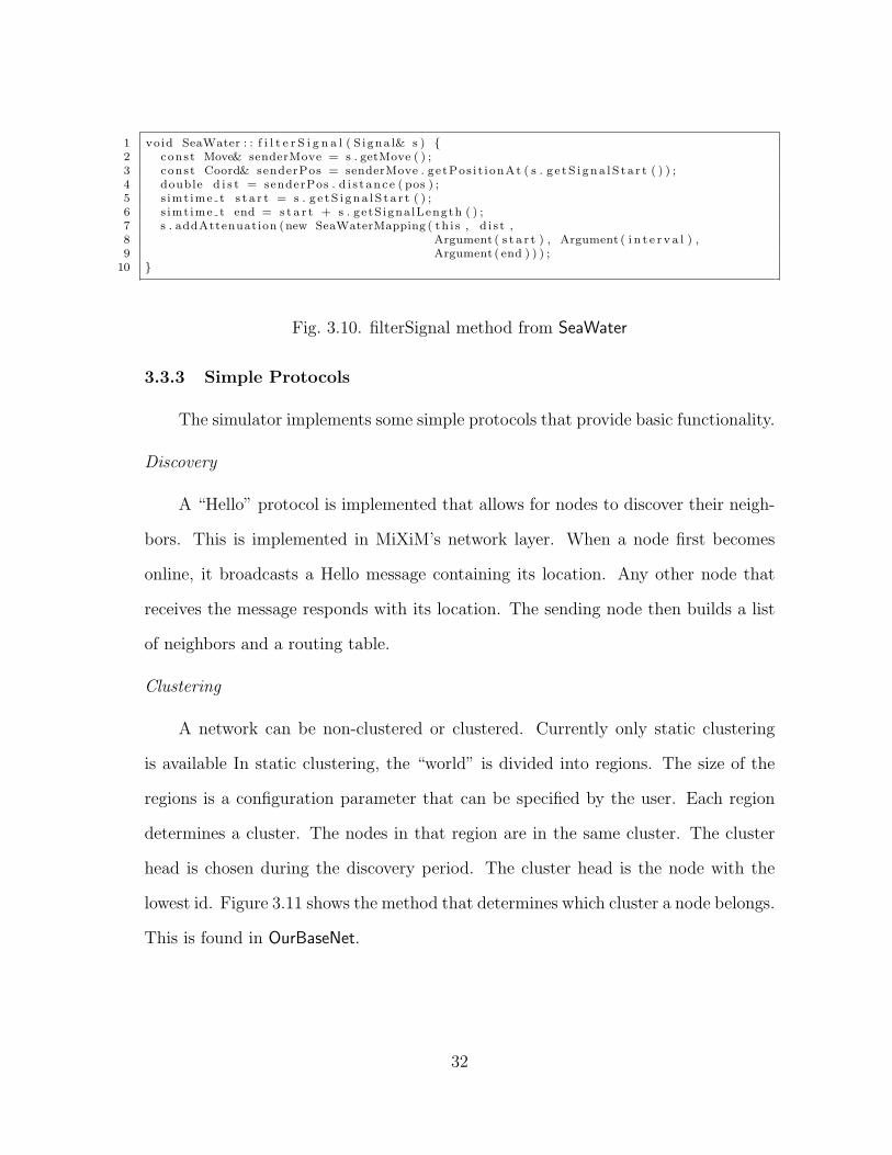
1 void SeaWater : : f i l t e r S i g n a l ( S i gna l& s ) {2 const Move& senderMove = s . getMove ( ) ;3 const Coord& senderPos = senderMove . ge tPos i t i onAt ( s . g e tS i gna l S t a r t ( ) ) ;4 double d i s t = senderPos . d i s t anc e ( pos ) ;5 s imt ime t s t a r t = s . g e t S i gna l S t a r t ( ) ;6 s imt ime t end = s t a r t + s . getS igna lLength ( ) ;7 s . addAttenuation (new SeaWaterMapping ( th i s , d i s t ,8 Argument ( s t a r t ) , Argument ( i n t e r v a l ) ,9 Argument ( end ) ) ) ;

10 }

Fig. 3.10. filterSignal method from SeaWater

3.3.3 Simple Protocols

The simulator implements some simple protocols that provide basic functionality.

Discovery

A “Hello” protocol is implemented that allows for nodes to discover their neigh-

bors. This is implemented in MiXiM’s network layer. When a node first becomes

online, it broadcasts a Hello message containing its location. Any other node that

receives the message responds with its location. The sending node then builds a list

of neighbors and a routing table.

Clustering

A network can be non-clustered or clustered. Currently only static clustering

is available In static clustering, the “world” is divided into regions. The size of the

regions is a configuration parameter that can be specified by the user. Each region

determines a cluster. The nodes in that region are in the same cluster. The cluster

head is chosen during the discovery period. The cluster head is the node with the

lowest id. Figure 3.11 shows the method that determines which cluster a node belongs.

This is found in OurBaseNet.

32

1 i n t OurBaseNet : : f i ndC lu s t e r ( ) {2 const Coord∗ pos = bb−>getPos ( ) ;3 const Coord∗ playground = world−>getPgs ( ) ;4 i n t g r i dS i z e = ( i n t ) world−>getGr idS i ze ( ) ;5 i n t x = ( i n t ) ( pos−>getX ( ) ) ;6 i n t y = ( i n t ) ( pos−>getY ( ) ) ;7 char bu f f [ 8 ] ;89

10 i n t xGrid = 0 ;11 i n t yGrid = 0 ;12 i n t pX = ( in t ) ( playground−>getX ( ) ) ;13 i n t pY = ( in t ) ( playground−>getY ( ) ) ;1415 f o r ( i n t i = 1 ; i <= pX/ g r i dS i z e ; i++) {16 i f ( x < i ∗ g r i dS i z e ) {17 xGrid = i ;18 break ;19 }20 }21 f o r ( i n t i = 1 ; i <= pY/ g r i dS i z e ; i++) {22 i f ( y < i ∗ g r i dS i z e ) {23 yGrid = i ;24 break ;25 }26 }2728 i n t s tep = ( i n t ) (255/(pX/ g r i dS i z e ∗ pY/ g r i dS i z e ) ) ;2930 i n t c l u s t e r = (pX/ g r i dS i z e )∗ ( yGrid−1) + xGrid ;31 s p r i n t f ( buf f , ”@%2.2X%2.2XAF” , s tep ∗( c l u s t e r ) , s tep ∗( c l u s t e r −1)) ;32 node−>ge tD i sp l aySt r ing ( ) . setTagArg (” i ” ,1 , bu f f ) ;33 node−>ge tD i sp l aySt r ing ( ) . setTagArg (” i ” , 2 , ”100” ) ;34 re turn c l u s t e r ;35 }

Fig. 3.11. findCluster method from OurBaseNet

Routing

The basic routing protocol that is provided uses distance between nodes to de-

termine the next hop. When a message is sent, the location of the receiver has to

be provided. The networking layer will determine the next hop for the message. If

the receiver is a neighbor, the message is sent directly to the receiver. If the receiver

isn’t a neighbor, the message is sent to the neighbor that is closest to the receiver.

A method was added to the connection manager that allows for a node to look up

the location of another node. It uses this information to determine how to route the

messages. Figure 3.12 shows the findRoute() method used to determine the host to

33

1 i n t OurBaseNet : : f indRoute ( i n t source ) {2 ev << ” f i nd route f o r ” << source << endl ;3 char bu f f [ 2 5 5 ] ;4 s p r i n t f ( buf f , ”node[%d ] ” , source ) ;5 cModule∗ other = s imu la t i on . getModule ( source)−>getParentModule ( ) ;6 const Coord∗ pos = cm−>getPos ( other−>get Id ( ) ) ;7 i f ( pos != NULL) {8 ev << ” po s i t i o n ” << pos−>i n f o ( ) << endl ;9 }

10 RTIterator i t ;11 bool f i r s t P a s s = true ;12 double d i s t ance = 0 . 0 ;13 i n t nextHop = −1;14 f o r ( i t = rout ingTable . begin ( ) ; i t != rout ingTable . end ( ) ; i t++) {15 double d = (∗ i t ) . second−>pos−>s q r d i s t ( pos ) ;16 i f ( f i r s t P a s s ) {17 f i r s t P a s s = f a l s e ;18 d i s t ance = d ;19 nextHop = (∗ i t ) . f i r s t ;20 } e l s e {21 i f (d < d i s t ance ) {22 d i s t ance = d ;23 nextHop = (∗ i t ) . f i r s t ;24 }25 }26 }27 re turn nextHop ;28 }

Fig. 3.12. findRoute method from OurBaseNet

forward the message to.

Applications

Two applications have been developed to demonstrate how the simulator works.

• The first applications has one node send a message to another node. The nodes

involved are read from the configuration file.

• The second application has nodes sending messages at random times to a sink.

The node that acts as the sink is specified in the configuration file.

3.4 UASim GUI

UASim is a Graphical User Interface (GUI) that builds configuration files for OM-

NeT++ and MiXiM without the user having to use the OMNeT++ IDE. The user

34

can select from predefined simulations and has access to most of the configuration

parameters that would be found in OMNeT++ “ini” file, normally called omnetpp.ini.

The GUI is implemented in Java. Java was chosen for portability reasons. All

internal configuration files are written in XML so JDOM is required for the GUI to

run. It also requires the Visual Swing package which was used in Eclipse for visual

development of the GUI.

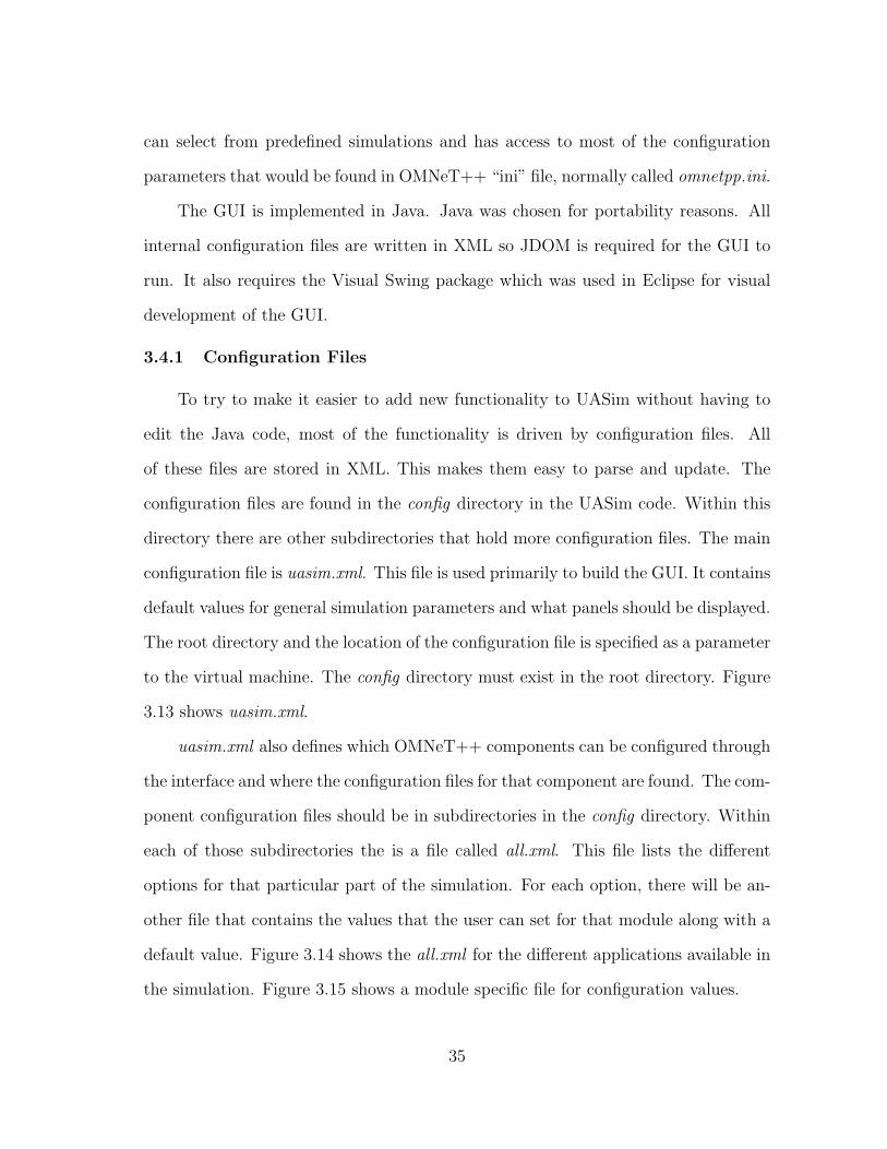
3.4.1 Configuration Files

To try to make it easier to add new functionality to UASim without having to

edit the Java code, most of the functionality is driven by configuration files. All

of these files are stored in XML. This makes them easy to parse and update. The

configuration files are found in the config directory in the UASim code. Within this

directory there are other subdirectories that hold more configuration files. The main

configuration file is uasim.xml. This file is used primarily to build the GUI. It contains

default values for general simulation parameters and what panels should be displayed.

The root directory and the location of the configuration file is specified as a parameter

to the virtual machine. The config directory must exist in the root directory. Figure

3.13 shows uasim.xml.

uasim.xml also defines which OMNeT++ components can be configured through

the interface and where the configuration files for that component are found. The com-

ponent configuration files should be in subdirectories in the config directory. Within

each of those subdirectories the is a file called all.xml. This file lists the different

options for that particular part of the simulation. For each option, there will be an-

other file that contains the values that the user can set for that module along with a

default value. Figure 3.14 shows the all.xml for the different applications available in

the simulation. Figure 3.15 shows a module specific file for configuration values.

35

1 <uasim>2 <!−− Tie in va lue s from the main sc r e en to the opt ion panel −−>3 <simTypes opt ionPanel=”Channel”>4 <simType name=”Underwater Acoust ic ” value=”ua” />5 <simType name=”T e r r e s t r i a l ” va lue=”r f ” />6 </simTypes>7 <de f au l t s >8 <numNodes>4</numNodes>9 <numRuns>1</numRuns>

10 <playgroundX uni t=”m”>500</playgroundX>11 <playgroundY uni t=”m”>500</playgroundY>12 <playgroundZ uni t=”m”>500</playgroundZ>13 <c l u s t e r S i z e un i t=”m”>125</ c l u s t e r S i z e >14 </de f au l t s >15 <!−− Def ine the pane l s that are a v a i l a b l e when con f i gu r i n g the16 s imu la t i on −−>17 <opt ionPanels>18 <panel name=”Appl i ca t ion ” t i t l e =”Conf igure the App l i ca t ion ” d i r=”app” />19 <panel name=”Networking” t i t l e =”Conf igure the Networking Layer” d i r=”net ” />20 <panel name=”MAC” t i t l e =”Conf igure the MAC Layer” d i r=”mac” />21 <panel name=”Phys i ca l ” t i t l e =”Conf igure the Phys i ca l Layer” d i r=”phy”22 s e l e c t e d=”simType” />23 <panel name=”Channel” t i t l e =”Conf igure the Channel” d i r=”chan”24 s e l e c t e d=”simType” />25 <panel name=”Mobi l i ty ” t i t l e =”Conf igure the Mobi l i ty Type” d i r=”mob” />26 </opt ionPanels>27 <!−− Def ine how to f i nd OMNet++ and MiXiM −−>28 </uasim>

Fig. 3.13. uasim.xml.

Per Node Configuration File

Node location is handled by the MiXiM’s mobility module and the default con-

figuration for a simulation run sets the nodes to random locations. Editing an om-

netpp.ini file in the OMNeT++ IDE allows for the user to configuration each node

individually. A way to do per node configuration was needed in UASim. The GUI

1 <a l l >2 <module name=”fromto” shor t=”Node to Node” f i l e =”fromto . xml” d e f au l t=”1”>3 Send message between two random nodes .4 </module>5 <module name=”to s ink ” f i l e =”to s ink . xml” shor t=”Node to Sink”>6 Nodes randomly send to s ink .7 </module>8 </a l l >

Fig. 3.14. An all.xml.

36

1 <appl p r e f i x=”node [ ∗ ] ” l a b e l=”Appl i ca t ion Layer Parameters ” type=”applType”2 value=”SendAppLayer” >3 <s ink >4</sink>4 <debug>f a l s e </debug>5 <burs tS i ze >3</burs tS i ze >6 <headerLength un i t=”b i t ”>512</headerLength>7 </appl>

Fig. 3.15. A configuration file for a UASim module.

1 0 mob i l i ty . x=300; mob i l i ty . y=300; mob i l i ty . z=02 1 mob i l i ty . x=600; mob i l i ty . y=600; mob i l i ty . z=03 2 mob i l i ty . x=600; mob i l i ty . y=10; mob i l i ty . z=04 3 mob i l i ty . x=10; mob i l i ty . y=600; mob i l i ty . z=05 playgroundX 7006 playgroundY 7007 playgroundZ 08 g r i dS i z e 7009 numNodes 4

Fig. 3.16. A per node configuration file.

allows the user to load a file containing per node configurations in addition to play-

ground and grid size values. A sample file is shown in Figure 3.16. Any node item can

be configured through the file including location, speed, network layer, MAC layer,

etc.

3.4.2 Classes

The class diagram for UASim is shown in Figure 3.17.

SimGUI

This is the main module for the GUI. It builds the base frame, the menu bar,

and the navigation buttons. It contains a tabbed pane that holds all of the

panels for simulation configuration.

Simulation

The Simulation class holds the configuration parameters for the simulation run.

It parses the main configuration file for UASim and stores the configuration

37

Fig. 3.17. Class diagram for UASim.

values. This class also builds the configuration files for OMNeT++ and runs

the simulation. Figure 3.18 shows the code to get the module parameters from

the panels and writes it to omnetpp.ini.

SimPanel

The SimPanel class builds the General configuration panel for UASim. It is

displayed as the first tab on the tabbed pane. It deals with parameters such as

number of nodes and how the simulation is run. Figure 3.19 shows the program

38

1 // now we need to i t e r a t e over the parameters from the c on f i gu r a t i on2 // tabs from the more opt ions s c r e en .3 i t = params . entrySet ( ) . i t e r a t o r ( ) ;4 whi l e ( i t . hasNext ( ) ) {5 Map. Entry pa i r s = (Map. Entry ) i t . next ( ) ;6 System . out . p r i n t l n ( pa i r s . getKey ( ) + ” ” + pa i r s . getValue ( ) ) ;7 // er i s the root o f the document and w i l l s p e c i f y the module8 // that has the parameters9 Element er = ( Element ) pa i r s . getValue ( ) ;

10 // l a b e l i s complete ly unnecessary , i t j u s t makes the f i l e look11 // pre t ty12 Att r ibute a = er . g e tAt t r ibute (” l a b e l ” ) ;13 i n i . p r i n t l n ( ) ;14 i f ( a != nu l l ) {15 i n i . p r i n t l n(”######### ” + a . getValue ( ) + ” ########”);16 } e l s e {17 i n i . p r i n t l n(”######### ” + pa i r s . getKey ( ) + ” parameters ########”);18 }19 // p r e f i x d e f i n e s i f the re i s an extra p i e c e o f in fo rmat ion that20 // needs to be part o f the parameter s t r i n g . Usual ly t h i s i s21 // something l i k e nodes [ ∗ ]22 a = er . g e tAt t r ibute (” p r e f i x ” ) ;23 St r ing p r e f i x = ”” ;24 i f ( a != nu l l ) {25 p r e f i x = a . getValue ( ) + ” . ” ;26 }27 // Type i s used f o r modules that can be s p e c i f i e d with l i k e in the28 // ned f i l e s . Value conta in s the name o f the module that should be29 // used .30 a = er . g e tAt t r ibute (” type ” ) ;31 i f ( a != nu l l ) {32 St r ing t = a . getValue ( ) ;33 a = er . g e tAt t r ibute (” value ” ) ;34 i f ( a != nu l l ) {35 i n i . p r i n t l n (” baseSim .” + p r e f i x + t + ” = \”” + a . getValue ( ) + ”\””) ;36 }37 }38 // The ch i l d r en conta in a l l o f the parameters f o r the s e l e c t e d module .39 // Pr int them to the i n i f i l e . L i s t par = ( L i s t ) e r . ge tChi ldren ( ) ;40 I t e r a t o r pI t = par . i t e r a t o r ( ) ;41 whi l e ( pI t . hasNext ( ) ) {42 Element e = ( Element ) pI t . next ( ) ;43 a = e . ge tAt t r ibute (” un i t ” ) ;44 St r ing value = e . getValue ( ) ;45 i f ( a != nu l l ) {46 value += a . getValue ( ) ;47 }48 a = e . ge tAt t r ibute (” func ” ) ;49 i f ( a != nu l l ) {50 value = a . getValue ( ) + ”(\”” + value + ”\” )” ;51 }52 i n i . p r i n t l n (” baseSim .” + p r e f i x + er . getName ( ) + ” .” +53 e . getName ( ) + ” = ” + value ) ;54 }55 }

Fig. 3.18. Code to get module parameters from the panel.

39

Fig. 3.19. General configuration tab of UASim.

with the SimPanel General tab displayed.

ConfigPanel

ConfigPanel holds the configuration information for an OMNeT++ component

like the physical layer or mobility module. A ConfigPanel consists of a list

of available modules and a table containing the configuration parameters for

the selected module. These panels are built dynamically using the information

found in the configuration files. The individual panels are specified in uasim.xml.

Panel information is read from the all.xml found in the directory specified in

uasim.xml. all.xml gives general information on the modules and the file that

contains the configuration parameters. This file is read to build the table.

Figure 3.20 shows one of the ConfigPanels displayed.

Module

40

Fig. 3.20. A configuration panel in UASim.

A Module contains a JDOM representation of the configuration options for an

OMNeT++ component.

ParamTableModel

ParamTableModel allows a Java JTable to hold a JDOM Element. The table

consists of two columns, a label and a value. Modifying a value in the table will

save the value back to the JDOM hierarchy.

SimConfigDisplay

This class displays a window with all of the current configuration settings for a

simulation run. It contains the buttons that will actually start the simulation

running. It is displayed when the “OK” button is clicked on the UASim window.

Figure 3.21 shows the SimConfigDisplay.

41

Fig. 3.21. The configuration display window.

Node

This class contains node specific configuration values. These values are written

out to the omnetpp.ini file prior to any of the other module information. This

ensures that the simulation determines the correct parameters for the node.

3.5 Evaluation and Results

This project was intended to provide a framework that would allow future researchers

to build their own simulations for underwater acoustic WSN. It should provide some

modules containing different protocols and applications to demonstrate functionality

of the simulator and an underwater acoustic channel. An interface should be provided

to configure and run simulations.

UASim has met most of its requirements. It is built on top of OMNeT++ and the

MiXiM framework which provides a GUI for development of new modules/algorithms,

42

visual and command line execution of simulations and visual representation of results.

UASim adds onto MiXiM by providing an underwater acoustic channel that allows

for the signal to attenuate correctly for sound underwater. A sample networking layer

is provided that includes discovery, clustering, and simple routing. MiXiM’s CSMA

module is used for the MAC layer. Sample applications are provided that drive the

simulations. All provided modules and many of MiXiM’s examples can also be used

as a basis for developing new algorithms.

The UASim GUI provides an easy way to configure a simulation while still pro-

viding the user the ability to change most parameters of a simulation. The GUI was

developed so new modules/algorithms could be added easily and with minimal or no

changes to the GUI code. The GUI can run the simulation once configured. The user

views simulation results in the OMNeT++ IDE.

3.5.1 Sample Simulation Runs

This section will discuss expected results and show actual simulation results for

the functionality of the simulator.

Connectivity

Because an Underwater Acoustic Simulation (UAS) is different from a Terrestrial

Simulation (TS), different connectivity is expected for a simulation with the nodes

located in identical positions. Because of the smaller frequency used underwater,

nodes further apart should be able to communicate. Figure 3.22 shows the General tab

and resulting node connectivity for terrestrial and underwater acoustic simulations.

Both simulations loaded the node file in Figure 3.16. No configuration parameters

were changed except for the network type.

43

(a) General tab for TS. (b) TS resulting connectivity.

(c) General tab for UAS. (d) UAS resulting connectivity.

Fig. 3.22. Differences in the connectivity for TS and UAS using the same simulation

configuration.

Static Clustering

In static clustering the playground is divided into square regions. Each node

calculates their cluster and sends that information to other nodes during the discovery

phase. The node also calculates its color based on the cluster. Nodes in the same

cluster will be the same color. The node with the lowest id is selected as the cluster

head. All nodes start marked with a star, but after the discovery phase, only the

cluster head will still have a star. Figure 3.23a shows the beginning of a simulation

44

with one cluster. The nodes are all the same color and marked with a star. Figure

3.23b shows the simulation after the discovery phase with only one cluster head.

Figure 3.24 shows a simulation run with four clusters and eight nodes.

(a) Nodes before discovery. (b) Nodes after discovery.

Fig. 3.23. Simulation with one cluster. After the discover phase, the node that displays

the star icon is the cluster head.

A Sample Simulation Run

Figures 3.25 through 3.30 show a simulation run. First the user runs the UASim

program which displays the General configuration tab shown in Figure 3.25a. The

user decides to load a per node configuration file shown in Figures 3.25b and 3.25c.

Figure 3.25d shows the new configuration parameters after loading the file. The

user then decides to change the frequency used in the connection manager. This is

illustrated in Figures 3.25e and Figure 3.25f. At this point the simulation is configured

and the user clicks on “OK”. The system displays a list of configuration parameters

(Figure 3.26). The user clicks on “Run”. UASim launches OMNeT++ in the visual

mode. Figure 3.27 shows that the underwater acoustic connection manager is being

used which also means that the underwater acoustic channel is used. Figure 3.28

shows the OMNeT++ window. The user starts the simulation by clicking on “Fast”

in the OMNeT++ window. Figure 3.29 shows the simulation running and Figure

45

Fig. 3.24. A simulation with four clusters and eight nodes. Nodes of the same color

are in the same cluster. Nodes with star icons are cluster heads.

3.30 shows that the simulation ended.

3.5.2 Known Issues

• Currently the underwater acoustic model used in simulations relies mainly on

attenuation of the signal. The model is basically MiXiM’s terrestrial model with

attenuation changes applied. The physical layer functions like the terrestrial

physical layer and still sends things call AirFrames. The NIC is a terrestrial

NIC. In the future it may be necessary to modify everything from the physical

layer down to model underwater hardware and conditions more realistically.

• Under Microsoft WindowsTM operating system, UASim is unable to launch

OMNeT++ when “Run” is pressed. This is an issue with Microsoft WindowsTM

operating system and Java and is yet to be resolved. The configured simulation

can be run by hand using the run.bat script generated by UASim. This script

is found in the config/run directory.

• Because of the generic way that the GUI is built, it isn’t validating all of the

46

(a) (b)

(c) (d)

(e) (f)

Fig. 3.25. Screen shots from UAsim. (a) initial UASim screen. (b) load a per node

configuration file. (c) file chooser when selecting a per node configuration

file. (d) General tab after per node configuration file is loaded. (e) select a

parameter to change. (f) modify a simulation parameter.

47

Fig. 3.26. The display of simulation parameters prior to running simulation.

Fig. 3.27. Output from OMNeT++ that shows the connect manager used.

Fig. 3.28. OMNeT++ simulation screen.

48

Fig. 3.29. A screen shot of the simulation running.

Fig. 3.30. End of simulation dialog.

simulation parameters. It will allow the user to set up a simulation that OM-

NeT++ may not be able to run or a simulation that runs, but doesn’t do

anything. Better validation and error checking is needed. This should be in the

GUI and the OMNeT++ modules.

• The nodes do static clustering and determine a cluster head. This information

is not used for any node functionality or routing.

49

4. CONCLUSIONS AND FUTURE WORK

Underwater WSN is an emerging field that requires much research in the areas of

sensor nodes, architecture, and protocols. To assist with this research, a simulator

that can handle underwater environments is needed. Many simulators for networking

applications exist, but at this time, there is only one that we know of that can

handle underwater acoustic sensor networks. This simulator does not easily run on

Microsoft WindowsTM operating system and is based on the ns-2 simulator which has

been superseded with ns-3.

This project implements an underwater WSN simulator that can also be used

for terrestrial WSN. This simulator is built on top of the OMNeT++ framework and

uses the MiXiM models for WSN. It contains an underwater acoustic channel and

provides sample applications and a networking layer to assist with future development

of modules. In addition to the simulation framework, a GUI was created that will

allow a user to easily configure a simulation run. The GUI utilizes configuration files

for easy addition of modules that may be developed for the simulator in the future.

Configuration parameters for individual nodes in the simulation can be loaded from a

file to give more control over node placement. The simulator runs on both Microsoft

WindowsTM operating system and Linux. It was tested on Microsoft WindowsTM 7

operating system and Gentoo Linux. It is expected to run on any OMNeT++ and

Java supported platform.

Results show that the GUI can correctly generate the configuration files needed to

run an OMNeT++/MiXiM simulation. It is also shown that a terrestrial and under-

water acoustic simulation with the same node configuration has different connectivity

between the nodes. This is expected because of the differences in the medium and

the frequencies of the signals.

The simulator is a good first step at providing a complete underwater acoustic

50

channel and a easy way to configure underwater acoustic simulations.

4.1 Future Work

The underwater acoustic channel currently relies on attenuation of the signal to rep-

resent an underwater simulation. Many parts of the physical layer and channel are

still too similar to a terrestrial counterpart. More work is needed to provide a better

underwater acoustic channel that more fully represents underwater conditions and

communications.

Not all of the initial requirements have been satisfied. The simulator lacks ability

to have multiple types of nodes. More node models should be developed as require-

ments for the nodes become available. In most cases creating a new NIC module

for the node maybe be sufficient. With the addition of multiple types of nodes, the

simulator would need to handle heterogeneous and homogeneous simulations. This

may require the development of additional connection managers. Dynamic clustering

has not been implemented.

Visualization of simulation results has not been fully explored. This system relies

on the abilities of OMNeT++ IDE to view results and the event log generated by a

simulation run. More work may be needed in this area. More logging may need to

be added to the modules to capture required metrics.

MiXiM 2.0 provides a new package called Mixnet that allows the user to use

both MiXiM and the INET framework together. INET provides many modules for

the upper network stack that MiXiM is missing. This could potentially allow for

many existing protocols to be used in our underwater acoustic environment. As this

ability in MiXiM matures, it should be investigated as it may increase the number

of protocols available for networking layer, application layer, etc, without having to

develop them locally.

51

DEDICATION

This work is dedicated to my husband, Scott King, and my son, Graham, who had

to put up with my general crabbiness while I pursued my Master’s degree. Without

their love and support this would not have been possible.

52

ACKNOWLEDGMENTS

I would like to thank the members of my committee, Dr Ajay Katangur, Dr

David Thomas and especially Dr Ahmed Mahdy (committee chair) for their time and

effort.

A special thanks goes to the developer’s of OMNeT++ and MiXiM, who saved

me from reinventing the wheel and provided a great foundation for my work.

53

BIBLIOGRAPHY AND REFERENCES

[1] A. Mahdy, “Marine wireless sensor networks: Challenges and applications,” In-ternational Conference on Networking, vol. 0, pp. 530–535, 2008.

[2] T. Schriber and D. Brunner, “Inside discrete-event simulation software: how itworks and why it matters,” in WSC ’99: Proceedings of the 31st conference onWinter simulation. New York, NY, USA: ACM, 1999, pp. 72–80.

[3] I. Akyildiz, D. Pompili, and T. Melodia, “Underwater acoustic sensor networks:research challenges,” Ad Hoc Networks, vol. 3, no. 3, pp. 257–279, May 2005.[Online]. Available: http://dx.doi.org/10.1016/j.adhoc.2005.01.004

[4] T. Voigt, F. Osterlind, N. Finne, N. Tsiftes, Z. He, J. Eriksson, A. Dunkels,U. Bamstedt, J. Schiller, and K. Hjort, “Sensor networking in aquatic environ-ments - experiences and new challenges,” in LCN ’07: Proceedings of the 32ndIEEE Conference on Local Computer Networks. Washington, DC, USA: IEEEComputer Society, 2007, pp. 793–798.

[5] I. Vasilescu, K. Kotay, D. Rus, L. Overs, P. Sikka, M. Dunbabin, P. Chen, andP. Corke, “Krill: An exploration in underwater sensor networks,” in EmbeddedNetworked Sensors, 2005. EmNetS-II. The Second IEEE Workshop on, May2005, pp. 151–152.

[6] I. Vasilescu, K. Kotay, D. Rus, M. Dunbabin, and P. Corke, “Data collection,storage, and retrieval with an underwater sensor network,” in SenSys ’05: Pro-ceedings of the 3rd international conference on Embedded networked sensor sys-tems. New York, NY, USA: ACM, 2005, pp. 154–165.

[7] M. Dunbabin, P. Corke, I. Vasilescu, and D. Rus, “Data muling over underwaterwireless sensor networks using an autonomous underwater vehicle,” in Roboticsand Automation, 2006. ICRA 2006. Proceedings 2006 IEEE International Con-ference on, May 2006, pp. 2091–2098.

[8] C. Detweiller, I. Vasilescu, and D. Rus, “An underwater sensor network withdual communications, sensing, and mobility,” in OCEANS 2007 - Europe, June2007, pp. 1–6.

[9] D. Anguita, D. Brizzolara, A. Ghio, and G. Parodi, “Smart plankton: a natureinspired underwater wireless sensor network,” in ICNC ’08: Proceedings of the2008 Fourth International Conference on Natural Computation. Washington,DC, USA: IEEE Computer Society, 2008, pp. 701–705.

[10] “Smart plankton,” November 2009. [Online]. Available:http://www.smartplankton.org/

[11] X. Che, I. Wells, P. Kear, G. Dickers, X. Gong, and M. Rhodes, “A staticmulti-hop underwater wireless sensor network using rf electromagnetic commu-nications,” Distributed Computing Systems Workshops, International Conferenceon, vol. 0, pp. 460–463, 2009.

[12] “The network simulator - ns2,” April 2011. [Online]. Available:http://www.isi.edu/nsnam/ns/

54

[13] S. Bajaj, L. Breslau, D. Estrin, K. Fall, S. Floyd, P. Haldar, M. Handley,A. Helmy, J. Heidemann, P. Huang, S. Kumar, S. McCanne, R. Rejaie,P. Sharma, K. Varadhan, Y. Xu, H. Yu, and D. Zappala, “Improving simulationfor network research,” University of Southern California, Tech. Rep. 99-702b,March 1999, revised September 1999, to appear in IEEE Computer. [Online].Available: http://www.isi.edu/ johnh/PAPERS/Bajaj99a.html

[14] “The ns-3 network simulator,” April 2011. [Online]. Available:http://www.nsnam.org/

[15] “Opnet modeler,” April 2011. [Online]. Available:http://www.opnet.com/solutions/network rd/modeler.html

[16] A. Varga and R. Hornig, “An overview of the omnet++ simulation environ-ment,” in Simutools ’08: Proceedings of the 1st international conference onSimulation tools and techniques for communications, networks and systems &workshops. ICST, Brussels, Belgium, Belgium: ICST (Institute for ComputerSciences, Social-Informatics and Telecommunications Engineering), 2008, pp. 1–10.

[17] C. Mallanda, A. Suri, V. Kuncharkarra, S. Iyengar, R. Kannan, and A. Durresi,“Simulating wireless sensor networks with omnet++,” 2005, submitted to IEEEComputer.

[18] A. Boulis, “Castalia user’s manual,” April 2011. [Online]. Available:http://castalia.npc.nicta.com.au/pdfs/Castalia%20-%20User%20Manual.pdf

[19] “Sense: Sensor network simulator and emulator,” April 2011. [Online].Available: http://www.ita.cs.rpi.edu/sense/index.html

[20] “Aqua-sim,” April 2011. [Online]. Available:http://ubinet.engr.uconn.edu/mediawiki/index.php/Aqua-Sim

[21] “Monarch project,” April 2011. [Online]. Available:http://www.monarch.cs.rice.edu/cmu-ns.html

[22] P. Xie, Z. Zhou, Z. Peng, H. Yan, T. Hu, J. Cui, Z. Shi, Y. Fei, and S. Zhou,“Aqua-sim: An ns-2 based simulator for underwater sensor networks,” inOCEANS 2009, MTS/IEEE Biloxi - Marine Technology for Our Future: Globaland Local Challenges, October 2009, pp. 1–7.

[23] “Omnet++,” April 2011. [Online]. Available: http://www.omnetpp.org/

[24] “Mixim,” April 2011. [Online]. Available: http://mixim.sourceforge.net/

[25] K. Wessel, M. Swigulski, A. Kopke, and D. Willkomm, “Mixim: the physicallayer an architecture overview,” in Simutools ’09: Proceedings of the 2nd In-ternational Conference on Simulation Tools and Techniques. ICST, Brussels,Belgium, Belgium: ICST (Institute for Computer Sciences, Social-Informaticsand Telecommunications Engineering), 2009, pp. 1–8.

[26] “Jdom,” April 2011. [Online]. Available: http://www.jdom.org/

55

APPENDIX A – USE CASE TEXTUAL DESCRIPTIONS

A.2 High-level Use Case

A.2.1 Configure Simulation

Title: Configure simulation

Actors: User

Preconditions: User has started simulator and is at main screen

Flow of Events:

• Main Successful Scenario

1. User enters general configuration values2. User enters module configuration values3. System maintains configuration values4. User presses OK button5. System displays configuration values

• Alternate Scenarios

1. Module missing(a) Steps 1-2 in main scenario(b) Desired module isn’t available(c) User selects different module

Postconditions: User is on configuration parameter display

A.2.2 Run Simulation

Title: Run simulation

Actors: User

Preconditions: User has the program running, has configured a simulation, and is onthe display configuration parameters screen

Flow of Events:

• Main Successful Scenario

1. User presses Run button2. System runs simulation3. System shows busy indicator while simulation is running4. System displays last selected tab when simulation finishes

• Alternate Scenarios

56

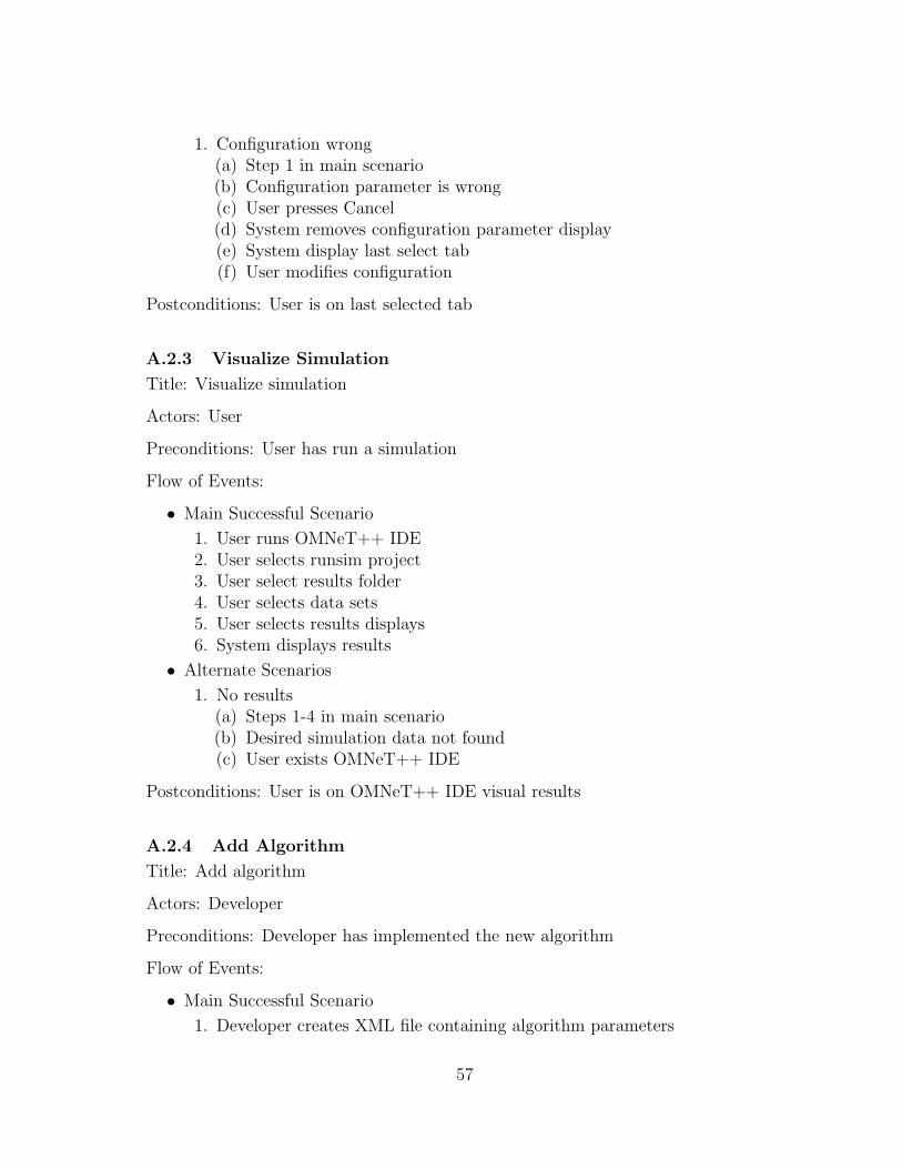
1. Configuration wrong(a) Step 1 in main scenario(b) Configuration parameter is wrong(c) User presses Cancel(d) System removes configuration parameter display(e) System display last select tab(f) User modifies configuration

Postconditions: User is on last selected tab

A.2.3 Visualize Simulation

Title: Visualize simulation

Actors: User

Preconditions: User has run a simulation

Flow of Events:

• Main Successful Scenario

1. User runs OMNeT++ IDE2. User selects runsim project3. User select results folder4. User selects data sets5. User selects results displays6. System displays results

• Alternate Scenarios

1. No results(a) Steps 1-4 in main scenario(b) Desired simulation data not found(c) User exists OMNeT++ IDE

Postconditions: User is on OMNeT++ IDE visual results

A.2.4 Add Algorithm

Title: Add algorithm

Actors: Developer

Preconditions: Developer has implemented the new algorithm

Flow of Events:

• Main Successful Scenario

1. Developer creates XML file containing algorithm parameters

57

2. Developer places XML file in appropriate directory3. Developer edits all.xml in appropriate directory4. Developer adds new algorithm to all.xml5. Developer saves all.xml6. System make available new algorithm when run

• Alternate Scenarios

1. System error saving all.xml(a) Steps 1-5 in main scenario(b) System can’t save file due to system error(c) Developer corrects system error

Postconditions: New algorithm is added to new system

A.3 Configure Simulation Use Case

A.3.1 Set Simulation Parameters

Title: Set simulation parameters

Actors: User

Preconditions: User has started simulator and is on General tab

Flow of Events:

• Main Successful Scenario

1. User selects network type2. User enters number of nodes3. User enter playground information4. User indicates if they want a visual run5. System maintains configuration changes

Postconditions: User is on General tab

A.3.2 Set Module Parameters

Title: Set module parameters

Actors: User

Preconditions: User has started simulator and is on General tab

Flow of Events:

• Main Successful Scenario

1. User selects tab to enter module specific configuration parameters2. System displays available modules with default selected

58

3. System display configuration parameters for selected module4. User selects desired module5. System displays configuration parameters for select module6. User changes desired configuration parameters7. System maintains changes

• Alternate Scenarios

1. Module missing(a) Steps 1-3 in main scenario(b) Desired module isn’t available(c) User selects a different module

Postconditions: User is on last selected tab

A.3.3 Load Node Data

Title: Load node data

Actors: User

Preconditions: User has created a per node configuration file and has started simulatorand is on General tab

Flow of Events:

• Main Successful Scenario

1. User presses File menu2. User selects Load Node Data option3. System displays a file chooser4. User selects configuration file and presses Open5. System closes file chooser6. System reads configuration file and keeps node data in memory7. System updates any general configuration parameters read from file8. User sees configuratino parameters updated

• Alternate Scenarios

1. File permissions wrong(a) Steps 1-6 in main scenario(b) System can open file because of permission problems(c) System displays error message(d) User acknowledges error message

Postconditions: User is on General tab with any changes displayed

59

A.3.4 Reset To Defaults

Title: reset to defaults

Actors: User

Preconditions: User has started simulator and has made changes to general configu-ration parameters

Flow of Events:

• Main Successful Scenario

1. User wants to reset changes2. User presses Reset To Defaults button3. System reset parameters to defaults read from configuration files4. System displays default parameters

Postconditions: User is on General tab with defaults displayed

A.4 Add Algorithm Use Case

A.4.1 Develop Module

Title: Develop module

Actors: Developer

Preconditions: Developer has OMNeT++, MiXiM, and UASim installed and workingcorrectly

Flow of Events:

• Main Successful Scenario

1. Developer implements new module in OMNeT++ IDE2. Developer debugs new module in OMNeT++ IDE3. Developer saves new module in OMNeT++ IDE

Postconditions: Developer has a new working module

A.4.2 Create Parameter Configuration File

Title: Create configuration files

Actors: Developer

Preconditions: Developer has a new working module

Flow of Events:

• Main Successful Scenario

60

1. Developer edits new XML configation file2. Developer adds configuration parameters with default values and units to

file3. Developer saves file4. Developer copies file to correct directory for module type

• Alternate Scenarios

1. Can’t save file(a) Steps 1-3 in main scenario(b) System can’t save file due to system error(c) Developer handles system error

Postconditions: Developer has created configuration file and placed it in the correctdirectory

A.4.3 Add Module To GUI Configuration

Title: Add module to GUI configuration

Actors: Developer

Preconditions: Developer has a new working module and has saved a parameterconfiguration file to correct directory

Flow of Events:

• Main Successful Scenario

1. Developer edits all.xml file in module type directory2. Developer adds item for new module3. Developer saves all.xml file4. Developer has added new module to simulation GUI

• Alternate Scenarios

1. Can’t save file(a) Steps 1-3 in main scenario(b) System can’t save file due to system error(c) Developer handles system error

Postconditions: Developer has added the new module to the simulation GUI

61

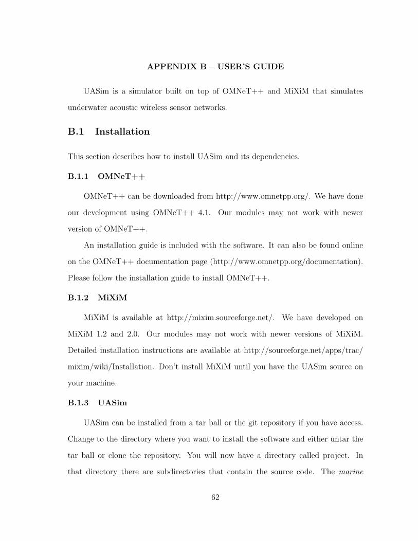
APPENDIX B – USER’S GUIDE

UASim is a simulator built on top of OMNeT++ and MiXiM that simulates

underwater acoustic wireless sensor networks.

B.1 Installation

This section describes how to install UASim and its dependencies.

B.1.1 OMNeT++

OMNeT++ can be downloaded from http://www.omnetpp.org/. We have done

our development using OMNeT++ 4.1. Our modules may not work with newer

version of OMNeT++.

An installation guide is included with the software. It can also be found online

on the OMNeT++ documentation page (http://www.omnetpp.org/documentation).

Please follow the installation guide to install OMNeT++.

B.1.2 MiXiM

MiXiM is available at http://mixim.sourceforge.net/. We have developed on

MiXiM 1.2 and 2.0. Our modules may not work with newer versions of MiXiM.

Detailed installation instructions are available at http://sourceforge.net/apps/trac/

mixim/wiki/Installation. Don’t install MiXiM until you have the UASim source on

your machine.

B.1.3 UASim

UASim can be installed from a tar ball or the git repository if you have access.

Change to the directory where you want to install the software and either untar the

tar ball or clone the repository. You will now have a directory called project. In

that directory there are subdirectories that contain the source code. The marine

62

directory contains the UASim pieces for OMNeT++. The uasim directory contains

the Java GUI. The runsim directory is a OMNeT++ project that the GUI uses to run

the simulations. The GUI will write configuration files in this directory and launch

simulations.

Next install MiXiM into the project directory. We do this by running the OM-

NeT++ IDE. Run omnetpp, when asked set the workspace to the the project direc-

tory that was installed for UASim (Figure B.1a) and press OK. When the OMNeT++

windows comes up, select the Workbench icon on the right hand side (Figure B.1b).

To import MiXiM. Select File→Import (Figure B.1c). In the Import window, open

the General folder and select “Existing Projects into Workspace” and press “Next”.

Choose “Select archive file” and browse to the location where MiXiM was down-

loaded. When the projects display, unselect Mixnet and press finish (Figure B.1d).

OMNeT++ will import MiXiM and start compiling. You will now have a MiXiM

directory in your project directory.

To add UASim to OMNeT++, select File→New→OMNeT++ Project (Figure

B.2a). Type in marine as the project name and press “Next” (Figure B.2b). Select an

“Empty project” as the template and press “Finish” (Figure B.2c). If you are asked

to overwrite any files, select “No”. marine will show up in the “Project Viewer”

on the left hand side of the OMNeT++ window. Right click on marine and select

“Properties” (Figure B.3a). Select “Project References” and check MiXiM (Figure

B.3b). Open the “OMNeT++” options and click on “Makemake”. Click on marine

in the middle box and then click on the “Options...” button (Figure B.3c). In the

Options window select “Shared library” and press “OK” (Figure B.3d). Follow the

same procedure to install the runsim directory. When adding “Project References”

select both MiXiM and marine. There is no need to set the Makemake options for

runsim.

63

(a) (b)

(c) (d)

Fig. B.1. OMNeT++ installation screen shots. (a) select a workspace. (b) OMNeT++

introduction screen. (c) import a project. (d) import an existion project.

64

(a)

(b) (c)

Fig. B.2. Installing UASim into OMNeT++. (a) add a new project menu options. (b)

name the new project. (c) select an empty template.

65

(a) (b)

(c) (d)

Fig. B.3. Installing UASim into OMNeT++. (a) add a new project menu options. (b)

name the new project. (c) select an empty template.

66

Now that all of the projects are loaded, select build all (Project→Build All) and

compile everything.

The GUI in uasim has a shell script and a bat file to launch the the program. It

comes with all of the necessary jar files to run.

B.2 Using UASim

UASim is a GUI developed in Java that will allows the user to configure a simulation

without using the OMNeT++ IDE. The GUI allows the user to access most of the

configuration parameters available in the IDE but it is easier to use.

The GUI is made up of different tabs that allow the user to configure a simulation

run. The user is able to load per node data also.

B.2.1 The General Tab

This tab allows for configuration of general simulation parameters. Figure B.4a

shows the General tab.

B.2.2 Other Configuration Tabs

The other tabs allow the user to configuration parameters for the specific modules

used in the simulation. These tabs will display the different options for each module.

When one of the options is selected the parameters for that option will be display in

the table. Any of the parameters can be changed to the desired value. Figure B.4b

shows one of the configuration tabs.

B.2.3 Loading Node Data

If the user wants to place nodes in specific locations, they enter the information

into a text file and then load it into the interface by selecting File→Load Node Data

and then they select the per node file in the file broswer. The format of the file is as

67

(a) (b)

Fig. B.4. UASim configuration tabs. (a) General tab. (b) Example of the other con-

figuration tabs.

follows:

node number parameter=value,parameter=value...

Configuration values for number of nodes, playground size, grid unit, and visual

run from the General tab can also be set in the file. Figure B.5 shows an example of

the per node file.

B.2.4 Running A Simulation

Once all of the simulation parameters have been selected the user can presses

the “OK” button. This will open a new window that displays the configuration

paramteres. If these parameters are set correctly, the user can run the simulation

1 0 mob i l i ty . x=300; mob i l i ty . y=300; mob i l i ty . z=02 1 mob i l i ty . x=600; mob i l i ty . y=600; mob i l i ty . z=03 2 mob i l i ty . x=600; mob i l i ty . y=10; mob i l i ty . z=04 3 mob i l i ty . x=10; mob i l i ty . y=600; mob i l i ty . z=05 playgroundX 7006 playgroundY 7007 playgroundZ 08 g r i dS i z e 7009 numNodes 4

Fig. B.5. A per node configuration file.

68

by pressing the “Run” button. This causes the GUI to write out the necessary

configuration files in the runsim directory and then it will launch either OMNeT++’s

Tkenv for a visual simulation or the Cmdenv for a command line simulation. If the

user is running a visual simulation, they will need start the simulation manually

(Figure B.6) and close out all of the OMNeT++ windows when the simulation is

done running.

Fig. B.6. Buttons to start visual simulation run.

B.2.5 Results

After running a simulation the event log and any captured metrics will be in run-

sim/results. The OMNeT++ IDE User Guide (http://omnetpp.org/doc/omnetpp41/

userguide/userguide.html) covers in detail how to use sequence diagrams on the event-

log and how to analyze results using the IDE.

69

APPENDIX C – PROGRAMMER’S GUIDE

The intent of our simulator was for researcher to be able to add new protocols

for testing. We provided some sample modules to use as a basis. In addition, many

of the MiXiM modules can be used. Adding new protocols is done in the OMNeT++

IDE and then configuration files in the UASim GUI are modified to include the new

protocols.

C.1 Required Tools

See the User’s Guide (Appendix B) for information on installing the base system.

You will need to install OMNeT++, MiXiM, and the UASim code. The OMNeT++

IDE can be used to edit, compile, run, and debug simulation modules. You will also

need a JRE or the Java SDK if you are plan to runthe UASim GUI.

C.1.1 Packages needed for GUI Development

The GUI requires Visual Swing and JDOM. The jar files for those are provided

with the UASim sources.

Eclipse and Visual Swing

The GUI was developed using Eclipse with the Visual Swing plugin. GUI devel-

opement in Java can be painful at best without a visual way to create any interfaces.

I selected Visual Swing and Eclipse because they were easy to use, some what familar

after using OMNeT++, and free.

JDOM

JDOM provides a “Java-based solution for accessing, manpulating, and out-

putting XML data from Java code” [26].

70

C.2 Adding to the Simulation Engine

It is best to have some familiarity with the tools that are being used. The Tictoc tu-

torial that comes with OMNeT++ is a good introduction to implementing modules in

OMNeT++. MiXiM provides a Beginner’s Guide and tutorials to help introduce how

their networks are implemented. These tutorials should give the developer enough

information to understand how to implement a new module in OMNeT++/MiXiM.

New modules for UASim should be added in the marine.

C.3 Modifications to the GUI

Unless changes are needed to the layout of the GUI or new configuration parameters

need to be added to the General tab, most additions to the GUI can be done through

the configuration files. All of the configuration files are in the uasim/config. The

main configuration file is uasim.xml. An example of the file is shown in Figure C.1.

This file lists what panels are should be added to the interface in the optionPanels

section. Each panel has a name and a title to display on the panel. It also specifies

the directory found in the config directory that contains the modules available on the

panel and configuration files for each module.

The simTypes section defines how the network selection on the General tab con-

trols values on the specified panel. This is used mainly to set the channel module to

the select network type on the General tab.

The defaults section defines default values for the fields on the General tab.

Each subdirectory contains module specific configurations. The all.xml file con-

tains the list of modules available. Each module has a name, a short description, the

file that contains the configuration values, if they are the default for the tab, and a

long description. The long description is displayed in a tooltip when the mouse hovers

71

1 <uasim>2 <!−− Tie in va lue s from the main sc r e en to the opt ion panel −−>3 <simTypes opt ionPanel=”Channel”>4 <simType name=”Underwater Acoust ic ” value=”ua” />5 <simType name=”T e r r e s t r i a l ” va lue=”r f ” />6 </simTypes>7 <de f au l t s >8 <numNodes>4</numNodes>9 <numRuns>1</numRuns>

10 <playgroundX uni t=”m”>500</playgroundX>11 <playgroundY uni t=”m”>500</playgroundY>12 <playgroundZ uni t=”m”>500</playgroundZ>13 <c l u s t e r S i z e un i t=”m”>125</ c l u s t e r S i z e >14 </de f au l t s >15 <!−− Def ine the pane l s that are a v a i l a b l e when con f i gu r i n g the16 s imu la t i on −−>17 <opt ionPanels>18 <panel name=”Appl i ca t ion ” t i t l e =”Conf igure the App l i ca t ion ” d i r=”app” />19 <panel name=”Networking” t i t l e =”Conf igure the Networking Layer” d i r=”net ” />20 <panel name=”MAC” t i t l e =”Conf igure the MAC Layer” d i r=”mac” />21 <panel name=”Phys i ca l ” t i t l e =”Conf igure the Phys i ca l Layer” d i r=”phy”22 s e l e c t e d=”simType” />23 <panel name=”Channel” t i t l e =”Conf igure the Channel” d i r=”chan”24 s e l e c t e d=”simType” />25 <panel name=”Mobi l i ty ” t i t l e =”Conf igure the Mobi l i ty Type” d i r=”mob” />26 </opt ionPanels>27 <!−− Def ine how to f i nd OMNet++ and MiXiM −−>28 </uasim>

Fig. C.1. uasim.xml.

over the module name. When a module is select the configuration file is opened and

the values are loaded into the table. Figure C.2 shows a sample all.xml.

The module specific files contain a prefix that should be written to the configu-

ration file with the value, a label that is written as a comment to the configuration

file, the type of the module and the module name. Each configuration parameter is

written with units and if it needs to be written as a function (this is for the configu-

1 <a l l >2 <module name=”fromto” shor t=”Node to Node” f i l e =”fromto . xml” d e f au l t=”1”>3 Send message between two random nodes .4 </module>5 <module name=”to s ink ” f i l e =”to s ink . xml” shor t=”Node to Sink”>6 Nodes randomly send to s ink .7 </module>8 </a l l >

Fig. C.2. An all.xml.

72

1 <appl p r e f i x=”node [ ∗ ] ” l a b e l=”Appl i ca t ion Layer Parameters ” type=”applType”2 value=”SendAppLayer” >3 <s ink >4</sink>4 <debug>f a l s e </debug>5 <burs tS i ze >3</burs tS i ze >6 <headerLength un i t=”b i t ”>512</headerLength>7 </appl>

Fig. C.3. A configuration file for a UASim module.

ration files for the Analogue models). Figure C.3 shows module specific configuration

file.

New modules should be added to all.xml in the appropriate subdirectory and a

configuration file containing the parameters should be added to the directory. After

that is done the GUI will display the new module as an option when it is run next.

73