A simplified credit risk model for supervisory purposes in ... · A simplified credit risk model for supervisory purposes in emerging markets, ... distribution, so that the ... default

Restricted

A simplified credit risk model for supervisory purposes in emerging markets, that measures concentration risk and explicitly relates credit risk to capital adequacy and single obligor limits 1

A simplified credit risk model for supervisory purposes in emerging markets, that measures concentration risk and explicitly relates

credit risk to capital adequacy and single obligor limits1.

Javier Márquez Diez-Canedo.

Abstract

Current credit risk methodologies rely extensively on numerical methods to obtain the portfolio loss distribution, so that the determination of risk measures such as VaR, capital requirements and single obligor limits, is an empirical process that requires a considerable amount of information and computational effort. This makes them difficult to apply and implement by financial authorities for regulatory purposes in emerging markets where information is scarce and of poor quality, and where computational resources may be limited. The measurement of risk concentration in loan portfolios and the identification of segments that exhibit excessive concentration, is a problem that has remained elusive despite its recognized importance.

Assuming default probabilities of the loans and their correlations are given exogenous parameters, a default model is developed which obtains a closed functional form for the loss distribution, under the premise that it can be characterized by its mean and its variance. The resulting explicit mean-variance representation of Value at Risk (VaR) provides a lower bound on the banks’ capitalization ratio and the resulting inequality establishes capital adequacy. The “Herfindahl-Hirshman” index emerges as a measure of numerical loan concentration, providing a precise quantification of how concentration contributes to overall credit risk of the portfolio. Two new properties of the index are obtained that relate single obligor limits to concentration along different segments of the portfolio so as to ensure capital adequacy. Furthermore, the effect of default correlation on concentration is analyzed and a measure of risk concentration is proposed.

Throughout the paper, the implications for risk management and regulation are discussed. Numerical exercises performed to date on real portfolios provide results comparable to those obtained using other methodologies, at a considerable reduction in computational effort. This is specially attractive for application to emerging markets where the type of information required by the more standard credit risk measurement methodologies is not available. In the final section, the results obtained from the model are illustrated through the analysis of credit risk in the Mexican Banking system.

Keywords: Capital adequacy, loan concentration risk, Herfindahl-Hirshman concentration index, single obligor limit, value at risk, default models.

1. Introduction2

Currently, the mainstream methodologies that are most widely used to measure credit risk can be classified into two broad categories; namely: Mark to Market models and Default models. The differences between these paradigms rest first on the scope of the losses considered. Whereas in default models an obligor can be in only one of two states, default and non-default, so that losses are exclusively those resulting from debtor defaults, mark to market models also consider losses resulting

1 An earlier versión of this model was Published in English in Economia, Societa’ e Istituzioni. See Márquez 2002. The model

presented here is an updated version with significant differences with the original and several new results. 2 A good detailed review of the different approaches is presented by M. Crouhy et al., JBF (24) 2000.

Restricted


from a change of value of the loans due to credit quality migration. Further differences arise from the functional forms assumed for the underlying probability distributions, and the way in which these are related to obtain the loan portfolios’ loss distribution. For example3, in CreditMetricsTM which is a mark to market methodology, the key component is the transition matrix related to a rating system, which provides the probabilistic mechanism that models the quality migration of loans. This determines the losses due to obligor defaults, and the changes in the market value of the loans in the portfolio due to quality migration through a Montecarlo simulation process, to finally obtain the loss distribution for the portfolio. Whereas the transition matrix, the changes of value and the loss given default of the loans, and the migration covariance’s are theoretically estimated from statistical data and market information, the simulation process relies heavily on a normality assumption around the transition probabilities and Merton’s4 asset value model to establish a relation between credit quality and asset value of the debtor firms, and to determine the joint migration behavior of the loans in the portfolio.

KMV’s5 methodology is also based on Merton’s model6 by defining a “distance to default”, which is the difference between the value of a companies assets and a certain liability threshold, such that if this quantity is negative, the company is bankrupt and will therefore default on its obligations. For standardization purposes, this distance to default is measured as a multiple of the standard deviation of the value of the firms’ assets. KMV has accumulated a large database, which it uses to estimate default probabilities and correlation’s, as well as the loss distributions due to debtor default and quality migration. For a specific company, this probability is approximated by the “expected default frequencies”; i.e. the ratio of the number of companies with the same distance to default that actually defaulted, to the total number of companies with the same distance to default in the database. Being a mark to market methodology, it differs significantly from CreditMetricsTM in that it relies on “EDF’s” for each debtor rather than average transition rates as estimated from the historical data produced by the rating agencies. There are also considerable differences in the assumptions and the functional forms utilized.

CreditRisk+ is a default model7 in which the cornerstone of the methodology is the set of individual default probabilities of the loans in the portfolio. A basic assumption is that the default probabilities are always small, so that the number of defaults in the portfolio can be approximated according to a Poisson probability distribution. In its more general version, where default probabilities can change over time, it is further assumed that these probabilities are entirely driven by a weighted sum of “K risk factors” each distributed according to an independent Gamma distribution. The weights of the risk factors differ depending on the individual rating of the obligor and, conditional on these risk factors, individual obligor defaults are assumed to be independent Bernoulli trials. In the general case, default correlation is implicit in the covariation behavior of the risk factors, and the Poisson assumption leads to a Negative Binomial for the distribution of the number of defaults. Having obtained the distribution of the number of defaults in the portfolio, proceeding in the typical actuarial fashion, by selecting a unit of loss and given the recovery rates for the individual loans, these are then grouped into buckets of equal loss given default, and the probability generating function of the loss distribution is obtained. From here it is necessary to resort to a numerical recursion procedure to obtain the loss distribution.

Another popular default methodology is Credit Portfolio View8, which is a discrete multi-period model. Apart from the fact that it is conceived from the beginning as a dynamic model, the highlight of the methodology is the determination of default probabilities, which are logit functions of indices of macro-economic variables. The portfolio is segmented according to geographical location and economic activity of the debtors, and the indices for each segment are linear functions of the associated macro-economic variables for the segment. In turn, each macro-economic variable is assumed to obey a 2nd order univariate, autoregressive process, and due to cross correlation’s in the

3 CreditMetrics TM is a spin-off from the J.P. Morgan Risk Management systems development group. 4 The reader unfamiliar with the methodology is referred to section 8 of the CreditMetrics TM technical document and Robert

Merton, 1974. 5 This is the proprietary methodology of KMV corporation. 6 See Kealhoffer 1998 and 1999. 7 CreditRisk+ is marketed by Credit Suisse Financial Products. 8 This product is offered by McKinsey, the consulting firm. The classical reference is Wilson (I) & (II) 1997.

Restricted


error terms of the linear models for the indices and the autoregressive expressions of the underlying macro-economic variables, the parameters of both are estimated simultaneously from a system of equations. Credit Portfolio View also resorts to simulation on transition matrices to obtain the loss distribution.

All of the above methodologies have contributed greatly to the understanding of the key issues in credit risk modeling and it is now accepted that all models are converging to produce comparable results. Research by Crouhy et. al. (2000), Finger (1998) and Gordy (2000) discuss how under certain parametric equivalents the mainstream methodologies such as CreditMetricsTM and CreditRisk+ can be mapped into each other. It is important to note that the emphasis in all of these methodologies is in producing a distribution of losses, which is as realistic as possible. Although one can hardly argue against this principle, the computational effort required can be impractical for certain users, such as regulators, who have to oversee the whole financial system, and not just one individual bank. Furthermore, the development of management tools such as obtaining simple rules for establishing capital adequacy, identifying segments of excessive credit risk concentration and setting single obligor limits to loans, that are explicitly related to the risk profile of the portfolio, is not directly addressed.

The model presented here assumes that the default probabilities of the loans and their covariance’s are given. From here, a default model is developed which obtains an explicit functional form for the loss distribution, assuming that it can be characterized by two parameters: The mean and the variance. Given a specific mean-variance distribution of losses, not necessarily Normal, it is possible to obtain the Value at Risk (VaR) for the portfolio as the expected loss plus a certain multiple of the standard deviation of losses. This leads to a lower bound on the banks’ capitalization ratio and the resulting inequality establishes capital adequacy. The model is developed in a way, which explicitly measures the concentration of the loan portfolio. It is seen that the “Herfindahl-Hirshman” index emerges naturally as a measure of concentration, providing a precise quantification of how concentration contributes to the overall credit risk of the portfolio. Two new properties of the index are obtained that relate single obligor limits to concentration along different segments of the portfolio so as to ensure capital adequacy. Furthermore, the research shows how correlation affects concentration and this leads to the definition of a risk concentration measure. Finally, it is shown that the model can be implemented with limited information on the actual composition of bank loan portfolio’s, which is a crucial factor for regulators insomuch as their capacity to obtain up to date and timely information from banks is limited.

Examples of numerical exercises performed to date on real loan portfolios are shown, and are seen to provide results comparable to those obtained using other methodologies, at a considerable reduction in computational effort. Finally, since all the relevant elements for measuring default credit risk are explicitly parameterized, the shortcomings of available information can be compensated by a judicious use of assumptions on the values of the relevant parameters. The computational efficiency of the model results in rapid feedback on the implications and sensitivity of the risk profile of a loan portfolio to changes in the parameters.9 Since the measurement of concentration is at the heart of the model, we begin with a discussion of this topic.

2. The concentration issue.

Loan concentration has long been identified as an important source of risk for banks and loan portfolios. Judging from current technical literature on credit risk, as far as concentration goes, the establishment of a generally accepted paradigm has remained elusive in spite of the importance of the problem10. The more formal approaches which look to portfolio theory11, have been mainly concerned with optimal diversification of portfolios of traded fixed income assets where information compatible with traditional Markowitz (1959) type models can be obtained in a cost effective manner. It must be pointed out however, that traditional portfolio theory approaches deal with the concentration issue

9 Due to the closed form expression for value at risk, it is also possible to perform analytical exercises. 10 See Caouette, Altman, y Narayanan 1998, chapters 17 and 18. See also Kealhofer 1998 . 11 See for example Bennet 1984.

Restricted


indirectly, since the preoccupation is the allocation of assets through the well known mean-variance tradeoff, but a clear measure of concentration and its relation to risk has never been made explicit. Kealhoffer (1998) has an interesting discussion of the issue from the point of view of diversification. First he states that “there has been no method for actually measuring the amount of diversification in a debt portfolio”, and that “ex-ante, no method has existed which could quantify concentrations”; concentrations have only been detected ex-post. He then argues that “measuring diversification means specifying the range and likelihood of possible losses associated with a portfolio”. He goes on to provide a definition that allows the comparison of diversification of two portfolios as:

“Portfolio A is better diversified than portfolio B if the probability of loss exceeding a given percentage is smaller for A than for B, and both portfolios have the same expected loss”.

Thus, when dealing with portfolios of traditional bank loans, no formal methodology for measuring concentration seems to have emerged. As pointed out by Altman and Saunders (1998), the concentration measurement issue has mainly been dealt with through subjective analysis. Typically, banks and other agents apply a scoring technique based on the opinion of a group of experts, about the degree of concentration observed along and across different segments of a portfolio, as regards to some classification criterion, in order to obtain an indicator of loan concentration. Generally, the number obtained is of more value in cardinal or hierarchical terms, than it is as a direct measure of risk that can quickly be translated into potential losses or value at risk12.

The approach adopted in the following analysis does not solve all the aforementioned problems, but it does provide a theoretical framework that might allow ex-ante, the detection of risk concentration. The proposed risk concentration measure is consistent with Kealhoffers’ notion as previously stated. Example 6.2 illustrates how the risk concentration measure can be used to detect the more risky segments of a loan portfolio.

3. Value at risk, Concentration and the “single obligor” limit: The simplest case.

Traditionally, banks deal with concentration risk by placing a limit on the maximum amount that can be loaned to a single debtor, along the different dimensions where concentration can occur; that is: By industry, geographical region, product, country etc. Normally, the “single obligor limit” is expressed as a proportion “δ” of the capital “K” of the bank. However, when discussing loan concentration, one normally addresses the issue of how much of the total loans outstanding is concentrated in an individual or group. Thus, whatever the virtues of setting limits as a percentage of capital, this does not give much information as to the actual concentration of loans in the portfolio. To see this, note that at least theoretically, a bank could have only one loan that respects the limit but have a totally concentrated portfolio. On the other hand, the bank can have a million uncorrelated loans of exactly the same size, in which case the portfolio would be completely diversified, regardless of whether each loan respects the limit or not. Thus, one can have highly concentrated portfolios as well as highly diversified portfolios that respect the constraint in terms of capital.13 We will therefore part with tradition, since for the purpose at hand it is better to think of concentration in terms of proportions of the total value of the loan portfolio, and fix limits accordingly. Throughout this paper, individual limits on loans will be expressed as proportions “θ” of the total value of the loan portfolio “V”. Furthermore, no generality is lost since δ andθ are linearly related, so the results are not altered. To see this, let “fk” denote the value of the kth of “N” loans, and analyze the single obligor limit as represented by the following constraint:

12 See for example Moody’s Investor services 1991, and the 1993 Coopers and Lybrand report. 13 For example, if loans are constrained not to exceed 12% of capital, this can be done with only one loan in the portfolio in

which case concentration is maximum. On the other hand, if the portfolio has a thousand loans all representing 12% of capital, it would be a highly diversified portfolio.

Restricted


VVVVK

Kf k θψδδδ ==•=≤ ; k = 0,1,2,3,....,N ....(3.1)

where VK

=ψ is the capitalization ratio. Thus,θ = δψ14, and the single obligor limit will be expressed

as:

fk ≤ θV ……k = 1,2,….,N

If all loans have the same default probability “p”, and assuming independence, one can define “N” binary random loss variables “xi” as:

fi with probability p xi = 0 with probability 1-p

Clearly E(xi) = pfi and Variance(xi) = p(1-p)fi2. Since the variables are independent:

a) pVpfxEN

ii

N

ii ==

= ∑∑

== 11

µ ; where V =∑=

N

iif

1

b) ∑∑∑===

−==

=

N

ii

N

ii

N

ii fppxVariancexVariance

1

2

11

2 )1()(σ

Since the distribution of loans (fi) is totally arbitrary, it is difficult to know the exact distribution of ∑=

N

iix

1

.

For the moment, assume that it can be approximated by the Normal distribution 15, so that:

∑=

−+=+=N

iifppzpVzVAR

1

2)1(ααα σµ ......(3.2)

If VARα ≤ K, after a bit of algebra one arrives at the following expression:

( )( )

( )αψψ

α

,,1

)(2

2

2

1

1

2

pppz

p

f

fFH

N

ii

N

ii

Θ=−

−≤

=

∑

∑

=

= ....... (3.3)

In this expression, portfolio concentration measured is measured by:

( ) 2

1

1

2

==

∑

∑

=

=

N

ii

N

ii

f

fFHionConcentrat

14 Note that if there is only one loan in the portfolio, then it is necessarily true that fi = V so that ψδ = ? = 1 which in turn implies

that the portfolio is totally concentrated in one loan. 15 See for example DeGroot (1988), p. 263.

Restricted


Readers familiar with the literature of industrial organization will have recognized that the above measure is the “Herfindahl-Hirshman” concentration index.16

4. Analysis of the Capital Adequacy Inequality.

The first observation is that, with the obvious limitations, it seems that portfolio concentration risk can be managed using a very general measure of concentration, other than the single obligor limit. Next, it is interesting to note that capital adequacy as represented by the capitalization ratio ψ requires that

( )FHppzp )1( −+≥ αψ .....(4.1)

This inequality relates capital adequacy to the probability of default, the confidence level used for value at risk, and the concentration index. It also shows that there is a direct relation between Herfindahls’ index and the variance of losses. Since the index takes on values between the reciprocal of the number of loans N, and one, where high concentration is present, the variance of losses will

vary between Npp /)1( − and )1( pp − , depending on H(F). Furthermore, note that the role

played by H(F) in the above is totally consistent with Kealhoffers’ definition of concentration since it is obvious from (4.1) that the lower the value of H(F), the lower the probability of loss exceeding a specified level, for the same expected loss.

In what follows, it is seen that everything behaves as it should. The following theorem summarizes the main implications for risk managers of the previous analysis. These results are introduced early because they remain basically unchanged throughout all future generalizations.

Theorem 4.1.

The bound Θ(p,ψ,α) on the concentration measure has the following properties:

Θ(p,ψ,α) varies in direct proportion to the capitalization ratioψ and inversely to the default probability “p” and the value at risk confidence level “zα”.

If the concentration measure exceeds the bound (i.e. H(F) > Θ(p,ψ,α)), then the capital of the bank is at risk, for the given confidence level.

If the default probability “p” exceeds the capitalization ratio “ψ”, then the capital of the bank is at risk for any confidence level, regardless of the concentration of the loan portfolio.

If Θ(p,ψ,α) > 1, no degree of concentration of the loan portfolio, places the capital of the bank at risk.

Proof.

Point one is obvious from the form of Θ(p,ψ,α). The second point is easily verified; that is: If H(F) > Θ(p,ψ,α) then,

( ) ( ) ( )KV

pqzppqz

pVpqzpVpqFzpVAR =

−+=Θ+>+=

α

αααα

ψθ )(

16 See for example Shy (1995) or Tirol (1995)

Restricted


Point three follows directly from 4.1:

VARα ≤ K ⇔ ( ) )(1 FHppzp −+≥ αψ

Point three is also verified easily. If p > ψ, then 4.1 is violated:

( )( ) ( )( ) KpqHVzKVpqFHzVpqHzpVAR >+=+>+= )(FF αααα ψ

As for point four, it is well known that H(F) ≤ 1 for any arbitrary F17.g

Capital adequacy Theorem 4.1 provides some useful rules for the risk manager and for the regulator. First, can be determined because one obtains precise measures of the adjustments in the capitalization ratio required by variations in the default rates and/or the concentration of the loan portfolio. Furthermore, depending on the amount of control that banks have on the default ratio and loan concentration, adjustments in the default probability and the concentration of the loan portfolio necessary to maintain capital adequacy can also be calculated. Thus, if the concentration of the loan portfolio exceeds the bound at the desired confidence level, inequality (3.2) provides a convenient means of fine tuning the adjustments required in ψ, p and H(F) so that credit risk does not place the capital of the bank in jeopardy. Also interesting, is that if the default rate of the portfolio exceeds the capitalization ratio, a signal of alarm is sent to the risk manager and the financial authorities, that the banks’ capital is at risk regardless of the concentration of the loan portfolio and the confidence level adopted.

5. A closer look at Herfindahls’ index.

One of the main features of the approach taken is that a measure of loan concentration as it relates to risk arises naturally. The Herfindahl-Hirschman index has been extensively studied in relation to industrial concentration, and it is known to have several important properties. Thus, it is known that the index takes values between the reciprocal of “N” and one18, and that it behaves well in terms of “the five properties of inequality measures”. 19 We now investigate how Herfindahls’ index relates to the intuitive notion that concentration is related to the minimum number of obligors where credit is more concentrated. A better understanding of the relation between the single obligor limit and the concentration index has important risk management and regulatory implications.

In order to examine how concentration relates to the notion that more credit in less hands means more concentration, it must be consistent with the notion that maximum concentration occurs when all credit is held by a single obligor and the minimum is when all debtors owe the same amount. Formally:

a) The maximum concentration occurs when for some “i”, one has that:

V for j = i fj = 0 for j≠ i; j = 1,2,....,N

i.e. Fmax = Vei , where ei ∈ EN is the ith unit vector.

b) The minimum concentration occurs when NV

f i = for i = 1,2,....,N

17

See Encaoua and Jacquemin 1980. 18 A simple normalization is possible, where it is easily seen that φ(F) as defined below, satisfies 0 ≤ φ ≤ 1

( ) ( )1

1

−

−=

NFH

NFφ

19 See Cowell 1995 and Encaoua and Jacquemin 1980.

Restricted


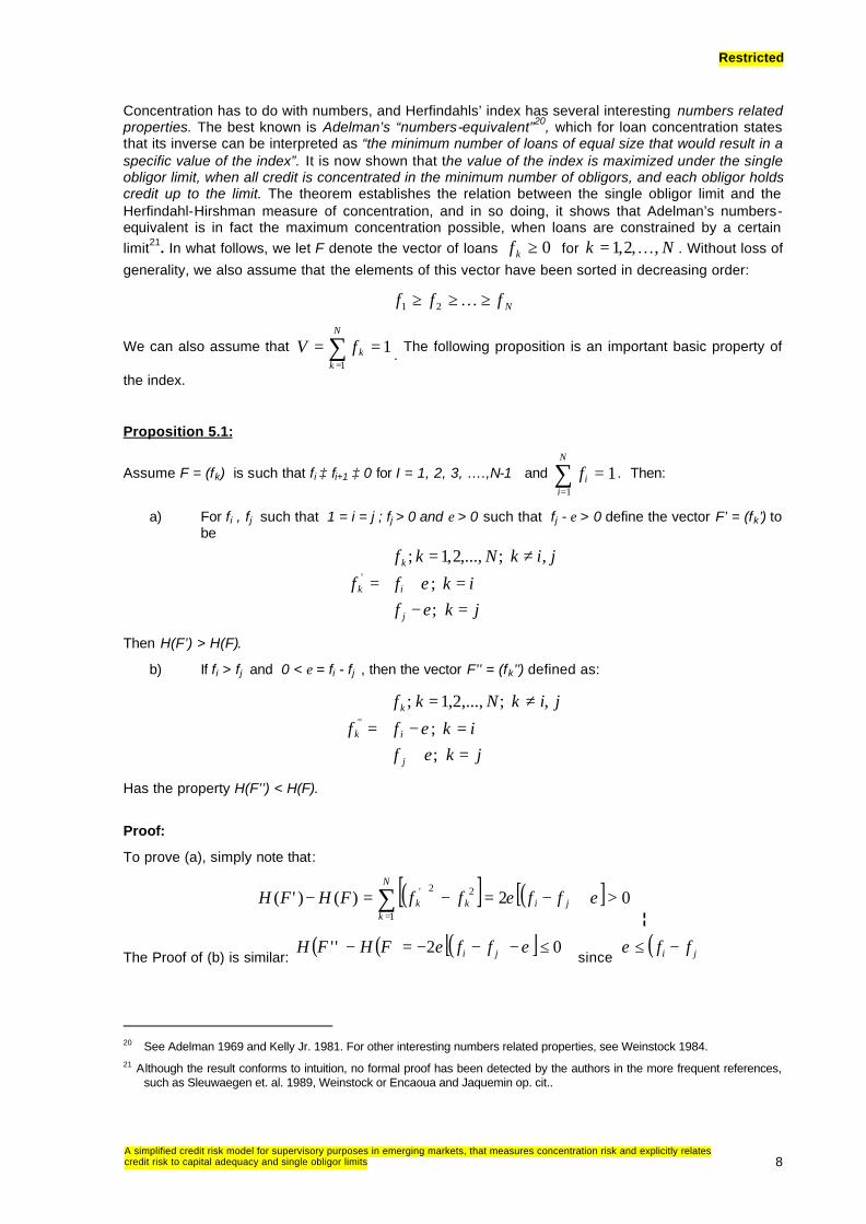
Concentration has to do with numbers, and Herfindahls’ index has several interesting numbers related properties. The best known is Adelman’s “numbers-equivalent”20, which for loan concentration states that its inverse can be interpreted as “the minimum number of loans of equal size that would result in a specific value of the index”. It is now shown that the value of the index is maximized under the single obligor limit, when all credit is concentrated in the minimum number of obligors, and each obligor holds credit up to the limit. The theorem establishes the relation between the single obligor limit and the Herfindahl-Hirshman measure of concentration, and in so doing, it shows that Adelman’s numbers-equivalent is in fact the maximum concentration possible, when loans are constrained by a certain limit21. In what follows, we let F denote the vector of loans 0≥kf

for Nk ,,2,1 K= . Without loss of

generality, we also assume that the elements of this vector have been sorted in decreasing order:

Nfff ≥≥≥ K21

We can also assume that ∑=

==N

kkfV

1

1 . The following proposition is an important basic property of

the index.

Proposition 5.1:

Assume F = (fk) is such that fi ≥ fi+1 ≥ 0 for I = 1, 2, 3, ….,N-1 and 11

=∑=

N

iif . Then:

a) For fi , fj such that 1 = i = j ; fj > 0 and ε > 0 such that fj - ε > 0 define the vector F’ = (fk’) to be

=−=+

≠=

=jkf

ikf

jikNkf

f

j

i

k

k

; ;

, ;,...,2,1 ;'

εε

Then H(F’) > H(F).

b) If fi > fj and 0 < ε = fi - fj

, then the vector F’’ = (fk’’) defined as:

=+=−

≠=

=jkf

ikf

jikNkf

f

j

i

k

k

; ;

, ;,...,2,1 ;''

εε

Has the property H(F’’) < H(F).

Proof:

To prove (a), simply note that:

( )[ ] ( )[ ] 02)()'(1

22' >+−=−=− ∑=

εε ji

N

kkk ffffFHFH

¦

The Proof of (b) is similar: ( ) ( ) ( )[ ] 02'' ≤−−−=− εε ji ffFHFH

since ( )ji ff −≤ε

20 See Adelman 1969 and Kelly Jr. 1981. For other interesting numbers related properties, see Weinstock 1984. 21 Although the result conforms to intuition, no formal proof has been detected by the authors in the more frequent references,

such as Sleuwaegen et. al. 1989, Weinstock or Encaoua and Jaquemin op. cit..

Restricted


(Note that ε > fi – fj implies case (a)). ¦

The proposition states that if some element fk is increased at the expense of decreasing a smaller element fj, the concentration index will increase. If on the other hand, an element is increased at the expense of a larger element, then the concentration index will decrease. To continue with the analysis, it is now shown that if all credit is concentrated in the minimum number of debtors, while subject to the constraint fk ≤ θ V, then H(F) ≤ θ.

Proposition 5.2:

Let ?∈ (0,1) and

=θ1

n be the integer part of θ1

. Let ε ∈ [0, 1) be such that n

εθ

−=

1. Then,

for the distribution,

+=

=

=else

nk

nk

f k

01;

,,2,1;

ε

θ L

we have that H(F) = ?.

Proof:

Note that ∑ fk = n? + ε = 1 and therefore:

( ) ( ) ( ) 1211 22222 +−+=++=+= θθθθεθ nnnnnnFH

For H(F) = ? one must solve the quadratic equation,

( ) θθθ =+−+ 121 2 nnn i.e. ( ) ( ) 01211 2 =++−+ θθ nnn ….. (5.1)

It is simple to verify that (5.1) has the following two solutions:

n1

1 =θ y 1

12 +

=n

θ

This means that if ?-1 is an integer, then H(F) = ?. Thus, examine what happens in the interval

+ nn1

,1

1

. To do this, let

( ) ( )( )11

11

1+

+=

+−+

=

nnn

nnλ

λλλθ with ( )1,0∈λ .

Substituting ?(?) in the left hand side of (5.1), one obtains:

( ) ( ) ( ) ( )

( ) ( ) ( ){ } ( )( ) ( )1,0 0

11

21212n 1

1

11

211

1

222

2

∈∀<+−

=+++−+−+++

=++

++−

+

++

λλλ

λλλ

λλ

nnnnnnnn

nn

nnn

nnn

nnn

¦

It is now shown that if all loans respect the single obligor limit fk ≤ θ V, then H(F) ≤ θ and the distribution of loans of the previous proposition maximizes the value of the index under the single obligor constraint.

Restricted


Theorem 5.3:

Let F = (fk) be such that:

+=+=

=

=Nnk

nk

nk

f k

,...,2 ;01 ;

,...,2,1 ;

ε

θ

with ?, ε ≥ 0; ε < ? and 1=∑ kf

. Then F maximizes H(F) for all F such that fk =?∀ k and H(F) =?.

Proof22:

Proposition 5.2 states that H(F) = ? for this distribution. Necessarily

=θ1

n and 0≥ε is such that

nε

θ−

=1

in order to have 1=∑ kf

. Furthermore, any vector with 0 ;' >+= δδθkf

would

violate the constraint kf k ∀≤ θ

. Therefore, the only possibility of altering the distribution of loans would be to decrease some element fk = ? or fn+1 = ε by some quantity δ > 0. But then proposition

5.1(b) states that H(F’) < H(F) = ?. ¦

This result has important implications for risk management and regulation since de facto, it states that by placing a limit on individual loans as a propotion of the value of the portfolio, one is also placing a limit on concentration as measured by Herfindahls’ index by the same amount θ. Therefore, it is simple to check for capital adequacy by

( )( )

( )αψψ

θα

,,12

2

pppz

pΘ=

−−

≤ ……(5.2)

Alternatively, from (4.1), one can obtain the capital adequacy relation in terms of the single obligor limit (2.6); that is:

θψ α )1( ppzp −+≥

.......(5.3) Thus, (5.2) provides a very simple means to check for capital adequacy, without doing complicated calculations. Although crude, simply take θ to be the ratio of the largest loan to the total value of the loan portfolio and the observed default rate as an ex-post proxy of default probability and substitute these values in the right hand side of (5.1). Since Theorem (5.1) guarantees H(F) ≤ θ, if the inequality holds it is a good sign that the bank is adequately capitalized.

It should be realized however, that this condition is sufficient but not necessary. As will be shown in the following theorem, if one chooses to explicitly constrain the portfolio to satisfy H(F) ≤ θ, it is possible to have specific loans that as a proportion of the total value of the portfolio represent a quantity larger than θ. Intuitively, granting a very large loan while satisfying the constraint on the index is only possible at the expense of the other loans in the portfolio so that in the optimum, the portfolio is composed only of one large loan and all others are small and of equal size.

22 This proof and the one for the next theorem are different from the original proofs in Márquez 2002. They are due to Fausto

Membrillo and are more intuitive and elegant than the original.

Restricted


Theorem 5.4:

If H(F) ≤ θ then:

( )( )( ) θθ <−−+≤ 1111

NNN

f i for i = 1,2,3,....,N

Proof:

The idea behind the proof is that under the constraint H(F) ≤ θ, a very large loan is only possible at the expense of all the other loans which must become progressively smaller and of equal size. So, given the constraint H(F) ≤ θ, let us maximize the largest element f1. Suppose f1 = a is the largest loan possible, then necessarily f2 = f3 = …. = fN = b; for some b > 0; b < a. To see this, consider any other distribution with fi > fj and 1 < i < j. Then there exists ε > 0 such that fi’ = fi - ε > fj’ = fj + ε > 0 . proposition 5.1 then states that H(F’) < H(F) = ?. Now, by continuity of the index on each fi and

because of theorem 5.3, there exists ε’ > 0 such that any loan distribution F’’ with '1''

1 ε+= ff and

0'''' ≥−= εjj ff satisfies θ≤< )''()'( FHFH , which contradicts the assumption that F is a

distribution where f1 is a maximum. Therefore, if f1 = a, for some a > 0, the loan distribution which maximizes f1, subject to the constraint H(F) ≤ θ, can be represented as

a ; k = 1 fk =

b ; k = 2, 3, ....,N

and a > b; therefore :

θ≤−+= 22 )1()( bNaFH …….(5.4)

Furthermore a + (N-1)b = V. solving for b:

11

−−

=N

ab

Substituting b en (5.4) one obtains:

( ) θ≤

−−

−+2

2

11

1Na

Na

This leads to the following quadratic equation:

( )[ ] 01122 ≤−−+− NaNa θ …..(5.5) Equating to zero, the solution of (5.5), yields:

( )( )[ ]1111

−−+= NNN

a θ

Note that a → √? when N → ∞, and it is simple to obtain the last inequality:

( ) 01 2 >−θ ⇔ 0122 >+− θθ ⇔ θθθ 4122 >++ ⇔ ( ) θθ 41 2 >+ ⇔ θθ 21 >+ ⇔

NN θθ 2)1( −<+− ⇔ 121)1( 22 +−<++− NNNN θθθθ ⇔

( )22 11 −<+−− NNNN θθθ ⇔ ( )21)1)(1( −<−− NNN θθ ⇔

1)1)(1( −<−− NNN θθ ⇔

( ) θθ <−−+ )1)(1(11

NNN g

Restricted


Having a good concentration index is desirable from the regulatory point of view, since it facilitates comparisons of loan concentration between different institutions, and it leads to an assessment of concentration risk for the financial system as a whole. For the risk manager of an individual bank, besides measuring his own risk, it provides benchmarks for setting business strategy and goals, and allows comparisons with the competition. Herfindahl’s index seems particularly well suited for the task, since besides measuring concentration it is directly related to risk, and provides a quick means to check capital adequacy. In the following section it will be seen that the concept is robust under much more general conditions.

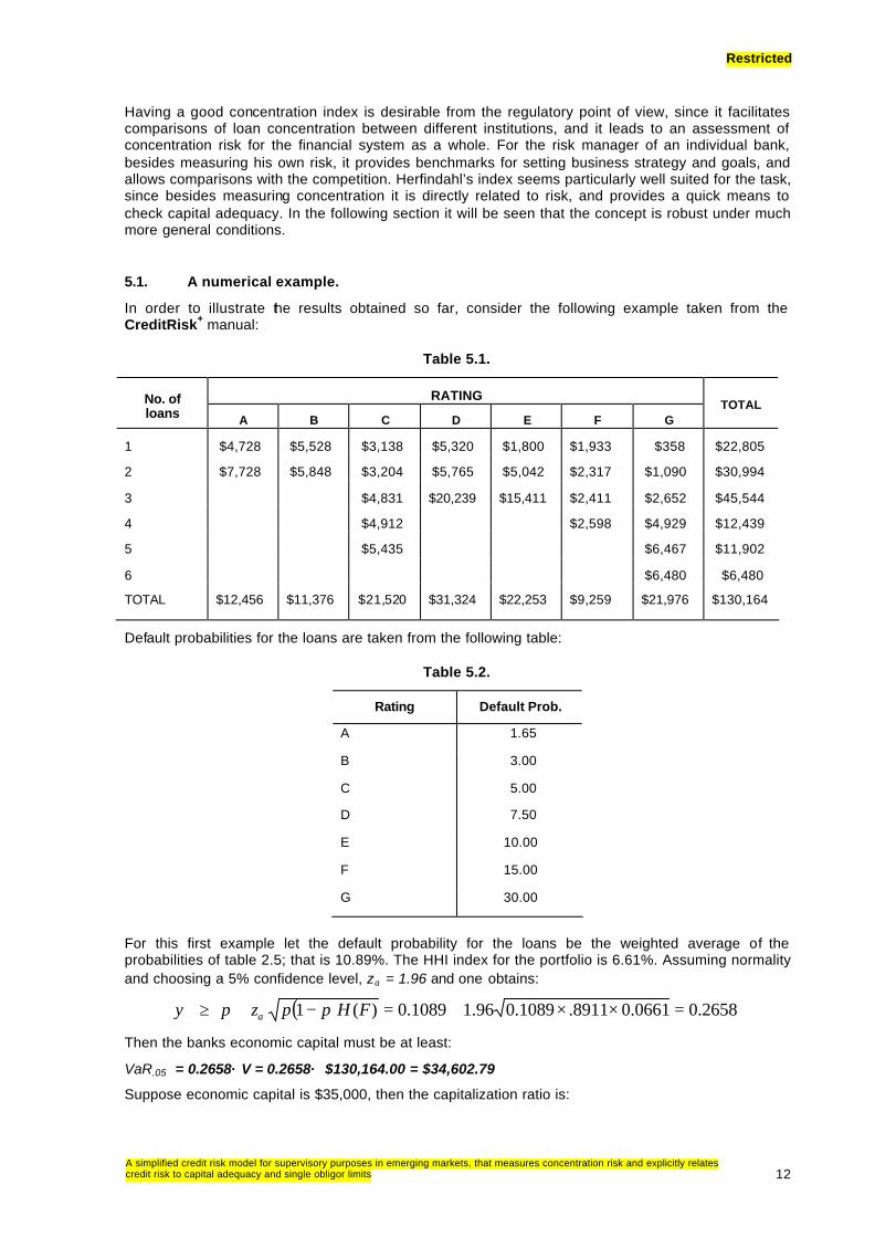
5.1. A numerical example.

In order to illustrate the results obtained so far, consider the following example taken from the CreditRisk+ manual:

Table 5.1.

RATING No. of loans A B C D E F G

TOTAL

1 $4,728 $5,528 $3,138 $5,320 $1,800 $1,933 $358 $22,805

2 $7,728 $5,848 $3,204 $5,765 $5,042 $2,317 $1,090 $30,994

3 $4,831 $20,239 $15,411 $2,411 $2,652 $45,544

4 $4,912 $2,598 $4,929 $12,439

5 $5,435 $6,467 $11,902

6 $6,480 $6,480

TOTAL $12,456 $11,376 $21,520 $31,324 $22,253 $9,259 $21,976 $130,164

Default probabilities for the loans are taken from the following table:

Table 5.2.

Rating Default Prob.

A 1.65

B 3.00

C 5.00

D 7.50

E 10.00

F 15.00

G 30.00

For this first example let the default probability for the loans be the weighted average of the probabilities of table 2.5; that is 10.89%. The HHI index for the portfolio is 6.61%. Assuming normality and choosing a 5% confidence level, zα = 1.96 and one obtains:

( ) 2658.00661.08911.1089.096.11089.0)(1 =××+=−+≥ FHppzp αψ

Then the banks economic capital must be at least:

VaR.05 = 0.2658× V = 0.2658× $130,164.00 = $34,602.79

Suppose economic capital is $35,000, then the capitalization ratio is:

Restricted


2689.0164,130000,35

===VK

ψ

Since 0.2689 > 0.2658, the bank exhibits capital adequacy. Now, under 3.2, the maximum concentration that the port folio can assume is:

( )( )

( )0687.0

8911.01089.096.11089.02689.0

1 2

2

2

2

=××

−=

−−

ppzp

α

ψ

Since H(F) = 6.61%, the portfolio is not excessively concentrated.

Since the maximum value of the index is 6.87%, no loan in the portfolio should exceed:

88.107,34164,1302621.00687.0* =×=×= Vf

Table 5.1, shows that the largest loan is the $20,239 D-loan, which is smaller than the aforementioned quantity. It is interesting to note that the single obligor limit would be violated. According to 5.2, loans should not exceed:

fi ≤ 0.0687× 130,164 = $8,942.27

There are two loans in the portfolio that are greater than this amount; namely the $20,239 D-loan and the $15,411 E-loan, confirming that the condition is sufficient but not necessary. Finally, it is seen that the largest loan in the portfolio is within the bounds provided by Theorem 5.2; that is: $8,942.27 ≤ $20,239 ≤ $34,107.88. §

6. Accounting for default correlation and different default probabilities.

The results obtained so far rely on the following assumptions:

a) The loss distribution can be characterized by its mean and variance.

b) Default probabilities are homogenous and independent from each other, for all loans along the dimension where loan concentration can occur.

c) There is only one dimension of possible loan concentration.

d) Nothing is recovered from defaulting loans.

In this section the model is generalized by relaxing the second and third assumptions. We first examine the case where default probabilities can be different and are correlated.

6.1 A General Model.

Assume that the portfolio loss distribution can be characterized by its mean and its variance and that the vector of default probabilities “π” and the Co-variance matrix “M” are given exogenously. Proceeding along the same lines of the previous analysis, the VaR to capital inequality is now:

KzVAR T ≤+= FMFF Tαα π ....(6.1)

Since M is positive definite, it is well known that there exists a Matrix “Q” such that,

TQQM Λ= ......(6.2)

Restricted


where Λ is the diagonal matrix of characteristic values of M, and Q is an orthogonal matrix of the

eigen-vectors of M, with the property that Q-1 = QT.23 Let TQQS Λ= , where Λ is the diagonal

matrix of the square roots of the eigen-values of M, so that SSM T= . Now change the variable to G = SF so that FTMF = GTG. This change of variable effectively rescales “F” in terms of the matrix “S” which in turn is representative of the “square root” of the covariance matrix “M”. It is well known that this is equivalent to rescaling the loans in the portfolio according to the covariances of the default probabilities between the loans, so that loans with higher loss covariances will increase in size, while the opposite will happen to loans with smaller loss covariances. Although much credit in few hands is potentially dangerous, it is even more dangerous when too much risk is concentrated in a particular group of debtors, as suggested by the rescaling of the loan portfolio in terms of “S ”. Thus, in a given moment a numerically highly diversified portfolio of small loans that exhibit large variances and are highly correlated, may be riskier than a numerically small portfolio of large loans that are uncorrelated and have low default probabilities. In the next section, the discussion is taken a step further.

To continue with the development of the model, multiplying and dividing FTMF by FTF, and dividing by

F1T=V , the following capital adequacy relation, relative to the value of the loan portfolio is obtained:

( ) ( )FHzpFHFF

MFFzp T

T

σψ αα +=+≥ .....(6.3)

where

),(2 MFRFTF

MFTF==σ = Rayleigh’s Quotient .....(6.4)

is a measure of the standard deviation of losses and

Vp

T Fπ= .......(6.5)

is the expected loss of the portfolio relative to its value which is nothing more then the weighted average of default probabilities. Proceeding in the usual way, and applying theorem 5.1, one obtains a limit on concentration and single obligor limits as:

( )2

−≤≤

σψ

θαz

pFH .......(6.6)

Note that relations (6.3) and (6.6) have the same structure as those obtained for the simple cases of equal default probabilities and independent loans. In this general case, Rayleigh’s quotient measures the variance of losses. One can verify that this reduces to the case of equal default probabilities for all loans and uncorrelated defaults, and that all the results of Theorem 4.1 are still true under this generalization.

Note that the total variance of losses ( )FHσ , is decomposed into the variation-covariation effect,

represented by σ, and concentration H(F). This emphasizes the fact that resizing the loan vector through the co-variance matrix “M”, implies that concentration in the number of loans is not necessarily a good measure of risk concentration.

23 Any intermediate text on matrix theory can be consulted. See for example Strang G. 1980, or Mirsky L. 1990.

Restricted


6.2. A measure of risk concentration.

In order to investigate how correlation affects concentration and increases risk, consider the special case when all loans have the same default probability “p” and each pair of loans is similarly correlated through “ρ”. Then, the covariance of defaults between any two loans (i,j) is:

jipppppp ijjjiiijjiij ,)1()1()1( ∀−=−−== ρρρσσσ .......(6.7)

In this case the covariance matrix has the following structure:

−⋅=

1

11

)1(

ρρρ

ρρρ

LOOM

MOL

ppM ......(6.8)

It is convenient to represent this as:

( ){ }I11M T ρρ −+−= 11 p)p( .......(6.9)

Thus, the variance of losses of the portfolio is:

( ) ( ){ }FFF1MFF TTT ρρ −+−= 112

p)p(

Proceeding in the usual way, and noting that V = 1TF, this leads to a VaR of:

{ })()1()1( FHppzpVVaR ρρα −+−⋅+= ......(6.10)

In this expression, loss variance is decomposed into two distinct elements. The first is the Bernoulli variance p(1-p), while concentration is captured by:

)()1(' FHH ρρ −+= .... (6.11)

Note that under positive correlation, H’ can be interpreted as a convex combination between the HHI of a totally concentrated portfolio (H(.) = 1) and the HHI of the portfolio H(F). Clearly, H’ increases with “ρ” and for ρ = 0 we have H’ = H(F); whereas H’ =1 if ρ = 1. In other words, if all the loans of a portfolio are perfectly and positively correlated, in terms of risk they behave as a single loan. In general, one can say that the correlated portfolio behaves exactly the same as an uncorrelated portfolio, whose concentration index is H’, instead of H(F). Thus, H’ could be considered a correlation adjusted concentration index.

Furthermore, (6.11) can be used to compute such an index for any given portfolio by computing “p” and“ρ”, such that:

( ) [ ] )(),()()1()1('1 FHFMRFHppHpp ⋅=−+⋅−⋅=⋅− ρρ ......(6.12)

Letting V

pT Fπ

= , solving for ρ gives:

[ ][ ])(1)1(

)()1(),(

1)(

1

1)1(),(

FHppFHppFMR

FH

ppFMR

−−⋅−⋅−

=

−

−

−⋅=ρ ......(6.13)

The expression provides an equivalent correlation measure which summarizes how loan defaults are pairwise correlated within the portfolio.

Restricted


Example 6.1

Consider the loan portfolio of the previous examples. The correlation matrix used in this exercise is as shown in appendix A, and is segmented into three groups:

=

32313

32212

31211

MCCCMCCCM

M

,,

,,

,,

Assuming normality and a 5% confidence level, VaR is:

$55,683 6)1.96(21,1714,17905.05. =+=+= MFTT FzFVaR π

From previous examples we know that p = 0.1089, H(F) = 0.0661, and computation yields:

0.6329 0.4006 ===FF

MFFT

T

σ

Thus, capital adequacy requires:

0.4278)F(Hzp =σ+>ψ α

Assume K = $60,000, so that 4610.0164,130000,60

==ψ . Relation (1.5), provides single obligor limits:

0805.09)1.96(0.632

0.1089-0.4610z

p22

=

=

σ

−ψ≤θ

α That is:

482,10$164,130$0805.0f i =×≤ From table (7.2) it is seen that there are only two loans that exceed the limit.

Let us now examine the impact of correlation on concentration. From (6.13):

[ ][ ] 2191.0

0661.010978.00661.00978.04006.0

=−×

×−=ρ

From (6.11), the risk concentration index is:

H’ = 0.2191 + (1-0.2191)×0.0661 = 0.2707

Beside the fact that the portfolio of this example is a pretty bad one, if one adds 22% correlation to the

high default probability of 10.89% one obtains unexpected losses of 1627.0)F(H =σ , as opposed

to 0801.0)()1( =− FHpp if the loans were independent. Thus, the 22% equivalent correlation

doubles the standard deviation of losses over the uncorrelated case. It is also interesting to compare the risk concentration index of H’ = 27.07%, which is four times greater than H(F) = 6.61%. In terms of capital adequacy, the correlated portfolio requires a capitalization ratio ψ ≥ 43% which is substantially greater than the 27% required if the loans were independent.§

6.3. Dealing with Different Dimensions of Concentration.

Generally, banks partition loan portfolios into sub-portfolios or “buckets” according to some practical criterion which is somehow related to the way in which they do business. For the purpose of credit risk in general and concentration in particular, it may be desirable to adopt different criterion. As mentioned initially, one of the most difficult problems is to determine ex-ante, potentially dangerous dimensions of concentration, and these may have nothing to do with the organizational structure of the bank. The model permits a totally arbitrary segmentation of the portfolio, in order to determine the segments

Restricted


where concentration is potentially riskier. This permits the differentiation of limits for each segment, as well as differentiation in the allocation of capital.

6.3.1. The analysis of individual segments.

Suppose that F is arbitrarily partitioned into “h” segments, ( )hT FFF ,...,1= , where Fi is a vector

whose elements are the amounts outstanding of the loans in group “i”. Now partition the default probability vector and the associated covariance matrix accordingly:

a) ( )iππ = ; where “πi” is the vector of default probabilities of segment i; i

= 1,2,3,....,h

b) The covariance matrix is partitioned as:

=

hhh

nh

h

MCC

CMCCCM

LMOMM

LL

21

2221

1121

M

Each diagonal block Mi is the covariance matrix of defaults for the loans in segment “i” and has dimension (Ni×Ni); where Ni is the number of loans in the segment. Matrices “Cij” contain the

covariances of the defaults between the loans of segments “i” and “j”. Let ∑∈

=iFj

ji fV , be the value of

the portfolio of segment “i”, and VVh

ii =∑

=1

. Let Ki = γiK, where “γi” is the proportion of capital

allocated to segment “i”; [ ] ∑=

=∀∈h

iii i

1

1;1,0 γγ . Note that when analyzing individual segments,

only correlations between defaults of the loans in segment “i” with loans of the other groups should be considered, while correlations of other groups between themselves are irrelevant. Thus, from “M” construct matrices “Si” with the following structure:

Si =

00

2

00

21

1

1

LLMLMLM

LLMLMLM

LL

hi

ihii

i

C

CMC

C

…. (6.14)

Note that MSi i =∑ . When integrating the analysis of individual segments into the overall portfolio,

it is important that the relative weights of each segment in the overall portfolio do not distort the results for the portfolio as a whole. An additivity property is necessary so that addition of over individual segments is consistent for the portfolio. Let

∑=

= h

i 1

FSF

MFF

iT

T

φ …. (6.15)

In what follows, we will se that this constant permits the summation of the individual VaRi. Proceeding in the usual way, the value at risk inequality for each segment is:

KKz iiiT

iii γφν α =≤+= FSFFpT for i = 1,2,…,h (6.16)

Restricted


Where γi ≥ 0 y 1=∑ i iγ . It is easily verified that FMFF Tαα πν zVaR T

i i +==∑ .

Dividing by Vi, leads to capital adequacy for each individual segment:

( ) ( )( ) { }

∑≠

++=≥ijj

jTiiii

i

ii HRzp

V /2

1, FCF

F1FMF ij

iTiiφ

νψ α (6.17)

Solving for H(Fi) one obtains,

( )( ) { }

∑≠

−

−≤

ijjjij

Ti

iii

iii

Vzp

FH FCF2

21

σφσψ

α

(6.18)

where

( )iii MF

FFFMF

,ii

Ti

iTi

i R==σ (6.19)

Single obligor limits per segment are obtained applying theorem 5.3:

( ) { }

∑≠

−

−≤

ijjjij

Ti

iii

iii

Vzp

FCF2

21

σφσψ

θα

(6.20)

It is interesting to note that the bound on concentration now includes a correction for default correlation with the loans in other groups; namely, the second term on the right hand side of the inequality. This conforms to intuition, since higher correlation of defaults with the loans in the other groups, means that less concentration can be tolerated in group “i”; namely:

( ) { }∑

≠ijjjij

Ti

ii

FCFV 2

1

σ .....(6.21)

6.3.3. Overall Capital Adequacy in a segmented portfolio.

Note that all of the above expressions, are obtained from “νi/Vi, so that the weight of the segments within the portfolio are not accounted for. Therefore, a simple summation of terms can be misleading

as to the overall capital adequacy of the segmented portfolio. Letting VVi

i =γ , then if 6.17 is satisfied

for all the segments, ∑=

=h

iii

1

ψγψ ensures capital adequacy for the portfolio.

Example 6.2.

Refer to the portfolio of the previous examples. The partition is shown in table 6.9. 24 The loans vector, is partitioned as: ( )

321

T FFFF = ,

24 A1 is the first A-rated loan, C2 is the second C-rated loan and so on.

Restricted


Table 6.9

Rating F1 Rating F2 Rating F3

A1 $4,728 B1 $5,528 A2 $7,728

C2 $3,204 C1 $3,138 B2 $5,848

C4 $4,912 C3 $4,831 C5 $5,435

D1 $5,320 E2 $5,042 D2 $5,765

D3 $20,239 E3 $15,411 E1 $1,800

F1 $1,933 F3 $2,411 F2 $2,317

F4 $2,598 G1 $358 G3 $2,652

G2 $1,090 G5 $6,467 G4 $4,929

Total $44,024 Total $43,186 G6 $6,480

Total $42,954

Next, the default probabilities vector and the covariance matrix are partitioned to be consistent with the partition of the loans vector as:

( )321

T πππ=π and

=

32313

32212

31211

MCCCMCCCM

M

,,

,,

,,

where:

• M1, M2, and M3 are the idiosyncratic covariance matrices for the three groups respectively.

• C12T = C21, is the covariance matrix between the loans of groups one and

two. Likewise, C13T = C31 is the covariance matrix between the loans of the

first and third groups and C23T=C32 is the covariance matrix between the

loans of the second and third. (See appendix A).

Table 6.10 shows the value of the loans of each segment, the corresponding HHI, and the associated capital allocation γi.

Table 6.10

Segment i Vi H(Fi) γ i Ki

1 $44,024 0.2613 0.3382 $20,293

2 $43,186 0.2008 0.3318 $19,907

3 $42,954 0.1293 0.33 $19,800

Refer to appendix “A” for the variance co-variance matrix used for this example. The Si matrices for each segment have the form:

S1 =

0000

2

21

31

21

13121

CC

CCM

, S2 =

002

00

21

32

23221

12

CCMC

C

y S3 =

33231

23

13

200

00

21

MCCC

C

.

Note that 4610.0164,130000,60

===×

==VK

VK

VK

i

i

i

ii

γψ for all segments, since γi = Vi /V.

From 6.15, parameter φ, which allows summation of individual VaR’s is:

Restricted


5783.03

1

==

∑=i

iT

T

FSF

MFFφ

Calculation of νi with 6.16, using a 5% confidence limit and assuming normality, yields:

ν1 = $16,255 293,20$K1 =< , ν2 = $19,368 907,19$K 2 =< , ν3 = $20,060 800,19$K 3 => .

First note that:

683,55$3

1

== ∑=i

iVaR να

Moreover,

4278.0164,130684,55

4610.03

1

===≥= ∑= V

VaRVi i

iνψ

Thus, the portfolio as a whole exhibits capital adequacy, in spite of the fact that the third segment does not comply with its individual capital requirement. This means that the segment will not satisfy any of the other conditions. Using the data in tables 6.9 and 6.10, the equivalent correlation for each segment is calculated from equation (6.13) and the risk concentration measure from (6.11). The results are summarized in table 6.12:

Table 6.12

p RHO H(F) H’ H’/H(F) Loos Std. Dev.

0.0774 0.1404 0.2613 0.365 1.3969 0.1614

0.1162 0.1746 0.2008 0.3403 1.6947 0.1869

0.1339 0.2792 0.1293 0.3724 2.8801 0.2078

With these values, one can verify all the capital adequacy relations. As was to be expected, the third segment does not comply with the limit on concentration.

( )( ) { }

1115.01

1293.02

2

3 =−

−>= ∑

≠ ijjjij

Ti

iii

ii FCFVz

pFH

σφσψ

α

Now single obligor limits can be obtained:

7583.03895.01478.11 =−≤θ ; f1 384,33$024,44$7583.0 =×≤

2454.02860.05314.02 =−≤θ ; f2 596,10$186,43$2454.0 =×≤

1115.01377.02492.03 =−≤θ ; f3 790,4$954,42$1115.0 =×≤

In summary, no loan in the first group exceeds its limit, while the $15,411 loan exceeds its limit in the second group. As was to be expected, the third group is the most problematic, since only the three smallest loans in the segment comply with the limit.

Note that although the third segment is the least numerically concentrated as measured by H(F), it has the highest level of risk concentration H’. Although the first segment also exhibits high risk concentration, since it has the lowest average default probability it is the less risky of the three. Note also that the first is the numerically more concentrated segment, but since its equivalent correlation is relatively low, its risk concentration relative to its HHI is the smallest of the three. These numbers also illustrate the interplay between default probabilities and concentration in the loss variance of each

Restricted


segment, pointing to the third segment as the riskiest, because its equivalent correlation, risk concentration and average default probability are the largest of the three, providing the highest standard deviation of losses. §

The example evidences the analytical power of the model. If one restricts the exercise to using the general model without analyzing individual segments, the risky third segment, would have passed undetected. It is also clear that the results depend on the segmentation criterion used, since one can classify the loans in such a way that all segments comply with the relevant relations, and risky groups of loans will remain undetected. However, the example also indicates how one can obtain insight into the ex-ante concentration issue, in the worst case by trial and error.

7. Accounting for Recovery Rates.

It is simple to extend all the relations so far obtained, to include loan recovery rates. Doing so leads to less restrictive limits in terms of tolerable concentration along the different dimensions where concentration can occur. Basically, there are two ways to account for recovery rates. The first is to define F directly as the vector of “loss given default” (LGD), as opposed to the outstanding balance, where it is assumed that nothing is recovered if loans default. This would be very much in line with current practice.25 Thus if an estimation of the LGD vector is at hand, one can simply use this in the relations derived without any changes although they should be re-interpreted accordingly.

Alternatively, assuming that the portfolio is segmented in a way in which recovery rates are the same for all loans in the group, let “ri ” be the recovery rate for defaulted loans in segment “i”, so that loss given default vector is simply ii FL )1( ir−= . Proceeding in the usual manner for each segment leads

to:

{ }

2

/2 )1(

)1()1(

)1(2

),()(

−

−−≤−

−+ ∑

≠ i

iii

ijjjij

Tij

iiiiii rz

prFCFr

rVFMRFH

φψ

α

....(7.1)

and adding over all segments:

{ }∑∑∑∑

−

−−≤−

−+

≠ i i

iii

ijjjij

Tij

i iiiiiii rz

prFCFr

rVFMRFH

2

/2 )1(

)1()1(

)1(1

2),()(φ

ψ

α

…(7.2)

The expression shows that any change in recovery rates has a double impact. On the one hand the importance of each segments correlation with loans of other segments is increased or decreased, depending on the ratio of loss rates between the loans in the segment with respect to that of the others. Additionally, its contribution to the expected loss also decreases (increases) in the numerator of the right-hand side, increasing (decreasing) the established bound on concentration. It is not difficult to show that the denominator of the right-hand side behaves accordingly; decreasing as the recovery rate increases and vice-versa. So, if recovery rate data is inadequate or non-existent, one can perform exercises using different recovery rates, or using some kind of reference.

8. The Normality Assumption.

Up to this point, it has been assumed that the loss distribution is Normal. In this section we discuss the approximation of the loss distribution using a Gamma distribution, which can also be characterized by

25 See the document on Credit Risk Modeling by the Basle Committee on Banking Supervision. April 1999.

Restricted


its mean and variance and captures the asymmetry typically observed in credit loss distributions. The Gamma density function can be written as26:

( ) ( )β

α

α

αββα

x

ex

xf−−

Γ=

1

,

The mean and the variance are, ( ) ( ) 2βαβα == xVARyxE respectively and there is only one

solution for any given pair of parameters (α,β).

Several exercises have been done to date to compare the results of the model presented here and CreditRisk+, on random portfolios from the SENICREB27 database of the central bank. Without claiming to have conducted a rigorous and exhaustive study, the results obtained are encouraging. In the next example the results for the best and worst fits are shown.

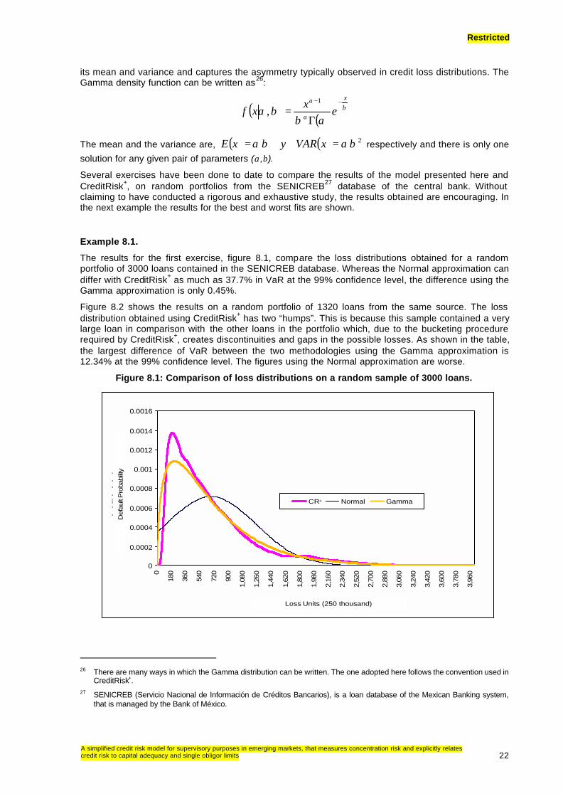
Example 8.1.

The results for the first exercise, figure 8.1, compare the loss distributions obtained for a random portfolio of 3000 loans contained in the SENICREB database. Whereas the Normal approximation can differ with CreditRisk+ as much as 37.7% in VaR at the 99% confidence level, the difference using the Gamma approximation is only 0.45%.

Figure 8.2 shows the results on a random portfolio of 1320 loans from the same source. The loss distribution obtained using CreditRisk+ has two “humps”. This is because this sample contained a very large loan in comparison with the other loans in the portfolio which, due to the bucketing procedure required by CreditRisk+, creates discontinuities and gaps in the possible losses. As shown in the table, the largest difference of VaR between the two methodologies using the Gamma approximation is 12.34% at the 99% confidence level. The figures using the Normal approximation are worse.

Figure 8.1: Comparison of loss distributions on a random sample of 3000 loans.

0

0.0002

0.0004

0.0006

0.0008

0.001

0.0012

0.0014

0.0016

0

180

360

540

720

900

1,08

0

1,26

0

1,44

0

1,62

0

1,80

0

1,98

0

2,16

0

2,34

0

2,52

0

2,70

0

2,88

0

3,06

0

3,24

0

3,42

0

3,60

0

3,78

0

3,96

0

unidades de pérdida (250 mil)

pro

bab

ilid

ad d

e im

pag

o

CR+ Normal Gama

Loss Units (250 thousand)

Def

ault

Pro

babi

lity

CR+ Normal Gamma

0

0.0002

0.0004

0.0006

0.0008

0.001

0.0012

0.0014

0.0016

0

180

360

540

720

900

1,08

0

1,26

0

1,44

0

1,62

0

1,80

0

1,98

0

2,16

0

2,34

0

2,52

0

2,70

0

2,88

0

3,06

0

3,24

0

3,42

0

3,60

0

3,78

0

3,96

0

unidades de pérdida (250 mil)

pro

bab

ilid

ad d

e im

pag

o

CR+ Normal Gama

Loss Units (250 thousand)

Def

ault

Pro

babi

lity

CR+ Normal GammaCR+ Normal Gamma

26 There are many ways in which the Gamma distribution can be written. The one adopted here follows the convention used in

CreditRisk+. 27 SENICREB (Servicio Nacional de Información de Créditos Bancarios), is a loan database of the Mexican Banking system,

that is managed by the Bank of México.

Restricted


Table 8.1: VaR comparative statistics for the sample.

VaR Confidence Level 0.95 0.975 0.99 0.995

CR+ 1,878 2,212 2,623 2,932

Normal 1,590 1,765 1,969 2,108

Gamma 1,770 2,120 2,577 2,919

Loss Distribution Statistics Mean Variance Std. Deviation alfa beta

CR+ 673 312,277 559 - -

Normal 674 310,116 557 - -

Gamma 674 310,116 557 1.46 460.27

Figure 8.2: Comparison of loss distributions on a random sample of 1320 loans.

0

0.0002

0.0004

0.0006

0.0008

0.001

0.0012

0.0014

0.0016

0 250 500 750 1000 1250 1500 1750 2000 2250 2500 2750 3000

CR+ Gamma Normal

Distribution VaR95 VaR97.5 VaR99 VaR99.5CreditRisk+ 1606 1790 2030 2190Gamma 1467 1618 1807 1942Normal 1405 1509 1630 1712

0

0.0002

0.0004

0.0006

0.0008

0.001

0.0012

0.0014

0.0016

0 250 500 750 1000 1250 1500 1750 2000 2250 2500 2750 30000

0.0002

0.0004

0.0006

0.0008

0.001

0.0012

0.0014

0.0016

0

0.0002

0.0004

0.0006

0.0008

0.001

0.0012

0.0014

0.0016

0 250 500 750 1000 1250 1500 1750 2000 2250 2500 2750 30000 250 500 750 1000 1250 1500 1750 2000 2250 2500 2750 3000

CR+ Gamma Normal

Distribution VaR95 VaR97.5 VaR99 VaR99.5CreditRisk+ 1606 1790 2030 21901606 1790 2030 2190Gamma 1467 1618 1807 19421467 1618 1807 1942Normal 1405 1509 1630 17121405 1509 1630 1712

It should be pointed out that not all of the exercises produced VaR differences where the model underestimated the results of CreditRisk+. Some of the random portfolios provided results where the opposite occurred using the Gamma approximation. In all of these cases the differences were small. §

It is not always the case that the VaR obtained by CyRCE is less than the corresponding VaR obtained using CreditRisk+. Although the preceding examples are interesting and serve to illustrate the kind of results obtained by both methods, they are far from being a rigorous comparative study. In particular, it is interesting to examine how the two methodologies behave, as the number of loans in the portfolio increases. In order to explore this behavior, a simulation experiment was done, taking random samples of portfolios of increasing numbers of loans, and their VaR was calculated by both methods, for different confidence levels.28 The results of the exercise are summarized in figure 8.3.

28 Thus, for each of the 23 sizes of portfolio, between 2,000 and 64,000 loans, 500 simulation runs were performed. Due to the

characteristics of the SENICREB database, sampling was done with replacement for the larger sizes.

Restricted


The number of loans in the portfolios shown on the x-axis, while the y-axis shows the average of the following statistic:

carteraladeValor

CaRVaRCreditRiskCyRCE +−

=∆

The curves in the graph represent the average differences in VaR relative to the value of the portfolio, for different confidence levels. The Gamma distribution was used for approximating the loss distribution obtained by CyRCE.

Figure 8.3. Comparison between CreditRisk + and CyRCE as the number of loans increases in the portfolio, for different confidence levels.

-4%

-3%

-2%

-1%

0%

1%

2%

0 5,000 10,000 15,000 20,000 25,000 30,000 35,000 40,000 45,000

Numberof Loans

LoanTotalRiskCreditVaRCyRCEVaR )( +-

95

97.5

98

99

99.5

ConfidenceLevel

-4%

-3%

-2%

-1%

0%

1%

2%

0 5,000 10,000 15,000 20,000 25,000 30,000 35,000 40,000 45,000

Numberof Loans



95

97.5

98

99

99.5

ConfidenceLevel

First, it is interesting to note that the average difference of VaR’s relative to the size of the portfolio decreases as the number of loans increases. This provides some empirical evidence that there is some sort of large numbers effect. Next, the graph shows that on average, the VaR obtained by CyRCE overestimates that obtained by CreditRisk+ for confidence levels below 98%, and underestimates them for higher confidence levels. Undoubtedly, this is due to the heavier tales of the loss distribution generated by CreditRisk+.§

9. Application of the model with limited portfolio information.

Any credit risk model requires two types of information; namely: A description of the loans in the portfolio, and the default behavior of the loans it contains. (i.e. default probabilities and correlations). The model presented here allows several options for performing calculations with limited information. Regardless of the quality of information available on default rates of loans in a portfolio, it is the authors’ experience that in the worse case, bankers have some idea of what these are, even if it is not available in some sort of systematized database. The estimation of default probabilities and correlations from default rates, is a topic in itself and will not be dealt with here. On the other hand, the difficulties of obtaining portfolio information is of particular relevance to regulators, and probably constitutes the largest stumbling block for effective credit risk supervision. Banks are reluctant to provide regulators with this information on an ongoing basis simply because of the huge quantities of data involved. Even if the data could be obtained in an appropriate and systematic way, it would be difficult to handle. Private banks with large portfolios would also benefit from reducing information requirements to run their models. We now address this issue.

Restricted


As seen in the derivation of the model, it is not strictly necessary to know the credit portfolios in detail. Given an adequate segmentation of the portfolio, the only information required by the model is:

a) The total value of the loans in each segment Vi.

b) Enough information about the loan distribution within each segment, which allows an estimate of its HHI.

c) Estimates of “pi”, “ρ i” and “ρ ij”.

In what follows, we will discuss how estimates of HHI can be obtained from some very basic statistics. Thus, suppose that the portfolio has been segmented into “h” segments. If for each segment one

knows the value of the segment Vi , and the value of the largest loan in each segment, "" *if , then

theorem 5.3 states that:

i

iii V

fH

*

)( =≤ θF ….(9.1)

Therefore, iiH θ=)(F , is an estimate of HHI for each segment, although perhaps a bit crude. In fact,

theorem 5.3 can be used to obtain a slightly tighter bound. To see this, remember that the largest concentration occurs when the portfolio has the following distribution as a proportion of its value “V”:

+=+=

=

=Nnk

nk

nk

f k

,...,2 ;01 ;

,...,2,1 ;

ε

θ

∑ =+= 1εθnf k

For this distribution,

H(F) = n?2 + ε2 = n?•θ + ε2 = (1-ε)? + ε2.

This expression is minimum when ε = 0.5?. Since it is practically imposible to have Duch a distribution in practice, if only the largest loan in each segment is known, one could argue that a good bound on HHI is:

H(F) < θ(1-0.5θ) ……………(9.2)

If the number of loans per segment Ni is known, as well as the average size loan if and the variante 2iσ , then HHI can be obtained. To see this, first note that iii fNV = is the value of each segment

and ∑=

=h

iiVV

1

is the value of the portfolio. Then, by the definition of variance:

( )( ) ( )[ ] ( )

( )( )( ) ( )

( )( )

( )( )

( )( )

−−

=

−−

=

−−

=+−−

=−

−=

∑

∑∑∑

ii

i

i

k iii

ik

i

ii

kii

ik

iii

ii

kii

ik

ik

ii

ki

ik

i

NH

NV

NfN

fN

fN

fNffNN

fNffff

NN

ff

1)(

11

1

12

11

1

2

2

22

22

2

222

2

2

F

σ

Solving for HHI one obtains:

Restricted


( )

ii

i

i

ii NfN

NH

11)(

2

2 +

−=

σF ….. (9.3)

Now, having estimates of HHI for each segment, one can obtain the HHI of the whole portfolio as follows:

∑∑ ∑∑∑== == =

===

h

ii

ih

i

N

k i

kii

h

i

N

kki H

VV

V

fV

Vf

VH

ii

1

2

1 12

2,2

21 1

2,2

)(11

)( FF (9.4)

Note that (9.3) and (9.4) are exact values for the concentration indices, and that they can be obtained with very limited information.

9. Systemic Credit Risk Analysis of the Mexican Banking System.

Using the SENICREB database, the model is currently being used to analyze the credit risk profile, and capital adequacy of the 20 banks of the Mexican financial system. The results are presented to the board of governors of the Central Bank on a monthly basis. In the exercise presented here for illustrative purposes, we assume that the underlying loss distribution is normal and VaR computations are for a monthly horizon at the 2.5% confidence level. Due to the centralization that characterizes the Mexican economy, it is difficult to segment by geographical region. As a starting point, the loan portfolio of the system has been segmented by bank and economic activity. Loans rated by one or more of the major rating agencies form a separate segment, because there are relatively few rated loans so the observed history of their default behavior is insufficient for default probability and correlation estimation. Fortunately, the rating agencies themselves provide good estimates of these parameters.

Figure 7.1 shows how the loan market was distributed among the major banks in Mexico at the end of March 2002. Two banks have 48% of the market, and 91% of all loans are held by seven banks.

Figure 7.1: Distribution of the loan portfolio by major banks. March 2002.

Loan portfolio of the System = 343,357

82,05625%

33,3589%

81,55124%

21,0386%

27,7178.1%

30,7008.7%

32,2329% 34,704

10%

82,05625%

33,3589%

81,55124%

21,0386%

27,7178.1%

30,7008.7%

32,2329% 34,704

10%

* Millions of pesos.

Restricted


Figure 7.2 shows the distribution of the loan portfolio of the banking system segmented by economic activity. In the graph we see that the largest segment is represented by mortgage and consumer loans, followed by financial services and so on.

Figure 7.2: Distribution of the loan portfolio by economic activity. March 2002.

Figure 7.3, shows the variation over time of VaR, default probabilities, HHI concentration index, covariation index and VaR relative to economic capital for the Banking system.

Figure 7.3: Evolution of the Risk Profile of the Mexican Banking System.

27,1

66

33,0

58

27,7

58

30,8

49

35,5

42

34,5

30

32,7

52

34,3

93

35,2

35

38,0

35

36,1

07

28,6

65

29,5

37

27,3

07 36,0

13

37,6

88

35,3

19

33,9

23

31,7

04

0.0%

0.2%

0.4%

0.6%

0.8%

1.0%

1.2%

1.4%

p /

IHH

0

5,000

10,000

15,000

20,000

25,000

30,000

35,000

40,000

VaR

95 (millio

ns o

fpesos)

Mar Jun Sep Dec Jan Feb Mar Apr May Jun Jul Aug Sep Oct Nov Dec Jan Feb Mar

2000 2001 2002

p 1.2% 1.3% 1.3% 1.1% 1.1% 1.1% 1.1% 1.1% 1.1% 1.1% 1.1% 1.3% 1.1% 1.1% 1.1% 1.1% 1.2% 1.2% 1.2%

IHH 1.1% 0.7% 0.7% 0.7% 0.6% 0.6% 0.7% 0.6% 0.7% 0.6% 0.6% 0.6% 0.6% 0.6% 0.7% 0.8% 0.7% 0.8% 0.9%

23%30%

22% 25% 29% 28% 26% 27% 26% 28% 27%21% 22% 20%

27% 28% 27% 25% 23%VaR/Economic

Capital

1.6

2.61.9 2.2

2.9 2.9 2.8 3.0 2.63.9 3.4

1.9 2.1 1.72.7 2.7 2.4 2.0 1.6

VarianceCovariance

Index

VaR95 Herfindahl IndexDefault Probability

27,1

66

33,0

58

27,7

58

30,8

49

35,5

42

34,5

30

32,7

52

34,3

93

35,2

35

38,0

35

36,1

07

28,6

65

29,5

37

27,3

07 36,0

13

37,6

88

35,3

19

33,9

23

31,7

04

0.0%

0.2%

0.4%

0.6%

0.8%

1.0%

1.2%

1.4%

p /

IHH

0

5,000

10,000

15,000

20,000

25,000

30,000

35,000

40,000

VaR

95 (millio

ns o

fpesos)

Mar Jun Sep Dec Jan Feb Mar Apr May Jun Jul Aug Sep Oct Nov Dec Jan Feb Mar

2000 2001 2002

p 1.2% 1.3% 1.3% 1.1% 1.1% 1.1% 1.1% 1.1% 1.1% 1.1% 1.1% 1.3% 1.1% 1.1% 1.1% 1.1% 1.2% 1.2% 1.2%

IHH 1.1% 0.7% 0.7% 0.7% 0.6% 0.6% 0.7% 0.6% 0.7% 0.6% 0.6% 0.6% 0.6% 0.6% 0.7% 0.8% 0.7% 0.8% 0.9%

23%30%

22% 25% 29% 28% 26% 27% 26% 28% 27%21% 22% 20%

27% 28% 27% 25% 23%VaR/Economic

Capital

1.6

2.61.9 2.2

2.9 2.9 2.8 3.0 2.63.9 3.4

1.9 2.1 1.72.7 2.7 2.4 2.0 1.6

VarianceCovariance

Index 1.6

2.61.9 2.2

2.9 2.9 2.8 3.0 2.63.9 3.4

1.9 2.1 1.72.7 2.7 2.4 2.0 1.6

VarianceCovariance

Index

VaR95VaR95 Herfindahl IndexDefault Probability

Non-rated loans (85%)

0

10,000

20,000

30,000

40,000

50,000

60,000

70,000

80,000

90,000

0%

5%

10%

15%

20%

25%

Rated loans* (15%)

0

10,000

20,000

30,000

40,000

50,000

60,000

70,000

80,000

90,000

0%

5%

10%

15%

20%

25%

MDP

Total Loan Portfolio : 343,357 MDP

Mo

rtg

age

& C

on

sum

ptio

n

Fin

anci

al S

ervi

ces

Pro

fess

ion

al S

ervi

ces

Co

mm

erce

of P

rod

uct

s

Co

nst

ruct

ion

Co

mm

. & T

ran

sp.

I. M

etal

s &

Met

allic

Pro

d.

Co

mm

erce

of R

aw M

ater

ials

I. F

oo

d In

du

stry

I. M

ach

iner

y &

Eq

uip

.

I. N

on-M

etal

lic M

in. &

Pla

stic

s

Hot

els,

Res

t. &

Rec

r. S

ervi

ces

I. W

oo

d &

Pap

er In

d.

Oth

er In

dust

ries

I. T

exti

le In

d.

I. C

hem

ical

Ind

.

Agr

icul

ture

Oth

ers

Liv

esto

ck

I. E

xtra

ctiv

e In

d.

So

cial

& C

om

mu

n.

Ser

vice

s

Non-rated loans (85%)

0

10,000

20,000

30,000

40,000

50,000

60,000

70,000

80,000

90,000

0%

5%

10%

15%

20%

25%

Rated loans* (15%)

0

10,000

20,000

30,000

40,000

50,000

60,000

70,000

80,000

90,000

0%

5%

10%

15%

20%

25%

MDP

Total Loan Portfolio : 343,357 MDP

Mo

rtg

age

& C

on

sum

ptio

n

Fin

anci

al S

ervi

ces

Pro

fess

ion

al S

ervi

ces

Co

mm

erce

of P

rod

uct

s

Co

nst

ruct

ion

Co

mm

. & T

ran

sp.

I. M

etal

s &

Met

allic

Pro

d.

Co

mm

erce

of R

aw M

ater

ials

I. F

oo

d In

du

stry

I. M

ach

iner

y &

Eq

uip

.

I. N

on-M

etal

lic M

in. &

Pla

stic

s

Hot

els,

Res

t. &

Rec

r. S

ervi

ces

I. W

oo

d &

Pap

er In

d.

Oth

er In

dust

ries

I. T

exti

le In

d.

I. C

hem

ical

Ind

.

Agr

icul

ture

Oth

ers

Liv

esto

ck

I. E

xtra

ctiv

e In

d.

So

cial

& C

om

mu

n.

Ser

vice

s

* Rated by Standard & Poor’s , Moody’s y Fitch

Restricted


This graph summarizes how systemic VaR responds to the main risk drivers, and provides a first indication on how well the banking system is capitalized relative to the level of risk taken.

Figure 7.4 shows the concentration of risk in the system. Banks are sorted out by their contribution to the overall VaR of the system, and arranged from largest to smallest. A Lorenz curve is constructed so that the amount of risk concentrated in a specific number of banks can be seen. The bars in the graph represent the ratio of each banks’ VaR relative to its Net Capital. The horizontal line is the average VaR to net capital ratio for the system, so that one can see the relative position of each bank with respect to the system. Thus, 80% of the risk is concentrated in five banks and the third of these has VaR to net capital ratio of 64% which is a relatively high when compared to 23% average of the system.

Figure 7.4: Individual Banks Contribution to Systemic Risk: March 2002

Figure 7.5: Contribution to System Risk by Economic Activity: Marzo de 2002

Figure 7.5, shows the contribution of the individual segments of economic activity. Most of the risk is in consumer and mortgage loans, followed by financial services. Note that construction and

/EC

1% 0% 1%2%5%2%6%24%

38%

20%19%13%

63%

11%

45%

14%39%

64% 38%

32%24% 22% 27% 22% 18% 20% 18%

71%

62%

26%

50%

80%

0%

10%

20%

30%

40%

50%

60%

70%

80%

90%

100%

100%98%

B1

B2

B3

B4

B5

B6

B7

B8

B9

B10

B11

B12

B13

B14

B15

B16

B17

B18

B19

B20

B21

B22

B23

B24

B25

B26

B27

1% 0% 1%2%5%2%6%24%

38%

20%19%13%

63%

11%

45%

14%39%

64% 38%

32%24% 22% 27% 22% 18% 20% 18%

71%

62%

26%

50%

80%

0%

10%

20%

30%

40%

50%

60%

70%

80%

90%

100%

100%98%

B1

B2

B3

B4

B5

B6

B7

B8

B9

B10

B11

B12

B13

B14

B15

B16

B17

B18

B19

B20

B21

B22

B23

B24

B25

B26

B27

VaR95 VaR95 acumulated VaR95 /EC average: 23% VaR95 VaR95 VaR95 VaR95

VaR95/System VaR VaR95 acumulate

4% 3% 3% 3% 2% 2% 2% 1% 1% 1% 1%

6% 6% 5%5%

26%

9%7% 7%

4%

98%

83%

0%

5%

10%

15%

20%

25%

30%

0%10%

20%30%40%50%

60%70%80%

90%100%

Mo

rtg

age

& C

on

sum

pti

on

Fin

anci

al S

ervi

ces

Co

nst

ruct

ion

Pro

fess

ion

al S

ervi

ces

I. M

etal

s &

Met

allic

Pro

d.

Co

mm

. & T

ran

sp.

Com

mer

ce o

f Raw

Mat

eria

ls

I. W

oo

d &

Pap

er In

d.

Oth

er I

nd

ust

ries

Co

mm

erce

of P

rod

uct

s

I. M

aqu

iner

y&

Eq

uip

.

I. Fo

od In

dust

ry

Ho

tels

, Res

t. &

Rec

r. S

ervi

ces

I. T

exti

le In

d.

I. N

on

-Met

allic

Min

. & P

last

ics

I. E

xtra

ctiv

e In

d.

Liv

esto

ck

I. C

hem

ical

Ind

.

Agr

icul

ture

Soc

ial &

Co

mm

un

. Ser

vice

s

Oth

ersVaR95/System VaR VaR95 acumulateVaR95/System VaR VaR95 acumulateVaR95 acumulate

4% 3% 3% 3% 2% 2% 2% 1% 1% 1% 1%

6% 6% 5%5%

26%

9%7% 7%

4%

98%

83%

0%

5%

10%

15%

20%

25%

30%

0%10%

20%30%40%50%

60%70%80%

90%100%

Mo

rtg

age

& C

on

sum

pti

on

Fin

anci

al S

ervi

ces

Co

nst

ruct

ion

Pro

fess

ion

al S

ervi

ces

I. M

etal

s &

Met

allic

Pro

d.

Co

mm

. & T

ran

sp.

Com

mer

ce o

f Raw

Mat

eria

ls

I. W

oo

d &

Pap

er In

d.

Oth

er I

nd

ust

ries

Co

mm

erce

of P

rod

uct

s

I. M

aqu

iner

y&

Eq

uip

.

I. Fo

od In

dust

ry

Ho

tels

, Res

t. &

Rec

r. S

ervi

ces

I. T

exti

le In

d.

I. N

on

-Met

allic

Min

. & P

last

ics

I. E

xtra

ctiv

e In

d.

Liv

esto

ck

I. C

hem

ical

Ind

.

Agr

icul

ture

Soc

ial &

Co

mm

un

. Ser

vice

s

Oth

ers

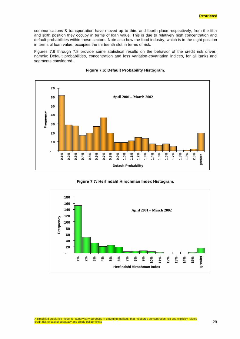
Restricted


communications & transportation have moved up to third and fourth place respectively, from the fifth and sixth position they occupy in terms of loan value. This is due to relatively high concentration and default probabilities within these sectors. Note also how the food industry, which is in the eight position in terms of loan value, occupies the thirteenth slot in terms of risk.

Figures 7.6 through 7.8 provide some statistical results on the behavior of the credit risk driver; namely: Default probabilities, concentration and loss variation-covariation indices, for all banks and segments considered.

Figure 7.6: Default Probability Histogram.

Figure 7.7: Herfindahl Hirschman Index Histogram.

-

20

40

60

80

100

120

140

160

180

1% 2% 3% 4% 5% 6% 7% 8% 9% 10%

11%

12%

13%

14%

15%

gre

ater

Herfindahl Hirschman Index

Fre

qu

ency

April 2001 – March 2002

-

10

20

30

40

50

60

70

0.1%

0.2%

0.3%

0.4%

0.5%

0.6%

0.7%

0.8%

0.9%

1.0%

1.1%

1.2%

1.3%

1.4%

1.5%

1.6%

1.7%

1.8%

1.9%

2.0%

gre

ater

Default Probability

Fre

qu

ency


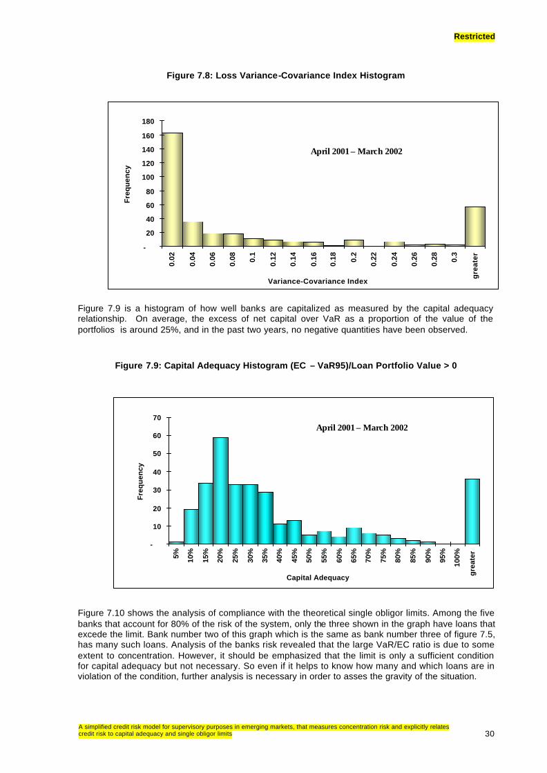
Restricted


Figure 7.8: Loss Variance-Covariance Index Histogram

Figure 7.9 is a histogram of how well banks are capitalized as measured by the capital adequacy relationship. On average, the excess of net capital over VaR as a proportion of the value of the portfolios is around 25%, and in the past two years, no negative quantities have been observed.

Figure 7.9: Capital Adequacy Histogram (EC – VaR95)/Loan Portfolio Value > 0

Figure 7.10 shows the analysis of compliance with the theoretical single obligor limits. Among the five banks that account for 80% of the risk of the system, only the three shown in the graph have loans that excede the limit. Bank number two of this graph which is the same as bank number three of figure 7.5, has many such loans. Analysis of the banks risk revealed that the large VaR/EC ratio is due to some extent to concentration. However, it should be emphasized that the limit is only a sufficient condition for capital adequacy but not necessary. So even if it helps to know how many and which loans are in violation of the condition, further analysis is necessary in order to asses the gravity of the situation.

-

20

40

60

80

100

120

140

160

180

0.02

0.04

0.06

0.08 0.

1

0.12

0.14

0.16

0.18 0.

2

0.22

0.24

0.26

0.28 0.

3

gre

ater

Variance-Covariance Index

Fre

qu

ency


-

10

20

30

40

50

60

70

5% 10%

15%

20%

25%

30%

35%

40%

45%

50%

55%

60%

65%

70%

75%

80%

85%

90%

95%

100%

gre

ater

Capital Adequacy

Fre

qu

ency


Restricted


Figure 7.10: Loans that exceed single obligor limits in 5 major Banks. March 2002

These graphs give a good idea of the type of analysis that is possible using the model. The same amount of detail is obtained for every bank in the system, permitting deeper analysis of their situation.§

9. Concluding remarks.

The results obtained are very appealing for managing credit risk, since they provide explicit formulas to measure risk and permit a precise quantification of the policy actions that should be adopted in order to maintain capital adequacy. If default or recovery rates change, or concentration along a particular segment is excessive, the relations can be used to determine the adjustments to the capitalization ratio and/or concentration composition of the portfolio that would reestablish capital adequacy. If banks have control over default or recovery rates to some degree, these can be part of the management instruments that can be used to maintain capital adequacy.

Since single obligor limits and HHI are related to concentration, and the measures are subject to the same bound, either one can be used as a policy instrument. In fact, both measures can be used in conjunction. Whereas the single obligor limit is easy to implement and supervise, it may lead to overly constrained loan distributions. On the other hand, although Herfindahls index allows more flexibility in the configuration of the portfolio, it is difficult to implement throughout the organization. For example, if a greedy bank manager decides to grant a loan exceeding his limit, the gravity of the transgression may be assessed using HHI. It may be that apart from misbehavior, the infraction is not serious in terms of risk.

It is clear that default probability distributions as well as recovery rates exhibit random behaviors through time, depending economic and financial factors. As opposed to market risk, where risk factors can be modeled using continuous processes, because loan defaults are discrete events in time, default behavior in a certain group can also change in pronounced discrete jumps. This is one reason why it is difficult to establish ex-ante concentration. Under different economic conditions, default probabilities and correlations can increase for a certain group of debtors, which otherwise appeared to be unrelated. For example a group of mortgage loans to employees of a large company that goes bankrupt. Since the model can handle arbitrary segmentations of the portfolio, and it is relatively simple to stress particular segments and analyze the consequences, it provides a means for detecting ex-ante concentration.

0%

50%

100%

150%

200%

250%

300%

350%

B1

B2

B3

Loans that exceed the obligor limit

Su

rplu

s p

erce

nta

ge

reg

ard

ing

th

e si

ng

le

ob

ligo

r lim

it o

f th

e B

ank

Restricted


There is no reason why default probabilities cannot be made to depend on risk factors and credit drivers through logit models as in Credit Portfolio View, or as linear combinations of these factors as proposed by Kreinin and Rosen. Since these are determined exogenously, the results can be imbedded in simulation models which generate scenarios of trajectories of these variables through time that exhibit the discontinuities typical of default related events. From these, one can obtain stressed loss distributions and all the related statistics for each segment and the portfolio. This type of experiment may be what is needed to set the proper policy on the capitalization ratio and single obligor limits. Notice that since the simulation process in this case is for only a few variables, it can be done very efficiently.

Whatever the dynamics, it is always possible to make the necessary adjustments through time by monitoring only a few variables.

Restricted


APENDIX A

Variance-Covariance Matrix

Example 6.1.

Table B.2: M1

Table B.3: 21T

12 CC =

Table B.4: 31T

13 CC =

1 2 3 4 5 6 7 81 0.0162 0.0050 0.0050 0.0060 0.0060 0.0082 0.0082 0.01052 0.0050 0.0475 0.0086 0.0103 0.0103 0.0140 0.0140 0.01803 0.0050 0.0086 0.0475 0.0103 0.0103 0.0140 0.0140 0.01804 0.0060 0.0103 0.0103 0.0694 0.0125 0.0169 0.0169 0.02175 0.0060 0.0103 0.0103 0.0125 0.0694 0.0169 0.0169 0.02176 0.0082 0.0140 0.0140 0.0169 0.0169 0.1275 0.0230 0.02957 0.0082 0.0140 0.0140 0.0169 0.0169 0.0230 0.1275 0.02958 0.0105 0.0180 0.0180 0.0217 0.0217 0.0295 0.0295 0.2100

1 2 3 4 5 6 7 89 0.0063 0.0108 0.0108 0.0130 0.0130 0.0177 0.0177 0.022710 0.0081 0.0138 0.0138 0.0166 0.0166 0.0226 0.0226 0.029011 0.0081 0.0138 0.0138 0.0166 0.0166 0.0226 0.0226 0.029012 0.0111 0.0190 0.0190 0.0229 0.0229 0.0311 0.0311 0.039913 0.0111 0.0190 0.0190 0.0229 0.0229 0.0311 0.0311 0.039914 0.0132 0.0226 0.0226 0.0273 0.0273 0.0370 0.0370 0.047515 0.0169 0.0290 0.0290 0.0350 0.0350 0.0475 0.0475 0.060916 0.0169 0.0290 0.0290 0.0350 0.0350 0.0475 0.0475 0.0609

1 2 3 4 5 6 7 817 0.0039 0.0067 0.0067 0.0081 0.0081 0.0109 0.0109 0.014018 0.0052 0.0089 0.0089 0.0108 0.0108 0.0146 0.0146 0.018819 0.0067 0.0114 0.0114 0.0138 0.0138 0.0187 0.0187 0.024020 0.0081 0.0138 0.0138 0.0167 0.0167 0.0226 0.0226 0.029021 0.0092 0.0157 0.0157 0.0190 0.0190 0.0257 0.0257 0.033022 0.0109 0.0187 0.0187 0.0226 0.0226 0.0306 0.0306 0.039323 0.0140 0.0240 0.0240 0.0290 0.0290 0.0393 0.0393 0.050424 0.0140 0.0240 0.0240 0.0290 0.0290 0.0393 0.0393 0.050425 0.0140 0.0240 0.0240 0.0290 0.0290 0.0393 0.0393 0.0504

Restricted


Table B.5: M2

Table B.6: 23T

32 CC =

Table B.7: M3

9 10 11 12 13 14 15 169 0.0291 0.0086 0.0086 0.0118 0.0118 0.0140 0.0180 0.0180

10 0.0086 0.0475 0.0109 0.0150 0.0150 0.0179 0.0230 0.023011 0.0086 0.0109 0.0475 0.0150 0.0150 0.0179 0.0230 0.023012 0.0118 0.0150 0.0150 0.0900 0.0207 0.0246 0.0316 0.031613 0.0118 0.0150 0.0150 0.0207 0.0900 0.0246 0.0316 0.031614 0.0140 0.0179 0.0179 0.0246 0.0246 0.1275 0.0376 0.037615 0.0180 0.0230 0.0230 0.0316 0.0316 0.0376 0.2100 0.048316 0.0180 0.0230 0.0230 0.0316 0.0316 0.0376 0.0483 0.2100

17 18 19 20 21 22 23 24 259 0.0070 0.0093 0.0119 0.0144 0.0164 0.0195 0.0250 0.0250 0.025010 0.0089 0.0119 0.0152 0.0184 0.0209 0.0249 0.0320 0.0320 0.032011 0.0089 0.0119 0.0152 0.0184 0.0209 0.0249 0.0320 0.0320 0.032012 0.0122 0.0164 0.0209 0.0253 0.0288 0.0343 0.0440 0.0440 0.044013 0.0122 0.0164 0.0209 0.0253 0.0288 0.0343 0.0440 0.0440 0.044014 0.0146 0.0195 0.0249 0.0301 0.0343 0.0408 0.0524 0.0524 0.052415 0.0187 0.0250 0.0320 0.0386 0.0440 0.0524 0.0672 0.0672 0.067216 0.0187 0.0250 0.0320 0.0386 0.0440 0.0524 0.0672 0.0672 0.0672

17 18 19 20 21 22 23 24 2517 0.0162 0.0093 0.0119 0.0144 0.0164 0.0196 0.0251 0.0251 0.025118 0.0093 0.0291 0.0160 0.0193 0.0220 0.0262 0.0336 0.0336 0.033619 0.0119 0.0160 0.0475 0.0247 0.0281 0.0335 0.0429 0.0429 0.042920 0.0144 0.0193 0.0247 0.0694 0.0340 0.0404 0.0519 0.0519 0.051921 0.0164 0.0220 0.0281 0.0340 0.0900 0.0461 0.0591 0.0591 0.059122 0.0196 0.0262 0.0335 0.0404 0.0461 0.1275 0.0704 0.0704 0.070423 0.0251 0.0336 0.0429 0.0519 0.0591 0.0704 0.2100 0.0903 0.090324 0.0251 0.0336 0.0429 0.0519 0.0591 0.0704 0.0903 0.2100 0.090325 0.0251 0.0336 0.0429 0.0519 0.0591 0.0704 0.0903 0.0903 0.2100

Restricted


References.

Adelman, M. A. 1969. Comment on the “H” Concentration Measure as a Numbers-Equivalent . Review of Economics and Statistics, February, pp. 99-101.

Altman Edward I., and Anthony Saunders 1998. Credit risk measurement: Developement over the last 20 years. Journal of Banking & Finance 21 (1998) 1721-1742.

Crouhy, Michel, Dan Galai and Robert Mark: A comparative analysis of current credit risk models. Journal of Banking and Finance 24 (2000) pp. 59-117.

Basle Committee on Banking Supervision, 1999. Credit Risk Modeling: Current Practices and Applications.

Bennet, P. 1984. Applying Portfolio Theory to Global Bank Lending. Journal of Banking and Finance.

Caouette, John B., Edward I. Altman y Paul Narayanan 1998. Managing Credit Risk: The next great challenge. Ed. John Wiley & Sons, Inc.

Coopers and Lybrand. 1993. Growth and Diversification: Are the Benefits Always There? In Mortgage Banking, edited by J. Lederman. Chicago: Probus Publishing Company.

Cowell, Frank A., Measuring Inequality 2nd edition. LSE Handbooks in Economics, Prentice Hall/Harvester Wheatsheaf, 1995.

Credit Risk + : Credit Suisse Financial Products, New York, N.Y. 1996.

CreditMetricsTM: Technical document, April 2nd, 1997.

De Groot, Morris H., Probabilidad y Estadística, Addison-Wesley Iberoamericana, Wilmington Delaware. 1988.

Encaoua, David and Jacquemin, Alexis. 1980. Degree of monopoly, indices of concentration and threat of entry. International, Economic Review 21.

Finger, Christopher C.: Sticks and Stones, The RiskMetrics Group. 1998

Gordy, Michael B. A comparative Anatomy of Credit Risk Models. Journal of Banking and Finance, vol 24, 2000, pp. 119-149.

Kealhofer, S. Portfolio Management of Default Risk. KMV Corporation, 1998.(Revised.)

Kealhofer, S. Modeling Default Risk . KMV Corporation, 1999 (Revised.)

Kelly Jr. W.A. 1981. A Generalized Interpretation of the Herfindahl Index. Southern Economic Journal, 48(1) pp. 50-57.

Lambert, Peter J. 1993. The Distribution and Redistribution of Income, Ed. Manchester University Press.

Márquez Diez-Canedo, Javier, 2002. Capital Adequacy and Credit Risk in Bank Loan Portfolios: A default model that relates capital adequacy to credit risk, measures concentration, and obtains single obligor limits. Economia, Societa’ e Istituzioni, Anno XIV/n° 1 Gennaio – Aprile 2002.

Márquez Diez-Canedo, Javier 1987. Fundamentos de Teoría de Optimización, Editorial Limusa S.A. de C.V.

Markowitz, H. 1959. Portfolio Selection: Efficient Diversification of Investments. New York: John Wiley & Sons.

Mason, S. P. 1995. The allocation of Risk. In The Global Financial System. Boston: Harvard Business School Press.

Merton, R. C. On the pricing of corporate debt: The risk structure of interest rates .”Journal of Finance 29, pp. 449-470, 1974.

Mirsky, L. An introduction to linear algebra. Dover Publications, Inc.1990

Restricted


Moody’s Investors Service. 1991. Rating Cash Flow Transactions Backed by Corporate Debt. Moody’s Special Report. April.

Nash, Stephen G. and Ariela Sofer 1996. Linear and Nonlinear Programming, The McGraw-Hill Companies, Inc.

Neckell, Pamela, W. Perraudin and S. Varotto: Stability of Rating Transitions. Journal of Banking and Finance, vol. 24, pp. 203-227, 2000.

Shy, Oz. 1995. Industrial Organization: Theory and Applications. The MIT press.

Sleuwaegen, Leo E., Raymond R. De Bondt, and Wim V. Dehandschuter. The Herfindahl index and concentration ratios revisited. The Antitrust Bulletin/Fall 1989.

Theil, Henri 1967. Information Theory, Ed. North Holland Publishing Co.

Tirole, Jean. 1995. The Theory of Industrial Organization. M. I. T. Press.

Weinstock, David S. Some little-known properties of the Herfindahl-Hirschman Index: Problems of Translation and Specification. The Antitrust Bulletin/ Winter 1984.

Wilson, Thomas C. Portfolio Credit Risk (I). Risk magazine, 10(9) September 1997.

Wilson, Thomas C. Portfolio Credit Risk (II). Risk magazine, 10(10) October 1997.

Documents

A simplified credit risk model for supervisory purposes in ... · A simplified credit risk model for supervisory purposes in emerging markets, ... distribution, so that the ... default