Abstract

Image denoising, particularly Gaussian denoising, has

achieved continuous success in the past decades. Although

deep convolutional neural networks (CNNs) are also shown leading high-performance in Gaussian denoising just as in

many other computer vision tasks, they are not competitive

at all on real noisy photographs to representative classical

methods such as BM3D and WNNM. In this paper, a simple

yet robust method is proposed to improve the effectiveness

and practicability of deep denoising models. In view of the

difference between real-world noise in camera systems and

additive white Gaussian noise (AWGN), the model learning

has exploited clean-noisy image pairs newly produced built

on a generalized signal dependent noise model. During the

model inference, the proposed denoising model is not only blind to the noise type but also to the noise level. Meanwhile,

in order to separate the noise from image content as full as

possible, a new convolutional architecture is advocated for

such a blind denoising task where a kind of lifting residual

modules is specifically proposed for discriminative feature

extraction. Experimental results on both simulated and real

noisy images demonstrate that the proposed blind denoiser

achieves fairly competitive or even better performance than

state-of-the-art algorithms in terms of both quantitative and

qualitative assessment. The codes of the proposed method

are available at https://github.com/zhaohengyuan1/SDNet.

1. Introduction

Image denoising is a fundamental problem in the fields

of image processing and computer vision. Classical

algorithms generally emphasize on the properties of natural

images and noise by exploiting hand-engineered and

analytical features. While with the rising popularity of the

convolutional neural networks (CNNs), modern denoising algorithms often learn a mapping from noisy images to their

counterpart noise-free versions in the framework of deep

supervised learning. In a typical denoising setting with

additive white Gaussian noise (AWGN), deep denoisers

have achieved significant success due to their advanced

(b) Noisy

(a) Real noisy image from [7] (c) DnCNN [2]

(d) WNNM [6] (e) CBM3D [5] (f) Ours

Figure 1: (a) A test image from the real noisy image dataset [7]. A local patch of the noisy and denoised image by each approach is shown around the test image. (b) Noisy patch, (c) DnCNN [2] (PSNR = 34.08 dB), (d) WNNM [6] (PSNR = 38.68 dB), (e) CBM3D [5] (PSNR = 39.72 dB), (f) Our SDNet (PSNR = 39.94 dB).

capabilities of representing complex properties of images

and noise. However, as turning to real noisy images, the

state-of-the-art deep denoising models for AWGN, e.g.,

TNRD [1] and DnCNN [2], are usually shown [3] inferior

performance to classical prior-based algorithms, e.g.,

BM3D [4], CBM3D [5] and WNNM [6]. The apparent

reason to such discrepancy is that Gaussian noise is largely

deviated from the real ones coming from five major sources

in camera systems including photon shot noise, dark current,

readout noise, fixed pattern noise and quantization noise. It

is thus required to formulate denoising of real photographs as a totally blind estimation problem. In practice, neither the

noise type nor the level is available in advance, which poses

a great challenge to both training and generalization of deep

CNNs. Figure 1 provides a denoising example from the real

A Simple and Robust Deep Convolutional Approach to Blind Image Denoising

Hengyuan Zhao1, Wenze Shao1, Bingkun Bao1, Haibo Li2

1Nanjing University of Posts and Telecommunications

2KTH Royal Institute of Technology hubylidayuan@gmail.com, shaowenze@njupt.edu.cn, bingkunbao@njupt.edu.cn,

haiboli@kth.se

noisy image dataset in [7], demonstrating that our proposed

deep method is a more appropriate candidate for real image

blind denoising.

Our Contributions. This paper presents a simple yet

robust method so as to improve the effectiveness

and practicability of deep denoising models. State-of-the-

art results are shown on simulated noisy images as well as

realistic noisy datasets. Two core considerations as

formulating blind denoising are that, on the one hand, the

noise model for preparing training images should not be

camera-specific; on the other hand, the blind deep denoiser should be applicable to distinct cameras

with varied settings while free of the need to estimate noise

level. According to the guideline, this paper generates a

new set of clean-noisy image pairs via use of a generalized

signal dependent noise model given a certain parameter

setting so as to better match the physics of real-world image

formation. It is discovered that, such a choice as above is

demonstrated feasible and applicable to denoising of real

photographs in spite of its blindness to the camera image

signal processing pipeline. The simplicity of the proposed

deep convolutional architecture for denoising is another highlight of the paper. It does not exploit the local statistics

or non-local similarity of natural images as in previous

strategies [4, 5, 6, 7, 8, 9, 10, 11, 12, 13, 14], while

emphasizes separating the noise from image content via a

direct fully end-to-end residual learning strategy wherein

seven lifting residual modules are involved. We note that,

our architecture, dubbed as SDNet, is inspired by the

networks suggested in [15], [16], [17], while with the

particular concentration in this paper on the discriminative

feature extraction for removing real-world camera noise.

To the best of our knowledge, SDNet is the first one

using the generalized signal dependent noise model [18] for stage- wise blind denoising of real photographs. Its whole

network architecture is provided in Figure 2. The main

contributions and highlights of this work can be

summarized as following which are four-fold:

1. We demonstrate that blind denoising of real photographs

can be made workable to a large degree by exploiting the

generalized signal dependent noise model for generating

pairs of clean-noisy training images.

2. SDNet is a fully end-to-end convolutional residual neural

network model for realistic color image denoising trained

without need of any hand-crafted priors or additional real noisy photographs (along with nearly noise-free images) for

data augmentation.

3. The core spirit of SDNet is to separate noise from image

content in stages and each stage contributes to the desired

overall noise map, whose prediction precision is ensured

largely by integrating our lifted residual modules and the

shortcut connections.

4. Experiments on both simulated and realistic noisy images

demonstrate that SDNet could achieve fairly competitive or

even better performance than state-of-the-art denoisers in

terms of both quantitative and qualitative assessment.

2. Related Work

AWGN Denoising. As one of the most fundamental image

processing problems, AWGN denoising has undergone fast

development ranging from classic variational, PDE,

wavelet, and stochastic algorithms [19, 20] to modern

nonparametric, self-similarity-driven techniques, e.g., non-

local means [21], BM3D [4]. They are all hand-engineered

methods, and the modern ones are demonstrated more

powerful in the model capacity and expressiveness for AWGN denoising. Another technical route for AWGN

denoising is data-driven, which concentrates on image

representation where either the patch sparsity or local

statistical regularities are to be learned, e.g., K-SVD [14,

22], Fields-of-Experts [23]. A non-local sparse modeling

idea is also advocated in [6, 8], and WNNM [6] is one of

the most representative methods. Nowadays, with the

prosperity of deep CNNs, single image AWGN denoising

is witnessing another round of fast development. DnCNN

[2] is the first deep denoiser outperforming the state-of-the-

art traditional methods such as BM3D [4], which is a 17-layer and fully end-to-end convolutional neural model to

learn the residual noise map assuming a certain noise

variance. Other recent CNN-based methods including

FFDNet [24], RED30 [16], MemNet [25], BM3D-Net [26]

and MWCNN [27] are also developed to solve the AWGN

denoising problem. For example, FFDNet [24] proposes a

flexible single network to deal with noisy images in various

noise levels. The network takes both the noise map and

noisy image as input and hence is more advanced than

DnCNN [2]. In addition, the dilated convolution operators

are exploited in FFDNet for detailed feature extraction.

Real Image Denoising. Because AWGN deviates from the noise greatly emerging in the practical camera image signal

processing pipeline, a few more recent efforts work towards

the real image denoising problem. And, it is discovered that

[3] state-of-the-art deep image denoisers, e.g., DnCNN, are

not competitive at all to BM3D and WNNM. To capture the

noise characteristics in real camera photographs, a common

strategy is to model them via the joint Gaussian-Poissonian

distribution [28]. In [29] the non-stationary disturbances are

also modeled via a heteroscedastic Gaussian where

variance is a function of intensity. Moreover, the cross-

channel noise model is introduced in [7] considering that the assumption of channel-independent noise does not hold

in reality. Since the noise level is unknown in real denoising

problem, a real image denoiser usually involves two

closely-relative stages, i.e., noise estimation and non-blind

denoising. For example, a unified framework is proposed in

Figure 2: Illustration of our SDNet for stagewise blind denoising of real photographs.

(a) Noise-free image (b) Real noisy image (c) SDN-based noisy image (d) Gaussian noisy image

Figure 3: Images with their pixel intensity histograms. (a) Noisy-free image, (b) Real noisy image from the dataset in Nam et al. [7], (c) Synthetic noisy image generated by the signal dependent noise model in (1), (d) Homogeneity Gaussian noisy image. Note that, the Kullback-Leibler divergence between (b) and (c), i.e., 0.0028, is much smaller than that between (b) and (d), i.e., 0.0104, demonstrating that (c) is much closer to (b).

[30] for estimating and removing color noise based on the piecewise smooth image model. In [12], the non-local

Bayes method [31] is extended to model the noise statistics

of every patch group to be zero-mean correlated Gaussian

distributed. In [32], a Bayesian nonparametric method is

also proposed for blind denoising by use of the low-rank

mixture of Gaussians model. Besides, WNNM is recently

extended for real color image denoising in [33]. The very

recent deep denoiser CBDNet also follows the two-stage

architecture for denoising of real photographs [34]. It has

been divided into noise estimation and non-blind deblurring

networks. And, its training images are generated according

to the noise modeling ideas in [28, 29] as well as the in-camera processing procedure. An alternative way to

analytically modeling image noise is to collect examples of

real noisy and noise-free images, which is, however, a great

burden on the practitioner. Instead, [35] uses the generative adversarial network to simulate the distribution of real noise

for constructing the clean-noisy image pairs. Besides, some

works also address real image blind deblurring without use

of ground truth clean images, e.g., [36, 37].

In this paper, SDNet is proposed as another blind image

denoising approach for real photographs. SDNet follows a

similar routine to CBDNet, trained by generating simulated

clean-noisy image pairs while using the generalized signal

dependent noise model firstly reported in [18]. Note that the

experimental results demonstrate that such a choice fits the

real blind denoising task to a great degree despite that none

of the in-camera processing modules is considered. Another difference from existing real blind denoising methods is

that SDNet is free of explicit estimation of the noise level.

Hence, SDNet is a much simpler deep convolutional

Figure 4: The 15 cropped real noisy images in Nam et al. [7].

architecture in practice. Such benefit originates from the

combinatorial use of stage-wise denoising idea as well as

our advocated lifting residual modules and the shortcut

connections. Therefore, a revelation from the present work

is that real blind denoising can be approached simpler while achieving more robust and effective performance.

3. Proposed SDNet Denoiser

3.1 Generalized signal dependent noise (SDN) modeling

In view real noise is sophisticated and signal dependent

in the pipeline of real camera imaging [28], blind deblurring

of real photographs using CNNs should be based on a

realistic image dataset for model training. Rather than

capturing real noisy photographs with various cameras as

in [7, 38, 39, 40], this paper generates a new set of clean-

noisy image pairs via use of the generalized signal

dependent noise model in [18] attempting to characterize

the physical process of real-world imaging at low cost. Assuming z is a noisy pixel intensity and x is a noise-free

pixel intensity, we can formulate v as following:

(1)

where and are zero-mean

Gassuan random variables, is an exponential parameter

controlling the strength of signal dependence. As suggested

in [18], can be assigned between 1/2 and 1/3 for practical

modeling of camera imaging noise. Taking variance of both

sides of (1), it is found that the generalized signal dependent

noise model can be approximated with a heteroscedasticity

Gaussian

(2)

where can be calculated as after a

straightforward calculation. By specifying the parameters

, u and w with respect to the denoising problem at hand,

it is expected to make a denoiser based on CNNs more

effective and practical. Note that, using of the

heteroscedasticity Gaussian, one may generate a

homogeneity Gaussian noisy image with a noise variance

Method CBSD68 Kodak Nam et al. [7]

(a) 33.92 / 0.9639 34.65 / 0.9631 36.84 / 0.9742

(b) 33.79 / 0.9609 34.55 / 0.9626 36.32 / 0.9706

(c) 34.06 / 0.9649 34.73 / 0.9640 36.74 / 0.9749

(d) 34.22 / 0.9662 34.97 / 0.9657 36.56 / 0.9710

(e) 34.34 / 0.9672 35.15 / 0.9669 37.51 / 0.9778

Table 1. Quantitative analysis (average PSNR and SSIM) of the SDNet on two synthetic datasets, i.e., CBSD68 [41] and Kodak, and a real noisy dataset [7]. (a) SDNet only keeping the final noise map, (b) SDNet without utilizing the shortcut connections, (c) SDNet with Block-1 in Figure 5, (d) SDNet with Block-2 in Figure 5, (e) SDNet with Block-3 in Figure 5, i.e., our final blind denoiser.

The bold indicates the best.

by averaging across signal intensities from 0 to

255, i.e.,

(3)

Figure 3 provides an example showing that the noisy image

by use of SDN model is obviously closer to the real one

than the homogeneity Gaussian noisy image. The

parameters of SDN model are and

3.2 Network architecture

Figure 2 illustrates the overall network architecture of the

proposed SDNet denoiser. It is obviously seen that there are four convolution layers and seven basic blocks in the trunk

branch of the SDNet, where the outputs of last three blocks

have been convoluted so as to produce noise maps in stages.

To achieve top denoising performance SDNet is

constructed in detail and strengthened by our lifted residual

modules as well as the shortcut connections, which are

discovered help to better separate noise from image content.

Compared with existing real denoising methods in Related

Work, SDNet is apparently a rather simpler end-to-end

convolutional model whose architectural superiority is

analyzed in the following.

Stagewise noise estimation. As being discussed in

DnCNN [2], the residual learning strategy contributes to

improving AWGN denoising performance. It is relatively

easier to get remarkable results by exploiting CNNs to learn

noise maps rather than a direct mapping from noisy image

to noise-free image. We take a step further here, advocating

use of a new structure which outputs multiple noise maps

in the backend of the SDNet. Note that, each noise map

is a part of the total map

as shown in Figure 2,

where z denotes an input noisy image hereafter. Then,

aims to approximate the noise- free image x.

Hence, there will be two ground truth labels to guide the

,z x x u wγ

= + ⋅ +

2~ (0, )uu σN2~ (0, )ww σN

γ

γ

2~ (0, ),zz σN

2zσ 2 2 2 2

z u wx γσ σ σ= ⋅ +

γ

2zσ

2homσ 2

vσ

2 255 2

0hom

1

256( ).f z xσ σ== ∑

, 1, 100.5u w

γ σ σ= ==

hom 15.08.σ =

( ), {1,2,3}kN z k ∈1 2 3( ) ( ) ( ) ( )allN z N z N z N z= + +

( )allz N z−

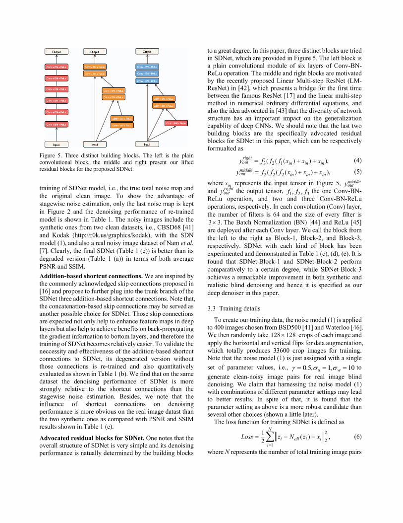
Figure 5. Three distinct building blocks. The left is the plain convolutional block, the middle and right present our lifted residual blocks for the proposed SDNet.

training of SDNet model, i.e., the true total noise map and

the original clean image. To show the advantage of

stagewise noise estimation, only the last noise map is kept

in Figure 2 and the denoising performance of re-trained

model is shown in Table 1. The noisy images include the

synthetic ones from two clean datasets, i.e., CBSD68 [41]

and Kodak (http://r0k.us/graphics/kodak), with the SDN

model (1), and also a real noisy image dataset of Nam et al.

[7]. Clearly, the final SDNet (Table 1 (e)) is better than its

degraded version (Table 1 (a)) in terms of both average

PSNR and SSIM.

Addition-based shortcut connections. We are inspired by

the commonly acknowledged skip connections proposed in

[16] and propose to further plug into the trunk branch of the

SDNet three addition-based shortcut connections. Note that,

the concatenation-based skip connections may be served as

another possible choice for SDNet. Those skip connections

are expected not only help to enhance feature maps in deep

layers but also help to achieve benefits on back-propogating

the gradient information to bottom layers, and therefore the

training of SDNet becomes relatively easier. To validate the neccessity and effectiveness of the addition-based shortcut

connections to SDNet, its degenerated version without

those connections is re-trained and also quantitatively

evaluated as shown in Table 1 (b). We find that on the same

dataset the denoising performance of SDNet is more

strongly relative to the shortcut connections than the

stagewise noise estimation. Besides, we note that the

influence of shortcut connections on denoising

performance is more obvious on the real image datast than

the two synthetic ones as compared with PSNR and SSIM

results shown in Table 1 (e).

Advocated residual blocks for SDNet. One notes that the overall structure of SDNet is very simple and its denoising

performance is natually determined by the building blocks

to a great degree. In this paper, three distinct blocks are tried

in SDNet, which are provided in Figure 5. The left block is

a plain convolutional module of six layers of Conv-BN-

ReLu operation. The middle and right blocks are motivated

by the recently proposed Linear Multi-step ResNet (LM-ResNet) in [42], which presents a bridge for the first time

between the famous ResNet [17] and the linear multi-step

method in numerical ordinary differential equations, and

also the idea advocated in [43] that the diversity of network

structure has an important impact on the generalization

capablity of deep CNNs. We should note that the last two

building blocks are the specifically advocated residual

blocks for SDNet in this paper, which can be respectively

formualted as

(4)

(5)

where represents the input tensor in Figure 5,

and the output tensor, the one Conv-BN-

ReLu operation, and two and three Conv-BN-ReLu

operations, respectively. In each convolution (Conv) layer,

the number of filters is 64 and the size of every filter is

The Batch Normalization (BN) [44] and ReLu [45]

are deployed after each Conv layer. We call the block from

the left to the right as Block-1, Block-2, and Block-3,

respectively. SDNet with each kind of block has been

experimented and demonstrated in Table 1 (c), (d), (e). It is

found that SDNet-Block-1 and SDNet-Block-2 perform

comparatively to a certain degree, while SDNet-Block-3

achieves a remarkable improvement in both synthetic and

realistic blind denoising and hence it is specified as our

deep denoiser in this paper.

3.3 Training details

To create our training data, the noise model (1) is applied

to 400 images chosen from BSD500 [41] and Waterloo [46].

We then randomly take crops of each image and

apply the horizontal and vertical flips for data augmentation,

which totally produces 33600 crop images for training.

Note that the noise model (1) is just assigned with a single

set of parameter values, i.e., to

generate clean-noisy image pairs for real image blind

denoising. We claim that harnessing the noise model (1)

with combinations of different parameter settings may lead

to better results. In spite of that, it is found that the

parameter setting as above is a more robust candidate than

several other choices (shown a little later).

The loss function for training SDNet is defined as

(6)

where N represents the number of total training image pairs

3 2 1( ( ( ) ) ),rightout in in inx x xy f f f + +=

2 2 2( ( ( ) ) ),middleout in in inx x xy f f f + +=

inx

middleouty

rightouty 1 2 3, ,f f f

3 3.×

128 128×

,0.5 1, 10u w

γ σ σ= = =

2

21

1

2( ) ,all

N

i i i

i

Loss z N z x

=

= − −∑

CBM3D WNNM Ours CBM3D WNNM Ours CBM3D WNNM Ours CBM3D WNNM Ours

CBSD68 28.19 35.64 37.54 28.16 33.31 34.59 28.19 32.54 34.53 28.15 31.69 34.34

Kodak 29.74 36.70 37.71 29.68 34.49 34.98 29.74 33.74 34.92 29.68 32.82 35.15

Average 28.96 36.17 37.63 28.91 33.90 34.79 28.96 33.14 34.73 28.91 32.26 34.75

Table 2. Denoising performance on the synthetic noisy images generated by the signal dependent noise model with different settings of

parameter values. State-of-the-art denoising methods CBM3D [5] and WNNM [6] are compared with SDNet. The bold indicates the best.

Camera Settings CBM3D [5] DnCNN [2] NC [48] WNNM [6]

MCWNNM [33]

SDNet Camera ISO Image #

Canon 5D Mark III 3200

1 38.25 37.26 38.75 39.68 39.89 39.83

2 35.85 34.13 35.55 35.75 37.03 37.25

3 34.12 34.09 35.54 34.67 35.66 36.79

Nikon D600 3200

1 33.10 33.62 35.57 33.60 34.83 35.50

2 35.57 34.48 36.79 36.32 36.50 37.24

3 40.77 35.41 39.26 39.95 38.87 41.18

Nikon D800 1600

1 36.83 35.79 38.03 36.63 38.46 38.77

2 40.19 36.08 39.02 40.28 39.78 40.87

3 37.64 35.48 38.21 37.56 39.01 38.86

Nikon D800 3200

1 39.72 34.08 38.03 38.68 37.76 39.94

2 36.74 33.70 35.69 36.42 36.53 36.78

3 40.96 33.31 36.76 39.86 37.76 39.78

Nikon D800 6400

1 34.63 29.83 33.52 34.43 32.91 33.34

2 33.95 30.55 32.79 32.81 32.67 33.29

3 33.61 30.09 32.80 32.72 33.17 33.22

Average 36.73 33.86 36.42 36.62 36.66 37.51

Table 3. Performance comparison of different blind denoising methods on the real image dataset of Nam et al. [7], including CBM3D [5], DnCNN [2], NC [48], WNNM [6], MCWNNM [33], and our SDNet. The bold indicates the best.

and describes the total noise map as

explained in subsection 3.2. The minimization method is

the Adam algorithm [47] with the learning rate degrading

from 10-4 to 10-6, and 10-6. The

size of mini-batch is set as 16 and the model is trained 50

epochs. It takes approximately 10 hours to train our SDNet

model on a Nvidia GeForce CTX 1080 Ti GPU.

4. Experiments

4.1 Synthetic denoising results

To validate denoising performance of SDNet on

synthetic noisy images, four groups of clean-noisy pairs are

prepared in the same manner as subsection 3.3 except that the signal dependent noise model (1) is assigned with different settings of parameter values as listed in Table 2. Two state-of-the-art classical algorithms CBM3D [5] and WNNM [6] are of our

particular interest for comparison with the proposd SDNet.

Denoising experiments are performed on the noisy images synthesized from two clean datasets, i.e., CBSD68 [41] (68

images) and Kodak (24 images). We see that the proposed SDNet

has achieved universal better performance than both

CBM3D and WNNM in four groups of synthetic datasets.

In spite of that, the SDNet with is

to be employed to process the two real image datasets in

this paper because of its more adaptiveness to the

corresponding blind denoising tasks.

4.2 Realistic denoising results

This section demonstrates denoising performance of the

SDNet algorithm on two realistic noisy image datasets

along with comparison to state-of-the-art real denoising

methods including MCWNNM [33] and NC [48], and three

leading AWGN denoising methods including CBM3D [5],

WNNM [6] and DnCNN [2]. We note that, there are much

0.5, 0.5, 5u w

γ σ σ= = = 0.5, 0.5, 10u w

γ σ σ= = = 0.5, 1, 5u w

γ σ σ= = = 0.5, 1, 10u w

γ σ σ= = =

1,{( )}Nii ixz = ( )all iN z

1 0.9,β = 2 ,0.999β = ε =

,0.5 1, 10u w

γ σ σ= = =

CBM3D [5] DnCNN [2] NC [48] WNNM [6] MCWNNM [33] Our SDNet

38.25 dB 37.26 dB 38.75 dB 39.11 dB 39.68 dB 39.83 dB

37.64 dB 35.48 dB 38.21 dB 37.05 dB 39.01 dB 38.86 dB

39.72 dB 34.08 dB 38.03 dB 38.66 dB 38.68 dB 39.94 dB

36.83 dB 35.79 dB 38.03 dB 36.63 dB 38.46 dB 38.77 dB

34.12 dB 34.09 dB 35.54 dB 34.67 dB 35.66 dB 36.79dB

Figure 6. Denoising results of several images from the dataset in Nam et al. [7] corresponding to each denoising method.

less real image denoisers than the AWGN ones in the

literature and their running codes are generally either not

available or hard to be employed except the noise clinic

(NC) [48] and multi- channel WNNM (MCWNNM) [33].

The first group of experiments are performed on the real

dataset of Nam et al. [7] totally consisting of 11 static

scenes, 500 JPEG images per scene which are averaged as

the mean image to be the corresponding ground truth. It is

noted that the noise of in-camera imaging processing is also taken into consideration in this dataset. Moreover, a new

cross-channel noise model is proposed Nam et al. [7]. The

original images of the dataset are captured by Nikon D800,

Nikon D600 and Canon 5D Mark III with different ISO

values, most of which are with the size and

are then cropped into the size The PSRN scores

of denoised results using each method are provided in Table

2. Not surprisingly, we find that DnCNN [2] achieves the

worst performance in this scenario, and it is so inferior to

the other compared methods that its average PSNR is less than others at least 2.5dB. It is interesting to find that the

two AWGN denoisers CBM3D [5] and WNNM [6] have

7630 4912×

512 512.×

CBM3D [5] DnCNN [2] NC [48] WNNM [6] MCWNNM [33] Our SDNet

34.63/0.9803 32.82/0.8769 33.90/0.9529 34.38/0.9708 34.48/0.9668 35.00/0.9863

37.07/0.9727 36.69/0.9420 36.64/0.9687 37.24/0.9597 37.45/0.9673 37.61/0.9820

Figure 7: Denoising results on two real noisy images of the PloyU dataset [40] for visual perception.

Methods CBM3D [5] NC [48] DnCNN [2] WNNM [6] MCWNNM [33] SDNet

PSNR 38.11 36.92 36.08 37.30 38.25 38.20

SSIM 0.9832 0.9449 0.9161 0.9610 0.9665 0.9846

Table 4: Performance comparison of different blind denoising methods on the PloyU real image dataset [40] (100 images) including CBM3D [5], DnCNN [2], NC [48], WNNM [6], MCWNNM [33], and our SDNet. The bold indicates the best.

been very competitive to the two real denoisers NC [48] and

MCWNNM [33] to a great degree. In this experiment,

SDNet is demonstrated rather qualified for denoising of real

photographs in Nam et al. [7] inspite of its blindness to the

camera image signal processing pipeline. In Figure 4 the

noisy images are provided and in Figure 6 some of denoising results by each approach are shown for visual

perception. We also perform blind denoising on another

real dataset, i.e., PloyU [40] (100 real noisy photographs).

Table 3 provides the PSNR and SSIM scores for each

denoising method on this dataset. In this experiment, it is

found that SDNet achieves a competitive performance to

the AWGN method CBM3D [5] and real denoiser

MCWNNM [33], and a superior performance than NC [48],

DnCNN [2], as well as WNNM [6]. Denoising results are

provided in Figure 7 for visual comparison corresponding

to each method on two real noisy photographs of PolyU.

5. Conclusion

This paper proposes a simple yet robust deep convolution

approach to blind denoising of real camera photographs, i.e.,

SDNet. It is formulated as a fully end-to-end convolutional

residual neural model for stagewise denoising, strengthened

by lifted residual modules and the shortcut connections.The

model is trained without use of any hand-crafted priors or

additional real noisy photographs. Experimental results on both simulated and real noisy images show that the new

blind denoiser achieves competitive or better performance

than state-of-the-art classical and deep denoising

algorithms in terms of both quantitative and qualitative

assessment.

Acknowledgment

The study is supported in part by the Natural Science

Foundation (NSF) of China (61771250, 61602257,

61572503, 61872424, 61972213, 6193000388), and the

NSF of Jiangsu Province (BK20160904).

References

[1] Y. Chen, T. Pock. Trainable nonlinear reaction diffusion: A flexible framework for fast and effective image restoration. IEEE Trans. PAMI, 39:1256–1272, 2017. [2] K. Zhang, W. Zuo, Y. Chen, D. Meng, and L. Zhang. Beyond a gaussian denoiser: Residual learning of deep cnn for image denoising. TIP, 26: 3142–3155, 2017. [3] T. Plotz and S. Roth. Benchmarking denoising algorithms with

real photographs. In CVPR, 2017. [4] K. Dabov, A. Foi, V. Katkovnik, et al. Image denoising by sparse 3-D transform-domain collaborative filtering. TIP, 16(8): 2080-2095, 2007. [5] K. Dabov, A. Foi, V. Katkovnik, and K. Egiazarian. Color image denoising via sparse 3D collaborative filtering with grouping constraint in luminance-chrominance space. In ICIP, 2007.

[6] S. Gu, L. Zhang, W. Zuo, and X. Feng. Weighted nuclear norm minimization with application to image denoising. In CVPR, 2014. [7] S. Nam, Y. Hwang, Y. Matsushita, S.J. Kim. A holistic approach to cross-channel image noise modeling and its application to image denoising. In CVPR, 2016.

[8] J. Mairal, F. Bach, J. Ponce, G. Sapiro, and A. Zisserman. Non-local sparse models for image restoration. In ICCV, 2009. [9] S. Roth and M. J. Black. Fields of experts. International Journal of Computer Vision, 82(2):205–229, 2009. [10] G. Yu, G. Sapiro, and S. Mallat. Solving inverse problems

with piecewise linear estimators: From Gaussian mixture models to structured sparsity. TIP, 21(5): 2481–2499, 2012. [11] W. Dong, G. Shi, Y. Ma, and X. Li. Image restoration via simultaneous sparse coding: Where structured sparsity meets gaussian scale mixture. IJCV, 114(2): 217–232, 2015. [12] M. Lebrun, M. Colom, and J.-M. Morel. Multiscale image blind denoising. TIP, 24(10): 3149– 3161, 2015. [13] J. Xu, L. Zhang, D. Zhang, and X. Feng. Multi-channel

weighted nuclear norm minimization for real color image denoising. In ICCV, 2017. [14] M. Elad and M. Aharon. Image denoising via sparse and redundant representations over learned dictionaries. TIP, 15(12): 3736-3745, 2006. [15] T. Remez, O. Litany, R. Giryes, A.M. Bronstein. Deep convolutional denoising of low-light images. arXiv:1701.01687, 2017.

[16] X.-J. Mao, C. Shen, Y.-B. Yang. Image restoration using very deep convolutional encoder-decoder networks with symmetric skip connections. In NIPS, 2016. [17] K. He, X. Zhang, S. Ren, J. Sun. Deep residual learning for image recognition. In CVPR, 2016. [18] X. Liu, M. Tanaka, M. Okutomi. Practical signal-dependent noise parameter estimation from a single noisy image. TIP, 23: 4361–4371, 2014.

[19] T. Chan, J. Shen. Image Processing and Analysis: Variational, PDE, Wavelet, and Stochastic Methods. SIAM, 2005. [20] A. Lanza A, S. Morigi, F. Sgallari, et al. Variational image denoising based on autocorrelation whiteness. SIAM Journal on Imaging Sciences, 6(4):1931-1955, 2013. [21] A. Buades, B. Coll, J.M. Morel. Self-Similarity-based Image denoising. Communications of the ACM, 54(5): 109-117, 2011. [22] M. Aharon, M. Elad, A. Bruckstein. K-SVD: An algorithm for designing overcomplete dictionaries for sparse representation.

Trans. Sig. Proc., 2006. [23] S. Roth and M. J. Black. Fields of experts. IJCV, 2009 [24] K. Zhang, W. Zuo, and L. Zhang. Ffdnet: Toward a fast and flexible solution for cnn based image denoising. CoRR, abs/1710.04026, 2017. [25] Y. Tai, J. Yang, X. Liu, and C. Xu. Memnet: A persistent memory network for image restoration. In ICCV, 2017. [26] D. Yang, J. Sun. Bm3d-net: A convolutional neural network

for transform-domain collaborative filtering. IEEE Signal Processing Letters, 25:55–59, 2018. [27] P. Liu, H. Zhang, K. Zhang, L. Lin, and W. Zuo. Multi-level wavelet-cnn for image restoration. CoRR, abs/1805.07071, 2018. [28] A. Foi, M. Trimeche, V. Katkovnik, and K. Egiazarian. Practical poissonian-gaussian noise modeling and fitting for single-image raw-data. IEEE Trans. Image Processing, 2008. [29] S.W. Hasinoff, F. Durand, W.T. Freeman. Noise optimal

capture for high dynamic range photography. In CVPR, 2010. [30] C. Liu, R. Szeliski, S.B. Kang, C.L. Zitnick, W.T. Freeman. Automatic estimation and removal of noise from a single image. IEEE Trans. PAMI, 2008. [31] M. Lebrun, A. Buades, J.M. Morel. A nonlocal bayesian image denoising algorithm. SIAM Journal on Imaging Sciences, 2013.

[32] F. Zhu, G. Chen, P.A. Heng. From noise modeling to blind image denoising. In CVPR, 2016. [33] J. Xu, L. Zhang, D. Zhang, and X. Feng. Multi-channel weighted nuclear norm minimization for real color image denoising. In ICCV, 2017.

[34] S. Guo, Z. Yan, K. Zhang, W. Zuo, and L. Zhang. Toward convolutional blind denoising of real photographs. In CVPR, 2019. [35] J. Chen, J. Chen, H. Chao, M. Yang. Image blind denoising with generative adversarial network based noise modeling. In CVPR, 2018. [36] J. Lehtinen, J. Munkberg, J. Hasselgren, S. Laine, T. Karras, M. Aittala, and T. Aila. Noise2noise: Learning image restoration without clean data. arXiv:1803.04189, 2018.

[37] S. Soltanayev and S. Y. Chun. Training deep learning based denoisers without ground truth data. In NIPS, 2018. [38] J. Anaya, A. Barbu. RENOIR-A benchmark dataset for real noise reduction evaluation. Computer Science, 51: 144-154, 2014. [39] T. Plotz, S. Roth. Benchmarking denoising algorithms with real photographs. In CVPR, 2017. [40] J. Xu, H. Li, Z. Liang, D. Zhang, L. Zhang. Real-world noisy image denoising: A new benchmark. CoRR, abs/1804.02603,

2018. [41] D. Martin, C. Fowlkes, D. Tal, and J. Malik. A database of human segmented natural images and its application to evaluating segmentation algorithms and measuring ecological statistics. In ICCV, 2001. [42] Y. Lu, A. Zhong, Q. Li, B. Dong. Beyond finite layer neural network: Bridging deep architects and numerical differential equations. In ICML, 2018.

[43] X. Zhang, Z. Li, C. Loy, and D. Lin. Polynet: A pursuit of structural diversity in very deep networks. In CVPR, 2017. [44] S. Ioffe and C. Szegedy. Batch normalization: Accelerating deep network training by reducing internal covariate shift. In ICML, 2015. [45] V. Nair and G.E. Hinton. Rectified linear units improve restricted boltzmann machines. In ICML, 2010. [46] K. Ma, Z. Duanmu, Q. Wu, Z. Wang, H. Yong, H. Li, and L. Zhang. Waterloo exploration database: New challenges for image

quality assessment models. TIP, 26:1004–1016, 2016. [47] D. Kingma and J. Ba. Adam: A method for stochastic optimization. In ICLR, 2015. [48] M. Lebrun, M. Colom, and J.-M. Morel. Multiscale image blind denoising. TIP, 24(10):3149– 3161, 2015.