Embed Size (px)
Citation preview
1
A Short course of LS-DYNA/MPP®
Jason Wang
Jan 26, 2010
Contents
� IntroductionDevelopment History
What drives the MPP development?
Implementation of SMP and MPP
Implementation in production
Numerical variations
Performance
� Scalability of LS-DYNA/MPP“Scalability”Effects of InterconnectsEffect of CompilerDistribution of the CPU timeEffect of DecompositionSummary
� Special DecompositionDecomposition Methods in LS-DYNA®
General pfile and *CONTROL_MPP commands
Load Balancing
Case Studies
Bumper Impact
Side Impact
ODB
Metal Forming
ALE Airbag Simulation
Special MPP features
General Guidelines
� MPP ContactMPP Contact Algorithms
MPP Contact Options
Groupable Contact
*CONTACT_FORCE_TRANSDUCER
Contact General Guidelines
2
Contents
� General GuidelinesNumerical Consistency
Debugging
Cluster Tuning
Pre-decomposition
Restart
� Current Benchmark tests3cars
Neon refined
Car2car
� Recent DevelopmentsCurrent Development
Scalability to Large Number of Processors
Introduction
3
• Development History
• What drives the MPP development?
• Implementation in production
• Implementation of SMP and MPP
• Numerical variations
• Performance
Introduction
� Public domain DYNA3D, Dr. John O. Hallquist/Lawrence Livermore National Laboratory, 1976
� Weapon simulations
� LSTC and LS-DYNA3D® founded by Dr. J. O. Hallquist in 1988
� Recognized market for commercial applications
� In the 1990’s …
� LS-DYNA2D and LS-DYNA3D® combined (LS-DYNA)
� Implicit capability (LS-NIKE3D) introduced to LS-DYNA®
� Thermal capability (TOPAZ) introduced to LS-DYNA®
� Introduced MPP capability
� Eulerian/ALE element formulations and Euler/Lagrange coupling introduced
� LS-POST, LS-OPT® introduced
Development History
4
� Since 2000,
� Expanded MPP capability
� Meshless methods introduced
� LS-POST expanded to include preprocessing (LS-PrePost®)
� Worldwide distribution: US, UK, Nordic countries, France, Germany, Italy, Netherlands, Japan, Korea, China,Taiwan, India, Brazil; also through ANSYS and MSC.
� 60+ full-time employees + numerous consultants
� Products:
� LS-DYNA®
� LS-PrePost®
� LS-OPT®
� FE Models: Dummies, barriers, head forms
� USA (Underwater Shock Analysis)
Development History
• Automotive – Crash and safety– Durability– NVH
• Aerospace– Bird strike– Containment
– Crash• Manufacturing
– Stamping– Forging
• Structural– Earthquake safety– Concrete structures
• Electronics– Drop analysis– Package design– Thermal
• Defense
– Weapon design– Blast response– Penetration– Underwater shock analysis
• Also, applications in biomedical, sports, consumer products, etc.
Development History
5
9
• Combine the multi-physics capabilities • Explicit/Implicit solver
• ALE, SPH, EFG• Heat Transfer• Airbag particle method• Acoustics (USA)• Interfaces for users, i.e., elements, materials, loads
• Electromagnetic (version 981)• Incompressible fluids (version 981)• CESE compressible fluid solver (version 981)
• into one scalable code for solving highly nonlinear transient problems to enable the solution of coupled multi-physics and multi-stage problems.
Development History
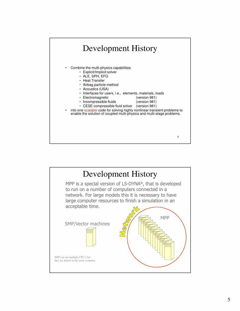
Development HistoryMPP is a special version of LSMPP is a special version of LS--DYNADYNA®®, that is developed , that is developed to run on a number of computers connected in a to run on a number of computers connected in a network. For large models this it is necessary to have network. For large models this it is necessary to have large computer resources to finish a simulation in an large computer resources to finish a simulation in an acceptable time.acceptable time.
SMP/Vector machines
MPP
SMP can run multiple CPU’s but
they are placed in the same computer
6
• SMP (Shared Memory Parallel)
– Start and base from serial code
– Using OpenMP directives to split the tasks
– Only run on SMP (single image) computers
– Scalable up to ~8 CPUs
• MPP (Message Passing Parallel)
– Using the domain decomposition method
– Using MPI for communications between sub-domains
– Work on both SMP machines and clusters
– Scalable >> 8 CPUS
– Dramatically reduced elapsed time and the simulation cost
Development History
• MPP-DYNA was initiated in 1993 (version 930)
• Nearly fully supported contact algorithms (1996)
• P-file, composition and analyze in one run (1996)
• CONSTRAINED_options (1996)
• Limited ALE capabilities (1998)
• SPH (2002)
• EFG (971)
• Thermal (971)
• Constantly development, recently some feature first in MPP, before they appears in MPP!
Development History
Many of the features were implemented as customers Many of the features were implemented as customers required it. This means that features were not required it. This means that features were not implemented in option blocks.implemented in option blocks.
7
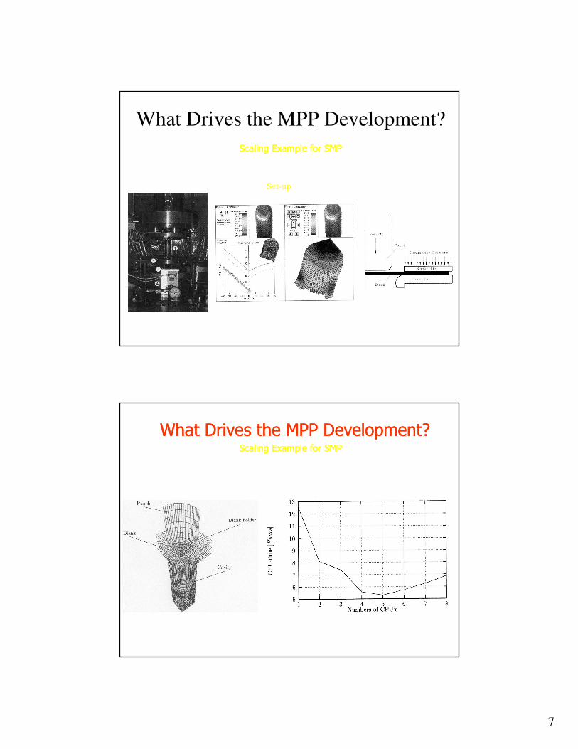
• Scaling for SMP simulating Conventional
Cylindrical Deep Drawing [Moshfegh et al,
1998]
Scaling Example for SMPScaling Example for SMP
Set-up
What Drives the MPP Development?
• The turn around for this model is found to
be 5 CPU’s.
Scaling Example for SMPScaling Example for SMP
What Drives the MPP Development?What Drives the MPP Development?
8
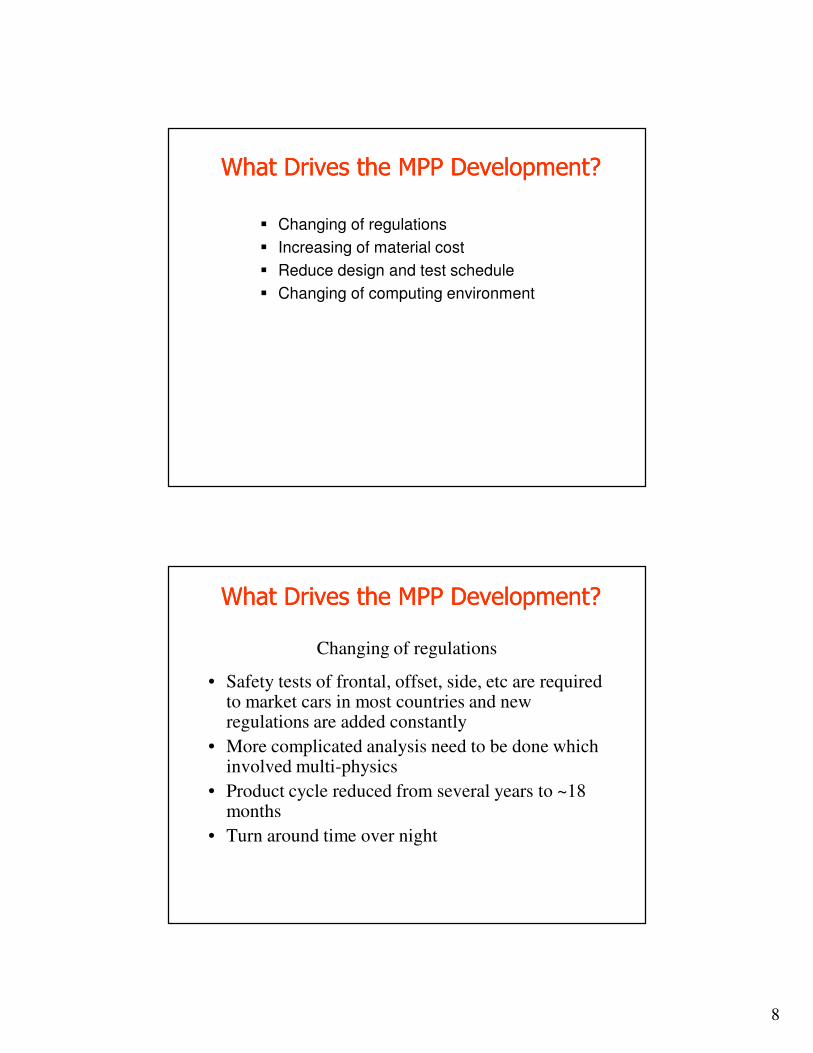
� Changing of regulations
� Increasing of material cost
� Reduce design and test schedule
� Changing of computing environment
What Drives the MPP Development?What Drives the MPP Development?
Changing of regulations
• Safety tests of frontal, offset, side, etc are required to market cars in most countries and new regulations are added constantly
• More complicated analysis need to be done which involved multi-physics
• Product cycle reduced from several years to ~18 months
• Turn around time over night
What Drives the MPP Development?What Drives the MPP Development?
9
• Smaller and smaller element size
• More expansive element formulation
• Non-local failure (reduce analysis noise)
• Complicated spotweld capabilities (cluster of solids)
• More sophisticated material models
Longer simulation time
Changing of modeling
• Multi-physics: ALE + FSI - airbag, fuel tank
• Multi-physics: EM + metal forming
• Fine meshed barrier
• Bio-dummy
• Crash model with stamped parts
Much longer simulation time
Changing of modeling to Include
Multi-Physics and Multi-Stages
10
Cost reduction
• Produce more durable end products
• Save raw material in production line– few grams per product but save millions dollars in
production
• Product cycle reduced from 1 year to 3 months
• Turn around time in few hours
What Drives the MPP Development?What Drives the MPP Development?
Reduce design to test cycle
What Drives the MPP Development?What Drives the MPP Development?
11
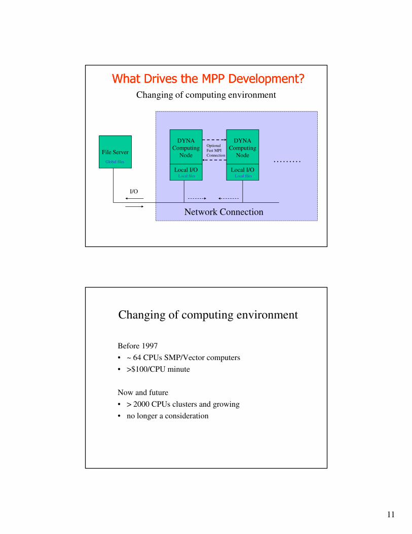
Changing of computing environment
File Server
………
Network Connection
DYNA
Computing
Node
Local I/O
DYNA
Computing
Node
Local I/O
I/O
Optional
Fast MPI
Connection
Local files
Global files
Local files
What Drives the MPP Development?What Drives the MPP Development?
Changing of computing environment
Before 1997
• ~ 64 CPUs SMP/Vector computers
• >$100/CPU minute
Now and future
• > 2000 CPUs clusters and growing
• no longer a consideration
12
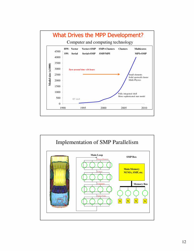
0
500
1000
1500
2000
2500
3000
3500
4000
4500
1990 1995 2000 2005 2010
Mod
el s
ize
(x1
00
0)
Turn around time <16 hours
BT shell
Fully integrated shell
More sophisticated mat model
HW: Vector Vector+SMP SMP+Clusters Clusters Multicores
SW: Serial Serial+SMP SMP/MPI MPI+SMP
Small elements
Solid spotweld cluster
Multi-Physics
Computer and computing technology
What Drives the MPP Development?What Drives the MPP Development?
Implementation of SMP Parallelism
Main Loop
$ $ $ $
Main Memory
NUMA, SMP, etc.
Memory Bus
SMP BoxProcess Elements
Contact
Constraints
Update Nodes
13
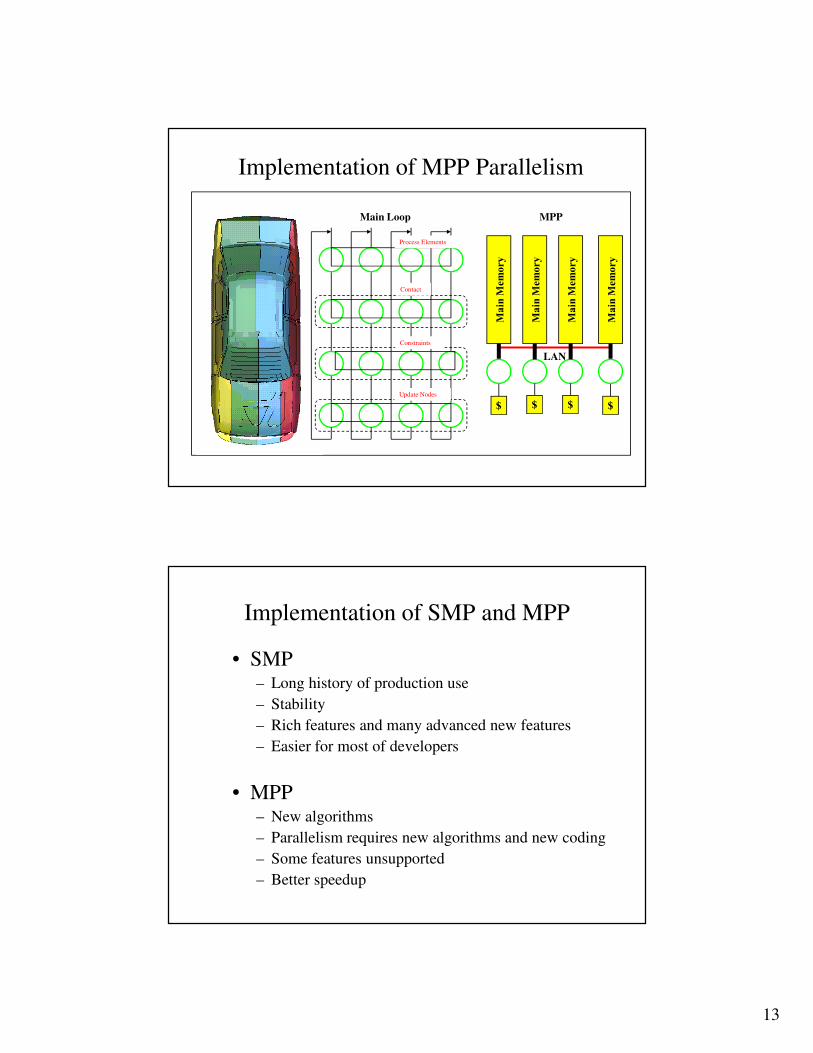
Implementation of MPP Parallelism
Main Loop
$ $ $ $
MPP
LAN
Process Elements
Contact
Constraints
Update Nodes
Implementation of SMP and MPP
• SMP– Long history of production use
– Stability
– Rich features and many advanced new features
– Easier for most of developers
• MPP – New algorithms
– Parallelism requires new algorithms and new coding
– Some features unsupported
– Better speedup
14
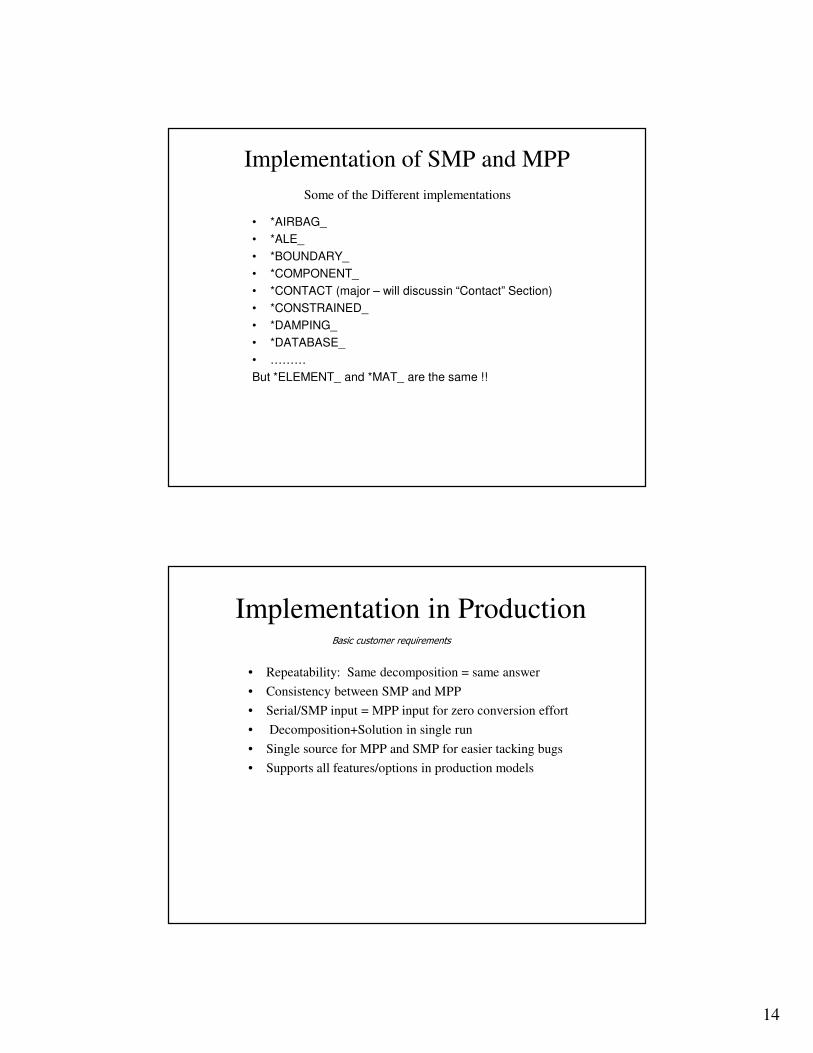
Implementation of SMP and MPP
• *AIRBAG_
• *ALE_
• *BOUNDARY_
• *COMPONENT_
• *CONTACT (major – will discussin “Contact” Section)
• *CONSTRAINED_
• *DAMPING_
• *DATABASE_
• ………
But *ELEMENT_ and *MAT_ are the same !!
Some of the Different implementations
Implementation in Production
• Repeatability: Same decomposition = same answer
• Consistency between SMP and MPP
• Serial/SMP input = MPP input for zero conversion effort
• Decomposition+Solution in single run
• Single source for MPP and SMP for easier tacking bugs
• Supports all features/options in production models
Basic customer requirements
15
Implementation in Production• MPP project starts from 1993
• Chrysler 1998
– Phase I (Q3/98) – 30 6-month old models
• Check for missing features
• SMP/MPP performance, results comparison
• Open 2 12-processor queue
– Phase II (Q1/99) – 20 production models
• SMP/MPP performance, results comparison
• Open 8 12-processor queues
– Phase III (Q2/99) - 5 models for QA
• SMP/MPP performance, results comparison
• Madymo coupling
• Open 16 12-processor queues + Open several
24-processor queues for high priority jobs
Fully production in 1999 and most jobs finished overnight
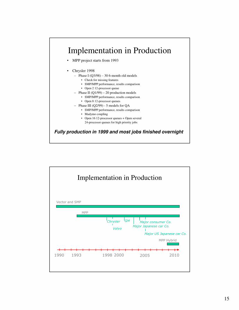
Vector and SMP
Introduction
1990 1993 1998 2010
MPP
MPP Hybrid
2000 2005
Chrysler
Volvo
GM
Major Japanese car Co.
Major consumer Co.
Implementation in Production
Major US Japanese car Co.
16
Implementation in Production
• ~ 64 CPUs SMP/Vector DYNA Nodes at 1996
800 CPUs clusters and growing
• >$100/minute at 1996 less $1/minute
• 3 days/job (100K elements) overnight turn
around time (1 million elements+more)
• 2009: 3 million elements – overnight!
Impact of Computing EnvironmentImpact of Computing Environment
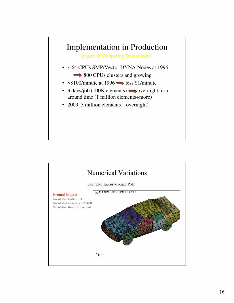
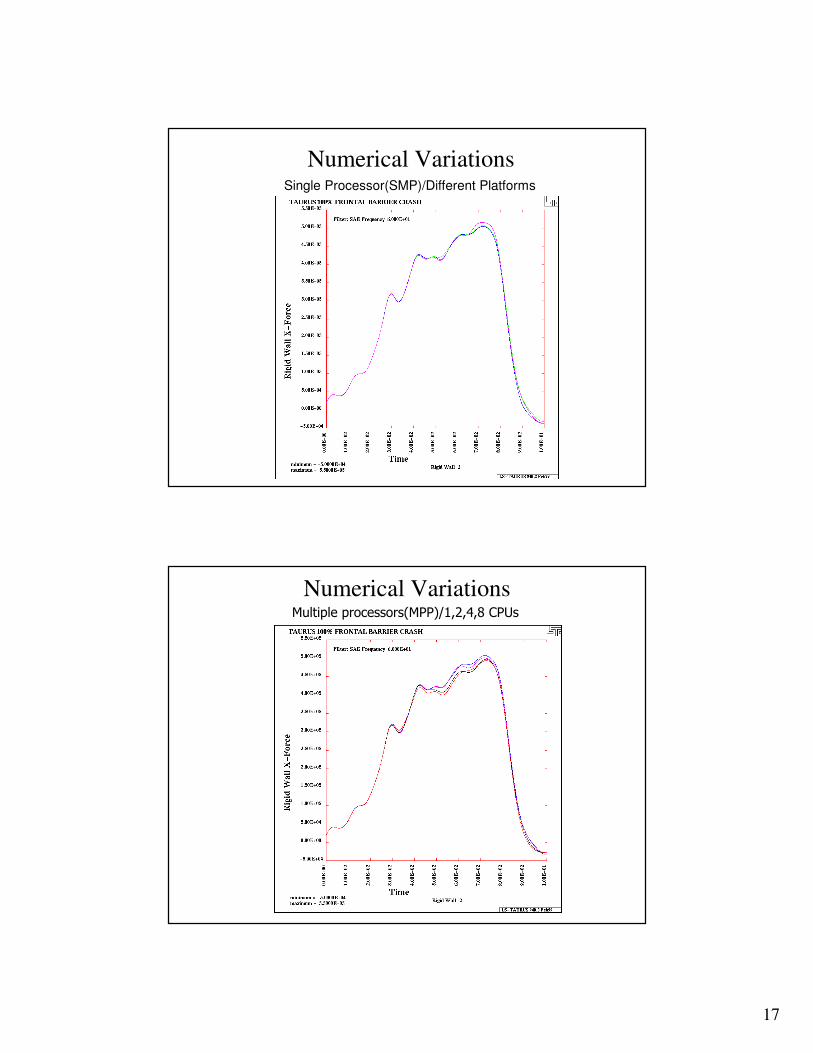
Numerical Variations
Example: Taurus to Rigid Pole
Frontal impact:No. of materials: ~130
No. of shell elements: ~28,000
Simulation time: 0.10 second
17
Numerical VariationsSingle Processor(SMP)/Different Platforms
Numerical VariationsMultiple processors(MPP)/1,2,4,8 CPUs
18
Numerical Variations
• Round off error – DP may give less error
• DP may not help, finer mesh may help
• Changing number of processors 5% (MPP), however for a good stable model the difference is small (2009)
• Look for errors in the model – different platforms handles
the division by zero differently
• Differences in MPP and SMP contact
• For SMP use consistency command (ncpu=-integer)
Performance Comparison
Example: Neon Refined Model
� Frontal crash with initial speed at 31.5 miles/hour
� Model size
� Number of nodal points: 532077
� Number of shell elements: 535K
� Simulation length: 30 ms
� Model created by National Crash Analysis Center (NCAC) at George Washington University
� One of the few publicly available models for vehicle crash analysis
� Based on 1996 Plymouth Neon
� Modified by LSTC (refined the mesh)
19
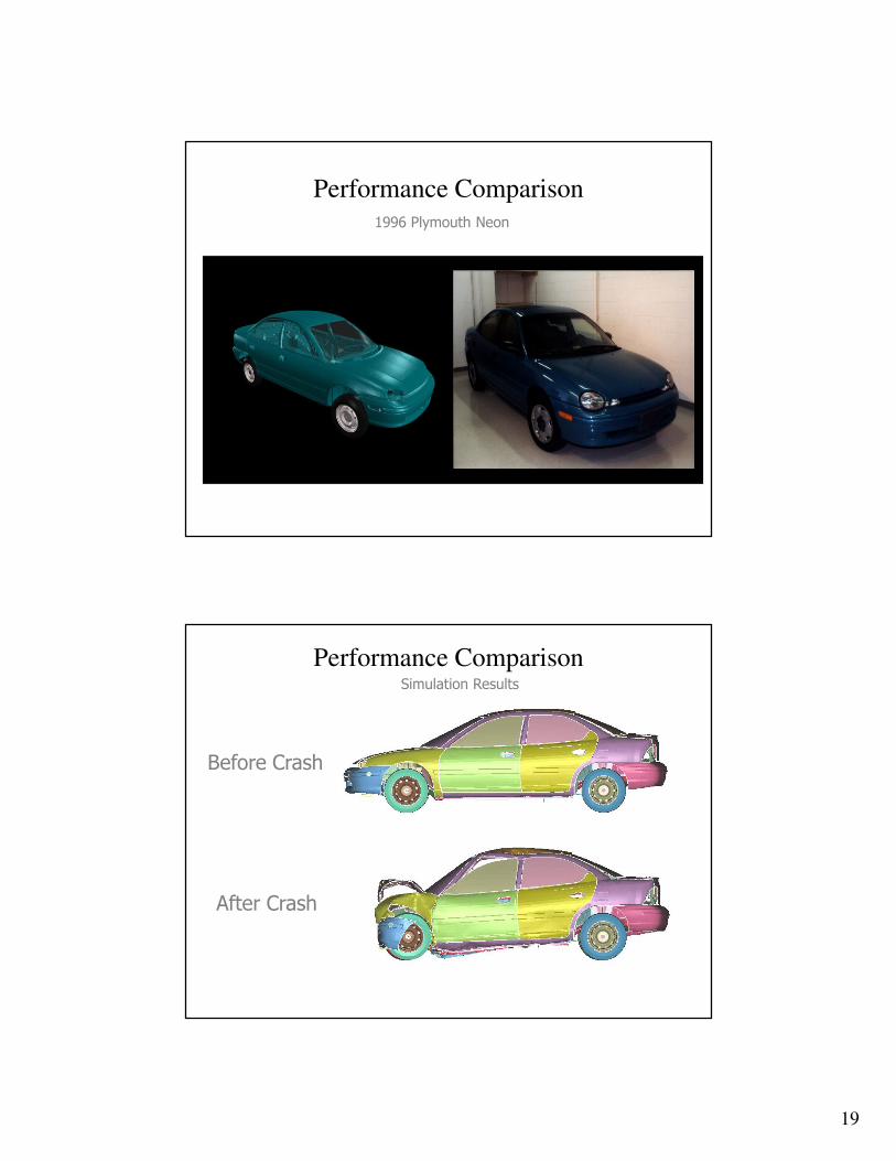
Performance Comparison1996 Plymouth Neon
Performance Comparison
After Crash
Before Crash
Simulation Results
20
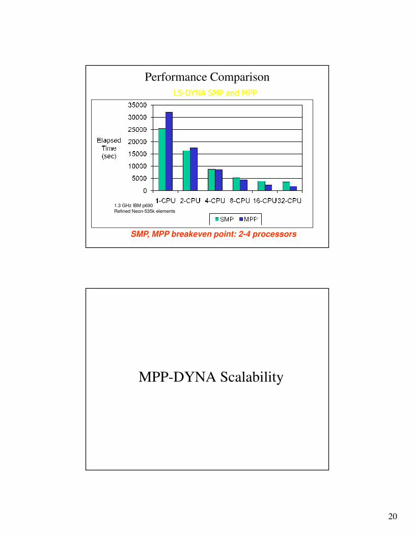
Performance Comparison
LSLS--DYNA SMP and MPPDYNA SMP and MPP
1.3 GHz IBM p690
Refined Neon-535k elements
SMP, MPP breakeven point: 2-4 processors
MPP-DYNA Scalability
21
MPP-DYNA Scalability
� “Scalability”
� Effects of Interconnects
� Effect of Compiler
� Distribution of the CPU time
� Effect of Decomposition
� Summary
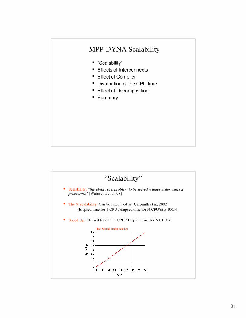
“Scalability”
� Scalability: ”the ability of a problem to be solved n times faster using n processors” [Wainscott et al, 98]
� The % scalability: Can be calculated as [Galbraith et al, 2002]:
(Elapsed time for 1 CPU / elapsed time for N CPU’s) x 100/N
� Speed Up: Elapsed time for 1 CPU / Elapsed time for N CPU’s
Ideal Scaling (linear scaling)
22
Main factors that influence scalability/performance:
� Decomposition of the model, due to load balance
(Will be discussed in “Decomposition” section)
� Single node computational performance
� Characteristics of the interconnection
Ethernet, IB, etc
NFS, local disks
� Message Passing details
� Memory/Cache System
� Model size and problem type
“Scalability”
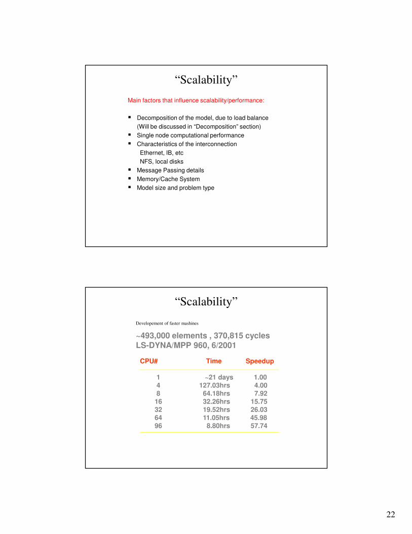
~493,000 elements , 370,815 cycles LS-DYNA/MPP 960, 6/2001
CPU# Time Speedup
1 ~21 days 1.00
4 127.03hrs 4.00
8 64.18hrs 7.92
16 32.26hrs 15.75
32 19.52hrs 26.03
64 11.05hrs 45.98
96 8.80hrs 57.74
Developement of faster mashines
“Scalability”
23
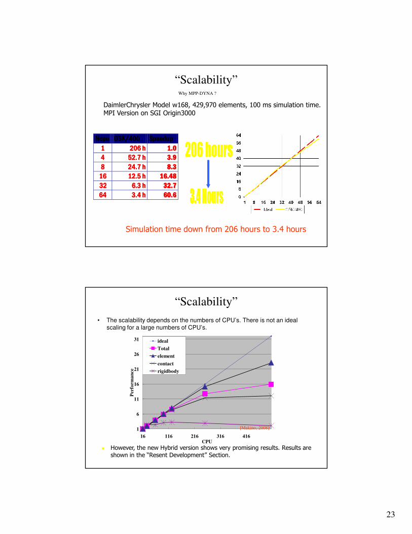
NcpuNcpuNcpuNcpu O3K/400O3K/400O3K/400O3K/400 SpeedupSpeedupSpeedupSpeedup
1111 206 h206 h206 h206 h 1.01.01.01.0
4444 52.7 h52.7 h52.7 h52.7 h 3.93.93.93.9
8888 24.7 h24.7 h24.7 h24.7 h 8888....3333
16161616 12.5 h12.5 h12.5 h12.5 h 16161616....48484848
32 32 32 32 6.3 h6.3 h6.3 h6.3 h 33332222....7777
64646464 3.4 h3.4 h3.4 h3.4 h 66660000....6666
Simulation time down from 206 hours to 3.4 hours
DaimlerChrysler Model w168, 429,970 elements, 100 ms simulation time. MPI Version on SGI Origin3000
Why MPP-DYNA ?
“Scalability”
1
6
11
16
21
26
31
16 116 216 316 416CPU
Per
form
an
ce
ideal
Total
element
contact
rigidbody
• The scalability depends on the numbers of CPU’s. There is not an ideal scaling for a large numbers of CPU’s.
� However, the new Hybrid version shows very promising results. Results are shown in the “Resent Development” Section.
[Makino, 2008]
“Scalability”
24
Effects of Interconnects
� Computation is split up into:
T_elapsed = T_computation + T_communication + T_IO
– For a cluster the communication time is the time required for messages
passing through the interconnection [Lin et al, 2000]
� Different types of interconnects
– 100 BASET (TCP/IP) (2009: less used)
– Gegi (TCP/IP) (2009: less used)
– Myrinet (MyriCom)
– InfiniBand (Popular)
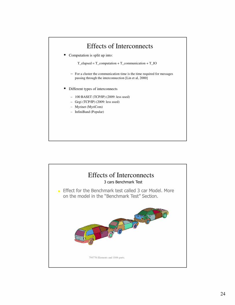
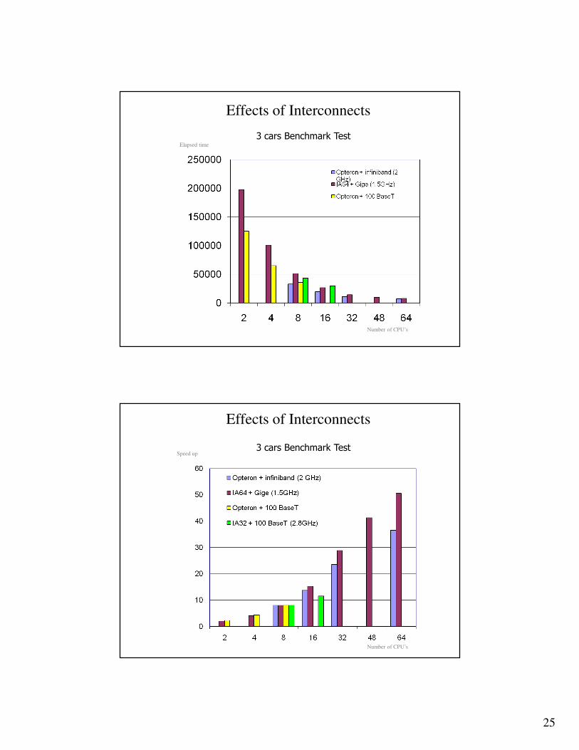
3 cars Benchmark Test
Effects of Interconnects
�� Effect for the Benchmark test called 3 car Model. More Effect for the Benchmark test called 3 car Model. More on the model in the “Benchmark Test” Section.on the model in the “Benchmark Test” Section.
794776 Elements and 1046 parts.
25
3 cars Benchmark Test
Effects of Interconnects
Elapsed time
Number of CPU’s
3 cars Benchmark Test
Effects of Interconnects
Number of CPU’s
Speed up
26
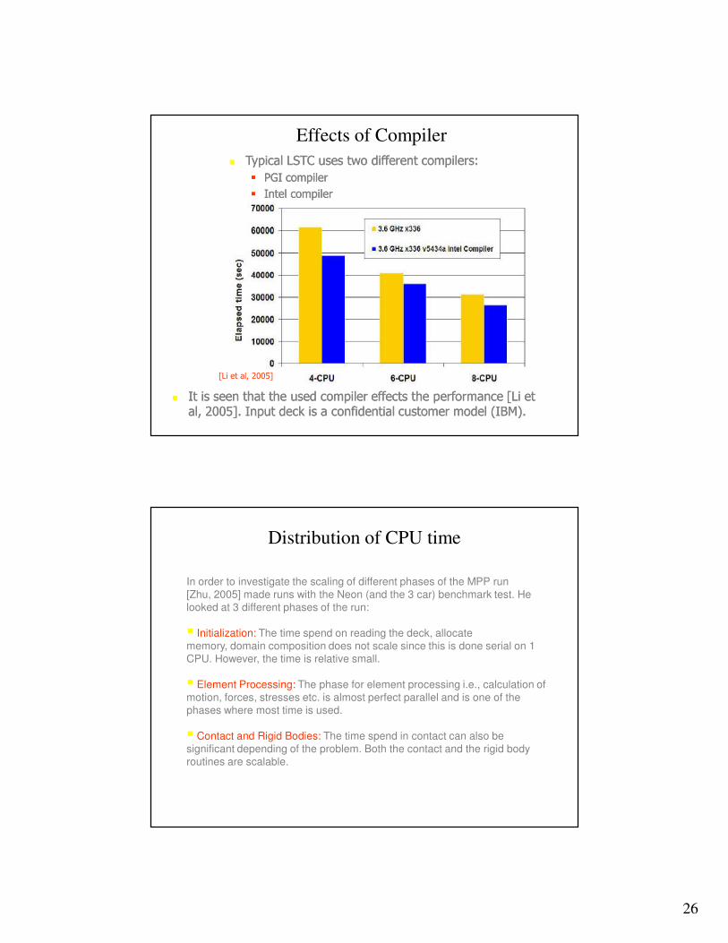
Effects of Compiler
�� Typical LSTC uses two different compilers:Typical LSTC uses two different compilers:
�� PGI compilerPGI compiler
�� Intel compilerIntel compiler
�� It is seen that the used compiler effects the performance [Li et It is seen that the used compiler effects the performance [Li et al, 2005]. Input deck is a confidential customer model (IBM).al, 2005]. Input deck is a confidential customer model (IBM).
[Li et al, 2005]
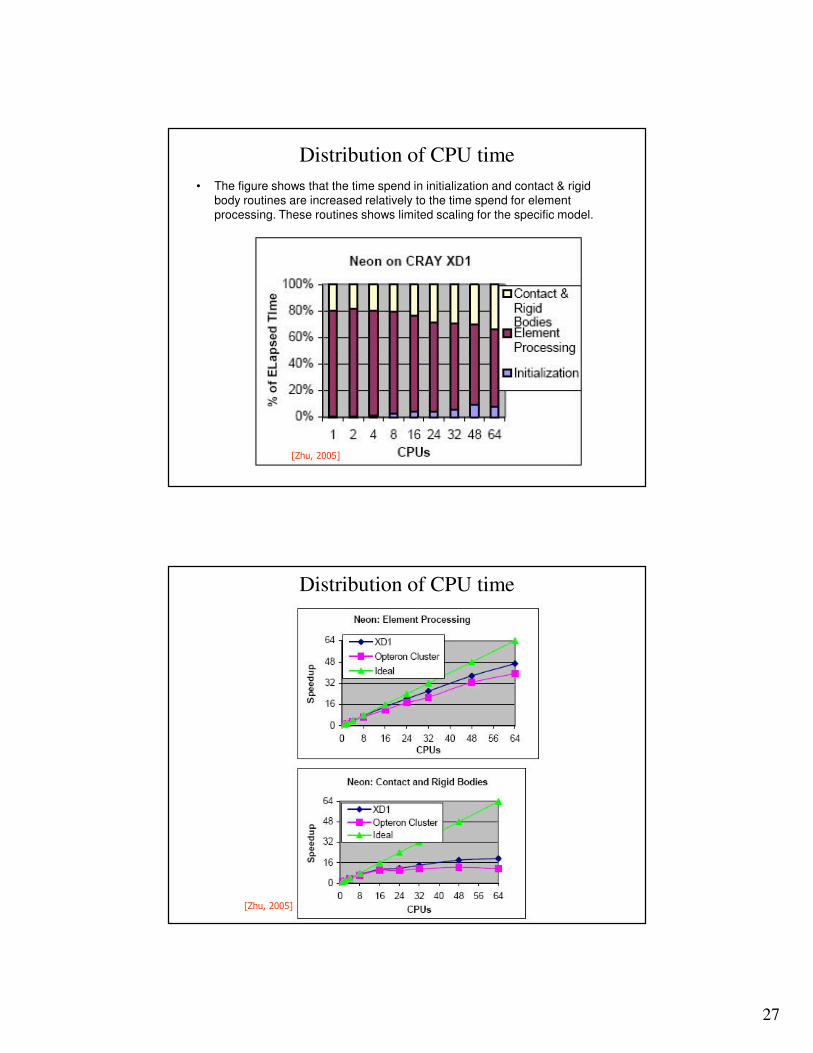
Distribution of CPU time
In order to investigate the scaling of different phases of the MPP run [Zhu, 2005] made runs with the Neon (and the 3 car) benchmark test. He
looked at 3 different phases of the run:
� Initialization: The time spend on reading the deck, allocate
memory, domain composition does not scale since this is done serial on 1 CPU. However, the time is relative small.
� Element Processing: The phase for element processing i.e., calculation of motion, forces, stresses etc. is almost perfect parallel and is one of the phases where most time is used.
� Contact and Rigid Bodies: The time spend in contact can also be significant depending of the problem. Both the contact and the rigid body
routines are scalable.
27
• The figure shows that the time spend in initialization and contact & rigid body routines are increased relatively to the time spend for element processing. These routines shows limited scaling for the specific model.
Distribution of CPU time
[Zhu, 2005]
Distribution of CPU time
[Zhu, 2005]
28
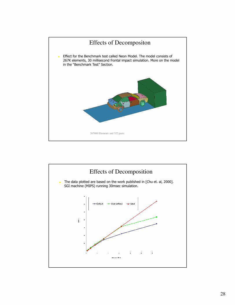
Effects of Decompositon
� Effect for the Benchmark test called Neon Model. The model consists of 267K elements, 30 millisecond frontal impact simulation. More on the model in the “Benchmark Test” Section.
267000 Elements and 322 parts.
Effects of Decomposition
� The data plotted are based on the work published in [Chu et. al, 2000]. SGI machine (MIPS) running 30msec simulation.
29
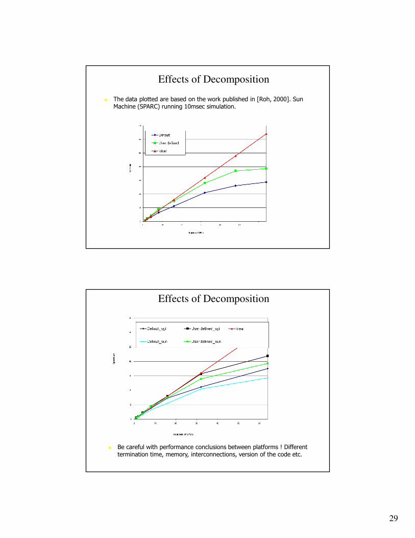
� The data plotted are based on the work published in [Roh, 2000]. Sun Machine (SPARC) running 10msec simulation.
Effects of Decomposition
Effects of Decomposition
� Be careful with performance conclusions between platforms ! Different termination time, memory, interconnections, version of the code etc.
30
Summary
� During the years LSTC has tested many different set-up for MPP. As shown there are many potential parameters that influence the scaling of the MPP code. Some of the most important ones are:
� Decomposition (user controlled)
� Memory/Cache System
� Interconnections
� MPI (2009: more or less same performance)
� Compiler (not user controlled)
Special Decomposition
31
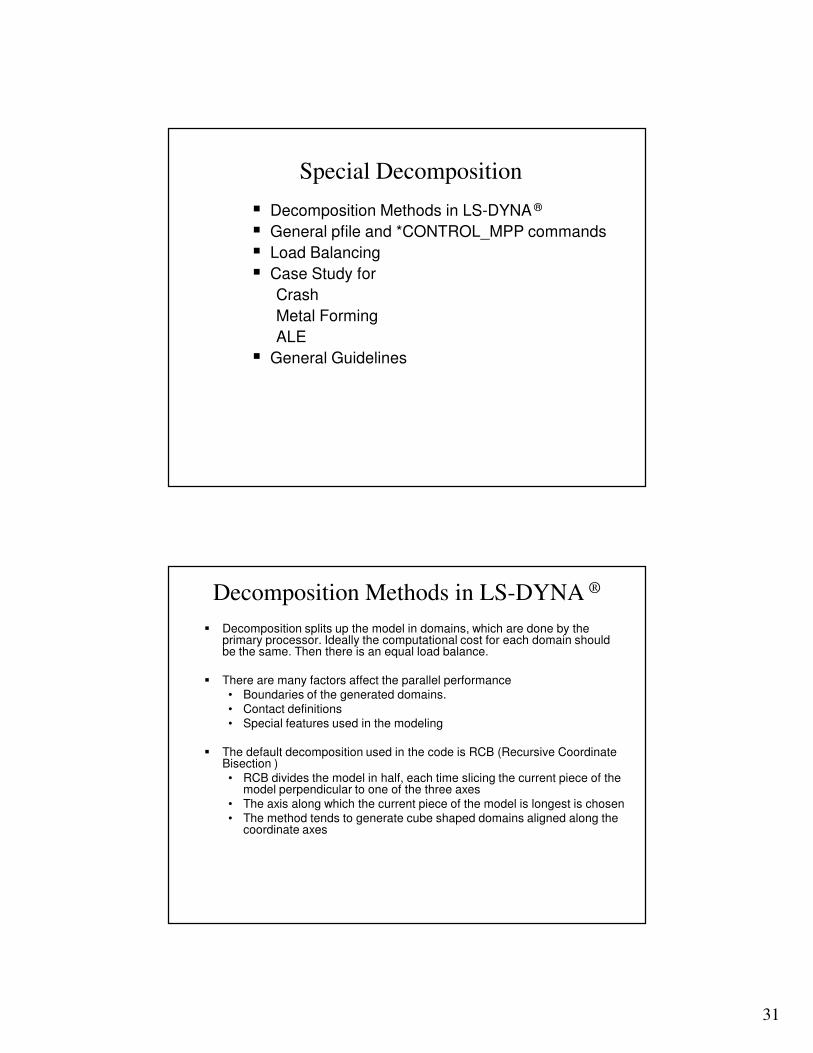
Special Decomposition
� Decomposition Methods in LS-DYNA ®
� General pfile and *CONTROL_MPP commands
� Load Balancing
� Case Study for
Crash
Metal Forming
ALE
� General Guidelines
� Decomposition splits up the model in domains, which are done by the primary processor. Ideally the computational cost for each domain should be the same. Then there is an equal load balance.
� There are many factors affect the parallel performance • Boundaries of the generated domains.
• Contact definitions• Special features used in the modeling
� The default decomposition used in the code is RCB (Recursive Coordinate Bisection )• RCB divides the model in half, each time slicing the current piece of the
model perpendicular to one of the three axes• The axis along which the current piece of the model is longest is chosen• The method tends to generate cube shaped domains aligned along the
coordinate axes
Decomposition Methods in LS-DYNA ®
32
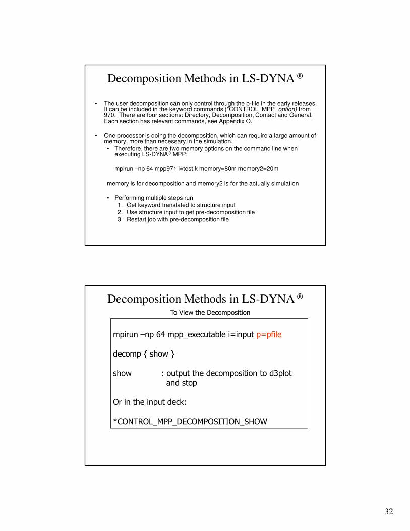
• The user decomposition can only control through the p-file in the early releases. It can be included in the keyword commands (*CONTROL_MPP_option) from 970. There are four sections: Directory, Decomposition, Contact and General. Each section has relevant commands, see Appendix O.
• One processor is doing the decomposition, which can require a large amount of memory, more than necessary in the simulation. • Therefore, there are two memory options on the command line when
executing LS-DYNA® MPP:
mpirun –np 64 mpp971 i=test.k memory=80m memory2=20m
memory is for decomposition and memory2 is for the actually simulation
• Performing multiple steps run1. Get keyword translated to structure input2. Use structure input to get pre-decomposition file3. Restart job with pre-decomposition file
Decomposition Methods in LS-DYNA ®
To View the Decomposition
mpirun –np 64 mpp_executable i=input p=pfile
decomp { show }
show : output the decomposition to d3plot and stop
Or in the input deck:
*CONTROL_MPP_DECOMPOSITION_SHOW
Decomposition Methods in LS-DYNA ®
33
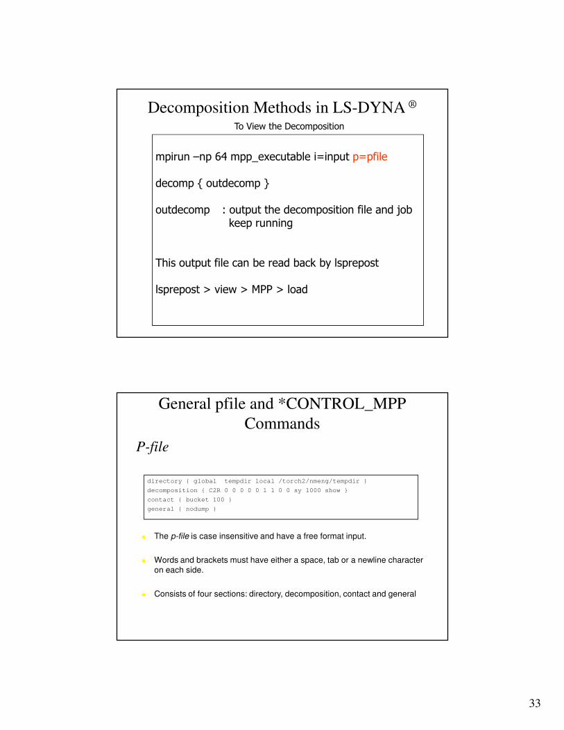
To View the Decomposition
mpirun –np 64 mpp_executable i=input p=pfile
decomp { outdecomp }
outdecomp : output the decomposition file and jobkeep running
This output file can be read back by lsprepost
lsprepost > view > MPP > load
Decomposition Methods in LS-DYNA ®
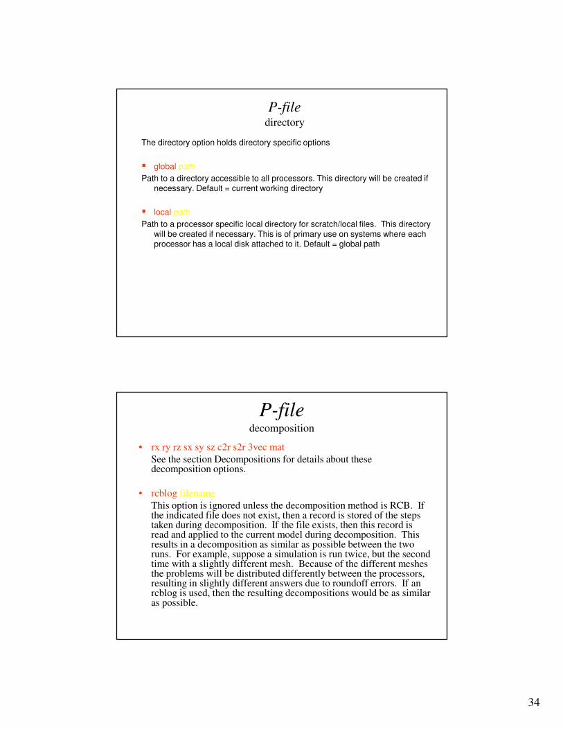
P-file
directory { global tempdir local /torch2/nmeng/tempdir }
decomposition { C2R 0 0 0 0 0 1 1 0 0 sy 1000 show }
contact { bucket 100 }
general { nodump }
� The p-file is case insensitive and have a free format input.
� Words and brackets must have either a space, tab or a newline character
on each side.
� Consists of four sections: directory, decomposition, contact and general
General pfile and *CONTROL_MPP
Commands
34
P-filedirectory
The directory option holds directory specific options
� global path
Path to a directory accessible to all processors. This directory will be created if necessary. Default = current working directory
� local path
Path to a processor specific local directory for scratch/local files. This directory will be created if necessary. This is of primary use on systems where each processor has a local disk attached to it. Default = global path
• rx ry rz sx sy sz c2r s2r 3vec mat
See the section Decompositions for details about these decomposition options.
• rcblog filename
This option is ignored unless the decomposition method is RCB. If the indicated file does not exist, then a record is stored of the steps taken during decomposition. If the file exists, then this record is read and applied to the current model during decomposition. This results in a decomposition as similar as possible between the two runs. For example, suppose a simulation is run twice, but the second time with a slightly different mesh. Because of the different meshes the problems will be distributed differently between the processors, resulting in slightly different answers due to roundoff errors. If an rcblog is used, then the resulting decompositions would be as similar as possible.
P-filedecomposition
35
• slist n1,n2,n3,...
This option changes the behavior of the decomposition in the following way. n1,n2,n3 must be a list of sliding interfaces occurring in the model (numbered according to the order in which they appear, starting with 1) delimited by commas and containing no spaces (eg "1,2,3" but not "1, 2, 3"). Then all elements belonging to the first interface listed will be distributed across all the processors. Next, elements belonging to the second listed interface will be distributed among all processors, and so on, until the remaining elements in the problem are distributed among the processors. Up to 5 interfaces can be listed. It is generally recommended that at most 1 or 2 interfaces be listed, and then only if they contribute substantially to the total computational cost. Use of this option can increase speed due to improved load balance.
• sidist n1,n2,n3,...
This is the opposite of the silist option: the indicated sliding interfaces are each forced to lie wholly on a single processor (perhaps a different one for each interface). This can improve speed for very small interfaces by reducing sychronization between the processors.
P-filedecomposition
P-filegeneral
The general option holds general options.
• nodump
If this keyword appears, all restart dump file writing will be suppressed
• nofull
If this keyword appears, writing of d3full (full deck restart) files will be suppressed.
36
P-file
There are many more option and correspondent *COTROL_MPP keyword.
Please check the User’s Manual Appendix O
� Different element formulation (minor)
� Force summation over shared nodes (minor)� Contact or coupling definitions (major)
Load Balancing
37
Main Loop
$ $ $ $
MPP
LAN
Process Elements
Contact
Constraints
Update Nodes
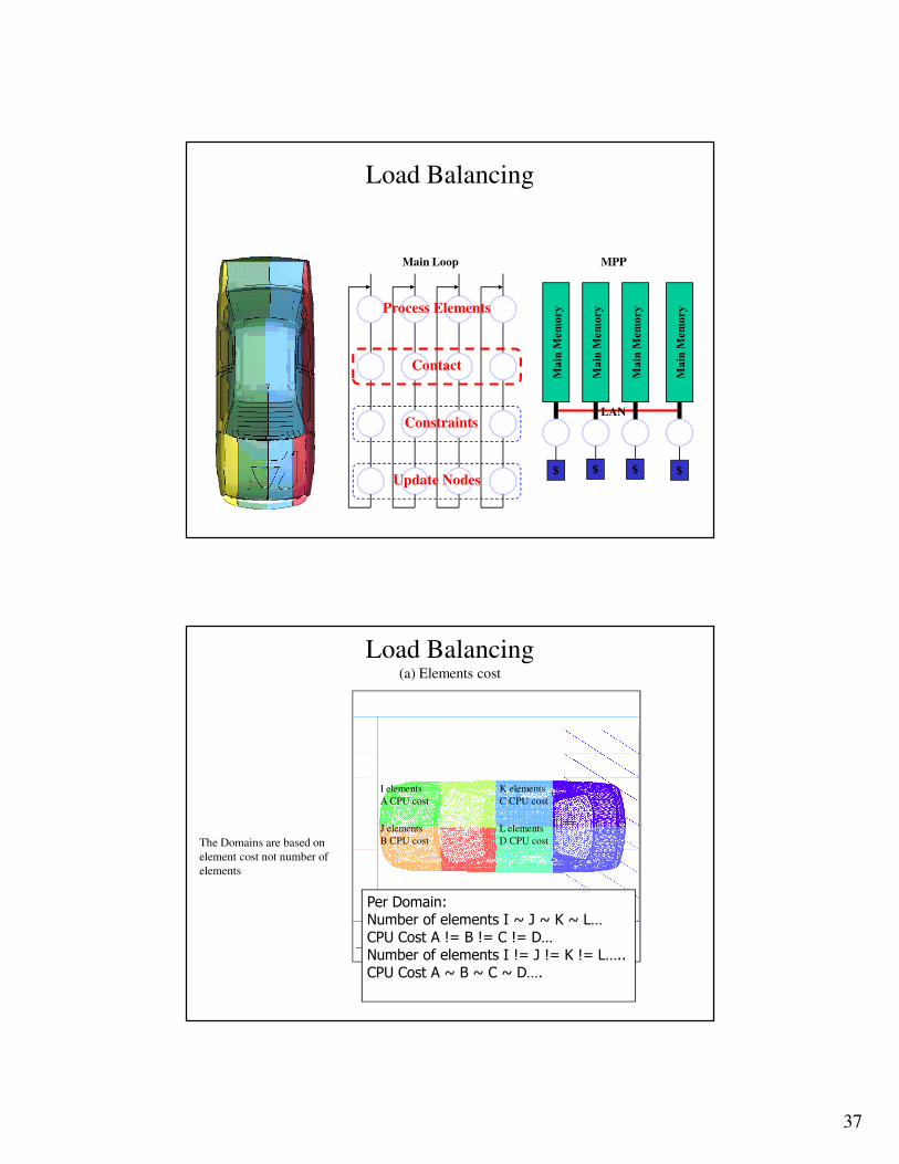
Load Balancing
I elements
A CPU cost
K elements
C CPU cost
L elements
D CPU cost
J elements
B CPU cost
Per Domain:Number of elements I ~ J ~ K ~ L…CPU Cost A != B != C != D…Number of elements I != J != K != L…..CPU Cost A ~ B ~ C ~ D….
The Domains are based on
element cost not number of
elements
Load Balancing(a) Elements cost
38
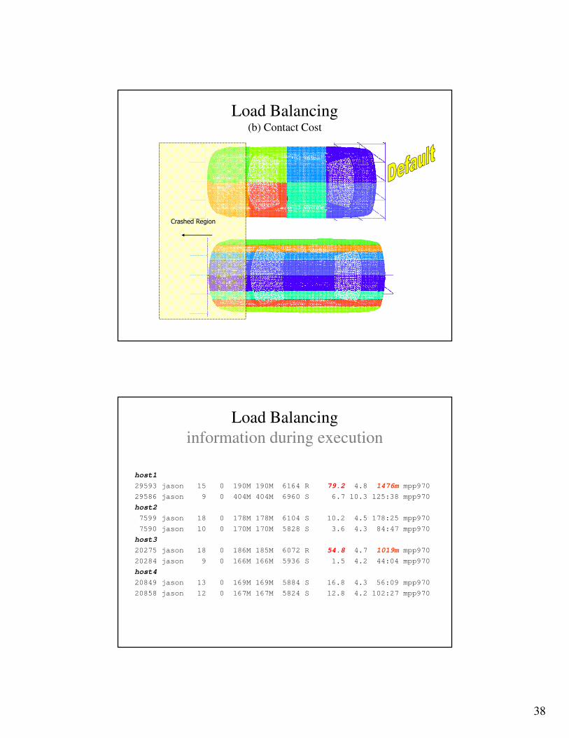
Crashed Region
Load Balancing(b) Contact Cost
host1
29593 jason 15 0 190M 190M 6164 R 79.2 4.8 1476m mpp970
29586 jason 9 0 404M 404M 6960 S 6.7 10.3 125:38 mpp970
host2
7599 jason 18 0 178M 178M 6104 S 10.2 4.5 178:25 mpp970
7590 jason 10 0 170M 170M 5828 S 3.6 4.3 84:47 mpp970
host3
20275 jason 18 0 186M 185M 6072 R 54.8 4.7 1019m mpp970
20284 jason 9 0 166M 166M 5936 S 1.5 4.2 44:04 mpp970
host4
20849 jason 13 0 169M 169M 5884 S 16.8 4.3 56:09 mpp970
20858 jason 12 0 167M 167M 5824 S 12.8 4.2 102:27 mpp970
Load Balancing
information during execution
39
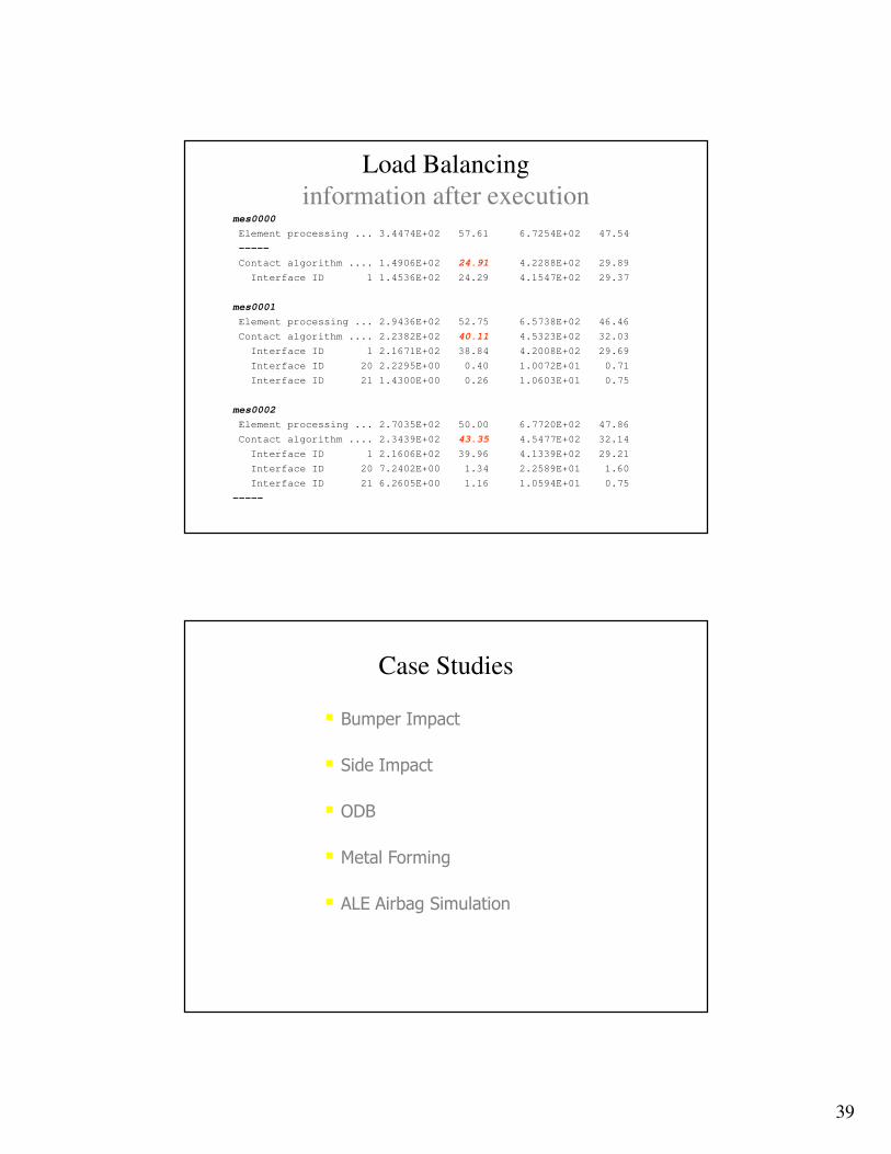
mes0000
Element processing ... 3.4474E+02 57.61 6.7254E+02 47.54
-----
Contact algorithm .... 1.4906E+02 24.91 4.2288E+02 29.89
Interface ID 1 1.4536E+02 24.29 4.1547E+02 29.37
mes0001
Element processing ... 2.9436E+02 52.75 6.5738E+02 46.46
Contact algorithm .... 2.2382E+02 40.11 4.5323E+02 32.03
Interface ID 1 2.1671E+02 38.84 4.2008E+02 29.69
Interface ID 20 2.2295E+00 0.40 1.0072E+01 0.71
Interface ID 21 1.4300E+00 0.26 1.0603E+01 0.75
mes0002
Element processing ... 2.7035E+02 50.00 6.7720E+02 47.86
Contact algorithm .... 2.3439E+02 43.35 4.5477E+02 32.14
Interface ID 1 2.1606E+02 39.96 4.1339E+02 29.21
Interface ID 20 7.2402E+00 1.34 2.2589E+01 1.60
Interface ID 21 6.2605E+00 1.16 1.0594E+01 0.75
-----
Load Balancing
information after execution
� Bumper Impact
� Side Impact
� ODB
� Metal Forming
� ALE Airbag Simulation
Case Studies
40
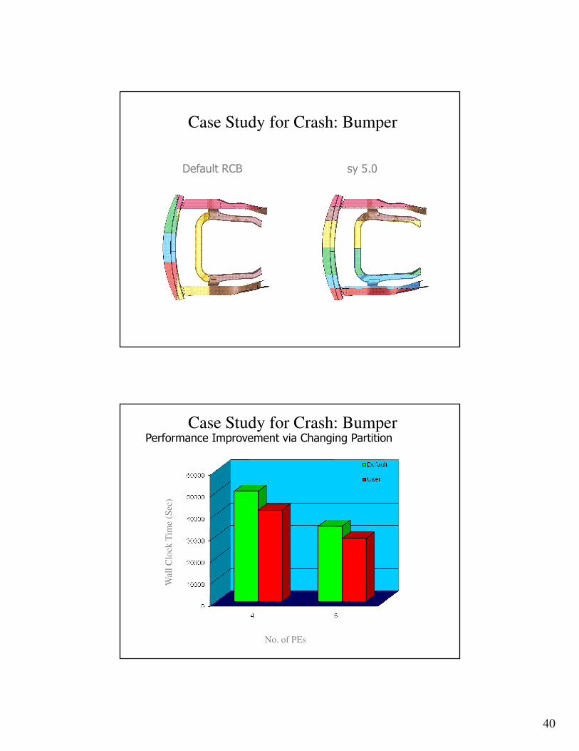
Case Study for Crash: Bumper
Default RCB sy 5.0
Performance Improvement via Changing Partition
No. of PEs
Wal
l C
lock
Tim
e (S
ec)
Case Study for Crash: Bumper
41
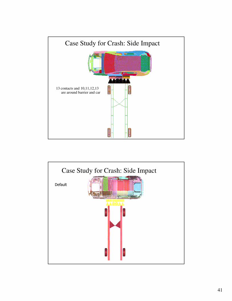
13 contacts and 10,11,12,13 are around barrier and car
Case Study for Crash: Side Impact
Default
Case Study for Crash: Side Impact
42
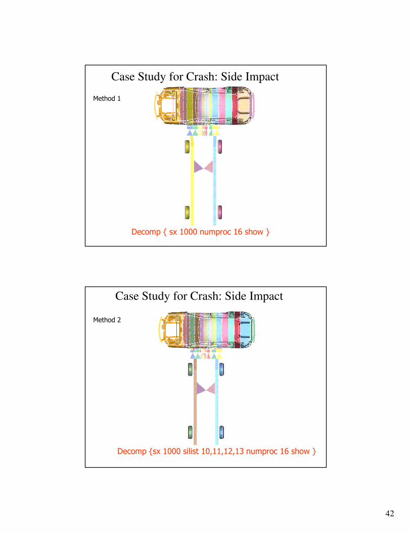
Method 1
Decomp { sx 1000 numproc 16 show }
Case Study for Crash: Side Impact
Decomp {sx 1000 silist 10,11,12,13 numproc 16 show }
Method 2
Case Study for Crash: Side Impact
43
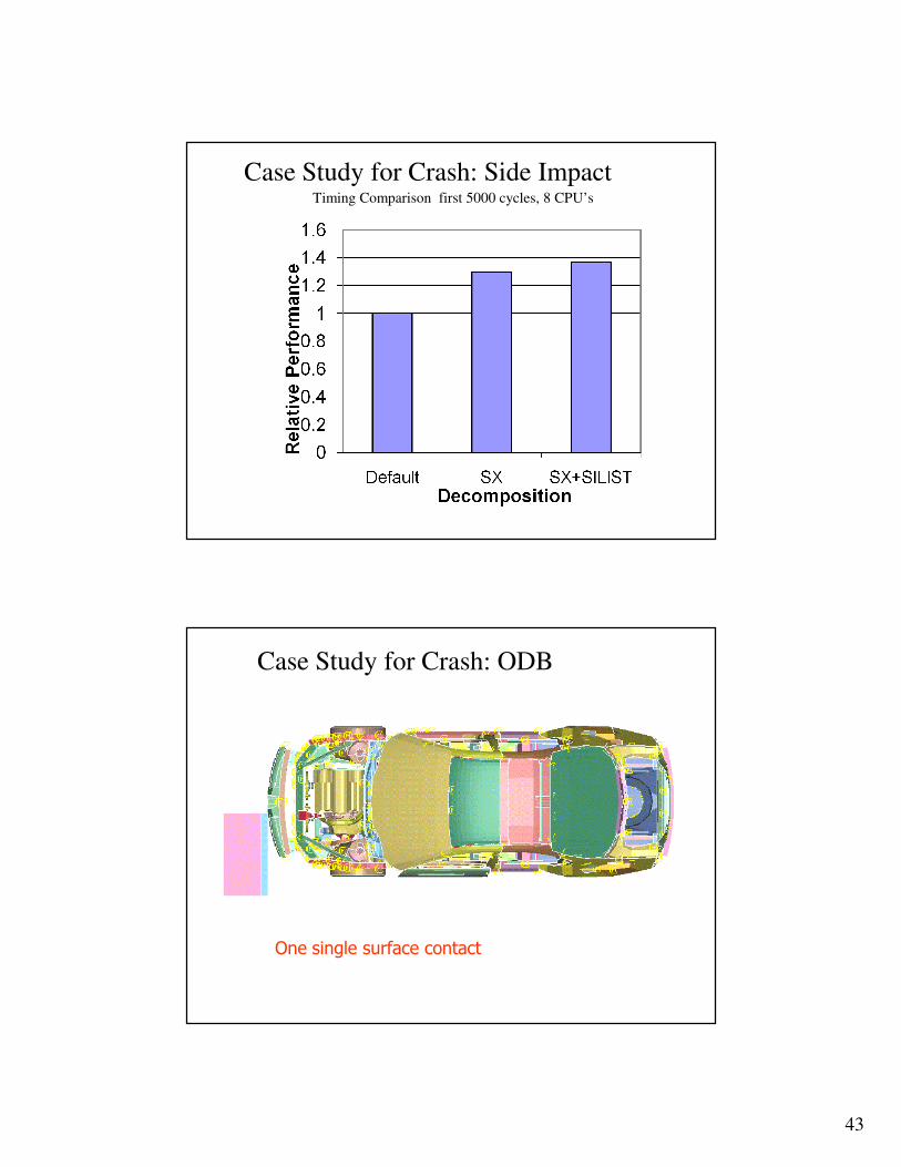
Timing Comparison first 5000 cycles, 8 CPU’s
Case Study for Crash: Side Impact
One single surface contact
Case Study for Crash: ODB
44
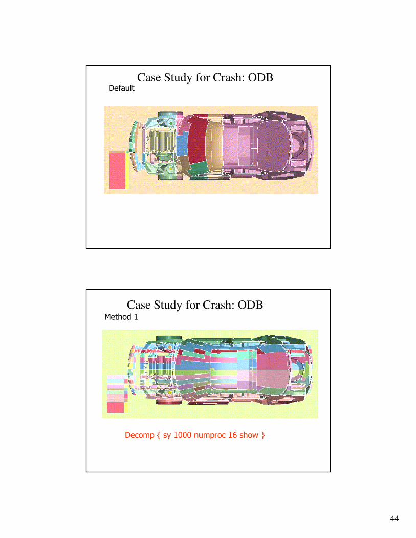
DefaultCase Study for Crash: ODB
Method 1
Decomp { sy 1000 numproc 16 show }
Case Study for Crash: ODB
45
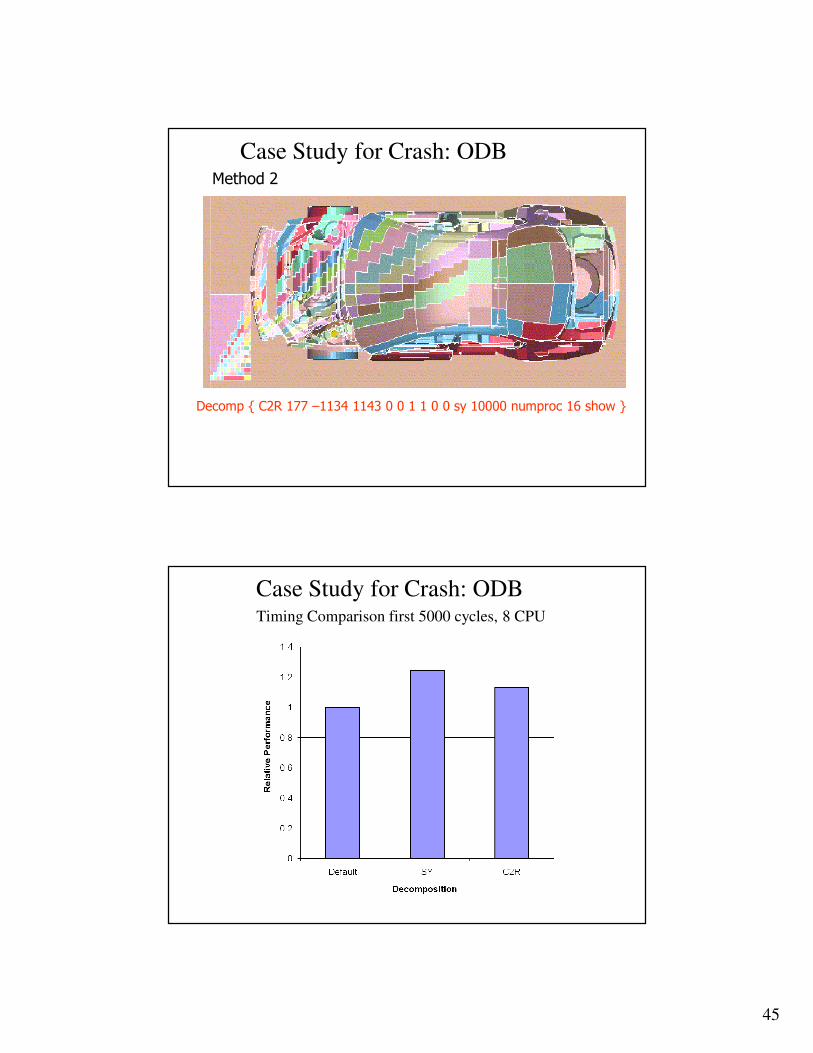
Method 2
Decomp { C2R 177 –1134 1143 0 0 1 1 0 0 sy 10000 numproc 16 show }
Case Study for Crash: ODB
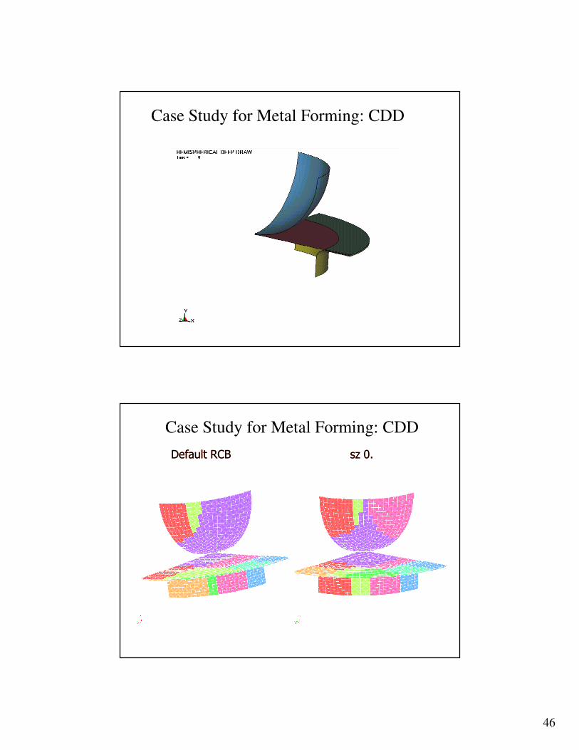
Timing Comparison first 5000 cycles, 8 CPU
Case Study for Crash: ODB
46
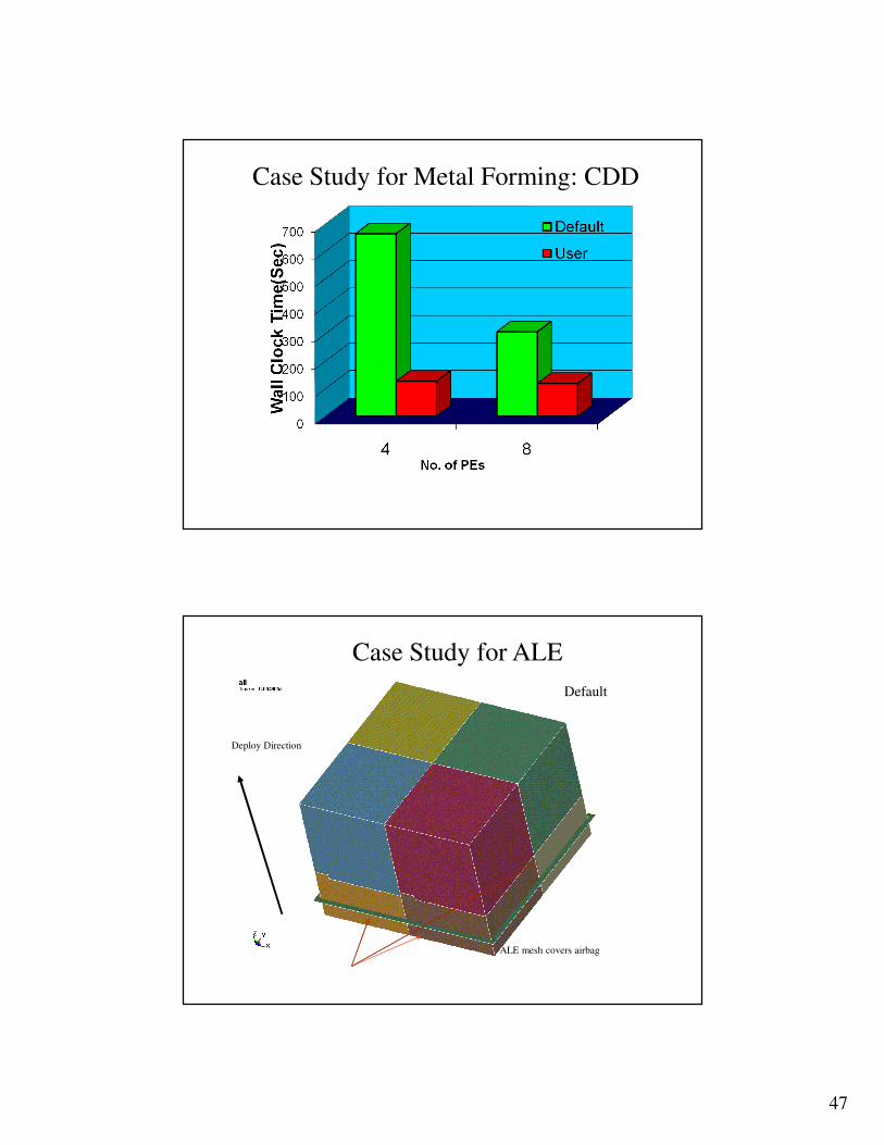
Case Study for Metal Forming: CDD
Default RCB sz 0.sz 0.Default RCB
Case Study for Metal Forming: CDD
47
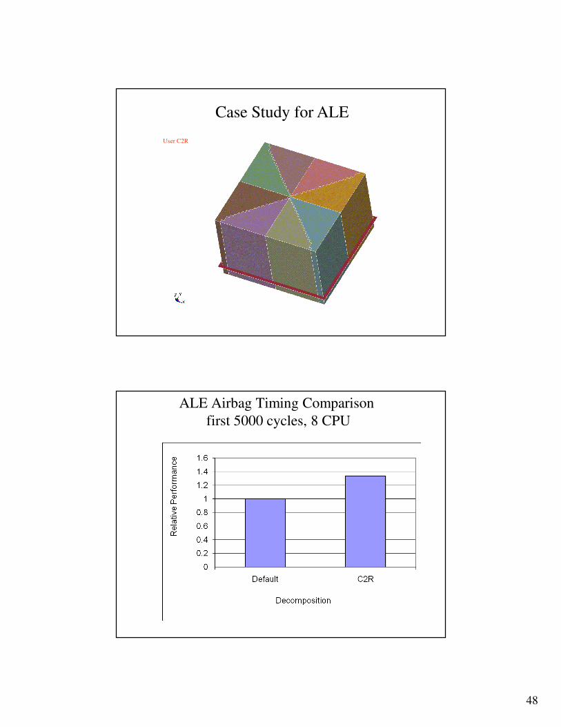
Case Study for Metal Forming: CDD
Case Study for ALE
Default
ALE mesh covers airbag
Deploy Direction
Only 4 CPU’s takes load in the beginning
48
Case Study for ALE
User C2R
ALE Airbag Timing Comparison
first 5000 cycles, 8 CPU
49
Better consistency
LSTC_REDUCE
� Results changes while changing from dual core to quad core system while using same number of MPP processors
RCBLOG
� Preserver the cut line for subsequent runs to reduce the decomposition noise
Special Features
General Guidelines
� For number of processors < 16, try to partition model along the direction of initial velocity (use e.g. automatic decomposition (*CONTROL_MPP_DECOMPOSITION_AUTO)
� Merge small contact definitions into big one
� Distribute large contact area evenly among processors via pfile
decomp { SILIST 1,2,3 }
Or in input deck
*CONTROL_MPP_DECOMPOSITION_CONTACT_DISTRIBUTE
� In forming simulation make the decomposition in the direction of the punch travel
� Please see more pfile options in Appendix O of the user manual The optimal decomposition is model and CPU depended.
50
MPP Contact
MPP Contact
� MPP Contact Algorithms
� MPP Contact Options
� Groupable Contact
� *CONTACT_FORCE_TRANSDUCER
� Contact General Guidelines
51
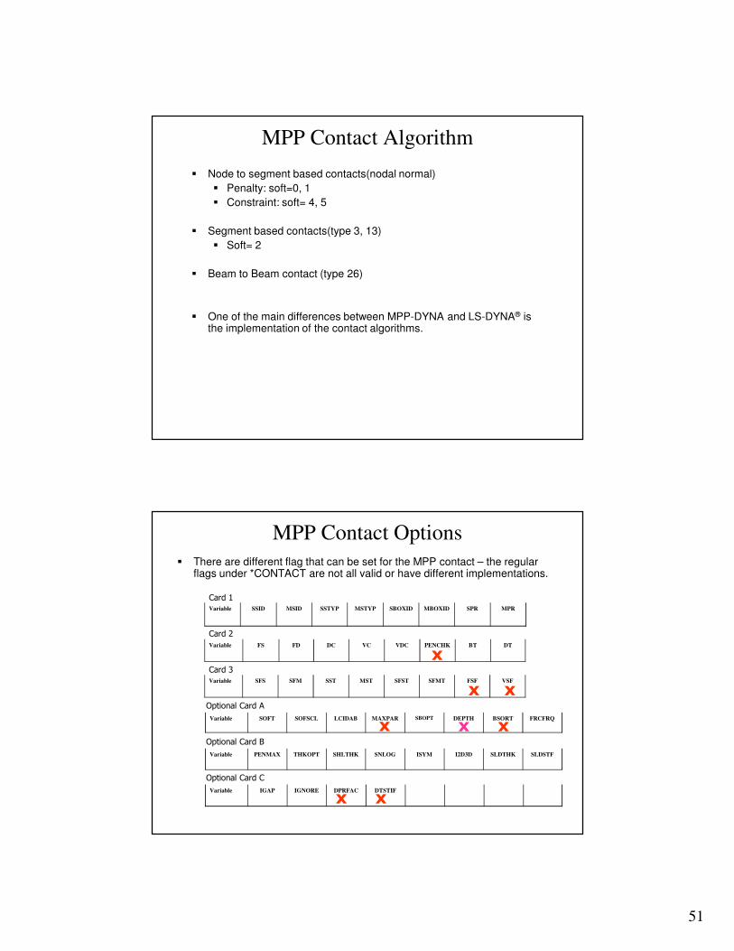
MPP Contact Algorithm
� Node to segment based contacts(nodal normal)
� Penalty: soft=0, 1
� Constraint: soft= 4, 5
� Segment based contacts(type 3, 13)
� Soft= 2
� Beam to Beam contact (type 26)
� One of the main differences between MPP-DYNA and LS-DYNA® is the implementation of the contact algorithms.
MPP Contact Options
� There are different flag that can be set for the MPP contact – the regular flags under *CONTACT are not all valid or have different implementations.
Variable SSID MSID SSTYP MSTYP SBOXID MBOXID SPR MPR
Variable FS FD DC VC VDC PENCHK BT DT
Variable SFS SFM SST MST SFST SFMT FSF VSF
x
x x
Card 1
Card 2
Card 3
Variable SOFT SOFSCL LCIDAB MAXPAR SBOPT DEPTH BSORT FRCFRQ
Variable PENMAX THKOPT SHLTHK SNLOG ISYM I2D3D SLDTHK SLDSTF
Variable IGAP IGNORE DPRFAC DTSTIF
xx
Optional Card A
Optional Card B
Optional Card C
xxx
52
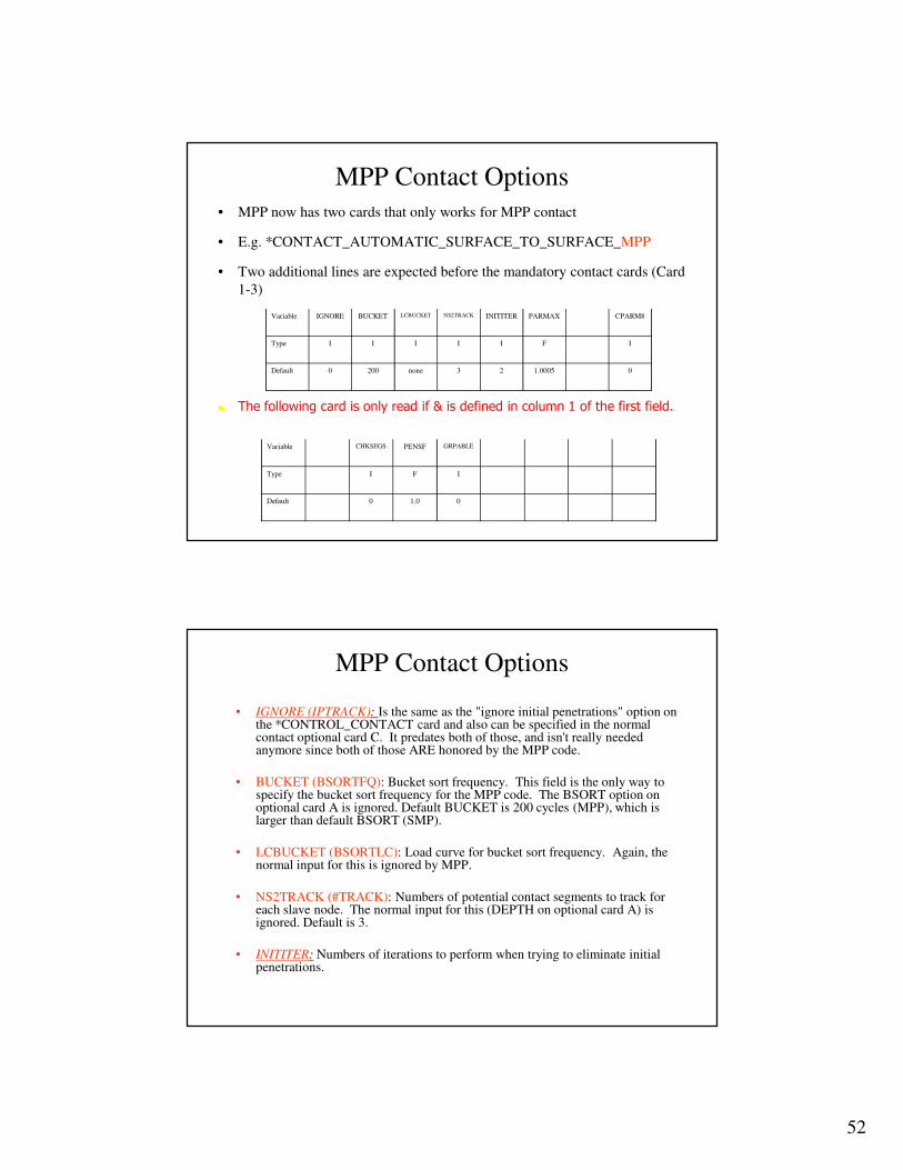
MPP Contact Options
• MPP now has two cards that only works for MPP contact
• E.g. *CONTACT_AUTOMATIC_SURFACE_TO_SURFACE_MPP
• Two additional lines are expected before the mandatory contact cards (Card
1-3)
Variable IGNORE BUCKET LCBUCKET NS2TRACK INITITER PARMAX CPARM8
Type I I I I I F I
Default 0 200 none 3 2 1.0005 0
� The following card is only read if & is defined in column 1 of the first field.
Variable CHKSEGS PENSF GRPABLE
Type I F I
Default 0 1.0 0
• IGNORE (IPTRACK): Is the same as the "ignore initial penetrations" option on the *CONTROL_CONTACT card and also can be specified in the normal contact optional card C. It predates both of those, and isn't really needed anymore since both of those ARE honored by the MPP code.
• BUCKET (BSORTFQ): Bucket sort frequency. This field is the only way to specify the bucket sort frequency for the MPP code. The BSORT option on optional card A is ignored. Default BUCKET is 200 cycles (MPP), which is larger than default BSORT (SMP).
• LCBUCKET (BSORTLC): Load curve for bucket sort frequency. Again, the normal input for this is ignored by MPP.
• NS2TRACK (#TRACK): Numbers of potential contact segments to track for each slave node. The normal input for this (DEPTH on optional card A) is ignored. Default is 3.
• INITITER: Numbers of iterations to perform when trying to eliminate initial penetrations.
MPP Contact Options
53
• PARMAX: The parametric extension distance for contact segments. The MAXPAR parameter on optional card A is not used. The default for PARMAX is 1.0005 (MPP) while the default for MAXPAR (SMP) is 1.025.
• CPARM8:
1: Exclude beam to beam contact from the same part ID. This is for *CONTACT_AUTOMATIC_GENERAL.
2: Consider Spotweld beams in contact
• CHKSEGS: Special element check is done and elements are removed from the contact, if the elements are badly shaped. Valid for SURFACE_TO_SURFACE and NODE_TO_SURFACE contacts.
• GRPABLE: This is still under development. It activates a new set of contacts that are faster and scales better that the regular contacts. Some contacts uses this option already when running MPP.
MPP Contact Options
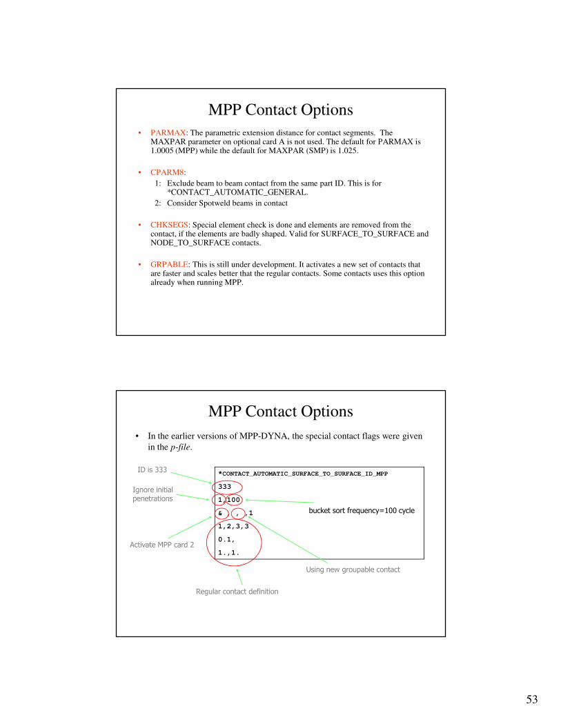
• In the earlier versions of MPP-DYNA, the special contact flags were given
in the p-file.
*CONTACT_AUTOMATIC_SURFACE_TO_SURFACE_ID_MPP
333
1,100
& , , ,1
1,2,3,3
0.1,
1.,1.
ID is 333
Ignore initial penetrations
Using new groupable contact
Activate MPP card 2
Regular contact definition
bucket sort frequency=100 cycle
MPP Contact Options
54
107
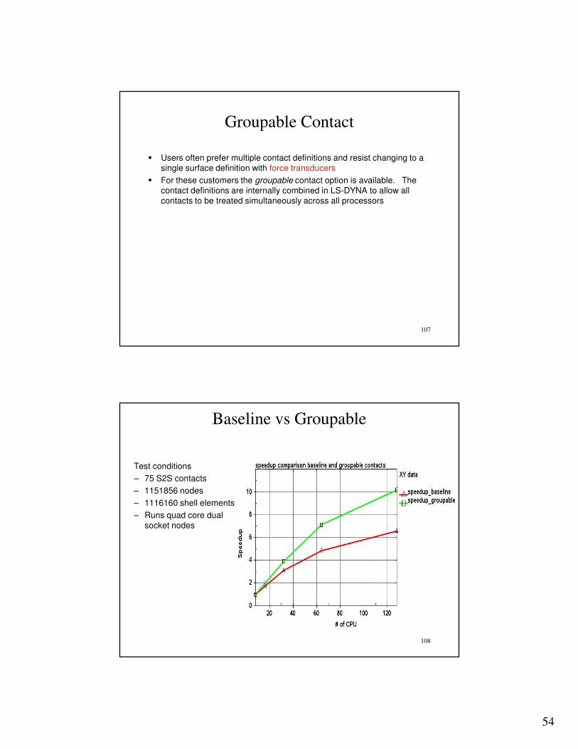
Groupable Contact
� Users often prefer multiple contact definitions and resist changing to a single surface definition with force transducers
� For these customers the groupable contact option is available. The contact definitions are internally combined in LS-DYNA to allow all contacts to be treated simultaneously across all processors
108
Baseline vs Groupable
Test conditions
– 75 S2S contacts
– 1151856 nodes
– 1116160 shell elements
– Runs quad core dual
socket nodes
55
109
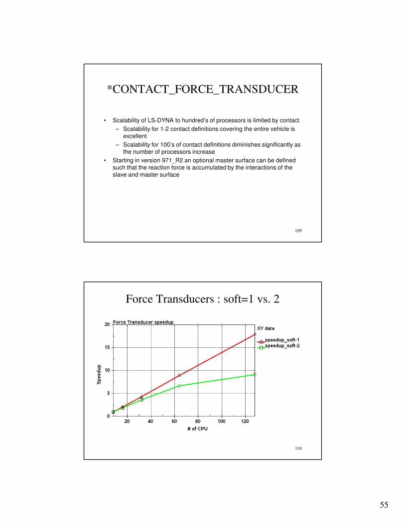
*CONTACT_FORCE_TRANSDUCER
• Scalability of LS-DYNA to hundred’s of processors is limited by contact
– Scalability for 1-2 contact definitions covering the entire vehicle is excellent
– Scalability for 100’s of contact definitions diminishes significantly as the number of processors increase
• Starting in version 971_R2 an optional master surface can be defined such that the reaction force is accumulated by the interactions of the slave and master surface
110
Force Transducers : soft=1 vs. 2
Force Transducer contact (one SSC added):
Elapsed time 8 proc 16 proc 32 proc 64 proc 128 proc
8313.00 4054.00 1933.00 925.00 464.00
Speedup 2.05 2.10 2.09 1.99
Speedup 4.30 4.38 4.17
Speedup 8.99 8.74
Speedup 17.92
56
� If changes is to be made to the contact, then use the cards in the input deck instead of the p-file.
� To isolate any given contact to a single processor, use *CONTROL_MPP_DECOMPOSITION_CONTACT_ISOLATE
� Forming contact in MPP is not meant to be used with solid elements (slave side). SMP may behave okay in such a case.
� BUCKET can be decreased to e.g. 100 if contact is not determined.
� *The ONE_WAY_SURFACE in MPP is similar to the SURFACE_TO_SURFACE contact in SMP.
� The use of *CONTACT_AUTOMATIC_SURFACE_TO_SURFACE with SOFT=2 will be the contact that will give most similar results between MPP-DYNA and SMP.
� It can be beneficial to use SOFT=2 for ERODING contact since the contact search is good.
Contact General Guidelines
General Guidelines
57
General Guidelines
� Numerical Consistency
� Debugging
� Cluster Tuning
� Pre-decomposition
� Restart
General Guidelines
�If error termination or unstable behavior occur, check for unsupported features. There is in general no error trap that indicates that a feature not is in MPP.
�12-32 processors is sometimes preferred for smaller models but the
optimal number of CPU’s strongly depends on the model.
�Single processor performance of LS-DYNA/MPP ~= LS-DYNA/SMP
�Will run efficiently with large contact definition – ease of modeling
�MPP is beneficial for more than 10k elements/processor
�If contact problems occur�Turn on IGNORE option�Try to use SOFT=2 at Optional card A.
58
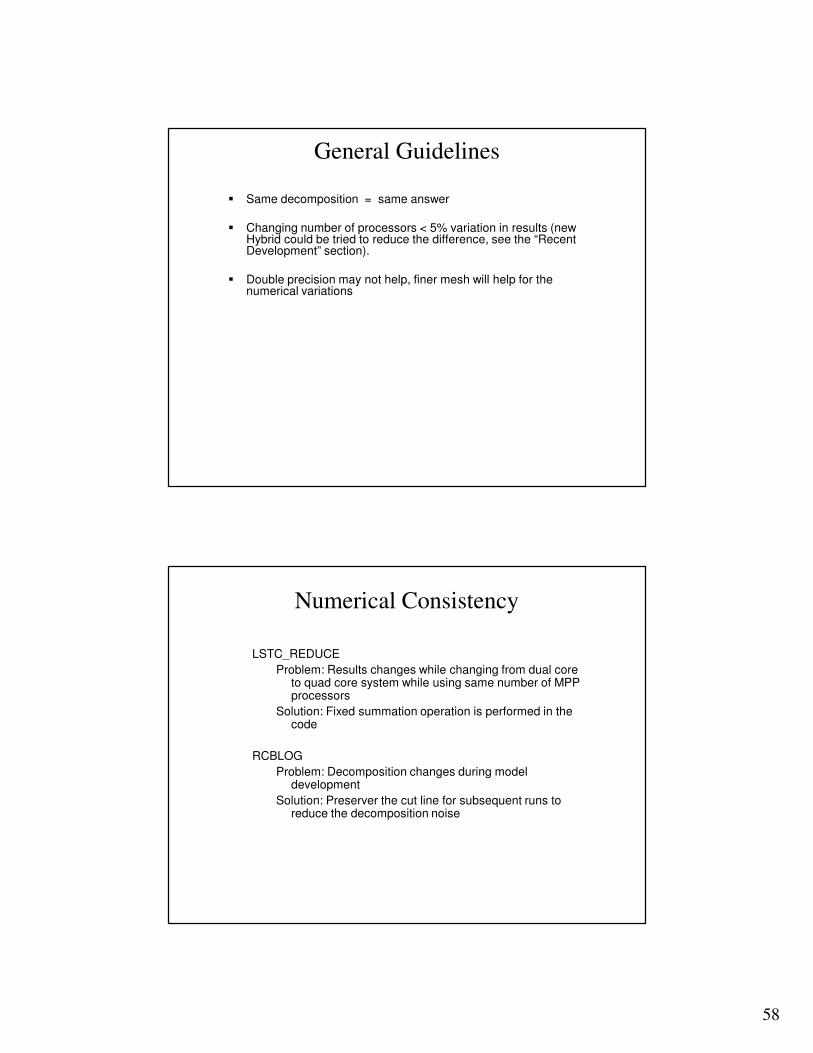
� Same decomposition = same answer
� Changing number of processors < 5% variation in results (new Hybrid could be tried to reduce the difference, see the “Recent Development” section).
� Double precision may not help, finer mesh will help for the numerical variations
General Guidelines
Numerical Consistency
LSTC_REDUCE
Problem: Results changes while changing from dual core to quad core system while using same number of MPP processors
Solution: Fixed summation operation is performed in the code
RCBLOG
Problem: Decomposition changes during model development
Solution: Preserver the cut line for subsequent runs to reduce the decomposition noise
59
Debugging• The error messages from MPP-DYNA can be different from LS-DYNA®
• To locate an error one often has to search each of the messag files mes#### in order to find any information. These files are written for each processor.
• The code will trap the segmentation violation (SEGV) and output the rank number. One could rerun the job and attach the debugger to the running thread and get the trace back map. This usually gives good information for changing input.
gdb path_to_mpp_code/mpp971 PID
> continue
SEGV
> where
• As for LS-DYNA® a debugger can be used if a core file is written:
gdb path_to_mpp_code/mpp971 core
• Type where to get more info and quit for exit
• Can indicate which subroutine is the problem and hence ease the model debugging.
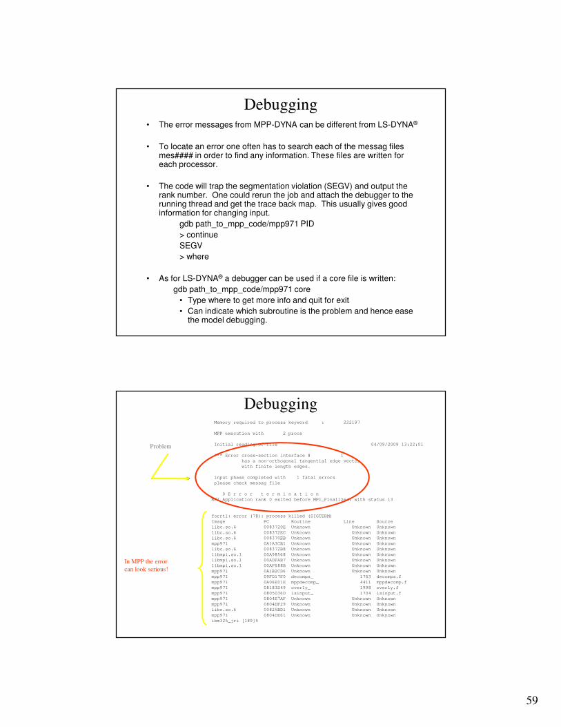
DebuggingMemory required to process keyword : 222197
MPP execution with 2 procs
Initial reading of file 04/09/2009 13:22:01
*** Error cross-section interface # 1
has a non-orthogonal tangential edge vector
with finite length edges.
input phase completed with 1 fatal errors
please check messag file
0 E r r o r t e r m i n a t i o n
MPI Application rank 0 exited before MPI_Finalize() with status 13
forrtl: error (78): process killed (SIGTERM)
Image PC Routine Line Source
libc.so.6 0083720E Unknown Unknown Unknown
libc.so.6 008372EC Unknown Unknown Unknown
libc.so.6 008370EB Unknown Unknown Unknown
mpp971 0A1A3CB1 Unknown Unknown Unknown
libc.so.6 008372B8 Unknown Unknown Unknown
libmpi.so.1 00A98568 Unknown Unknown Unknown
libmpi.so.1 00ADFAB7 Unknown Unknown Unknown
libmpi.so.1 00AF688B Unknown Unknown Unknown
mpp971 0A1B2CD6 Unknown Unknown Unknown
mpp971 09FD17F0 decomps_ 1763 decomps.f
mpp971 0A06E01E mppdecomp_ 4411 mppdecomp.f
mpp971 08183D49 overly_ 1998 overly.f
mpp971 0805036D lsinput_ 1704 lsinput.f
mpp971 0804E7AF Unknown Unknown Unknown
mpp971 0804DF29 Unknown Unknown Unknown
libc.so.6 00825BD1 Unknown Unknown Unknown
mpp971 0804DE61 Unknown Unknown Unknown
ibm325_jri [189]%
Problem
In MPP the error
can look serious!
60
Debugging
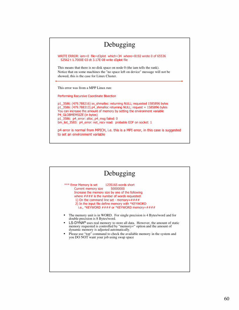
WRITE ERROR: iam=0 file=d3plot which=34 where=8192 wrote 0 of 6553652562 t 1.7000E-03 dt 3.17E-08 write d3plot file
This means that there is no disk space on node 0 (the iam tells the rank).
Notice that on some machines the "no space left on device" message will not be
showed, this is the case for Linux Cluster.
This error was from a MPP Linux run:
Performing Recursive Coordinate Bisection
p1_3586: (479.788216) xx_shmalloc: returning NULL; requested 1585896 bytesp1_3586: (479.788313) p4_shmalloc returning NULL; request = 1585896 bytesYou can increase the amount of memory by setting the environment variableP4_GLOBMEMSIZE (in bytes)p1_3586: p4_error: alloc_p4_msg failed: 0bm_list_3583: p4_error: net_recv read: probable EOF on socket: 1
p4 error is normal from MPICH, i.e. this is a MPI error, in this case is suggestedto set an environment variable
Debugging
*** Error Memory is set 1235165 words shortCurrent memory size 50000000Increase the memory size by one of the following where #### is the number of words requested: 1) On the command line set - memory=#### 2) In the input file define memory with *KEYWORDi.e., *KEYWORD #### or *KEYWORD memory=####
� The memory unit is in WORD. For single precision is 4 Bytes/word and for double precision is 8 Bytes/word.
� LS-DYNA® uses real memory to store all data. However, the amount of static memory requested is controlled by “memory=“ option and the amount of dynamic memory is adjusted automatically.
� Please use “top” command to check the available memory in the system and you DO NOT want your job using swap space
61
Cluster Tuning
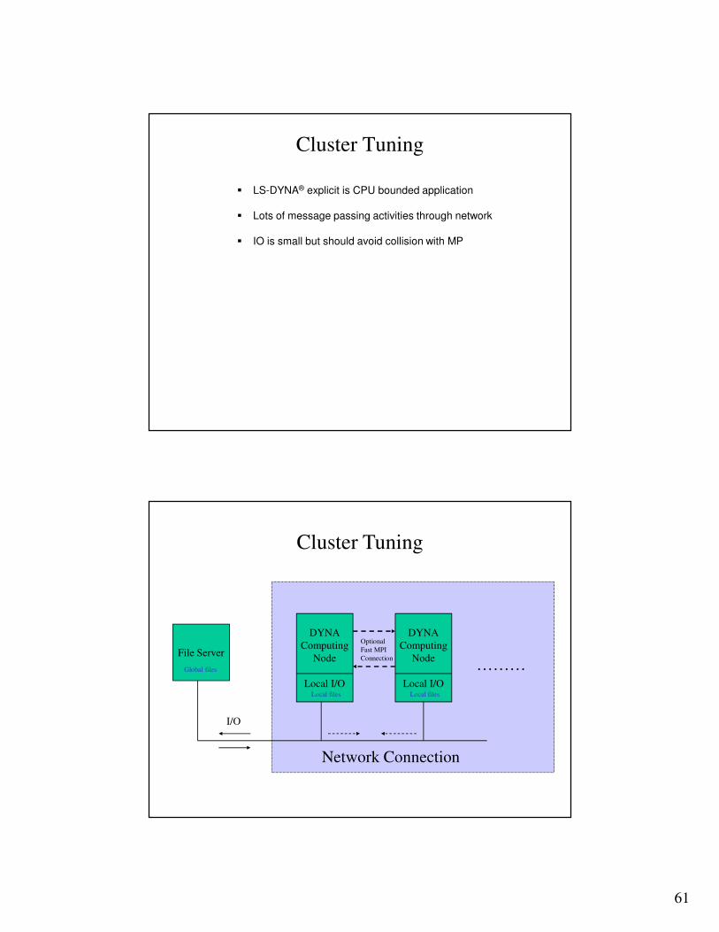
� LS-DYNA® explicit is CPU bounded application
� Lots of message passing activities through network
� IO is small but should avoid collision with MP
Cluster Tuning
File Server
………
Network Connection
DYNA
Computing
Node
Local I/O
DYNA
Computing
Node
Local I/O
I/O
Optional
Fast MPI
Connection
Local files
Global files
Local files
62
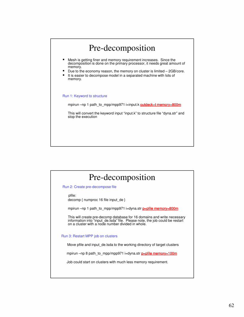
Pre-decomposition� Mesh is getting finer and memory requirement increases. Since the
decomposition is done on the primary processor, it needs great amount of memory.
� Due to the economy reason, the memory on cluster is limited – 2GB/core.� It is easier to decompose model in a separated machine with lots of
memory.
Run 1: Keyword to structure
mpirun –np 1 path_to_mpp/mpp971 i=input.k outdeckoutdeck=t memory=800m=t memory=800m
This will convert the keyword input “input.k” to structure file “dyna.str” and stop the execution
Pre-decompositionRun 2: Create pre-decompose file
pfile: decomp { numproc 16 file input_de }
mpirun –np 1 path_to_mpp/mpp971 i=dyna.str p=p=pfilepfile memory=800mmemory=800m
This will create pre-decomp database for 16 domains and write necessary information into “input_de.lsda” file. Please note, the job could be restart on a cluster with a node number divided in whole.
Run 3: Restart MPP job on clusters
Move pfile and input_de.lsda to the working directory of target clusters
mpirun –np 8 path_to_mpp/mpp971 i=dyna.str p=p=pfilepfile memory=100mmemory=100m
Job could start on clusters with much less memory requirement.
63
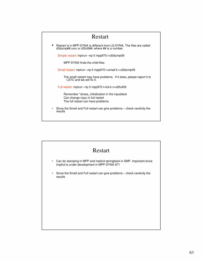
Restart
� Restart is in MPP-DYNA is different from LS-DYNA, The files are called d3dump##.xxxx or d3fulll##, where ## is a number.
Simple restart: mpirun –np 5 mpp970 r=d3dump09
MPP-DYNA finds the child files
Small restart: mpirun –np 5 mpp970 i=small.k r=d3dump09
The small restart may have problems. If it does, please report it to LSTC and we will fix it.
Full restart: mpirun –np 5 mpp970 i=full.k n=d3full09
Remember *stress_initialization in the inputdeckCan change ncpu in full restartThe full restart can have problems
• Since the Small and Full restart can give problems – check carefully the results
Restart
• Can do stamping in MPP and implicit springback in SMP. Important since implicit is under development in MPP-DYNA 971
• Since the Small and Full restart can give problems – check carefully the results
64
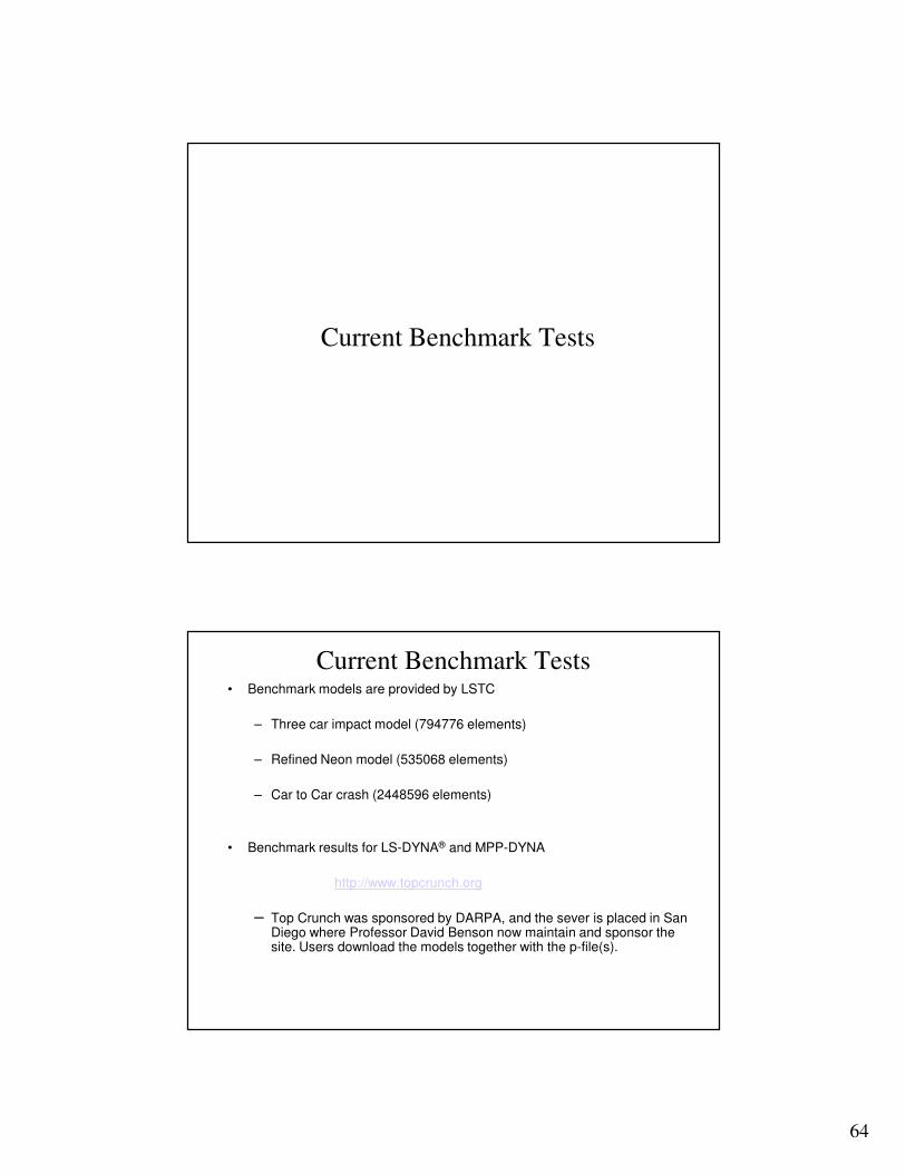
Current Benchmark Tests
Current Benchmark Tests• Benchmark models are provided by LSTC
– Three car impact model (794776 elements)
– Refined Neon model (535068 elements)
– Car to Car crash (2448596 elements)
• Benchmark results for LS-DYNA® and MPP-DYNA
http://www.topcrunch.org
– Top Crunch was sponsored by DARPA, and the sever is placed in San Diego where Professor David Benson now maintain and sponsor the site. Users download the models together with the p-file(s).
65
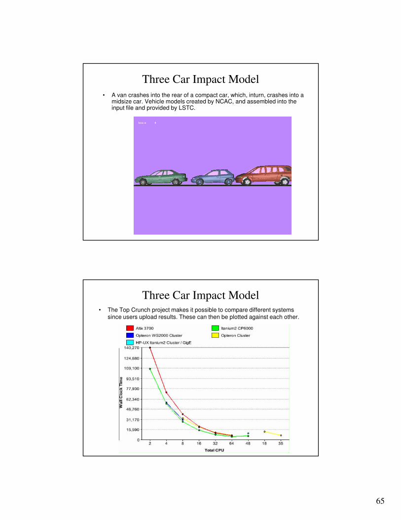
Three Car Impact Model
• A van crashes into the rear of a compact car, which, inturn, crashes into a midsize car. Vehicle models created by NCAC, and assembled into the input file and provided by LSTC.
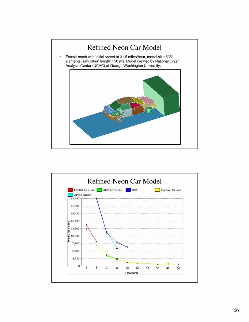
Three Car Impact Model• The Top Crunch project makes it possible to compare different systems
since users upload results. These can then be plotted against each other.
66
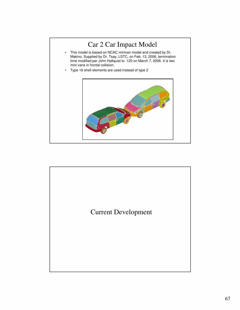
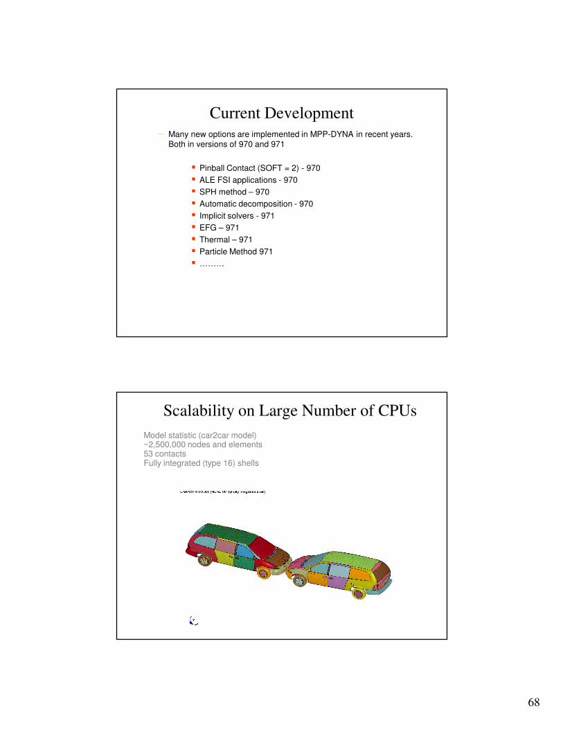
Refined Neon Car Model• Frontal crash with initial speed at 31.5 miles/hour, model size 535k
elements, simulation length: 150 ms. Model created by National Crash Analysis Center (NCAC) at George Washington University.
Refined Neon Car Model
67
Car 2 Car Impact Model• This model is based on NCAC minivan model and created by Dr.
Makino. Supplied by Dr. Tsay, LSTC, on Feb. 13, 2006, termination time modified per John Hallquist to .120 on March 7, 2006. It is two mini vans in frontal collision.
• Type 16 shell elements are used instead of type 2
Current Development
68
Current Development– Many new options are implemented in MPP-DYNA in recent years.
Both in versions of 970 and 971
� Pinball Contact (SOFT = 2) - 970
� ALE FSI applications - 970
� SPH method – 970
� Automatic decomposition - 970
� Implicit solvers - 971
� EFG – 971
� Thermal – 971
� Particle Method 971
� ………
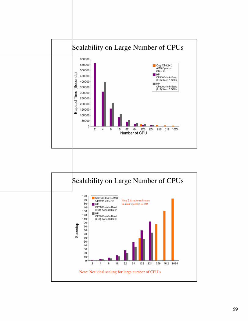
Scalability on Large Number of CPUs
Model statistic (car2car model)~2,500,000 nodes and elements53 contactsFully integrated (type 16) shells
69
2 4 8 16 32 64 128 224 256 512 10240
50000
100000
150000
200000
250000
300000
350000
400000
450000
500000
550000
600000
Cray XT4(2x1) AMD Opteron 2.6GHz
HP CP3000+InfiniBand (2x1) Xeon 3.0GHz
HP CP3000+InfiniBand (2x2) Xeon 3.0GHz
Number of CPU
Ela
pse
d T
ime
(S
eco
nd
s)
Scalability on Large Number of CPUs
2 4 8 16 32 64 128 224 256 512 10240
10
20
30
40
50
60
70
80
90
100
110
120
130
140
150
160
170Cray XT4(2x1) AMD Opteron 2.6GHz
HP CP3000+InfiniBand (2x1) Xeon 3.0GHz
HP CP3000+InfiniBand (2x2) Xeon 3.0GHz
Spe
edup
Here 2 is set to reference
So max speedup is 340
Scalability on Large Number of CPUs
Note: Not ideal scaling for large number of CPU’s
70
Multi-core/Multi-socket clusters
Scalability on Large Number of CPUs
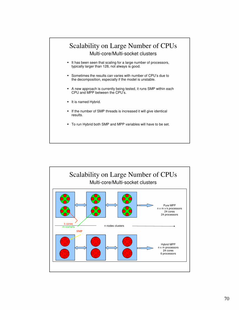
� It has been seen that scaling for a large number of processors, typically larger than 128, not always is good.
� Sometimes the results can varies with number of CPU’s due to the decomposition, especially if the model is unstable.
� A new approach is currently being tested, it runs SMP within each CPU and MPP between the CPU’s.
� It is named Hybrid.
� If the number of SMP threads is increased it will give identical results.
� To run Hybrid both SMP and MPP variables will have to be set.
n nodes clustersk cores
m sockets
Pure MPPn x m x k processors
24 cores24 processors
Hybrid MPPn x m processors
24 cores6 processors
Multi-core/Multi-socket clusters
Scalability on Large Number of CPUs
SMP
71
Multi-core/Multi-socket clusters
Scalability on Large Number of CPUs
� There is a special syntax that is required for the Hybrid approach.
� If e.g. the set-up is a system with 16 nodes, dual socket quad core system (as previous slide) the variable is:
� Set OMP_NUM_THREAD=4 (max four cores in each SMP)
� The system is a 128 core system
� Mpirun –np 32 mpp971_hybrid i=input ncpu=-1
� 32 MPP Processors (green circle) and 1 core in each which then is a total of 32 cores.
� Mpirun –np 32 mpp971_hybrid i=input ncpu=-2
� 32 Processors and 2 cores in each = 64 cores
� Mpirun –np 32 mpp971_hybrid i=input ncpu=-4
� Total of 128 cores is used
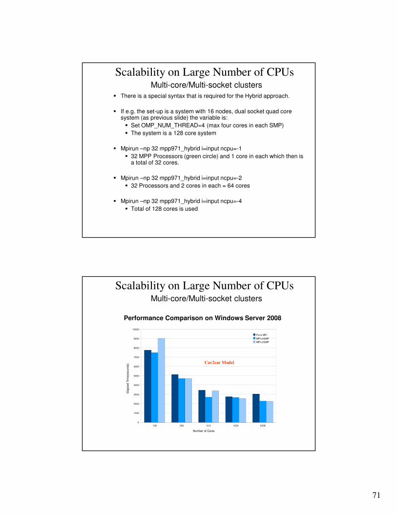
128 256 512 1024 2008
0
1000
2000
3000
4000
5000
6000
7000
8000
9000
10000
Pure MPI
MPI+4SMP
MPI+2SMP
Number of Cores
Ela
psed T
ime(s
econds)
Performance Comparison on Windows Server 2008
Multi-core/Multi-socket clusters
Scalability on Large Number of CPUs
Car2car Model
72
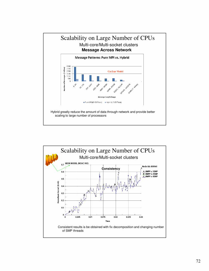
Message Across Network
Hybrid greatly reduce the amount of data through network and provide better scaling to large number of processors
Multi-core/Multi-socket clusters
Scalability on Large Number of CPUs
Car2car Model
Consistent results is be obtained with fix decomposition and changing number of SMP threads
Multi-core/Multi-socket clusters
Scalability on Large Number of CPUs
Consistency
73
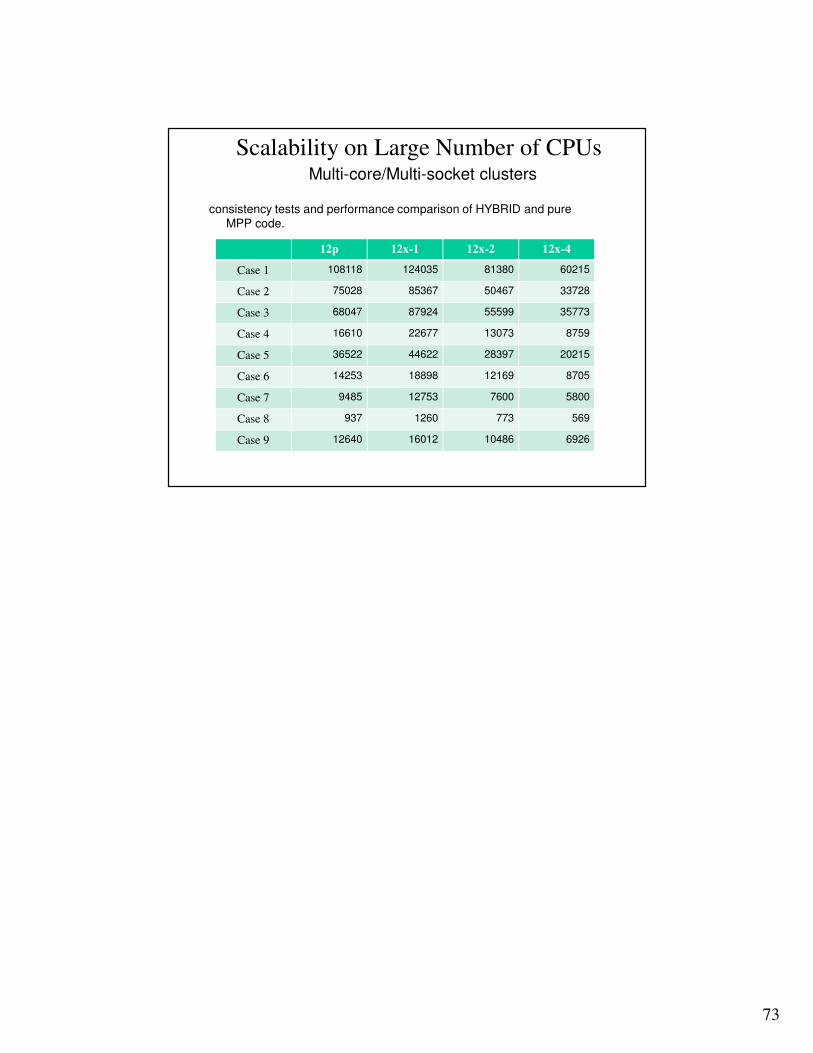
consistency tests and performance comparison of HYBRID and pure MPP code.
Multi-core/Multi-socket clusters
Scalability on Large Number of CPUs
12p 12x-1 12x-2 12x-4
Case 1 108118 124035 81380 60215
Case 2 75028 85367 50467 33728
Case 3 68047 87924 55599 35773
Case 4 16610 22677 13073 8759
Case 5 36522 44622 28397 20215
Case 6 14253 18898 12169 8705
Case 7 9485 12753 7600 5800
Case 8 937 1260 773 569
Case 9 12640 16012 10486 6926