AD-A11 6N NLTCLMTOSIN EMN AF 2/A SEPARATION MODEL FOR TWO-DIMENSIONAL AIRFOILS IN TRANSONI C FL--ETC(U)

UNLSIID JAN 82 F A D VORAK. D H CHOI 0AAG29-78-C-ORO

UNCLASSIFIED ARO-1586.2-E NL

7 EDA1 4 NAYIA H ODhIC EDh E F16h I/

TElEhEEEh

II . 117 1 111112.51. - l- IIII2

11. IIIIi2 I.f 1.8

MICROCOPY RESOLUTION TEST CHARI

NA I. NAI 1ll PH Al I

'TAN[DA,' 1C A : A

FINAL TECHNICAL REPORT

"A SEPARATION MODEL FOR

TWO-DIMENSIONAL AIRFOILS IN TRANSONIC FLOW"

DR. F.A. DVORAK

DR. D.H. CHOI

JANUARY 1982

PREPARED FOR:

DEPARTMENT OF THE ARMY

U.S. ARMY RESEARCH OFFICEP.O. Box 12211

RESEARCH TRIANGLE PARK, N.C. 27709

tINDER CONTRACT DAAG29-78-C-0004

PREPARED BY: 0

ANALYTICAL METHODS, INC.

2047 - 152ND AVENUE N.E.

REDMOND., WASHINGTON 98052 ((206) 643-9090

82 03 1 !5

Uncl assi fiedSECURITY CLASSIFICATION OF THIS PAGE (Mieni Date Entered)

PAGE READ INSTRUCTIONSREPORT DOCUMENTATION PAGEBEFORE COPLETING FORFinaO echcaleortFO•!. REPORT NUMBER -2. GOVT ACCESSION NO 3. RECI IENT'S CATALOG NUMBER

4. TITLE (ad Subtitle) S. TYPE OF REPORT & PERIOD COVERED

A Searation Model for Two-Dimensional Airfoils 15 Nov. 1978 - 30 Nov. 1981

in Transonic Flow 6. PERFORMING ORG. REPORT NUMBER

7. AUTHOR(a) S. CONTRACT OR GRANT NUMBERW)

Dr. Frank A. Dvorak DAAG29-78-C-0004Dr. D.H. Choi

S. PERFORMING ORGANIZATION NAME AND ADDRESS 10. PROGRAM ELEMENT, PROJECT. TASK

Analytical Methods, Inc. AREA & WORK UNIT NUMBERS

2047 - 152nd Avenue N.E.Redmond, Washington 98052

11. CONTROLIN(' OFFICE NAME AND ADDRESS 12. REPORT DATE

U.S. Army Research Office January 1982Post Office Box 12211 13. NUMBER OF PAGES

Research Trianale Park, N.C. 27709 38MONITORING AGENCY NAME & ADDRESS(f different from Controlling Office) IS. SECURITY CLASS. (of this report)

Unclassified

IS. DECLASSIFICATION/DOWNGRAOINGSCHEDULE

16. DISTRIBUTION STATEMENT (of thie Report)

Approved for public release; distribution unlimited.

17. DISTRIBUTION STATEMENT (of the ebetract entered In Block 20, It different from Report)

III. SUPPLEMENTARY NOTESThe view, opinions, and/or findings contained in this reort are those of the

author(s) and should not be construed as an official Department of the Armyposition, policy or decision, unless so designated by other documentation.

19. KEY WORDS (Continue on reveres, side If necessary and identify by block number)

separated flows; transonic flow; aerodynamic stall; viscous potential flowinteraction analysis

2& ATaRAcT (entiare - ,efeea ad t neweesen and idatly by block inbet)

A calculation method for transonic separated flow about two-dimensional air-foils at incidence is presented in this report. The method is capable ofpredicting the effects of both leading- and trailing-edge separated flows,although the former is usually associated with a complete collapse of the air-foil flow field, in which case the flow is no longer supercritical. A viscouspotential flow iteration procedure provides the connection between potentialflow, boundary layer and wake modules. The separated wake is modelled in the

D O" Wo 3 IrMITo OF I NOV 6 IS OILETED J 1 UnclassifiedSECUtTY CLASSIFICATION OF THIS PAGE (Wihen Date 1ntered

Itlna cci fiadSECUNITY CLASSIFICATION OF THIS PAGE( M-m Data RaleatQ

potential flow analysis by thin sheets across which exists a jump in velocitypotential. These sheets are analogous to vorticity sheets in incompressibleflow. The basic potential flow method is a modification of Jameson',s fullpotential method. Calculations for four different airfoils have been comparedwith experiment for pressure distributions as well as integrated forces. Theagreement between theory and experiment is generally good even when shockwaves are present.

UnclassifiedSECUITY CLASSIFICATION OF THIS PAGE(Wate Date Zftm*0

SUMMARY

A calculation method for transonic separated flow about two-dimensionalairfoils at incidence is presented in this report. The method is capableof predicting the effects of both leading- and trailing-edge separated flows,although the former is usually associated with a complete collapse of the air-foil flow field, in which case the flow is no longer supercritical. A viscouspotential flow iteration procedure provides the connection between potentialflow, boundary layer and wake modules. The separated wake is modelled in thepotential flow analysis by thin sheets across which exists a jump in velocitypotential. These sheets are analogous to vorticity sheets in incompressibleflow. The basic potential flow method is a modification of Jameson's fullpotential method. Calculations for four different airfoils have been comparedwith experiment for pressure distributions as well as integrated forces. Theagreement between theory and experiment is generally good even when shockwaves are present.

Accession For

NTIS tAH&

DTIC T

1o _I J , ! , , , .

By...

PREFACE

The work described in this technical report was performed by AnalyticalMethods, Inc. for the Department of the Army, U.S. Army Research Office,Research Triangle Park, North Carolina, under Contract DAAG29-78-C-0004.The research program was undertaken under the technical cognizance of Dr.Robert E. Singleton, Director, Engineering Sciences Division, U.S. ArmyResearch Office. Dr. Frank A. Dvorak was the Principal Investigator andthe Program Manager, and Dr. D.H. Choi was an Associate Investigator.

Analytical Methods, Inc. wishes to gratefully acknowledge the assistanceof Hughes Helicopters, Inc., Culver City, California, in providing realistichelicopter airfoil geometries for comparison with program TRANMAX.

2

TABLE OF CONTENTS

Section No. Title Page No.

SUMMARY ........... ................................. 1

PREFACE ............ ................................ 2

TABLE OF CONTENTS ............ .......................... 3

LIST OF ILLUSTRATIONS .......... .......................... 4

1.0 INTRODUCTION ........... ............................ 5

2.0 DESCRIPTION OF THE ANALYSIS METHOD

2.1 General Description ........ ...................... 7

2.2 Potential Flow Calculation Method

2.2.1 Basic Equations ........ .................... 72.2.2 MaDped Coordinate System ...... ................ 102.2.3 Inviscid Model of Separated Region .... ........... 122.2.4 Method of Solution ..... ................... ... 15

2.3 Calculation of Boundary Layer Development .... ........... 16

2.3.1 Cohen and Reshotko Method ...... ............... 162.3.2 Green's Method ........ .................... 18

3.0 RESULTS AND DISCUSSION ........ ....................... 20

4.0 CONCLUSIONS ........... ............................ 37

5.0 REFERENCES ........ ............................. .. 38

3

LIST OF ILLUSTRATIONS

Fig. No. Title Page No.

1 Calculation Procedure .. .. ... . . ... ..... ..... 8

2 Grid System. .. .. .. .. ... .. ... .. ... ..... 10

3 Wake Model .. .. ... .. ... .. ... .. ... ..... 12

4 Separated Region in the Computational Plane .. . ... .... 13

5 Finite-Difference Grid. .. . .. ... .... . .... ... 14

6(a), (b), (c) Pressure Distribution along GA(W)-l Airfoil . . . .21-23

7 C~ a Curve for GA(W)-l Airfoil. .. . ... .. ... .... 24

8(a), (b), (c) Pressure Distribution along a NACA 0012. .. .... 25-27

9 C~ a Curve for NACA 0012 Airfoil. .. . .... . ....... 28

10(a), (b), (c) Pressure Distribution along a Hughes Helicopters 29-31Company Airfoil .. . ... . .. . . . . . .. . .. . ..

11 C~ a Curve for a Hug~hes Helicopters Company Airfoil. . .. 32

12 Pressure Distribution along an Al Airfoil for M~ = 0.496;a8.5 . . . . . . . . . . . . . . . . . . . . . . . . . . . . . 34

13 Pressure Distribution along an Al Airfoil for M. 0.596;a = 6 .. . . . . . . . . . . . . . . . . . . . . . . . . . . . .. 35

14 C -a Curve for Al Airfoil. .. ... . .... . ... .... 36

4

1.0 INTRODUCTION

A calculation method for transonic seoarated flow about two-dimensionalairfoils at incidence is presented in this report. This aspect of aero-dynamics has had relatively little attention, although its importance cannotbe overstated. Separated flow is present in almost all applications ofpractical interest, and a full analysis has not yet been very successful.This is indeed a challenging problem that requires not only a good inviscidtransonic flow calculation method, but also an accurate prediction of boundarylayer development. Above all, in order to obtain efficiently any realisticsolutions for which the large separated region exists, the wake region mustbe modelled appropriately.

Only a few investigators have attempted to model this complicated flow.Hicks (Ref. 1) has coupled an optimization technique to an existing two-dimensional transonic airfoil code. He has been able to obtain separationprofiles where the pressure remains constant along the separatinq streamline.Unfortunately, this procedure has not yet resulted in good agreement withexperimental data. Diewert (Ref. 2) has treated the two-dimensional airfoilwith separation usinq a time-dependent Navier-Stokes code. Initial resultsfor an 18% thick circular arc airfoil with a very small amount of trailing-edge separation are quite qood; however, as the separated region increases,aareement with experiment deteriorates. Recently, Barnwell (Ref. 3) proposeda calculation procedure for transonic flow with small amounts of trailing-edge separation. This method employs a closed form solution of the boundarylayer equations in the reverse flow region. Limited comparisons with experi-ment show excellent agreement. Experience with a similar procedure developedby Cousteix (Ref. 4) suggests that this approach can be successful for air-foils with small regions of separated flow, but must break down at largeangles of attack where wake modelling becomes important.

(1) Hicks, R., Private communication, 1977.

(2) Deiwert, G.S., "Computation of Separated Transonic Turbulent Flows",AIAA Paper 75-829, June 1975.

(3) Barnwell, R.W., "A Potent el Flow/Boundary Layer Method for CalculatingSubsonic and Transonic Airfoil Flow with Trailing-Edge Separation",NASA TM-81850, June 1981.

(4) Cousteix, J., AFOSR-HTTM-Stanford Conference on: Complex Turbulent Flows,Comparison of Computation and Experiment, Volume I, Stanford University,September 1981.

5

The purpose of the present work is the development of an analysis methodfor predicting the performance of two-dimensional airfoils in transonic flowwith the main emphasis placed on its modelling of the separated region. It isimportant to note that a similar method for incompressible flow, CLMAX,developed under Army Research Office support (Contract DAAG29-76-C-0019, Ref. 5)

has been very successful in predicting the performance of two-dimensional air-foils havinq larqe reqions of separated flow. In CLMAX, the wake surface isrepresented by a constant-strength vortex sheet which, through iteration,assumes a force-free wake oosition. In the calculation method presented here,TRANMAX, the wake surface is modelled by a discontinuity sheet with constant

-k along it and with a jump in (tangential velocity) across it. Thisas

approach is analoqous to the constant strength vorticity sheet model, CLMAX.The wake model in the present code is closed and the shape remains fixed throughone complete inviscid flow iteration cycle.

Jameson's code, FL06 (Ref. 6), with substantial change to include the

wake region, is used for the inviscid flow calculation. The Cohen-Reshotko(Ref. 7) laminar boundary layer method and Green's (Ref. 8) turbulent lag-

entrainment boundary layer method are employed for the viscous flow calcula-tions. The details of the procedure and its performance are described in

subsequent sections.

(5) Dvorak, F.A., Maskew, B. and Rao, B.M., "An Investigation of SeparationModels for the Prediction of CZmax", Final Technical Report, ContractDAAG29-76-C-0019, Prepared for the U.S. Army Research Office,Research Triangle Park, N.C., April 1979.

(6) Jameson, A., "Numerical Computation of Transonic Flows with Shock Waves",International Union of Theoretical and Applied Mechanics, Springer-VerlagNew York, Inc., September 1975, pp. 384-414.

(7) Brune, G.W. and Manke, J.W., "An Improved Version of the NASA LockheedMultielement Airfoil Analysis Computer Program", NASA CR-15323, March 1978,pp. 69-87.

(8) Green,J.E., Weeks, D.J. and Brooman, J.W.F., "Prediction of TurbulentBoundary Layers and Wakes in Compressible Flow by a Lag-Entrainment Method",Royal Aircraft Establishment TR-72231, December 1972.

6

2.0 DESCRIPTIO' OF THE ANALYSIS METHOD

2.1 General Description

The present analysis method is built upon Jameson's two-dimensionalpotential flow calculation method (Ref. 6), FL06, Cohen/Reshotko's laminarboundary layer method (Ref. 7) and Green's lag-entrainment turbulent boundarylayer method (Ref. 8). These methods were verified thoroughly by theiroriqinators and can be used for transonic flow calculations with confidence.

The solution procedure is shown in Figure 1. The initial potential flowsolution is obtained either with or without the wake prescribed, dependingon the initial seoaration point. The potential flow method has been sub-stantially modified to model the separation region with the shape of thewake generated by a procedure to be described in a later section. Havingobtained the inviscid pressure distribution, the boundary layer developmentis predicted usinq the methods mentioned earlier. This completes one viscid/inviscid calculation cycle.

In subsequent iterations, the induced normal velocity on the airfoilsurface due to boundary layer displacement effect is taken into account. Anew wake is generated at the start of every iteration.

This procedure is repeated until the solution converges; i.e., theseparation points between two successive iterations remain unchanged.

Details of individual elements are fully described in the followingsections.

2.2 Potential Flow Calculation Method

2.2.1 Basic Equations

From the equation of continuity and the momentum equation, we have

(a Lu _ UVu _ v) + (a2 _ v2 ) _L (1)

Assuming irrotational flow, a velocity potential, $, can be defined; i.e.,

7

START

I NPUJT

FCCALCLATI O

FigureE 1. CacltoToeue

I 8AEGE0ERWAE

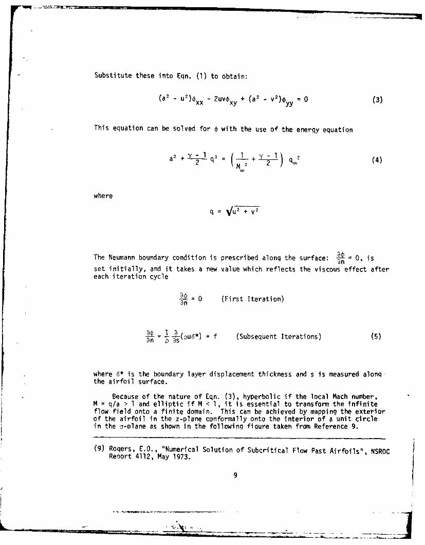
Substitute these into Eqn. (1) to obtain:

(a2 - u2)txx - 2uvxy + (a2 - v2) yy = 0 (3)

This equation can be solved for with the use of the energy equation

a 2 + Y q 2 M(12 + 1 2 1) q.2 (4)

where

q Vu2+ V2

The Neumann boundary condition is prescribed along the surface: 4 = 0, isn

set initially, and it takes a new value which reflects the viscous effect aftereach iteration cycle

0 (First Iteration)n

2 1-(pu6*) = f (Subsequent Iterations) (5)pDn D

where 6" is the boundary layer displacement thickness and s is measured alongthe airfoil surface.

Because of the nature of Eqn. (3), hyperbolic if the local Mach number,M = q/a > 1 and elliptic if M < 1, it is essential to transform the infiniteflow field onto a finite domain. This can be achieved by mapping the exteriorof the airfoil in the z-plane conformally onto the interior of a unit circlein the a-olane as shown in the following figure taken from Reference 9.

(9) Roqers, E.O., "Numerical Solution of Subcritical Flow Past Airfoils", NSROCRer)ort 4112, May 1973.

)Iz)

LEADING TRAILINGEDGE EDGE

GRID IN THE COMPUTATIONAL PLANE GRID IN THE PHYSICAL PLANE

Figure 2. Grid System.

This transformation is particularly useful because an evenly distributedqrid system in the circle plane qives denser finite mesh near the body atthe leadinq and tra'linq edqes in the physical plane where it is needed most.

2.2.2 Mapped Coordinate System

Consider the speed in the z-plane,

q2 u2 + v2 Q1 = l1 B2 + (6)

where

Thus we have

3x ra e' ay ar (7)

*10

The complex potential about a unit circle in a uniform stream is given

by:

w = U(z+ 1) + iEtnz (8)z

Here the velocity potential at infinity becomes unbounded and is of the order

R. Since the present transformation requires the direct inversion of this

external flow, the sinqular behavior at infinity inevitably occurs at the

oriqin of the a-plane.

In order to remove this singularity at the origin, e(l/r), and the dis-continuity at e = 2Tr due to the circulation, a translated potential, G, isintroduced.

cos (8 +. + E(o + x) (9)G= - r

where 2'rE is the circulation, and o is the angle of attack.

Substituting Eqns. (7) and (9) into Eqn. (2) to obtain

(a2 - u2) Gee - 2uvrGr0 + (a2 - v2) r -- (rGr)

- 2uv(G0 - E) + (u2 - v2)G + (u2 + v2)(R B + vB) 0 (10)r r 0 r

where

r(G0 - E) - sin (0 + a) r2Gr - cos (a + a)u= B , v B

The Neumann boundary condition reduces to

Gr = cos (e + a) - at r 1()

11

while the far-field boundary condition becomes

G = Ej+a-tan l - M 2 tan (6+ ] at r = 0 (12)

Here, the circulation constant, E, is determined by the Kutta conditionderived from the upper and lower surface searation pressures and is discussedin a later section.

2.2.3 Inviscid Model of Separated Region

As mentioned earlier, the modelling of the wake is one of the mostimportant elements in the method. One may solve the parabolized Navier Stokesequations for the special class of flow instead of modelling the wake. However,this, in principle, cannot handle the region of large reverse flow. Onthe other hand, solving the full time-dependent Navier Stokes equations isnot practical at this time because of the enormous computing time required.The only logical approach to this oroblem is to simulate the separated flowwith an inviscid wake model. A good wake model, in fact, can represent theactual flow very well as was demonstrated by an earlier study (CLMAX).

In the present model, the separated region is confined by two dividingstreamlines, one from the upper surface separation point and the other fromthe trailinq-edqe point, as shown in Figure 3.

S

Figure 3. Wake Model.

As shown in the figure, along the dividing streamlines the gradient in velocity

potential, 2, is constant, while across the streamlines An is zero.

12

__ I

The wake shape must be updated according to the new separation point.If the separation point remains unchanged, then the solution is consideredto be converqed.

Construction and Transformation of the Wake

Once the separation point, S, on the upper surface is found, the wakeis generated in the following manner (see Fiqure 3). M is the mid-point onthe chord, ST, and the point, J, is fixed at twice the wake width (WD) awayfrom the point, M. The slope of MN is chosen to be .45 times the trailing-edge slooe. Two parabolas can then be constructed through SN and TN, whoseinitial slooes are equal to the body slopes at their respective points.

This wake in the physical plane can now be transformed onto the circleDlane. First, the grid network on the physical plane, which corresponds tothe uniform grid in the circle plane, is generated by using the mappingfunction. With the aid of simple interpolation, the wake in the physicalplane can be readily transformed onto the circle plane. A typical resultingseparated region in the circle plane is shown in Figure 4.

Constant

Fiqure 4. Separated Region in the Computational Plane.

The streamlines which divide the flow into attached and separated flow

reqions represent lines of constant -i . As in the wake model used in Programas

CLMAX, these streamlines represent thin shear layers across which there exists a

a jump in tangential velocity; and, consequently, a jump in velocity potential,

o. Due to this jump, a special treatment in the finite-difference scheme is

necessary along this boundary. In the present scheme, the value of is adjusted

up or down by the amount of jump, AO, where

= ± Asi

13

and As is measured from point S or T, depending on the particular side, tomake the function € continuous across the dividing streamline. With thisaddition and subtraction, the same difference formulae can be used throughoutthe field. The procedure is similar to the so-called "shock-fitting" technique.

The Kutta condition, which is normally applied at the trailing edge, isapplied at points S and T; i.e.,

as as (13)

Special Treatment in Finite-Difference Formulae Along the Dividing Streamline

Constant

M P S s

L 0 R

K

N Q- ___ ___AX _

Figure 5. Finite-Difference Grid.

The main idea of present finite-difference formulae near the dividingstreamline is to make the potential, 1, continuous across this streamline.As previously mentioned, this can be achieved by adding or subtractinq theamount of jump, AO, to or from 0 a, a particular point. The correction isapplied to all points lying on the side opposite the point of finite-dif-ference approximation.

14

As for examples, the derivatives about the point, 0, are shown below.

Wax = N - L)(2 • AX) (14(a))

3/y= P- N - AyN)1(2 * AY) (14(b))

where A1N As

at separation

AsN = arc length along the dividing streamline

326/aX2 = OR - + TL)/Ax 2 (14(c))

= ( p - 2 0 + N - AN))/AY2 (14(d))

2 /;Xqy = k - M + K - ( Q + A4Q))/4(AXAY) (14(e))

2.2.4 Method of Solution

The transFormed Eqn. (10) with boundary conditions, Eqns. (11)and (12), is solved by a finite-difference scheme. Upwind differencing isused when the local flow is supersonic , while central difference formulaeare used at subsonic points. The resulting set of difference equations issolved iteratively. Details of the method are referred to in the originalpaper (Ref. 6) and only the major differences are presented here.

The Kutta condition is imposed by matching the pressures at the uppersurface separation point and the trailing edge; i.e.,

(13)as assep trailing edge

15

1. 7 . . . . . .

The amount of circulation, E, in Eqn. (9) is continuously updated to satisfyEqn. (13). The new estimate of E, determined from the Kutta condition, isthen used for the next iteration. This cycle is repeated until the correctionto E satisfies the convergence criteria.

It was found, during the course of this work, that the method may encountersome difficulty if the solution is sought directly for free stream Mach numbersgreater than 0.35. This occurs because the actual flow is becoming lessstable and will respond rapidly to even small disturbances. When the separationregion is large (greater than 10% chord), the initial inviscid flow field isnot representative of the flow field with separation; consequently, a poorinitial solution can lead to divergent behavior at higher Mach numbers. Properconverqence and stability can be achieved by starting the solution from a lowMach number and raising the Mach number incrementally to the desired value.

After the translated potential, G, is obtained, the tangential velocitycomponent, u, on the surface can be obtained readily throuqh simple dif-ferencing. The pressure coefficient, Cp, alorg the surface is qiven by:

YCp 1[ + - M 2(l - u2) l (15)

2.3 Calculation of Boundary Layer Development

As in the potential flow calculation procedure, new methods for bothlaminar and turbulent boundary layers were adopted. Curle's method forlaminar flow and the Nash-Hicks method for turbulent flow are replaced by theCohen-Reshotko method and Green's method, respectively. However, the sametransition criterion, the Granville procedure, is still intact. The possi-bility of the reattachment as a turbulent boundary layer after laminar boundarylayer separation is also examined on the basis of the Reynolds number basedon the momentum thickness at the point of separation (Ref. 10).

2.3.1 Cohen and Reshotko Method

This integral method was developed for the steady two-dimensionallaminar boundary layer with the assumption that the surface temperature isuniform.

(10) Dvorak, F.A. and Woodward, F.A., "A Viscous/Potential Flow InteractionAnalysis Method for Multi-Element Infinite Swept Wings; Volume I", NASACR-2476, November 1974.

16

First, consider the Stewartson transformation,

_i_=P = -PvaY P 0x PO

a P aeX X e -- t d- X y e_ -_dy

ao Po a0 0

u _ v : - (16)ay aX

where s and a represent the stream function and the speed of sound, respectively.Capital letters denote quantities of the equivalent incompressible problem.With this transformation, the equivalent incompressible problem can be formu-lated. Now, define a parameter,

e 2tr dUen- t (17)

0

where subscript, tr, denotes the transformed coordinate. After somemanipulation, one can obtain

x-- CM -C2 dMe T -4 f M C2-

1 T 4(18n- e dx e e e dx

0

where C1 and C2 are constants.

This can be readily solved for n by simple integration formulae such asthe trapezoidal rule. Then the momentum thickness and the shape factor areobtained from the explicit expressions of n. (See Ref. 7 for details.)

17

-1.~A~

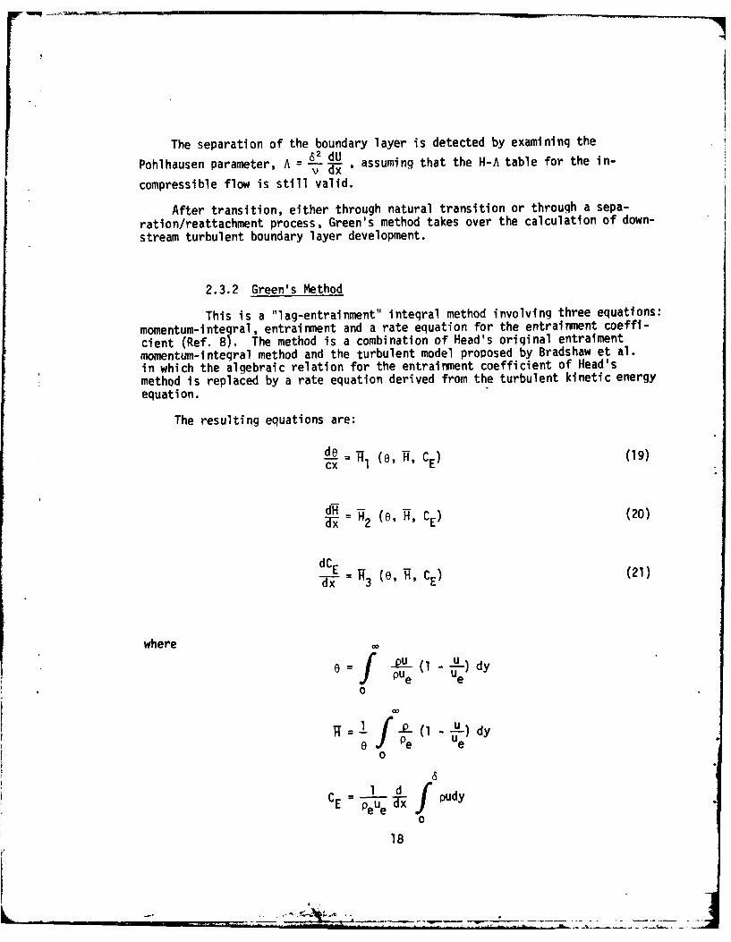
The separation of the boundary layer is detected by examining the=2 dU

Pohlhausen parameter, A =-- Tx , assuming that the H-A table for the in-

compressible flow is still valid.

After transition, either through natural transition or through a sepa-ration/reattachment process, Green's method takes over the calculation of down-

stream turbulent boundary layer development.

2.3.2 Green's Method

This is a "lag-entrainment" integral method involving three equations:

momentum-integral, entrainment and a rate equation for the entrainment coeffi-

cient (Ref. 8). The method is a combination of Head's original entraimentmomentum-integral method and the turbulent model proposed by Bradshaw et al.in which the algebraic relation for the entrainment coefficient of Head'smethod is replaced by a rate equation derived from the turbulent kinetic energyequation.

The resulting equations are:

de = e -ff (19)cx 1 CE)

d-H ( , E (20)

E 2 CE)

dCE (e, , CE) (21)

where 0f / u dl-

PUe dy

0

0

CE 1 d pudy

0

18

This system of ordinary differential equations is solved by the Runge-Kuttamethod. The separation point can be located by monitoring both the frictioncoefficient, Cf9 and the shape factor, H.

19

3.0 RESULTS AND DISCUSSION

The main purpose of this analysis method, TRANMX, is to predict theperformance of a given airfoil for a wide range of angles of attack, and todetermine the maximum lift and its corresponding angle. As will be presentedin this section, TRANMX performs very well for all the cases examined. Thepressure distributions and the C. -a curves are in excellent agreement withthe experimental data.

The method has been tested against four distinctly different airfoils;i.e., GA(W)-l, NACA 0012, Model Al and a Hughes Helicopter Comoany airfoilwith tab. The free stream Mach number varies from .15 for the GAM()-l to.6 for the Al airfoil. For each flow condition, the angle of attack isgradually increased until the airfoil has stalled. Airfoils at angles ofattack beyond the static stall angle have been analysed.

Figure 6(a), (b) and (c) shows the pressure distributions about theairfoil, GA(W)-I, for M. = 0.15 and Re = 6 x 106. It should be noted thatthis is the same test case with which the results of CLMAX were in good agree-ment. The good correlation shown in these figures confirms that these twoanalytical methods are compatible. The computed CZ is a little higher than thedata as shown in Figure 7 due to the slightly higher pressure distributionalong the lower surface. However, this discrepancy of less than 3% is wellwithin the experimental accuracy.

The comoarisons shown in Figures 8 and 9 are for the NACA 0012 symmetricairfoil at M. = 0.5, Re = 3 x l0. Here again the results are quite goodalthough the quoted angles of attack appear to be high. It is interestingto note that the pure inviscid solution for a = 9.86, which is plotted inFigure 8(c), fails to predict the real pressure distribution by a surprisingmargin. A separated region of about 20% of the chord makes the pure poten-tial flow solution meaningless. This indicates that the viscid/inviscidinteration changes the real flow field considerably and the viscous effectscannot be ignored.

The results of two different calculation methods are plotted in Figure 10along with experimental data for a Hughes Helicopter Company airfoil. Thefree stream Mach number is .46 and the Reynolds number is 3.8 million. CLMAXdoes not perform very well, particularly because it is not developed to handlethe highly compressible flow. This also shows the limitation of the usageof linearized equations in compressible flow for this Mach number. TRANMAXperforms well except at the highest angle of attack (Figure 10(c)). In thiscase, the actual flow reaches a local Mach number of 1.5 and the boundarylayer is believed to separate at the foot of the shock. This boundary layer(separation) effectively removes the distinct shock but fails to reattach.This separated flow exhibits quite different characteristics, e.g., varyingpressure along the body, and cannot be treated as well by the present method.The Ci- a curve shown in FiQure 11 is, therefore, rather fortuitous where

20

..... i

. .. . '.. . - - - i -,-i- --- - - - - -- --- -

- GA(W)- MO = 0.15

a = 16.04'

-6 _Re = 6 x 106

c TRANMX

SYMBOLS DATA-4

-2 -- _

0 0C0 -o___

0 0.2 0.4 0.6 0.8 1.0

x/c

(a)

Fiqure 6. Pressure Distribution along GA(W)-I Airfoil.

21

I-..

-10

GA(W)-l M.0 = 0.15

a = 19.06'-8 _____Re = 6 x 106

cp ____ TRANMX

-6 SYMBOLS DATA

0 0.2 0.4 0.6 0.8 1.0X/c

(b)

Fiqure 6. Continued.

22

-101

GA(W)-l M. = 0.15

1; a = 20.05'-8 ____ Re = 6 x 106

p ______ TRANMX

SYMBOLS DATA

-4 -

-2 ____ _____

0 0 0 -

0 0.2 0.4 0.6 0.8 1.0Xlc

(c)

Fiqure 6. Concluded.

23

2.5

c /o o0

01 GA(W)-I

0 Mo" 0.15

Re = 6 x 106

0 TRANMX

1.0SYMBOLS: DATA

0.I I

0 10 20 30

a Deqrees

Fiqure 7. Cz - a Curve for GA(W)-l Airfoil.

24

-4

NACA 0012 Mo = 0. 5C= 3.860

Re = 3 x 106-3 ______

_________ TRANMX

Cp SYMBOLS DATA

-2 ______

0 0.20406 . .

Xlc

(a)

Figure 8. Pressure Distribution along a NACA 0012.

~2

-4q

NACA 0012 Moo = 0. 5a 7.860

Re = 3 x 106

-318____ TRANMX

C SYMBOLS DATA

-2 _____

00

0

0

0 0.2 0.4 0.6 0.8 1.0X/c

(b)

Figure 8. Continued.

26

INACA 0012 MC0= 0. 5ot=9.860

-4 Re =3 x 101-------- FULLY ATTACHED

C0 INVISCID SOLUTION

________ VISCOUS-POTENTIALITERATIVE SOLUTION(AFTER 3RD ITERA- -TI ON)

SYMBOLS DATA

-2 ______

2 0.2 0.4 0. 0.8 _ _ _ _ _

X/c

(c)

Fiqure 8. Concluded.

27

2.0

NACA 0012

M = 0.5

1.5 Re = 3 x 10'

= TRANMX

SYMBOLS = DATA

1.0

00

00.5-

0

0

0 _ _ _ _ _ _ __I_ _I _ _I

0 1.0 20 30

a Degrees

Fiqure 9. C- a Curve for NACA 0012 Airfoil.

28

-4'1

HUGHES HELICOPTERS

Moo~ = 0.46

-3 ____ _______= 6.16010

-2 _______ SYMBOLS DATA

01________

0 0.2 0.4 0.6 0.8 1.0X/c

(a)

Figure 10. Pressure Distribution along a Hughes HelicoptersCompany Airfoil.

29

-5HUGHES HEIOTR

Moo~ = 0.46-4 _______ = 9.390

Re = 3.8 x 101_____ TRANMX

------ CLMAX-3

SYMBOLS DATA

0 0.2_____ 0.4 0.6 o.8 1.

X/c

(b)Figure 10. Continued.

30

-5

HUGHES HELICOPTERS

M. 0.46

=' 11.130

Re =3.3 x 106Cp

-3 TRANMX

---CLMAXP ~SYMBOLS DT

-2 _____

00

0 0.2 0.4 0.6 0.8 1.0X/c

(c)

Fiqure 10. Concluded.

31

2.0

HUGHES HELICOPTERS

M. - 0.461.5 Re = 3.8 x 106

TRANMX

SYMBOLS DATA

1.0

00.5

0

0

0 10 20 30

a Deqrees

Figure 11. Cz - a Curve for a Hughes Helicopters

Company Airfoil.

32

. ... .. . . . . .. -

Another helicopter section, the Al airfoil, results are compa"' inFiqures 12, 13 and 14. The data was collected by Hicks and McCrockey (Ref. 11)in the Ames 2' x 2' Transonic Wind Tunnel with the model airfoil chord of 0.5feet. Among a wide range of test conditions, only the Mach numbers of 0.5and 0.6 are chosen owing to the present interest. The Ct - oL curve shownin Figure 12 can be divided into three regions. The flow in the first region,a < 8', can be characterized by the trailing-edge separation. The lift, Ck,varies nearly linearly with respect to a in this region. The next regionrepresents the flow for angles of attack from 80 to O*CLMAX. The boundarylayer in this region separates at the foot of the shock and thus blunts theshock front. In this region a combination of shock separation and trailing-edqe separation are present. Ck varies gradually in this region until thecatastrophic leading-edge separation brings the lift down sharply in thethird region.

The results are in good agreement with experiment in region I. Thecalculated Ck is much higher than the experimental data in the region II,although the general trend of Ck - a curve is in close agreement with theexperiment. The lower experimental CZ is due to the shock boundary layerseparation which the present method currently cannot predict. The pressuredistributions shown in Figures 13 and 14 correlate very well with theexperimental data. It is interesting to note, in Figure 14, the unsteadybehavior of the pressure in the leading-edge region. This unsteadiness mayindicate the temporary presence of shock boundary layer separation bubble whichwas mentioned earlier.

As we have seen so far in this section, the new calculation method performsvery well for all the cases tested. The minor discrepancies which exist insome of the comoarisons are attributed to the calculation method's ownlimitations rather than inconsistent performance. Misleading high lift, whichis likely to happen when the method does not detect the shock boundary layerseparation, can be easily noted by a careful analysis of the result. Oneobvious clue may be the unrealistically high local speed, say, M > 1.4, sincethe boundary layer through this shock is not likely to remain attached.

Themain difficulty in verifying the calculation method has been the lackof quality transonic flow data. Most of the available data are limited to thecase of no or small separated flow regions. In some cases, e.g., the Al airfoil,the angle-of-attack correction due to tunnel blockage effect is so large (forM = 0.6, Ac z a) that the credibility of the data is in serious doubt. Morereliable high Mach number flow data with a substantial renion of reversedflow are desired for the future improvement of the calculation method.

(11) Hicks, R.M. and McCroskey, W.J., "An Experimental Evaluation of a Heli-copter Rotor Section Designed by Numerical Optimization", NASA TM-78622,March 1980.

33

*w

-4

0AI Mc =0. 496

-3_ __ _ Re =3.52 X 106

cp - _________ ______ TRANMX

-2p SYMBOLS DATA

-1

0 0.2 0.4 0.6 0.8 1.0X/c

Fiqure 12. Pressure Distribution along an Al Airfoilfor M. 0.496; a=8.50.

34

-4

A I o = 0. 596

-3 _ ____ _____Re = 3. 96 x 10 6

___ TRANMX

SYMBOLS DATA

-2 _ _ _ _ _ _ _ _ _ _ _ _ _ _ _ _ _ _ _ _ _

0 0.2 0.4 0.6 0.8 1.0

X/c

Fiqure 13. Pressure Distribution alonq an Al Airfoil

for M.~ 0.596; a =6'.

35

2.0

A 1 co0.5Re =3.5 x 106

1.5 _ TRANMX

SYMBOLS DATA

00

1.0

0.5

0

0 10 20 30

a Deqrees

Fiqure 14. C~ a Curve for Al Airfoil.

36

4.0 CONCLUSIONS

An analysis method for transonic trailing-edge type separated flow has beensuccessfully demonstrated in comparison with experimental data. PredictedCz - a behavior is in good agreement with experiment for several different air-foil types at Mach numbers approaching 0.6. At higher Mach numbers inspectionof the local Mach number distribution usually suggests separation as a result ofstrong shocks. While the program is not currently capable of modelling thisphenomenon, it can be used as a predictive tool to indicate when shock/boundarylayer separation can be expected.

The main advantage of this method over other existing methods is that thepresent scheme with its simple wake model allows computations for massive sepa-ration. It also can be extended to the three-dimensional case where, as pre-viously cited, alternate methods are limited to two-dimensional flow.

37

... . .. . . ' " -- L- - . ' l . ... ... . . .

5.0 REFERENCES

1. Hicks, R., Private Communication, 1977.

2. Diewert, G.S., "Computation of Separated Transonic Turbulent Flows", AIAAPaper No. 75-829, June 1975.

3. Barnwell, R.W., "A Potential Flow/Boundary Layer Method for CalculatingSubsonic and Transonic Airfoil Flow with Trailing-Edge Separation", NASATM-81850, June 1981.

4. Cousteix, J., AFOSR-HTTM-Stanford Conference on: Complex Turbulent Flows,Comparison of Computation and Experiment - Volume I, Stanford University,September 1981.

5. Dvorak, F.A., Maskew, B. and Rao, B.M., "An Investigation of SeparationModels for the Prediction of C ax", Final Technical Report, ContractDAAG29-76-C-0019, Prepared for the U.S. Army Research Office,Research Trianqle Park, N.C., April 1979.

6. Jameson, A., "Numerical Computation of Transonic Flows with Shock Waves",International Union of Theoretical and Applied Mechanics, Springer VerlagNew York, Inc., September 1975, pp.384-414.

7. Burne, G.W. and Manke, J.W., "An Improved Version of the NASA LockheedMultielement Airfoil Analysis Computer Program", NASA CR-15323, March 1978,pp. 69-87.

8. Green, J.E., Weeks, D.J. and Brooman, J.W.F., "Prediction of TurbulentBoundary Lyaers and Wakes in Compressible Flow by a Lag-Entrainment Method",Royal Aircraft Establishment TR-72231, December 1972.

9. Rogers, E.O., "Numerical Solution of Subcritical Flow Past Airfoils", NSRDCReport 4112, May 1973.

10. Dvorak, F.A. and Woodward, F.A., "A Viscous/Potential Flow InteractionAnalysis Method for Multi-Element Infinite Swept Wings; Volume I", NASACR-2476, November 1974.

11. Hicks, R.M. and McCroskey, W.J., "An Experimental Evaluation of a Heli-copter Rotor Section Designed by Numerical Optimization", NASA Th-78622,March 1980.

38

* ....